Modified Adversarial Hierarchical Task Network Planning in Real-Time Strategy Games

College of Information System and Management, National University of Defense Technology, Changsha 410073, China
*
Author to whom correspondence should be addressed.
Appl. Sci. 2017, 7(9), 872; https://doi.org/10.3390/app7090872
Submission received: 31 July 2017
/
Revised: 18 August 2017
/
Accepted: 20 August 2017
/
Published: 25 August 2017
Abstract
:The application of artificial intelligence (AI) to real-time strategy (RTS) games includes considerable challenges due to the very large state spaces and branching factors, limited decision times, and dynamic adversarial environments involved. To address these challenges, hierarchical task network (HTN) planning has been extended to develop a method denoted as adversarial HTN (AHTN), and this method has achieved favorable performance. However, the HTN description employed cannot express complex relationships among tasks and accommodate the impacts of the environment on tasks. Moreover, AHTN cannot address task failures during plan execution. Therefore, this paper proposes a modified AHTN planning algorithm with failed task repair functionality denoted as AHTN-R. The algorithm extends the HTN description by introducing three additional elements: essential task, phase, and exit condition. If any task fails during plan execution, the AHTN-R algorithm identifies and terminates all affected tasks according to the extended HTN description, and applies a novel task repair strategy based on a prioritized listing of alternative plans to maintain the validity of the previous plan. In the planning process, AHTN-R generates the priorities of alternative plans by sorting all nodes of the game search tree according to their primary features. Finally, empirical results are presented based on a µRTS game, and the performance of AHTN-R is compared to that of AHTN and to the performances of other state-of-the-art search algorithms developed for RTS games.
1. Introduction
The application of artificial intelligence (AI) to real-time strategy (RTS) games includes considerable challenges due to the very large state spaces and branching factors, limited decision times, and dynamic adversarial environments involved [1]. RTS games are regarded as a simplification of real-life environments, and could therefore serve as a test bed for investigating activities such as real-time adversarial planning and decision making under uncertainty [2]. Moreover, task planning techniques that have been demonstrated to be effective in RTS games could also be applied in real-world domains [2].
Compared with conventional board games, RTS games have the following primary differences [2]:
- Players can pursue actions simultaneously with the actions of other players, and need not take turns, as in games such as chess. Moreover, player actions can be conducted over very short decision times, allowing for rapid sequences of actions.
- Players can pursue concurrent actions employing multiple controllable units. This is much more complex than conventional board games, where only a single action is performed with each turn.
- Player actions are durative, in that an action requires numerous time steps to be executed. This is also much more complex than conventional board games, where actions must be completed within a single turn.
- The state space and branch factors are typically very large. For example, a typical 128 × 128 map in “StarCraft” generally includes about 400 player controllable units. Considering only the location of each unit, the number of possible states is about 101685, whereas the state space of chess is typically estimated to be around 1050. Of course, even larger values are obtained when including the other factors in the RTS game.
- The environment of an RTS game is dynamic. Unlike in conventional board games such as chess, where the fundamental natures of the board and game pieces never change, the environment of an RTS game may change drastically in response to player decisions, which can invalidate a generated plan.
Because of the differences discussed above, standard game tree search methods, which perform well for board games like alpha–beta search [3], cannot be directly applied in RTS games [4]. However, research has been conducted to modify game tree search methods to address these differences [4]. Chung et al. [5] investigated the applicability of game tree Monte Carlo simulations in RTS games. Balla and Fern [6] applied the upper confidence bound for trees (UCT) algorithm in an RTS game to address the complications associated with durative actions. The UCT algorithm is a variant of Monte Carlo tree search (MCTS) that modifies the strategy of exploring child nodes. The method is believed to adapt automatically to the effective smoothness of the tree. Churchill et al. [7] addressed the complications associated with simultaneous and durative actions by extending the alpha–beta search process. However, the large branching factors caused by independently acting objects still remained a substantial challenge. Methods such as combinatorial multi-armed bandits have attempted to address the challenge of large branching factors [8,9]. Ontañón and Buro [10] addressed very large state space and branch factors by combining the hierarchical task network (HTN) planning approach with game tree search to develop what was denoted as adversarial HTN (AHTN). Here, rather than exploring the entire combination of possible actions, HTN planning could guide the search direction based on domain knowledge. AHTN also extended the HTN planning approach to accommodate simultaneous and durative actions, and applied HTN planning directly into the game search tree to take advantage of standard optimizations such as alpha–beta pruning.
Although AHTN has achieved good performance compared to other search algorithms [10], it still suffers from the following weaknesses.
- The HTN description used by AHTN cannot express complex relationships among tasks and accommodate the impact of the environment on tasks. For example, consider a task involving the forced occupation of a fortified enemy emplacement, denoted as the capture-blockhouse task, which consists of two subtasks. The first subtask involves luring the enemy away from the emplacement (denoted as the luring-enemy subtask), and the second subtask involves attacking the emplacement (denoted as the attacking subtask). Here, the capture-blockhouse task will fail if the attacking subtask fails. However, failure of the luring-enemy subtask would not necessarily lead to an overall failure of the capture-blockhouse task, but would rather tend to increase the cost of completing the parent task because the attacking subtask can still be executed even though the luring-enemy subtask fails. This type of relation cannot be expressed by the HTN description employed in AHTN. Relations related to conditions where subtasks are triggered by the environment or where the execution results of a parent task depend on both the environment and the successful completion of its subtasks also cannot be expressed by the HTN description employed in AHTN.
- AHTN planning cannot effectively address task failures that occur during plan execution. The planning process in AHTN generates a new plan at each frame of the game whenever idle units which are not assigned or execute actions exist. The new plan processing cannot cancel assigned actions of the previous planning. If units have been assigned actions in previous planning, they will keep executing those actions until those actions are failed or completed. In AHTN, each failed task of the previous plan is simply removed at the time of failure without considering its impacts on remaining executing tasks. The remaining tasks will continue executing though these executions may be meaningless. To illustrate this point, we note that, if the failure of a task leads to the failure of its plan directly, the remaining executing tasks of the plan should not be continued execution because they cannot affect the failure of the plan. The remaining executing tasks should therefore be terminated so that the released resources can be employed to repair failed tasks or formulate a new plan. Thus, when one task fails and cannot be repaired, all related tasks in the plan should be terminated, and the AI player should attempt to repair the task to maintain the validity of the original plan.
In this paper, we propose a modified AHTN algorithm with failed task repair functionality, denoted as AHTN-R, to address the two problems discussed above. First, AHTN-R employs an HTN description extended by adding the elements essential task, phase, and exit condition to enhance its capability for expressing complex relationships among tasks and for accommodating the impacts of the environment. Second, AHTN-R employs a monitoring strategy based on the extended HTN description to identify all tasks affected by a failed task. Finally, we develop a novel strategy for repairing failed tasks based on a prioritized list of alternative plans. The priorities of alternative plans are generated by sorting all nodes of the game search tree according to their primary features, and we employ the valid alternative plan with the highest priority to repair the failed task. This method can reduce time consumption by taking advantage of historical information. In each decision cycle, the method attempts to repair failed tasks, followed by a new planning process.
The remainder of this paper is organized as follows. Related work is presented in Section 2. The extended HTN description is presented in Section 3. The AHTN-R planning algorithm is presented in Section 4. Experimental results indicative of the performance of the proposed AHTN-R algorithm are compared with the performances of other algorithms in Section 5. Finally, we conclude the paper and present an indication of future work in Section 6.
2. Related Work
Since the foundation of HTN planning was first proposed by Sacerdoti [11] in 1975, many HTN planners have been proposed, such as the simple hierarchical ordered planner (SHOP) [12] and its successor SHOP2 [13]. Combining HTN planning with search methods guided by human knowledge has been demonstrated to speed up planning dramatically, and this has led some researchers to attempt to apply this approach in typical video games [14]. Menif et al. [15] applied the Simple Hierarchical Planning Engine (SHPE) to Steam Box, which is a type of first person shooter game, using an alternative encoding of planning data. Soemers and Winands [16] investigated the reuse of HTN plans in video games. Numerous examples exist of the successful use of HTN planners in commercial video games [17]. However, to the best of our knowledge, only a few attempts have been made to apply HTN planners to RTS games. Muñoz-Avila and Aha [18] employed an HTN planner to provide human players with explanations for the reasons leading to current states or events according to user queries, and for interrogating the behavior of autonomous players under computer control. Laagland [19] presented the design, implementation, and evaluation of an HTN planner in an open source RTS game denoted as Spring. The planning of the RTS game was divided into three levels with the HTN planner being employed in the highest strategic level. Laagland [20] further summarized the advantages and disadvantages of HTN planning in RTS games. Naveed et al. [21] employed HTN planners to reduce the size of the pathfinding search space in RTS games, and tested their algorithm in games developed using ORTS in 2010. Most recently in 2015, Ontañón and Buro [10] developed the AHTN algorithm and applied it to RTS games.
Of the above studies, we note that no research other than that of Ontañón and Buro [10] has considered the adversarial feature of RTS games. Moreover, no research has adequately addressed task failures that occur during plan execution in RTS games. However, studies focused in other fields have addressed task repair based on HTN. Garzón et al. [22] proposed a task repair strategy based on HTN planning to adapt to failures during the execution of treatment plans generated by therapy planning systems. The strategy employed three methods for effecting task repair: application of the knowledge base, search of alternative decompositions, and operator notification. Gateau et al. [23] employed HTN to repair failed tasks to as localized an extent as possible in a high-level distributed architecture for multi-robot cooperation. The core concept of the strategy was to re-plan only a sub-tree of the plan based on a hierarchical structure. Ayan et al. [24] designed an extension of SHOP to repair failed tasks by introducing a task-dependency graph. Here, only that portion of the original plan related to the failed task was subjected to re-planning. The task-dependency graph was employed to record causal links in the task network, and was then applied to eliminate the effects of re-planning on the other portions of the original plan, and to reduce the cost of re-planning. The approach applied re-planning only to the affected parts of the task network using HTN. However, many of these approaches failed to take advantage of the information generated in the previous planning process to reduce the cost of task repair.
3. Extended HTN Description
This section presents an extended HTN description to express complex relationships among tasks and accommodate the impacts of the environment on tasks. We first analyze the requirements for extending the HTN description, and then present a formal definition of the extended HTN description.
3.1. Requirements Analysis
The HTN planning approach generates plans by decomposing tasks recursively into smaller subtasks [25]. HTN planning includes two types of tasks: primitive tasks and compound tasks. Primitive tasks correspond to actions that can be executed by an agent directly in the game environment, such as a specific movement. Compound tasks represent goals that must be achieved by a high-order plan and decomposed into a task network.
3.1.1. Essential Task Attribute
In AHTN planning, the result of a compound task depends on the results and logical relationships of its subtasks. Its task decomposition tree is an and-or-tree with logical relationships between subtasks that are either AND or OR. The AND relationship indicates that the failure of any subtask will lead to a failure of its parent task. The OR relationship indicates that the success of any subtask will lead to the success of its parent task. However, some domain knowledge regarding the completion of a task cannot be represented by an and-or-tree. Returning to the capture-blockhouse task example discussed in the introduction, we note that the success of the luring-enemy subtask may decrease the cost of completing the parent task, but its failure would not lead to the failure of its parent task. However, the success and failure of the capture-blockhouse task is completely dependent on the success and failure of the attacking subtask. These more complex logical relationships cannot be represented by the formation of an and-or-tree.
To represent task decomposition reflecting more complex logical relationships, we introduce an attribute denoted as essential task, whose value is either true or false, and this attribute is applied to all tasks of the HTN. Here, the failure of any essential task will automatically lead to the failure of its parent task without consideration for the results of any other subtasks. For two subtasks and , their logical relationships are represented as follows:
- if the essential task attributes of both are true, the relationship between and is AND;
- if the essential task attributes of both are false, the relationship between and is OR;
- if the essential task attribute of only one is true, the relationship is neither AND nor OR.
3.1.2. Phase and Exit Condition Attributes
The result of a compound task not only depends on the relationships and results of its subtasks, but sometimes also depends on the environment, which can change dynamically. These impacts from the environment can be of the following two types.
- The environment can control the start of tasks once previous tasks have been completed. For example, the task associated with the sudden concealed attack on an enemy, denoted as the ambushing-enemy task, consists of two subtasks: the first is associated with movement to the staging area of the ambuscade, denoted as move-to-ambushing-area, and the actual activity of attacking, denoted as attack-enemy. It is obvious that the attack-enemy subtask could not be executed immediately upon completing the move-to-ambushing-area subtask because the attack-enemy task cannot be executed until the enemy resides in the ambuscade area.
- The environment could necessitate the failure of a task. For the ambushing-enemy task example, the move-to-ambushing-area subtask must be completed before the enemy has passed the ambuscade staging area; otherwise, the ambushing-enemy task would fail.
While the AHTN algorithm can accommodate the first type of impact using the preconditions of tasks, the second type of environmental impact cannot be addressed. In this paper, we propose the exit condition attribute to address these two types of environmental impacts. The exit condition attribute can be divided into sufficient exit condition and necessary exit condition attributes. If a task has some necessary exit conditions, its subsequent task cannot be executed until all necessary exit conditions are satisfied. If a task has some sufficient exit conditions, its parent task will fail when any sufficient exit condition is satisfied but the task is not completed. The exit condition attribute is written using a Lisp-like syntax like the precondition defined in [13].
The phase attribute is proposed to describe the relationships between subtasks that reflect the fact that the execution of a compound task can be divided into several sequential steps, and each step may include parallel subtasks. Because tasks in the same phase are often affected by the same exit conditions, we add the set of exit conditions to the phase rather than adding them to each task.
For an example, we return to the ambushing-enemy task, where we have modified the task to consist of three subtasks: move-to-ambushing-area, surveil-enemy, and attack-enemy. The modification includes the subtask surveil-enemy reflecting the requirement to first determine that the enemy resides in the ambuscade area prior to attacking. The first two subtasks are executed in parallel using different units and the attack-enemy can be executed only when the first two subtasks are completed. We divide the execution of ambushing-enemy into two phases. The subtasks move-to-ambushing-area and surveil-enemy are included in the first phase, which is denoted as the preparatory-phase. The attack-enemy subtask is included in the second phase, denoted as the attack-phase. The preparatory-phase has both sufficient and necessary exit conditions, where the ambushing-enemy task will fail if the subtasks of the preparatory-phase have not been completed by the point at which the enemy has passed the ambushing-area (i.e., the sufficient exit condition is satisfied), and the attack-enemy task will not be initiated if the subtasks of the preparatory-phase have been completed while the enemy has not passed the ambushing-area (i.e., the necessary exit condition is not satisfied). The data structures employed in the example are shown in Figure 1, where the units denoted as ?unitid1 and ?unitid2 will ambush the enemy denoted as ?enemy at the ambushing-area denoted as ?place. In the preparatory-phase, ?unitid1 is allocated to move to ?place and ?unitid2 surveils ?enemy. If the preparatory-phase is completed, ?unitid1 will attack ?enemy. Additional definitions are provided in the following subsections.
Including the phase attribute during the decomposition of a compound task is the main difference between the AHTN used in this paper and that in [10]. The definition of the phase attribute is as follows.
Definition 1
(phase). The phase attribute is defined as a tuple: , where the following definitions apply.
- is the name of the phase.
- consists of the name of the method to which the phase belongs and a list of parameters for the phase.
- is the set of sufficient exit conditions. Each element is a logic expression of literals which consist of the name and a list of parameters.
- is the set of necessary exit conditions. Each element is a logic expression of literals which consist of the name and a list of parameters. Here, subsequent phases can be executed only when all necessary exit conditions are satisfied.
- is the set of subtasks that should be completed to accomplish a compound task. The subtasks can be either compound tasks or primitive tasks. Each element in consists of the subtask’s name and a list of parameters.
Because a phase is executed sequentially, any failure of a phase will lead to the failure of the method associated with that phase. The result of a phase depends on two factors: tasks and sufficient exit conditions. Accordingly, the following four conditions lead to the failure of a phase:
- Any essential task of the phase has failed.
- Any sufficient exit condition is satisfied, with one or more essential tasks still executing.
- Any sufficient exit condition is satisfied, and no subtasks have been completed.
- All subtasks have failed.
For 1, the failure of any essential task means that the parent task has failed, and its phase is also considered as failed. For 2, uncompleted essential tasks cannot continue executing when a sufficient exit condition is satisfied, and the parent task also fails. In addition, according to 3, the phase will fail when no subtasks are completed and a sufficient exit condition is satisfied. Finally, a task obviously fails if all its subtasks have failed.
3.2. Definition of the Extended HTN Description
An HTN problem can be defined as a tuple: , where the following definitions apply:
- is the set of current world states, and consists of all information that is relevant to the planning process.
- is the set of task decomposition methods. Each method can be applied to decompose a task into a set of subtasks.
- is the set of operators. Each operator is an execution of a primitive task.
- is the current task network. It is a tree whose nodes are tasks, methods, or phases.
- is the state transform function. Given , defines the transition of the state when an primitive task is executed by an agent. If , the operator is not applicable in .
The definition of a method in the proposed extended description is similar to the definition employed in previous HTN descriptions. However, our method uses the list of phases rather than sets of subtasks, and adds the attribute denoted as essential.
Definition 2
(method). A method is defined as a tuple: , where the following definitions apply.
- is the name of the method.
- is the name of the task to which the method is applied.
- is the logical preconditions for the method, which should be satisfied when the method is applied.
- is the list of phases. The sequence of the elements in is the execution sequence.
- is a Boolean value, and is true to indicate that a task to which the method is applied is an essential task.
The definition of an operator is also similar with that in previous HTN descriptions except for adding the essential attribute.
Definition 3
(operator). The operator is defined as a tuple: , where the following definitions apply.
- is the primitive task that can be applied by this operator.
- is the precondition that must be satisfied before task execution.
- are the delete effects.
- are the add effects.
- is a Boolean value, and is true to indicate that the task to which the operator is applied is an essential task.
4. AHTN-R Planning Algorithm
The overall framework of the AHTN-R algorithm is provided firstly, and the functions of its different components are explained. Then, the monitoring strategy employing the extended HTN description is proposed to address the issue of failed tasks. Finally, we discuss the proposed failed task repair strategy.
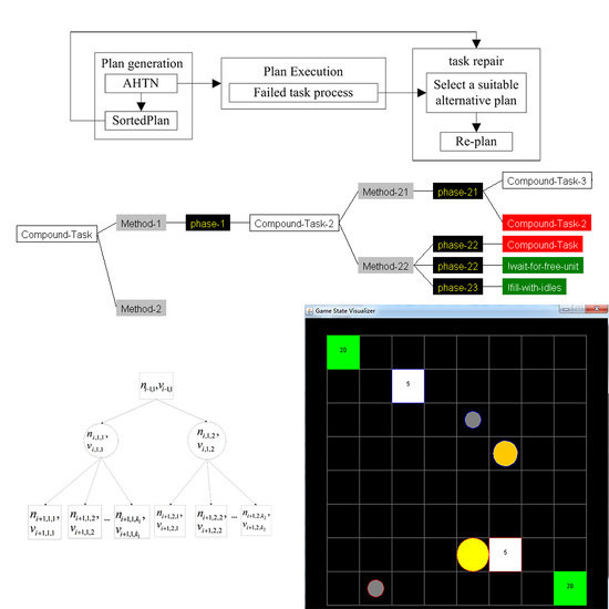
4.1. ATHNR Framework
The overall framework of the AHTN-R algorithm is illustrated in Figure 2. The process flow consists of three main components: plan generation, plan execution, and task repair. The plan generation component provides the best plan to the plan execution component, and provides a prioritized list of alternative plans to the task repair component. The plan execution component processes the failed tasks responsible for plan failure and sends the task needing repair to the task repair component. The task repair component attempts to repair failed tasks at the beginning of each decision cycle.
At each decision cycle, when there are idle units, the plan generation component will search the best plan using the AHTN algorithm with the extended HTN description. This paper modified the part of the AHTN algorithm obtaining the next action. In AHTN, the subtasks can be obtained if a method is applied. However, with the introduction of phase in AHTN-R, the phases will be obtained rather than the subtasks if a method is applied. The AHTN-R algorithm accesses the generated phases to obtain the next primitive task. Algorithm 1 shows the method employed to obtain the next executable action based on the HTN plan N and execution pointer t, which keeps track of which parts of N have already been executed. The result of Algorithm 1 is a primitive task or an empty set, indicating an absence of an available primitive task. Lines 1–4 show that, if no tasks have yet been executed, the algorithm returns the first primitive task in N. Lines 7–19 show that, if all tasks in the same phase with t have been executed, the algorithm searches the first primitive task from the next phase. If no primitive tasks are found in the next task, an empty set is returned. Lines 20–31 show that the algorithm searches for a primitive task from the remaining tasks in the same phase that have not been executed.
| Algorithm 1 Returns |
| 1. If then |
| 2. Get the root of N, denoted as the |
| 3. Return |
| 4. End If |
| 5. Acquire the phase p to which t belongs |
| 6. Get all tasks denoted as of |
| 7. If all tasks in have been executed then |
| 8. Get the next phase of |
| 9. If then |
| 10. Return |
| 11. End If |
| 12. Get all tasks denoted as of |
| 13. For all do |
| 14. If then |
| 15. Return |
| 16. End If |
| 17. End For |
| 18. Return |
| 19. End If |
| 20. For all that have not been executed do |
| 21. If is a primitive task then |
| 22. Return |
| 23. End If |
| 24. Get the first phase of the method applied to |
| 25. Get all tasks denoted as of |
| 26. For all do |
| 27. If then |
| 28. Return |
| 29. End If |
| 30. End For |
| 31. End For |
| 32. Return |
Once the best plan is generated, the AHTN-R will obtain the prioritized listing of alternative plans generated by AHTN through sorting the nodes of the game search tree. The method of sorting plans is discussed in Section 4.3. During plan execution, the task may fail because of the dynamics of the RTS game environment. Once a task fails, AHTN-R will process the failed task according to the monitoring strategy discussed in Section 4.2, which seeks to identify and terminate the smallest possible set of tasks affected by the failed task. In this way, the effects of a failed task can be limited to the smallest scope possible.
At the beginning of each decision cycle, AHTN-R first attempts to repair the failed task by selecting a suitable plan from the list of alternative plans according to their priorities. AHTN-R will then execute the tasks of the alternative plan corresponding to the tasks affected by the failed task. If AHTN-R is unable to find a suitable alternative plan, it will generate an altogether new plan for the failed task by AHTN. This process is discussed at the end of Section 4.3.
4.2. Failed Task Monitoring Strategy Using the Extended HTN Description
Once a task fails, an AI player must identify and terminate all tasks affected by the failed task. To accomplish this, the sources of the plan failure are analyzed first. Plan failure can be attributed to two sources: the failure of actions and the state of the sufficient exit conditions attribute. An action will fail when its unit is destroyed or when available resources cannot be obtained to fulfill the action. A plan may also fail if the sufficient exit condition is satisfied, as discussed in Section 3.1.2. Task failure triggers the monitoring strategy. Algorithm 2 shows the main process of the strategy employed to monitor failed tasks.
The input of Algorithm 2 is the failed task t, and the result of Algorithm 2 is a list denoted as RepairTaskList, which contains the tasks requiring repair. Lines 1–4 show the different strategies for addressing essential and unessential tasks. Lines 5–15 show how failed compound tasks are addressed. Lines 7–13 show that, if a failed compound task has available methods, it will be saved and repaired in the next decision cycle. Only when a task has no available methods will it be considered as the failed task. In this way, the number of affected tasks will be as small as possible, which will reduce the extent of repair required. Line 15 shows the strategy for addressing primitive and compound tasks without available methods.
| Algorithm 2 Return TaskFailed(t) |
| 1. If then |
| 2. SubTaskFailed(t) |
| 3. Return |
| 4. End If |
| 5. If t is a compound task then |
| 6. Acquire all methods m of t |
| 7. For each method |
| 8. Get the precondition set of |
| 9. If all is satisfied then |
| 10. Add t into RepairTaskList |
| 11. Return |
| 12. End if |
| 13. End For |
| 14. End if |
| 15. SubTaskFailed(t) |
According to the extended HTN description, each task, except the root node task, belongs to a single phase, and whether the phase corresponding to a failed task has also failed must be determined. Algorithm 3 shows the strategy for addressing the corresponding phase according to the HTN description presented in Section 3.2. The input of Algorithm 3 is a task t. Line 2 shows that, if the failed task is the root node task, it need not be repaired. If the phase is failed, Algorithm 4 and Algorithm 5 are called to terminate the affected tasks and process compound tasks. The failed phase serves as the input of Algorithms 4 and 5. Algorithm 4 shows the strategy for processing the failed phase. If the task belonging to the failed phase is a compound task, its subtasks will be processed, and, if it is a primitive task, it will be terminated directly. Algorithm 5 shows the strategy for processing the method to which the failed phase belongs. Lines 2–6 show that all unfinished phases of the method are failed because they are sequential.
| Algorithm 3 SubTaskFailed(t) |
| 1. Acquire the phase corresponding to t |
| 2. If then return |
| 3. End If |
| 4. If one of the sufficient conditions of is met then |
| 5. If any essential tasks of are failed then |
| 6. PhaseFailed(); |
| 7. MethodFailed(); |
| 8. Else If has no essential task |
| 9. (all tasks of were executed or did not start) |
| 10. PhaseFailed(); |
| 11. MethodFailed(); |
| 12. End If |
| 13. End If |
| 14. Else If any essential tasks of fail |
| 15. ( has no essential task all tasks of fail) |
| 16. PhaseFailed(); |
| 17. MethodFailed(); |
| 18. End If |
| 19. End If |
If any sufficient exit condition is satisfied, the AI player will determine whether the phase to which the sufficient exit condition belongs has failed. The processing involved is similar to that given by Algorithm 3 except that its input parameter is a sufficient exit condition rather than a failed task.
| Algorithm 4 PhaseFailed() |
| 1. Get all tasks denoted as of |
| 2. For all tasks |
| 3. If then |
| 4. continue; |
| 5. End If |
| 6. If t is a compound task then |
| 7. Get the method m applied to t |
| 8. Get all phases within of m |
| 9. For all phases |
| 10. PhaseFailed(q) |
| 11. End For |
| 12. Else |
| 13. Cancel(t) |
| 14. End If |
| 15. End For |
| Algorithm 5 MethodFailed (p) |
| 1. Get the method m to which p belongs |
| 2. For all phases of m |
| 3. If then |
| 4. PhaseFailed(q) |
| 5. End If |
| 6. End For |
| 7. Get task t to which m is applied |
| 8. TaskFailed(t) |
4.3. Task Repair Strategy Based on the Priorities of the Alternative Plans
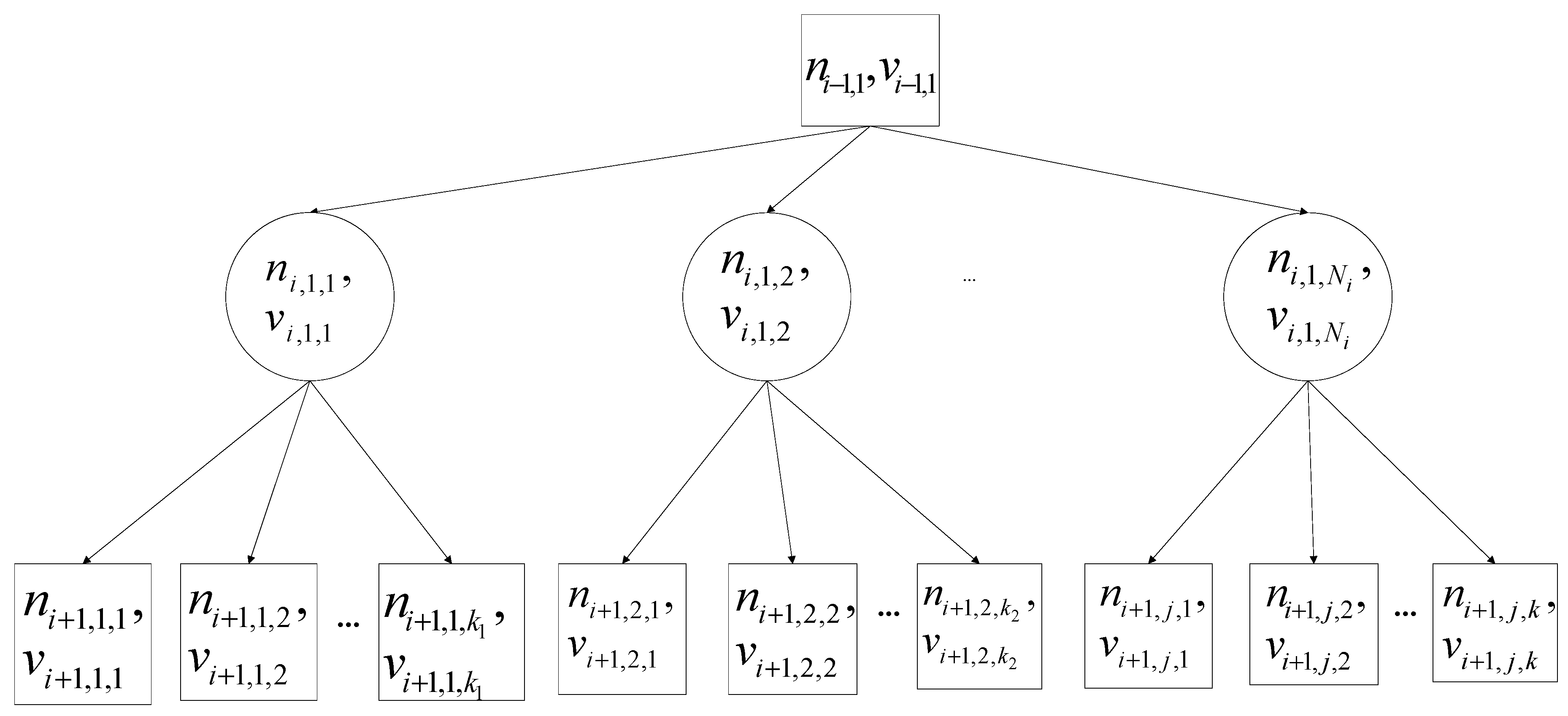
At each decision cycle, the AI player attempts to find an alternative plan for each task in RepairTaskList based on the information included in previous planning. Here, if all plans generated during previous planning could be saved, the AI player could generate a repair plan by searching the previously generated plans rather than constructing a new plan for the failed task directly. This will reduce the time consumed by the task repair process. To accomplish this, the AI player generates some alternative plans with different evaluations during each task planning period. These evaluations establish the priorities of the alternative plans. The evaluations are based on two primary features of the alternative plans: their task decompositions and task parameters. For example, a task T can be decomposed into tasks sub-T1 and sub-T2, or sub-T3 and sub-T4. Each constructs a plan. The planner will compute the evaluations for executing T according to the two plans, respectively. If one fails during execution, the planner will employ the other to repair T. Better repair performance will be obtained by conducting a search according to the priorities of the alternative plans, beginning with the alternative plan with the highest priority. However, aside from the best plan, the plans generated by the AI player are usually out of order. Therefore, the generated alternative plans must be recorded in descending order according to their evaluations. At the same time, because the alternative plans form the leaves of the game search tree in the AHTN algorithm, the reordering of plans is equivalent to the reordering of leaf nodes. To accomplish the above processing, we propose Theorem 1 and prove the validity of the ordering thereby obtained as follows.
Theorem 1.
Given an m-level min–max search tree, the ith level has Ni nodes, where each node is represented by ni,j (i ≤ m, j ≤ Ni). The sub-nodes of ni,j are ordered according to the following two conditions.
- 1.
- if ni,j (i.e., the parent node) is a max node, its subnodes (or child nodes) are ordered decreasingly from left to right according to their evaluations;
- 2.
- if ni,j is a min node, its subnodes are ordered increasingly from left to right according to their evaluations.
The above ordering of all nodes of the min-max search tree represent the proposed prioritizing of plans, where the plan of the left node will better than the plan of the right node.
Proof.
We employ the min–max search tree illustrated in Figure 3 as an example, where max nodes and min nodes are represented by rectangular and circular boxes, respectively. Here, are subnodes of and are subnodes of . We assume that is a max node. The evaluations are denoted by the variable v. For example, the evaluation of is represented by , where the subnode evaluations of are ordered decreasingly from left to right as . In addition, we assume that is a min node, so that its subnode evaluations are ordered increasingly from left to right as . With being a max node, we obtain the relationships and . When the best plan node is removed, the value of will become , and the values of the other subnodes of will not change. Therefore, the value of will become , and the best plan node is . If we continue the process of removing the best plan node, the best plan node will become . When all subnodes of have been removed, the best plan node will become the first subnode of . For , the order of best plans is the same as the order of . If is a min node, the conclusion will not change.
Algorithm 6 shows the main process of sorting plans according to their evaluations. The input of Algorithm 6 is a node of the game search tree. The sorting process begins with the root node of the game search tree. The algorithm sorts all nodes of the game search tree from the top down. Lines 2–4 check whether the input node is a leaf node. Lines 5–9 sort all subnodes of the input node according to Theorem 1. Lines 10–12 process each subnode of the input node iteratively.
| Algorithm 6 SortedPlan(root) |
| 1. Get the list of all subnodes of root |
| 2. If then |
| 3. Return |
| 4. End If |
| 5. If root is a max node then |
| 6. Sort decreasingly according to subnode evaluations |
| 7. Else |
| 8. Sort increasingly according to subnode evaluations |
| 9. End If |
| 10. For each |
| 11. SortedPlan() |
| 12. End For |
After conducting the above process, the generated alternative plans are provided to the AI player for repairing failed tasks. However, prior to conducting task repair, we must determine the location of the failed task within the alternative plan, and execute that part of the alternative plan in place of the failed task. Because the same task can be used as a subtask of different compound tasks, it is necessary to compare both the name and decomposition path to confirm the location of the failed task within the alternative plans. When the failed task has been found in an alternative plan, its leaf nodes will be considered as the new actions to be executed.
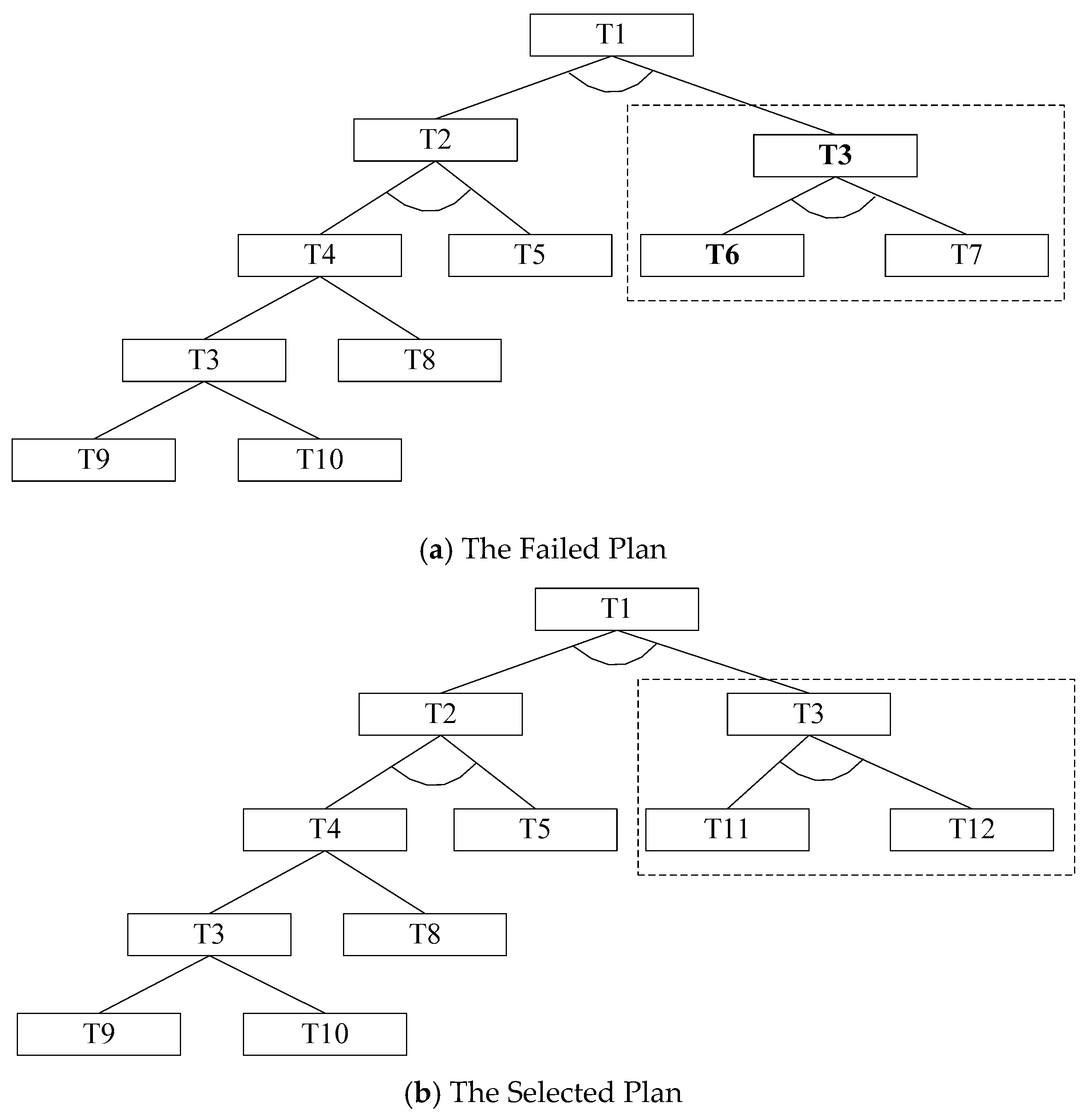
An example is given in Figure 4, where Figure 4a shows a plan that has failed owing to the failure of essential task T6 (given in bold font). The failure of T6 requires the repair of T3, which is a subtask of T1, and does not affect T2. AHTN will only remove T6 and continue executing remaining tasks even though the plan has failed. However, AHTN-R can select an alternative plan, which applies another method to T3. AHTN-R executes new subtasks T11 and T12 in place of subtasks T6 and T7, which is marked by the dashed-line box in Figure 3b.
5. Experimental
5.1. Experimental Environment and Settings
We compared the performance of the proposed AHTN-R algorithm with other algorithms [26] using free µRTS software [27], which has been used in the past to evaluate various algorithms applied in RTS games [4,9,10]. A screenshot of the µRTS game environment is shown in Figure 5. Here, the units of two players (denoted by the blue and red outlines) compete to destroy the units of their opponent. Each player has the same types of units. The small gray circles are workers that can attack enemies, build bases, and harvest and transport resources. The green squares are the limited resources that can be harvested. The orange circles are light attackers, and the yellow circles are heavy attackers. The heavy and light attackers both have larger hit and health points than the workers, making them more effective and resilient attackers, but they cannot harvest or transport resources. The white squares are bases that can produce new units. The µRTS game environment provides six types of actions for units: move into any empty space in the four cardinal directions, attack any enemy in range, harvest minerals from resource units, return minerals to bases, produce new units in any empty spaces in one of the four cardinal directions (for workers and bases), and remain idle, where the unit takes no action. Although µRTS provides simplified RTS games, the games are sufficiently complex, and exhibit the standard challenges of RTS games, such as concurrent player activity, durative and simultaneous actions, real-time limitation, and large branching factors. The original µRTS is deterministic and fully observable.
The comparison evaluation considered the standard AHTN algorithm in addition to the following collection of search algorithms.
- Randombiased: An AI player employing a random biased strategy that executes actions randomly.
- LightRush: A hard-coded strategy. This AI player produces light attackers, and commands them to attack the enemy immediately.
- HeavyRush: A hard-coded strategy. This AI player produces heavy attackers, and commands them to attack the enemy immediately.
- UCT: We employ an implementation with the extension for accommodating simultaneous and durative actions [10].
The following parameters were employed in the testing.
- CPU time: The limited amount of CPU time allowed for an AI player per game frame. In our experiments, we employ different CPU time settings from 20 to 200 ms to test the performances of the algorithms.
- Playout policy: The Randombiased playout policy is employed for the AHTN-R, AHTN, and UCT algorithms in our experiments [10].
- Playout time: The maximum running time of a playout. The playout time is 100 cycles.
- Pathfinding algorithm: In our experiments, the AI player employs the A* pathfinding algorithm to obtain the path from a current location to a destination location.
- Maximum game time: The maximum game time is limited to 3000 cycles. This means that, if both players have living units at the 3000th cycle, the game is declared a tie.
- Maps: The three maps used in our experiments are M1 (8 × 8 tiles), M2 (12 × 12 tiles), and M3 (16 × 16 tiles).
To evaluate each algorithm, we conduct a round-robin tournament, in which each algorithm plays 50 games (with various starting positions) against all other algorithms in each of 3 different maps (8 × 8 × 50 × 3 = 9600 games in total). The method used to compute the score of each algorithm is as follows: the winner of each game was awarded 1 point, and both algorithms were awarded 0.5 points in the event of a tie. Each of the two AI players in all competitions began with a single base, an equivalent resource value, and a single worker.
To compare the performance of our AHTN-R algorithm with the performance of the standard AHTN algorithm, we crafted two different HTNs for the µRTS domain, which are defined as follows.
- Low Level: contains 12 operators (primitive tasks) and 9 methods for 3 types of tasks.
- Flexible: contains the 12 operators of the Low Level, but provides 49 methods and 9 types of tasks. This functionality allows methods to employ parallel execution tasks.
The employment of the Low Level and Flexible HTNs in the AHTN and AHTN-R algorithms are denoted subsequently as, e.g., AHTN-R-LL and AHTN-R-F, respectively. Naturally, the HTNs used by the AHTN-R algorithm employ the extended HTN description. All tasks except for wait-for-free-unit and wait in HTNs are defined as essential tasks. Some of the phases include exit conditions to reflect the influence of the environment. Figure 6 shows an example task from the Low Level HTN. The task named destroy-player-internal can be decomposed into two subtasks unit-order and destroy-player-internal by applying the method dpi-nextunit when the precondition is satisfied. Because the two subtasks are parallel, they belong to the same phase, denoted as dpi-nextunit-phase. Because one subtask is the same as its parent task, we will focus on subtask unit-order. If the preconditions of its method uo-attack are satisfied, this task will be decomposed into the subtasks move-into-attack-range and attack. The subtasks belong to the different phases: preparatory-phase and attack-phase because they must be performed sequentially, and both are essential tasks. We note that attack-phase-1 has a necessary exit condition, indicating that subtask attack in the subsequent phase cannot be executed until the necessary exit condition is satisfied. Because the essential attributes are all true in Figure 6, the failure of move-into-attack-range or attack will lead to repair unit-order. If unit-order cannot be repaired, the planner will terminate all tasks in dpi-nextunit-phase and try to repair its parent task.
5.2. Experimental Results and Analysis
In this section, we compare the performance of AHTN-R with the other algorithms in terms of the average score, average decision time, and average failed task repair rate for the three maps. Each algorithm will play 700 games in total against the other algorithms as player 1 or player 2 and 50 games against itself. Because data are collected from both players, the average score of each algorithm shown in Figure 7, Figure 8 and Figure 9 is obtained effectively over 800 games. The average decision time for each algorithm shown in Figure 10, Figure 11 and Figure 12 is effectively the average value of 100 games against eight types of AI players, respectively. The average failed task repair rate of AHTN-R is also obtained in the same way.
5.2.1. Average Score under Different CPU Time Settings for the Three Maps
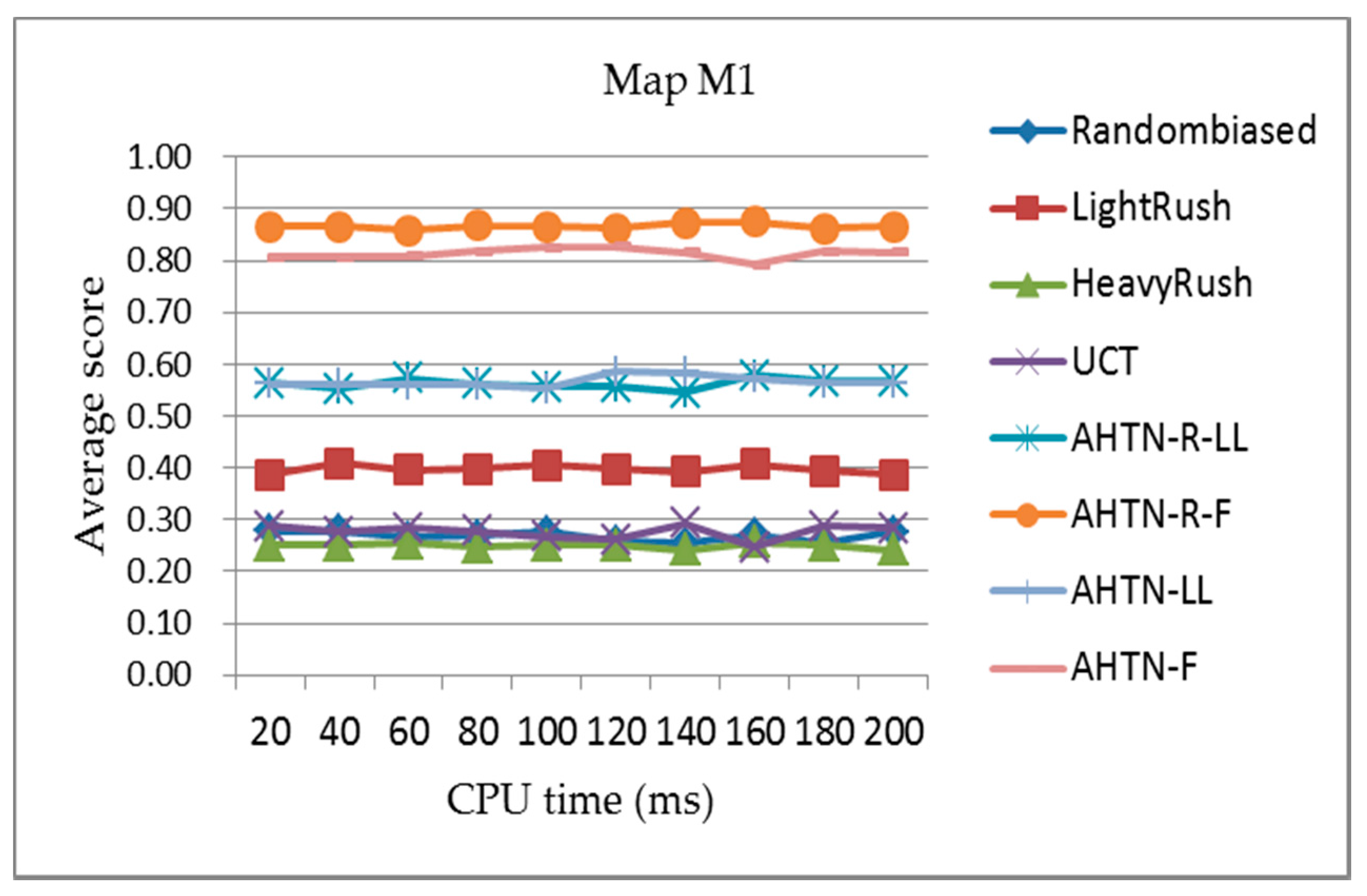
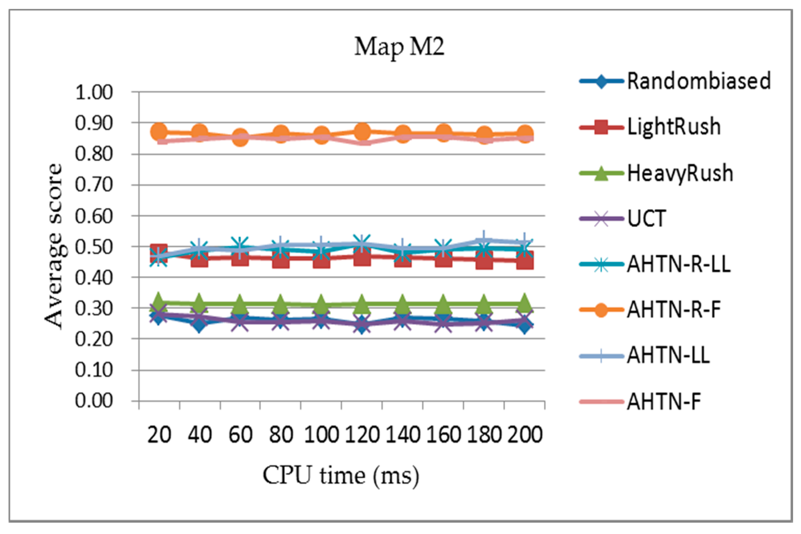
Figure 7, Figure 8 and Figure 9 present the comparisons of the average scores obtained for each algorithm during the round-robin competition with respect to the CPU time from 20 to 200 ms for the three maps. According to the results, we can see that the AHTN-R-F player outperforms all other AI players on all three maps under different CPU times. In addition, the performances of AHTN-R-F vary little with the increasing scale of the maps, and are very stable with respect to CPU time. AHTN-R-F outperforms AHTN-F because of the greater flexibility of AHTN-R than AHTN in a dynamic environment. Here, AHTN does not consider the effects of failed tasks, while AHTN-R identifies and terminates all tasks affected by the failed task, which allows AHTN-R to make more efficient use of available units and resources. AHTN-R also attempts to repair failed tasks in as local an extent as possible in an effort to maintain the validity of the previous plan. AHTN-R-F performs best because it uses an improved HTN domain knowledge for guiding the game tree search, which yields a good plan in a relatively short time.
With respect to the other algorithms, we note that AHTN-R-LL and AHTN-LL have similar performances on the smallest map. However, the performance of both AHTN-R-LL and AHTN-LL deteriorate as the map size increases, and AHTN-R-LL generally performs worse than AHTN-LL on the largest map. The performances of both players deteriorate because more units are produced on the larger maps and the domain knowledge obtained by AHTN-R-LL and AHTN-LL is too simple to adapt to such a complex game. For AHTN-R, the poor domain knowledge means that the previous plan may not be suitable for the current condition, and it would be better to construct a new plan. The relative performances of the scripted methods HeavyRush and LightRush are also observed to improve with increasing map size, which is owing to the underperformance of AHTN-R-LL and AHTN-LL on larger maps.
With respect to CPU time, the performances of all AI players change very little for all three maps. This is because all AI players require little time to make decisions. However, if the CPU time is very small, the performance will deteriorate. Because the performances of all AI players were similar under different CPU time settings, we employed a single CPU time setting of 100 ms in subsequent experiments.
5.2.2. Average Decision Time for the Three Maps
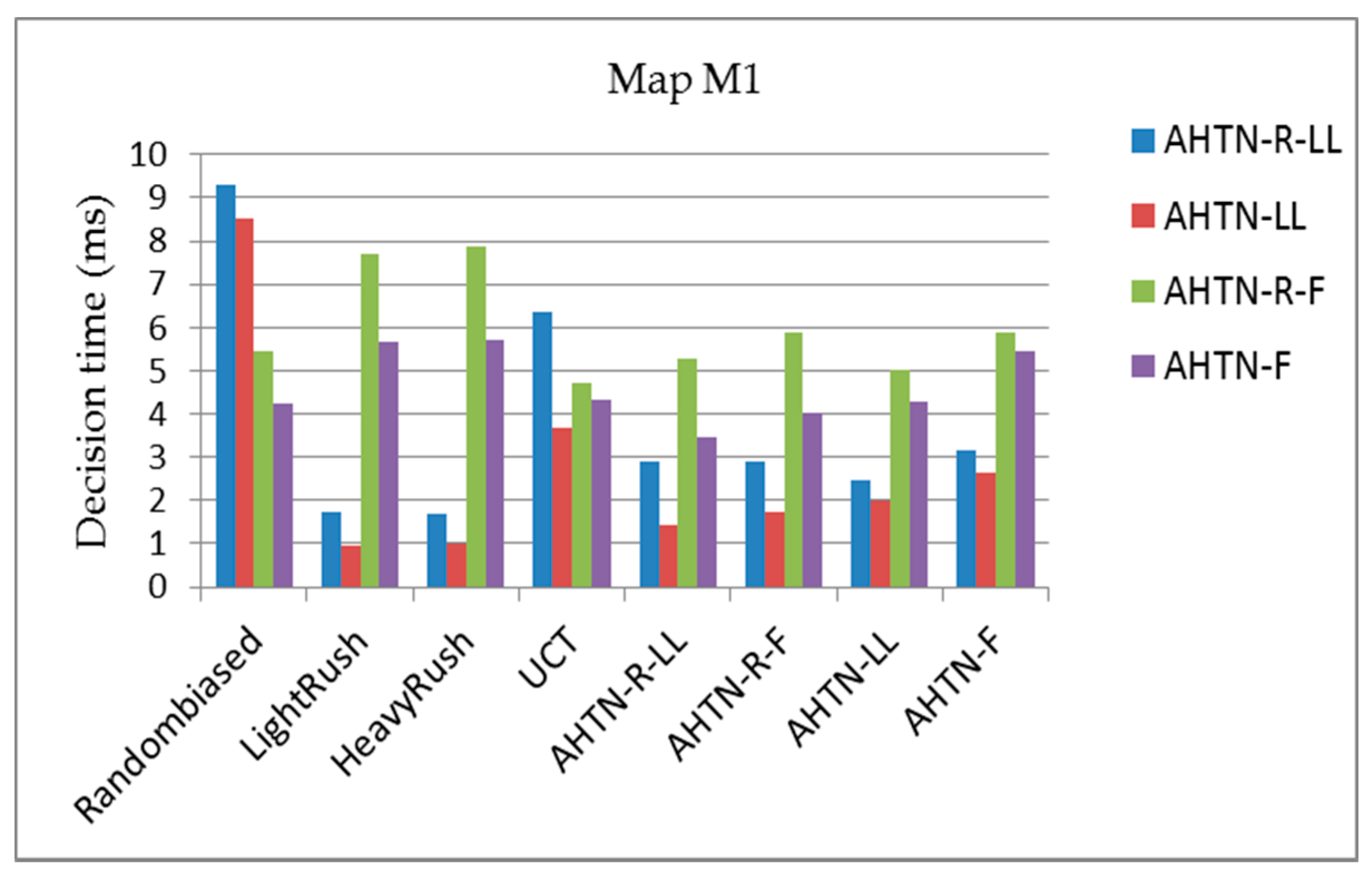
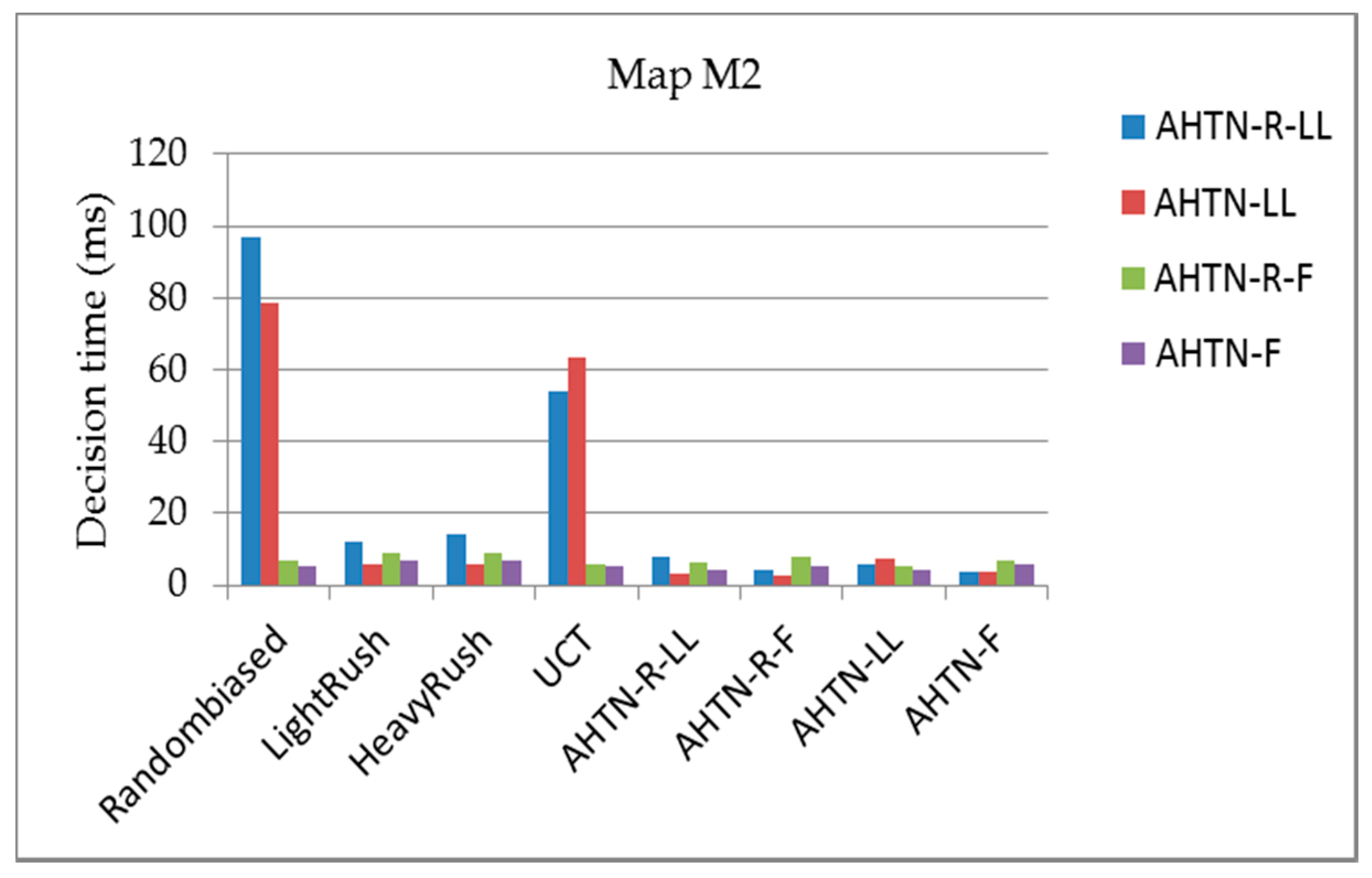
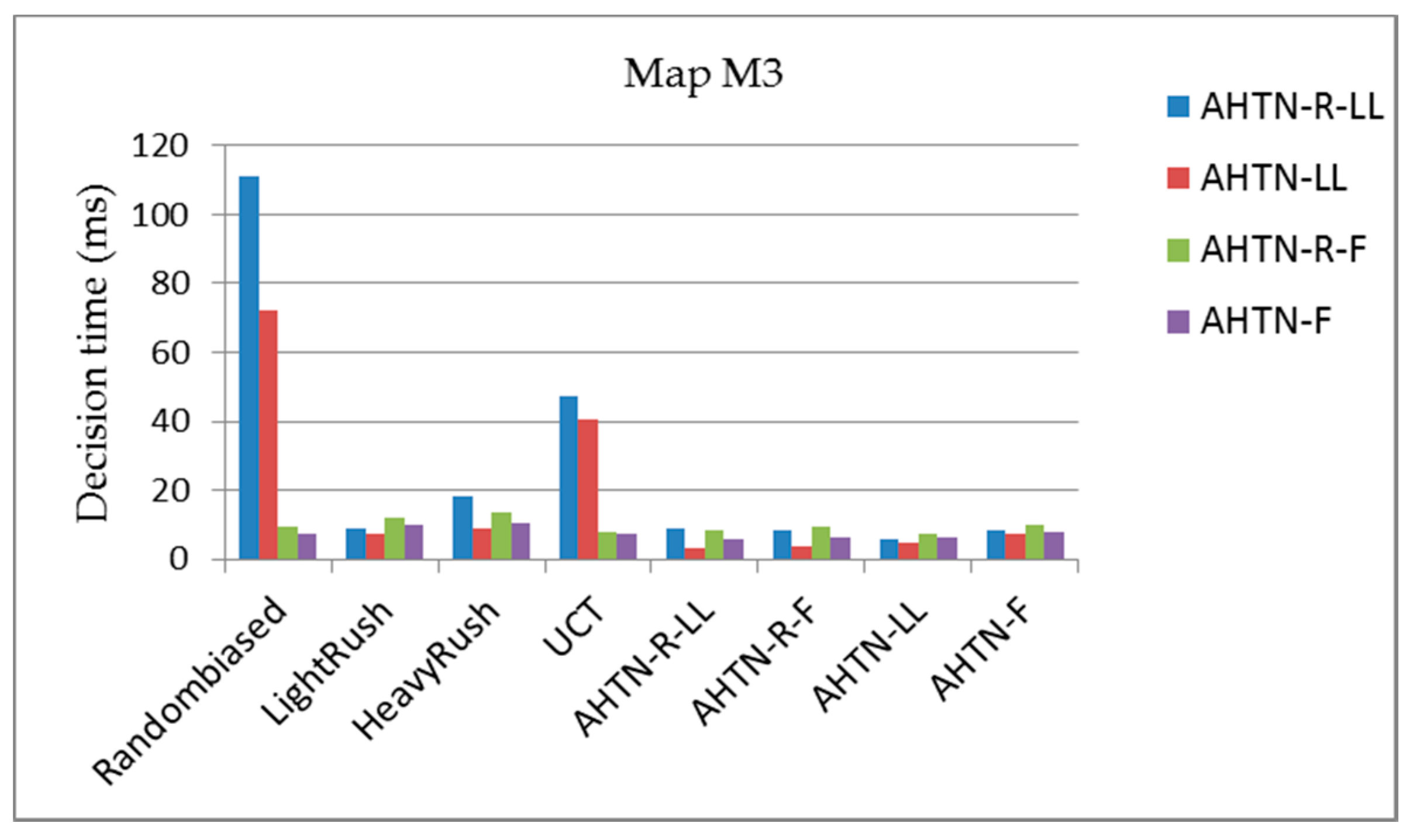
Figure 10, Figure 11 and Figure 12 show the average planning times of the AHTN-R and AHTN players for one decision process of 100 games for the three maps, respectively. We find that AHTN-R usually requires more decision time than AHTN when they have similar domain knowledge. This is caused by the added time of task repair. Both the repair of failed tasks at the beginning of each decision cycle and the sorting of all alternative plans according to their evaluations requires greater planning time for AHTN-R than AHTN. However, as shown in Table 1 and Table 2, the time required for repairing failed tasks and saving alternative plans is short compared with the total time required by the decision process. Therefore, while AHTN-R requires greater decision time than AHTN, it is within an acceptable range. We note that the decision times for AHTN-LL and AHTN-R-LL increase for M2 and M3 when playing against Randombiased or UCT. Compared to the other algorithms, Randombiased and UCT have greater opportunity to create complex game environments due to the greater randomness of their actions. Here, the poor domain knowledge of AHTN-LL and AHTN-R-LL relative to that of AHTN-F and AHTN-R-F makes it more difficult for AHTN-LL and AHTN-R-LL to generate plans in response to the random actions of Randombiased and UCT. Therefore, AHTN-LL and AHTN-R-LL must utilize more recursive tasks in HTN to obtain better solutions. This requires that the AI player search more tree nodes, and the time spent on some nodes also increases with increasing HTN depth.
5.2.3. Average Failed Task Repair Rate for the Three Maps
The average repair rates of AHTN-R against the eight algorithms over 100 games for the three maps are shown in Table 3 and Table 4. We can see that AHTN-R-F has a higher repair rate than AHTN-R-LL against all AI players for all three maps. It is the result of the different levels of domain knowledge used by AHTN-R-LL and AHTN-R-F, where the poor domain knowledge used by AHTN-R-LL was not able to provide good alternative plans for task repair. Here, when a player attempted to repair a failed task, no alternative plans were available due to a lack of units. A greater number of alternative plans with greater differences can increase the repair rate. The improved domain knowledge generated a greater number of alternative plans, which tended to facilitate meeting the requirements of the environment.
6. Conclusions and Future Work
The AHTN algorithm has addressed the problem of very large state spaces and branch factors in RTS games. However, the HTN description employed by AHTN cannot express complex relationships among tasks and accommodate the impacts of the environment. Moreover, the method cannot address task failures caused by dynamic environmental factors during plan execution. Therefore, this paper proposed a modified AHTN algorithm with failed task repair functionality, denoted as AHTN-R, to address these deficiencies in AHTN planning. The main contributions of AHTN-R are as follows.
- (1)
- An extended HTN description employing three additional elements denoted as essential task, phase and exit conditions is introduced to express complex relationships among tasks and accommodate the impacts of the environment.
- (2)
- A monitoring strategy based on the extended HTN description is employed in AHTN-R to identify and terminate all affected tasks localized to the failed task to the greatest extent possible. AHTN-R searches and terminates the affected tasks from the bottom to the top until a parent task has an optional useful method. The strategy is designed to limit the number of tasks affected by the failed task.
- (3)
- A novel task repair strategy based on a prioritized listing of alternative plans is used in AHTN-R to repair failed tasks. In the planning process, AHTN-R saves and sorts all generated plans in the game search tree according to their primary features. When a plan fails, AHTN-R selects the alternative plan with the highest priority from its saved plans to repair the failed task.
For a µRTS game, the AHTN-R obtained the best average score in a round robin competition with standard AHTN and four state-of-the-art search algorithms. In addition, compared with the standard AHTN algorithm, AHTN-R demonstrated its capability for repairing task failures using the extended HTN description to accommodate more complex decision problems with a reasonable degree of increased decision processing time.
In future work, the AHTN-R can be extended in multiple directions. Our experiments demonstrated that the level of domain knowledge of the HTN had a significant influence on the performance of AHTN-R. However, encoding perfect knowledge in an HTN is a difficult and time-consuming process even for domain experts [29]. The automatic extraction of HTNs from thousands of RTS game replays may provide considerable assistance for constructing refined HTNs. In addition, we note that neither AHTN nor AHTN-R consider indetermination and partial observation, which frequently appear in RTS games. This would lead to evolving game states that may differ considerably from the states forecasted during HTN planning, and affect the validity of the plan solution. Some research has been conducted [30,31,32,33,34], but none has been applied in RTS games. Therefore, an improved AHTN-R algorithm using the techniques of HTN planning under uncertainty may enhance its performance in RTS games.
Acknowledgments
We want to thank Santiago Ontanón for discussions about plan repairing. The work described in this paper is sponsored by the National Natural Science Foundation of China under Grant No. 61403402 and No. 61473300.
Author Contributions
Lin Sun, Peng Jiao and Yabing Zha proposed the method; Quanjun Yin, Kai Xu and Lin Sun designed and performed the experiments; Lin Sun and Kai Xu analyzed the experimental data; Lin Sun wrote the paper.
Conflicts of Interest
The authors declare that there is no conflict of interests regarding the publication of this paper.
References
- Buro, M. Real-time strategy games: A new AI research challenge. In Proceedings of the 8th International Joint Conference on Artificial Intelligence, Acapulco, Mexico, 9–15 August 2003; Morgan Kaufmann Publishers Inc.: San Francisco, CA, USA, 2003; pp. 1534–1535. [Google Scholar]
- Ontanón, S.; Synnaeve, G.; Uriarte, A.; Richoux, F.; Churchill, D.; Preuss, M. A survey of real-time strategy game AI research and competition in starcraft. IEEE Trans. Comput. Intell. AI Games 2013, 5, 293–311. [Google Scholar] [CrossRef]
- Knuth, D.E.; Moore, R.W. An analysis of alpha-beta pruning. Artif. Intell. 1975, 6, 293–326. [Google Scholar] [CrossRef]
- Ontañón, S. Experiments with game tree search in real-time strategy games. arXiv, 2012; arXiv:1208.1940. [Google Scholar]
- Chung, M.; Buro, M.; Schaeffer, J. Monte Carlo planning in RTS games. In Proceedings of the 2005 IEEE Symposium on Computational Intelligence and Games (CIG05), Essex University, Colchester, Essex, UK, 4–6 April 2005; pp. 117–172. [Google Scholar]
- Balla, R.K.; Fern, A. UCT for tactical assault planning in real-time strategy games. In Proceedings of the 21st International Jont Conference on Artifical Intelligence, Pasadena, CA, USA, 11–17 July 2009; AAAI Press: Palo Alto, CA, USA, 2009; pp. 40–45. [Google Scholar]
- Churchill, D.; Saffidine, A.; Buro, M. Fast Heuristic Search for RTS Game Combat Scenarios. In Proceedings of the Artificial Intelligence and Interactive Digital Entertainment (AIIDE), Stanford, CA, USA, 8–12 October 2012. [Google Scholar]
- Ontanón, S. The combinatorial multi-armed bandit problem and its application to real-time strategy games. In Proceedings of the 9th Artificial Intelligence and Interactive Digital Entertainment Conference (AIIDE), Boston, MA, USA, 14–18 October 2013. [Google Scholar]
- Shleyfman, A.; Komenda, A.; Domshlak, C. On combinatorial actions and CMABs with linear side information. In Proceedings of the 21st European Conference on Artificial Intelligence, Prague, Czech Republic, 18–22 August 2014. [Google Scholar]
- Ontanón, S.; Buro, M. Adversarial hierarchical-task network planning for complex real-time games. In Proceedings of the 24th International Conference on Artificial Intelligence, Buenos Aires, Argentina, 25–31 July 2015; AAAI Press: Palo Alto, CA, USA, 2015. [Google Scholar]
- Sacerdoti, E.D. The nonlinear nature of plans. In Proceedings of the 4th International Joint Conference on Artificial Intelligence, Tblisi, Georgia, 3–8 September 1975; No. SRI-TN-101. Morgan Kaufmann Publishers Inc.: San Francisco, CA, USA, 1975. [Google Scholar]
- Nau, D.; Cao, Y.; Lotem, A.; Muftoz-Avila, H. SHOP: Simple hierarchical ordered planner. In Proceedings of the 16th International Joint Conference on Artificial Intelligence-Volume 2, Stockholm, Sweden, 31 July–6 August 1999; Morgan Kaufmann Publishers Inc.: San Francisco, CA, USA, 1999; pp. 968–973. [Google Scholar]
- Nau, D.S.; Ilghami, O.; Kuter, U.; Murdock, J.W.; Wu, D.; Yaman, F. SHOP2: An HTN planning system. J. Artif. Intell. Res. 2003, 20, 379–404. [Google Scholar]
- Kelly, J.-P.; Botea, A.; Koenig, S. Planning with hierarchical task networks in video games. In Proceedings of the ICAPS-07 Workshop on Planning in Games, Providence, RI, USA, 22–26 September 2007. [Google Scholar]
- Menif, A.; Jacopin, E.; Cazenave, T. SHPE: HTN Planning for Video Games. In Proceedings of the Third Workshop on Computer Games, Prague, Czech Republic, 18 August 2014. [Google Scholar]
- Soemers, D.J.N.J.; Winands, M.H.M. Hierarchical Task Network Plan Reuse for Video Games. In Proceedings of the 2016 IEEE Conference on Computational Intelligence and Games (CIG), Santorini, Greece, 20–23 September 2016. [Google Scholar]
- Humphreys, T. Exploring HTN planners through examples. In Game AI Pro: Collected Wisdom of Game AI Professionals; A K Peters, Ltd.: Natick, MA, USA, 2013; pp. 149–167. [Google Scholar]
- Muñoz-Avila, H.; Aha, D. On the role of explanation for hierarchical case-based planning in real-time strategy games. In Proceedings of the ECCBR-04 Workshop on Explanations in CBR, Madrid, Spain, 30 August–2 September 2004; Springer: Berlin, Germany, 2004. [Google Scholar]
- Spring RTS. Available online: http://springrts.com (accessed on 1 February 2016).
- Laagland, J. A HTN Planner for a Real-Time Strategy Game. 2014. Available online: http://hmi.ewi.utwente.nl/verslagen/capita-selecta/CS-Laagland-Jasper.pdf (accessed on 20 October 2015).
- Naveed, M.; Kitchin, D.E.; Crampton, A. A hierarchical task network planner for pathfinding in real-time strategy games. In Proceedings of the Third International Symposium on AI & Games, Leicester, UK, 29 March–1 April 2010. [Google Scholar]
- Sánchez-Garzón, I.; Fdez-Olivares, J.; Castillo, L. A Repair-Replanning Strategy for HTN-Based Therapy Planning Systems. 2011. Available online: https://decsai.ugr.es/~faro/LinkedDocuments/FinalSubmission_DC_AIME11.pdf (accessed on 5 October 2015).
- Gateau, T.; Lesire, C.; Barbier, M. Hidden: Cooperative plan execution and repair for heterogeneous robots in dynamic environments. In Proceedings of the 2013 IEEE/RSJ International Conference on Intelligent Robots and Systems, Tokyo, Japan, 3–7 November 2013; IEEE: Piscataway, NJ, USA, 2013. [Google Scholar]
- Ayan, N.F.; Kuter, U.; Yaman, F.; Goldman, R.P. Hotride: Hierarchical ordered task replanning in dynamic environments. In Proceedings of the 3rd Workshop on Planning and Plan Execution for Real-World Systems, Providence, RI, USA, 22–26 September 2007. [Google Scholar]
- Erol, K.; Hendler, J.A.; Nau, D.S. UMCP: A Sound and Complete Procedure for Hierarchical Task-network Planning. In Proceedings of the Second International Conference on Artificial Intelligence Planning Systems, Chicago, IL, USA, 13–15 June 1994. [Google Scholar]
- Lin, S. AHTN-R. Available online: https://github.com/mksl163/AHTN-R (accessed on 20 August 2017).
- Ontañón, S. microRTS. 2016. Available online: https://github.com/santiontanon/microrts (accessed on 22 February 2016).
- Churchill, D.; Buro, M. Portfolio greedy search and simulation for large scale combat in StarCraft. In Proceedings of the 2013 IEEE Conference Computational Intelligence in Games (CIG), Niagara Falls, ON, Canada, 11–13 August 2013; IEEE: Piscataway, NJ, USA, 2013; pp. 1–8. [Google Scholar]
- Zhuo, H.H.; Hu, D.H.; Hogg, C.; Yang, Q.; Munoz-Avila, H. Learning HTN method preconditions and action models from partial observations. In Proceedings of the 21st International Jont Conference on Artifical Intelligence, Pasadena, CA, USA, 11–17 July 2009; Morgan Kaufmann Publishers Inc.: San Francisco, CA, USA, 2009; pp. 1804–1810. [Google Scholar]
- Kuter, U.; Nau, D. Forward-chaining planning in nondeterministic domains. In Proceedings of the 19th National Conference on Artifical Intelligence, San Jose, CA, USA, 25–29 July 2004; AAAI Press: Palo Alto, CA, USA, 2004. [Google Scholar]
- Kuter, U.; Nau, D. Using domain-configurable search control for probabilistic planning. In Proceedings of the National Conference on Artificial Intelligence, Pittsburgh, PA, USA, 9–13 July 2005; AAAI Press: Palo Alto, CA, USA, 2005; pp. 1169–1174. [Google Scholar]
- Bonet, B.; Geffner, H. Planning with incomplete information as heuristic search in belief space. In Proceedings of the 5th International Conference on Artificial Intelligence Planning Systems, Breckenridge, CO, USA, 14–17 April 2000; AAAI Press: Palo Alto, CA, USA, 2000; pp. 52–61. [Google Scholar]
- Bonet, B.; Geffner, H. Labeled RTDP: Improving the Convergence of Real-Time Dynamic Programming. In Proceedings of the Thirteenth International Conference on Automated Planning and Scheduling, Trento, Italy, 9–13 June 2003; AAAI Press: Palo Alto, CA, USA, 2003; Volume 3. [Google Scholar]
- Bertsekas, D.P. Dynamic Programming and Optimal Control; Athena Scientific: Belmont, MA, USA, 1995; Volume 1. [Google Scholar]
Figure 1.
An example of the ambushing-enemy task.
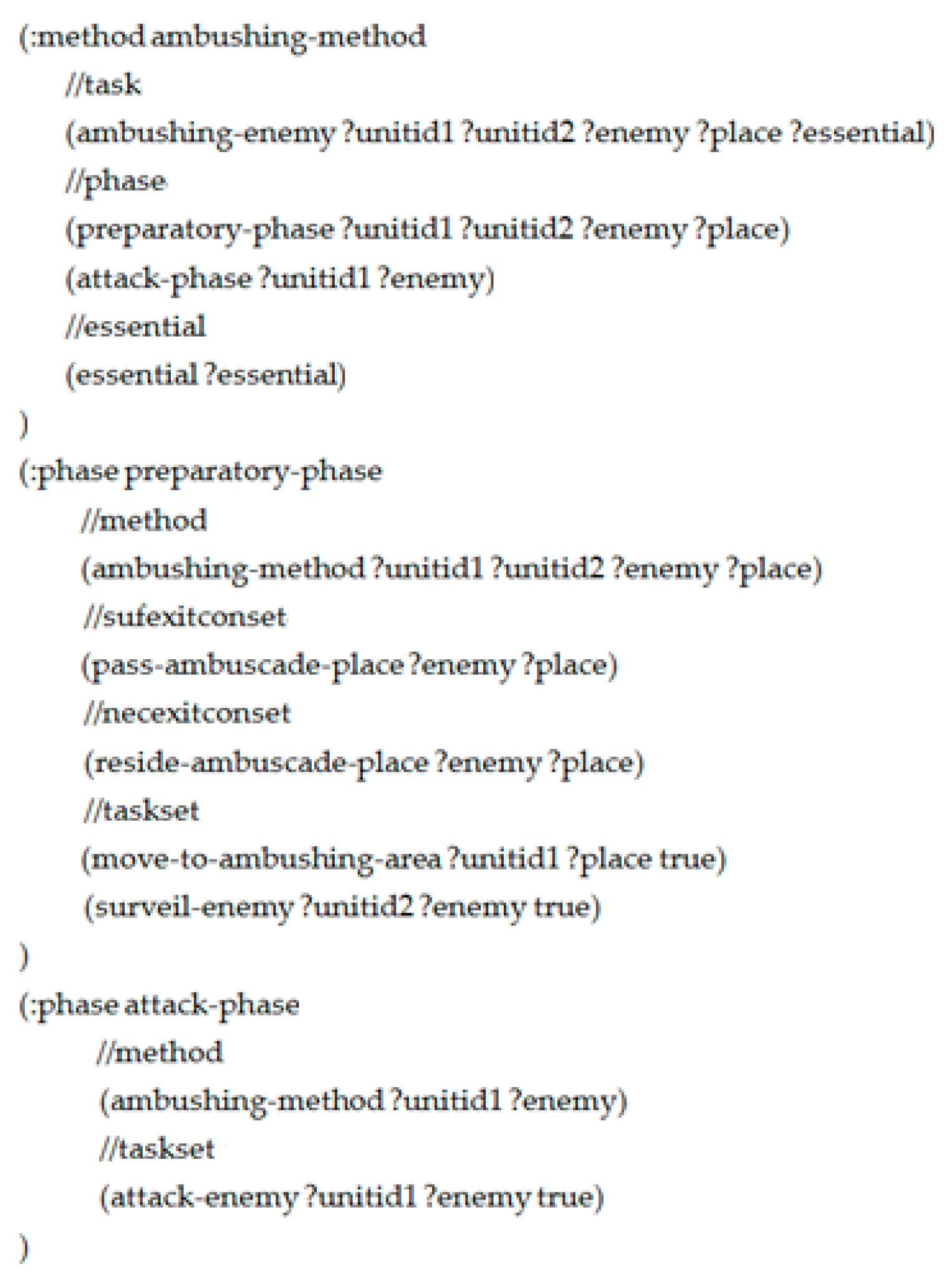
Figure 2.
Overall framework of the adversarial hierarchical task network (AHTN)-R algorithm.
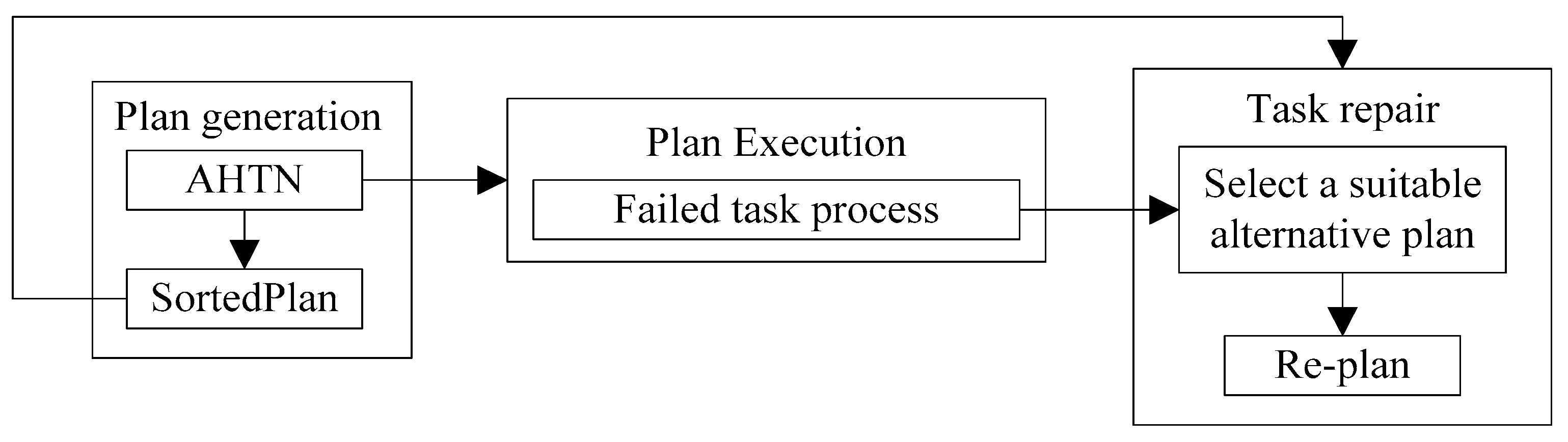
Figure 3.
A min–max search tree is employed as an example for proof of Theorem 1. The rectangular nodes are max nodes, which are ordered increasingly from left to right according to their evaluations, and the circular nodes are min nodes, which are ordered decreasingly from left to right according to their evaluations.

Figure 4.
An Example of repairing a failed plan (a) owing to the failure of subtask T6 by employing an alternative plan (b).
Figure 4.
An Example of repairing a failed plan (a) owing to the failure of subtask T6 by employing an alternative plan (b).

Figure 5.
A screenshot of the µRTS game environment. The two players are distinguished according to the blue and red outline colors. The green squares are resources. The white squares are bases. The gray circles are workers, the yellow circles are heavy attackers, and the orange circles are light attackers.
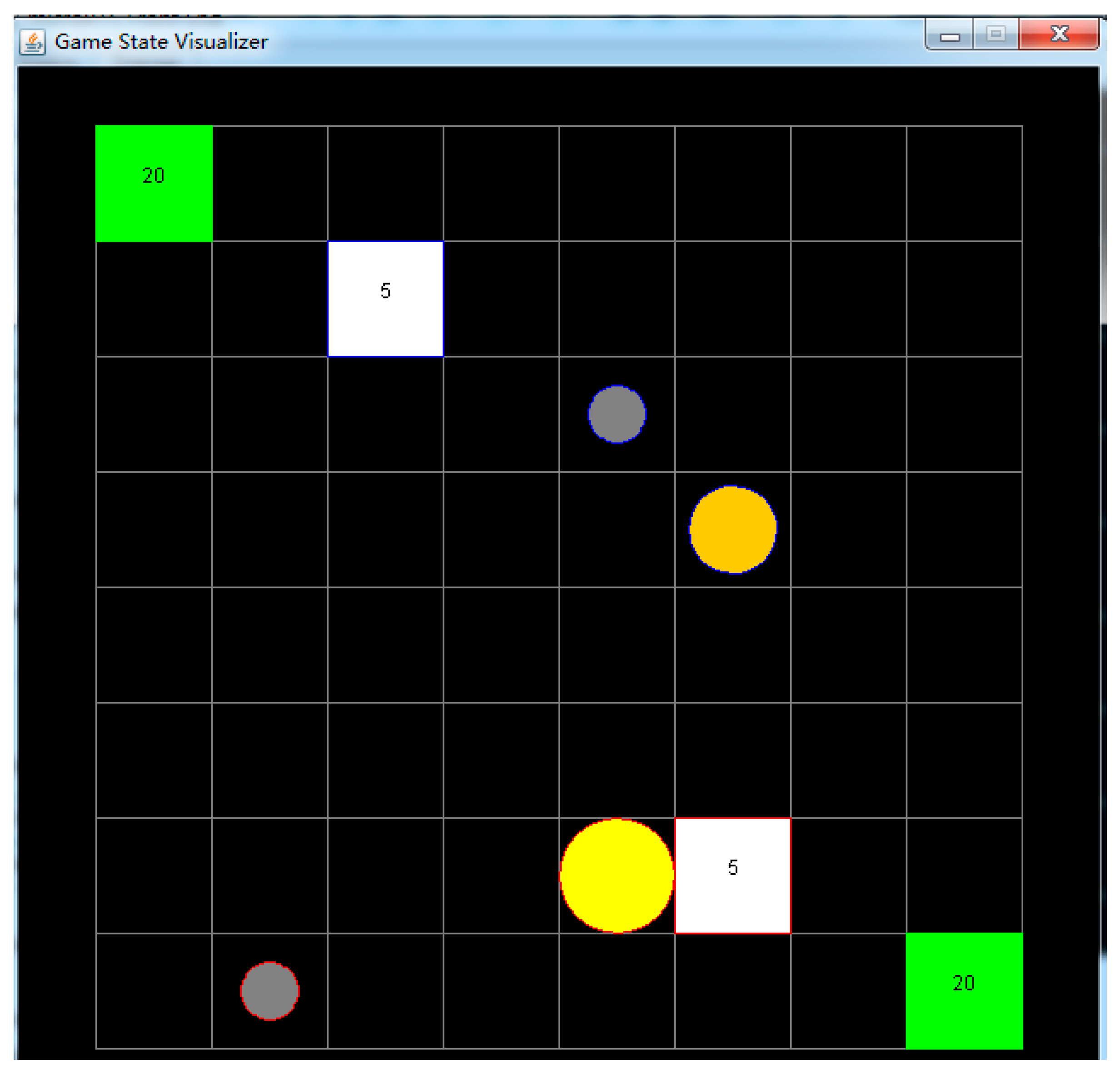
Figure 6.
An example of the AHTN-R process of executing the compound task destroy-player-internal from the Low-Level functionality.
Figure 6.
An example of the AHTN-R process of executing the compound task destroy-player-internal from the Low-Level functionality.
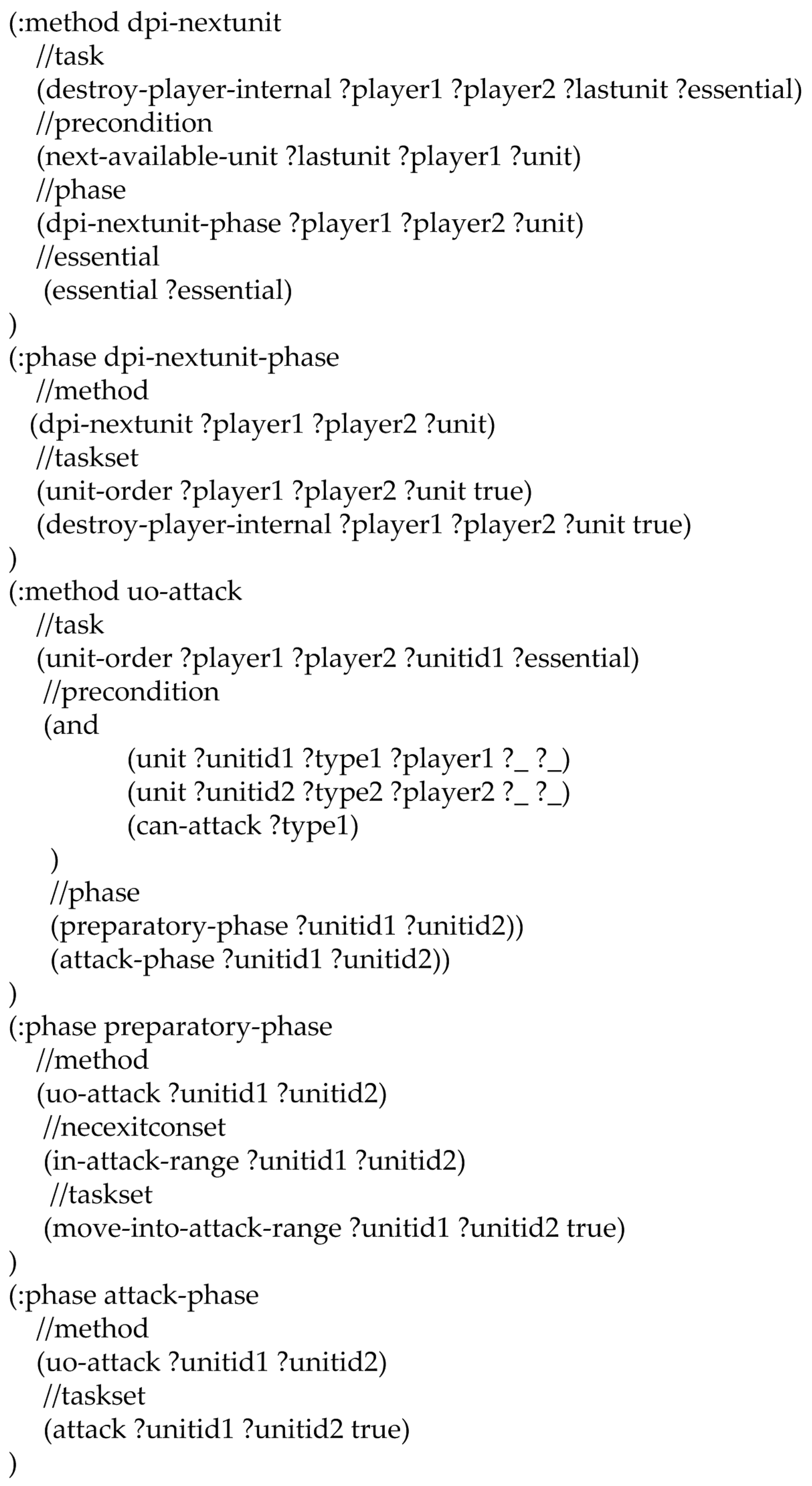
Figure 7.
The average score of each algorithm obtained over the 800 games of the round-robin competition for map M1 (8 × 8 tiles) with respect to the CPU time from 20 to 200 ms. The playout time is 100 cycles.
Figure 7.
The average score of each algorithm obtained over the 800 games of the round-robin competition for map M1 (8 × 8 tiles) with respect to the CPU time from 20 to 200 ms. The playout time is 100 cycles.

Figure 8.
The average score of each algorithm obtained over the 800 games of the round-robin competition for map M2 (12 × 12 tiles) with respect to the CPU time from 20 to 200 ms. The playout time is 100 cycles.
Figure 8.
The average score of each algorithm obtained over the 800 games of the round-robin competition for map M2 (12 × 12 tiles) with respect to the CPU time from 20 to 200 ms. The playout time is 100 cycles.

Figure 9.
The average score of each algorithm obtained over the 800 games of the round-robin competition for map M3 (16 × 16 tiles) with respect to the CPU time from 20 to 200 ms. The playout time is 100 cycles.
Figure 9.
The average score of each algorithm obtained over the 800 games of the round-robin competition for map M3 (16 × 16 tiles) with respect to the CPU time from 20 to 200 ms. The playout time is 100 cycles.

Figure 10.
The average decision times of AHTN-R and AHTN with the two types of HTNs obtained over 100 games against each of the 8 algorithms, where the CPU time is 100 ms for map M1 (8 × 8 tiles). The playout time is 100 cycles.
Figure 10.
The average decision times of AHTN-R and AHTN with the two types of HTNs obtained over 100 games against each of the 8 algorithms, where the CPU time is 100 ms for map M1 (8 × 8 tiles). The playout time is 100 cycles.

Figure 11.
The average decision times of AHTN-R and AHTN with the two types of HTNs obtained over 100 games against each of the 8 algorithms, where the CPU time is 100 ms for map M2 (12 × 12 tiles). The playout time is 100 cycles.
Figure 11.
The average decision times of AHTN-R and AHTN with the two types of HTNs obtained over 100 games against each of the 8 algorithms, where the CPU time is 100 ms for map M2 (12 × 12 tiles). The playout time is 100 cycles.

Figure 12.
The average decision times of AHTN-R and AHTN with the two types of HTNs obtained over 100 games against each of the 8 algorithms, where the CPU time is 100 ms for map M3 (16 × 16 tiles). The playout time is 100 cycles.
Figure 12.
The average decision times of AHTN-R and AHTN with the two types of HTNs obtained over 100 games against each of the 8 algorithms, where the CPU time is 100 ms for map M3 (16 × 16 tiles). The playout time is 100 cycles.


Table 1.
The percentage of extra time required for repairing failed tasks and saving alternative plans relative to the total time for decision processing. The games were between AHTN-R-LL and the 8 algorithms for the three map sizes (M1 is 8 × 8 tiles, M2 is 12 × 12 tiles, and M3 is 16 × 16 tiles).
Table 1.
The percentage of extra time required for repairing failed tasks and saving alternative plans relative to the total time for decision processing. The games were between AHTN-R-LL and the 8 algorithms for the three map sizes (M1 is 8 × 8 tiles, M2 is 12 × 12 tiles, and M3 is 16 × 16 tiles).
| AI Player | M1 | M2 | M3 |
|---|---|---|---|
| Randombiased | 0.1682 | 0.0003 | 0.0003 |
| LightRush | 0.0381 | 0.0078 | 0.0105 |
| HeavyRush | 0.0355 | 0.0066 | 0.0070 |
| UCT | 0.0498 | 0.0057 | 0.0060 |
| AHTN-R-LL | 0.0202 | 0.0128 | 0.0137 |
| AHTN-R-F | 0.034 | 0.0188 | 0.0103 |
| AHTN-LL | 0.0221 | 0.0103 | 0.0114 |
| AHTN-F | 0.0176 | 0.0174 | 0.0071 |
Table 2.
The percentage of extra time required for repairing failed tasks and saving alternative plans relative to the total time for decision processing. The games were between AHTN-R-F and the 8 algorithms for the three map sizes.
Table 2.
The percentage of extra time required for repairing failed tasks and saving alternative plans relative to the total time for decision processing. The games were between AHTN-R-F and the 8 algorithms for the three map sizes.
| AI Player | M1 | M2 | M3 |
|---|---|---|---|
| Randombiased | 0.0265 | 0.0290 | 0.0228 |
| LightRush | 0.0226 | 0.0259 | 0.0217 |
| HeavyRush | 0.0216 | 0.0275 | 0.0219 |
| UCT | 0.027 | 0.0274 | 0.0275 |
| AHTN-R-LL | 0.0312 | 0.0348 | 0.0391 |
| AHTN-R-F | 0.0302 | 0.0353 | 0.0272 |
| AHTN-LL | 0.0232 | 0.0279 | 0.0283 |
| AHTN-F | 0.0192 | 0.0263 | 0.0141 |
Table 3.
Average repair rate of AHTN-R-LL against the 8 algorithms for the three map sizes. The symbol “-” indicates no failed tasks.
Table 3.
Average repair rate of AHTN-R-LL against the 8 algorithms for the three map sizes. The symbol “-” indicates no failed tasks.
| AI Player | M1 | M2 | M3 |
|---|---|---|---|
| Randombiased | 0.262 | 0.278 | 0.227 |
| LightRush | - | 0.324 | 0.037 |
| HeavyRush | - | 0.929 | 0 |
| UCT | 0.618 | 0.591 | 0.553 |
| AHTN-R-LL | 0 | 0 | 0 |
| AHTN-R-F | 0.005 | 0 | 0 |
| AHTN-LL | 0.355 | 0.343 | 0.373 |
| AHTN-F | 0.236 | 0.233 | 0.213 |
Table 4.
Average repair rate of AHTN-R-F against the 8 algorithms for the three map sizes. The symbol “-” indicates no failed tasks.
Table 4.
Average repair rate of AHTN-R-F against the 8 algorithms for the three map sizes. The symbol “-” indicates no failed tasks.
| AI Player | M1 | M2 | M3 |
|---|---|---|---|
| Randombiased | 0.904 | 0.886 | 0.852 |
| LightRush | - | 0.753 | 0.449 |
| HeavyRush | 1 | 1 | 0.767 |
| UCT | 0.945 | 0.907 | 0.906 |
| AHTN-R-LL | 0.008 | 0.044 | 0 |
| AHTN-R-F | 0.016 | 0.01 | 0.018 |
| AHTN-LL | 0.401 | 0.618 | 0.697 |
| AHTN-F | 0.407 | 0.373 | 0.452 |
© 2017 by the authors. Licensee MDPI, Basel, Switzerland. This article is an open access article distributed under the terms and conditions of the Creative Commons Attribution (CC BY) license (http://creativecommons.org/licenses/by/4.0/).
Share and Cite
MDPI and ACS Style
Sun, L.; Jiao, P.; Xu, K.; Yin, Q.; Zha, Y. Modified Adversarial Hierarchical Task Network Planning in Real-Time Strategy Games. Appl. Sci. 2017, 7, 872. https://doi.org/10.3390/app7090872
AMA Style
Sun L, Jiao P, Xu K, Yin Q, Zha Y. Modified Adversarial Hierarchical Task Network Planning in Real-Time Strategy Games. Applied Sciences. 2017; 7(9):872. https://doi.org/10.3390/app7090872
Chicago/Turabian StyleSun, Lin, Peng Jiao, Kai Xu, Quanjun Yin, and Yabing Zha. 2017. "Modified Adversarial Hierarchical Task Network Planning in Real-Time Strategy Games" Applied Sciences 7, no. 9: 872. https://doi.org/10.3390/app7090872
Note that from the first issue of 2016, this journal uses article numbers instead of page numbers. See further details here.