Real-time Monitoring for Disk Laser Welding Based on Feature Selection and SVM

1
School of Computer, South China Normal University, Guangzhou 510631, China
2
School of Electromechanical Engineering, Guangdong University of Technology, Guangzhou 510090, China
3
College of Information Science and Engineering, Central South University, Changsha 410083, China
*
Author to whom correspondence should be addressed.
Appl. Sci. 2017, 7(9), 884; https://doi.org/10.3390/app7090884
Submission received: 26 July 2017
/
Revised: 25 August 2017
/
Accepted: 25 August 2017
/
Published: 28 August 2017
Abstract
:In order to automatically evaluate the welding quality during high-power disk laser welding, a real-time monitoring system was developed. The images of laser-induced metal vapor during welding were captured and fifteen features were extracted. A feature selection method based on a sequential forward floating selection algorithm was employed to identify the optimal feature subset, and a support vector machine (SVM) classifier was built to recognize the welding quality. The experiment results demonstrated that this method had satisfactory performance, and could be applied in laser welding monitoring applications.
PACS:
81.20.Vj; 89.20.Kk
1. Introduction
Because of its high production quality, laser welding has become one of the most important welding techniques in the modern manufacturing industry [1,2]. However, compared to traditional welding technologies, the energy transmission during laser welding is complex and unstable, which makes it a formidable challenge to monitor the laser welding process. Therefore, developing effective and accurate monitoring methods is of great importance in guaranteeing process stability and the product quality.
Video cameras offer the unique capability of collecting high-density spatial data from a distant scene of interest. They can be employed as remote monitoring or inspection sensors for structures. Cha et al. [3] have done a lot of research work in the field to advance the methodology towards the eventual goal of using a camera as a sensor for the detection and assessment of structures. They propose some novel vision-based methods using a deep architecture of convolutional neural networks for detecting loosened bolts [3] and concrete cracks [4]. Geometric features varying three dimensionally are extracted from two-dimensional images taken by the camera [3,4]. They have demonstrated motion magnification for extracting displacements from the high-speed video [4], and demonstrated the algorithm’s capability to qualitatively identify the operational deflection shapes of a cantilever beam and a pipe cross section from a video [5,6]. Furthermore, new damage detection methodologies have been proposed by integrating a nonlinear recursive filter [6] and using a density peaks-based fast clustering algorithm; damage-sensitive features are extracted from the measured data through a non-contact computer vision system [7].
Computer-aided analysis techniques have been widely applied to monitor manufacturing processes [8,9]. Especially since their recent rapid development, machine learning and pattern recognition methods have attracted considerable attention. Wan et al. [10] developed an efficient quality monitoring system for small scale resistance spot welding based on dynamic resistance. A back propagation neural network was used to estimate the weld quality, and showed a better performance than regression analysis. Casalino et al. [11] investigated the main effects of process parameters on laser welding process quality. An artificial neural network model was built to forecast the features of the welding bead. Experiment results showed that the neural network was able to predict with significant accuracy.
Support vector machines (SVM) are a practical method for classification and regression. It is motivated by the statistical learning theory developed by Vapnik et al. [12,13], and has been successfully applied to a number of applications in the welding industry. Liu et al. [14] explored the relationship between the welding process and welded quality. A multiple sensor fusion system was built to obtain the photodiode and visible light information, and SVM was used to classify three types of weld quality. Experiment results showed that the estimation on welding status was accurate. Fan et al. [15] developed an automatic recognition system for welding seam types; an SVM-based modeling method was used to achieve welding seam type recognition accurately. Mekhalfa and Nacereddine [16] used SVM to automatically classify four types of weld defects in radiographic images. Nevertheless, the performance of SVM is highly affected by the features used. Lack of precise a priori knowledge, and selecting features blindly may lead to unsatisfactory classification accuracy.
In this work, three welding experiments were conducted at different welding speeds using high-power disk laser. The images of laser-induced metal vapor during welding were captured by a high-speed camera. Fifteen features of the metal vapor plume and spatters were extracted from each image. A feature selection method was employed to identify the optimal feature subset, and an SVM classifier was built to evaluate the welding quality automatically. The back-propagation neural network was used as a comparison, and the experiment results showed that, with an appropriate feature selection method, the SVM classifier can achieve higher accuracy.
2. Methods
2.1. Support Vector Machine (SVM)
Given a binary classification task with datapoints (i = 1, ..., N) and corresponding labels . Each datapoint represents a d-dimensional input.
Assuming that the given datapoints are linearly separable, there exist hyperplanes that correctly separate all the points. The SVM method attempts to identify these separating hyperplanes. The definition for the separating hyperplane in multidimensional space is:
The vector w determines the orientation of the discriminant plane and the scalar b determines the offset of the hyperplane from the origin.
The margin between two classes determines the generalization ability of a separating hyperplane; therefore, the support vector algorithm simply looks for the separating hyperplane with the largest margin. While the margin of a separating hyperplane is calculated as , where is the Euclidean norm of w, the problem can be formulated as:
As a constrained optimization problem, the Lagrange multiplier vector is introduced and the Lagrange function is:
Then the primal optimization problem can be rewritten as the dual problem:
In most cases, outliers exist, which means the data set is linearly separable when a few data points are removed. The SVM method tolerates these outliers by adding the penalty factor C and changing the dual problem to:
C determines the punishment for the outliers.
This is a convex quadratic programming problem, and there are many effective robust algorithms for solving it. The solution can be used to calculate and . Then, the optimal separating hyperplane is:
and the SVM classification function is:
The method above is called linear SVM, which assumes the training data set is linearly separable (or almost linearly separable), and that a linear separating surface can be found. But in many cases, the datapoints are not linearly separable, and the function of the optimal separating surface may be nonlinear. By using a method called kernel trick, the SVM method can be extended to handle this kind of problem. The main idea is mapping the input data onto a higher dimensional space called feature space and then performing linear classification there. This can be done implicitly by replacing the inner product with kernel function.
Several kernel functions have been explored, such as polynomial kernels, sigmoid kernels and radial basis function (RBF) kernels. The RBF kernel is one of the most widely applied kernel functions, usually in its Gaussian form:
The parameter σ determines the radial range of the function.
Generally, the performance of the RBF kernel is satisfactory, and the parameter setting is relatively simple, thus the RBF kernel is applied in this study.
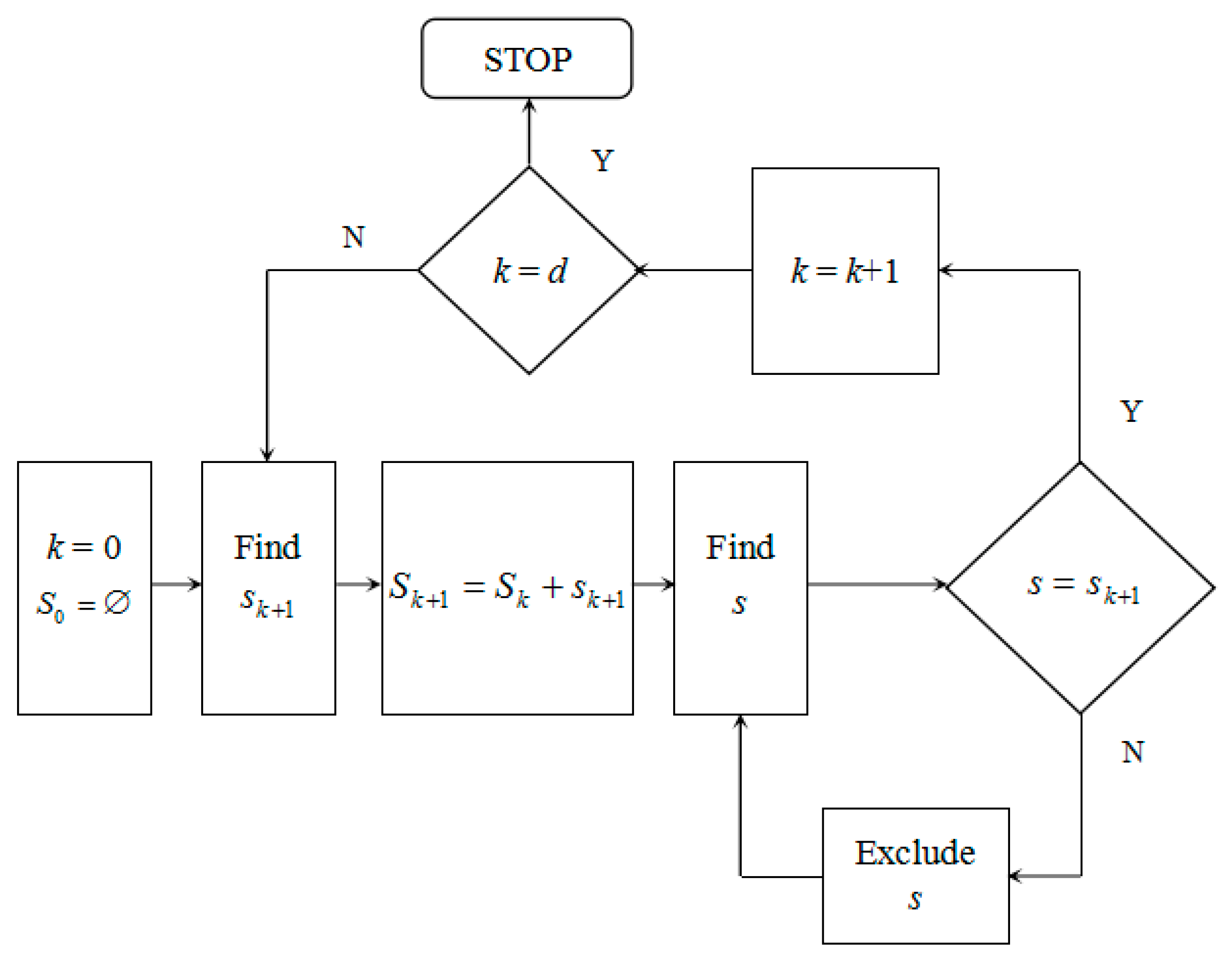
2.2. Sequential Forward Floating Selection
The main goal of feature selection is to select a subset of d features from the original data set of D features (d < D) according to a certain evaluation criterion and improve the performance of the pattern recognition system, such as higher classification accuracy, lower computational cost and better model interpretability.
Assuming that a suitable evaluation criterion function has been chosen, feature selection is reduced to a search problem that detects an optimal feature subset based on the selected measure. Many search strategies have been designed to avoid the exhaustive search even though the feature set obtained may be suboptimal. The sequential forward floating selection (SFFS) algorithm is a relatively new strategy, and has been widely applied in practice [20,21,22].
Suppose k features have already been selected from the original data set to form set with the corresponding criterion function . The search procedure includes two basic steps:
- Step 1 (Inclusion). Select the best feature from the set of available features :and add to . Therefore:
- Step 2 (Exclusion). Find the worst feature s in the set :and if , set and return to Step 1; if not, exclude s from and execute Step 2 again.
The algorithm is usually initialized by setting and , and run until a set of d features is obtained. The flow chart of SFFS algorithm is shown in Figure 1.
3. Experiment
3.1. Disk Laser Welding
The experiment was performed by using a high-power disk laser TruDisk 10003 (TRUMPF, Ditzingen, Germany), and high-speed camera system Memrecam fx RX6 (NAC, Tokyo, Japan). The beam diameter of the disk laser focus was 480 µm, while the laser wavelength was 1030 nm and the laser power was 10 kW. Argon was used as a shielding gas, and the nozzle angle was 45°. Type 304 stainless steel with dimensions of 119 × 51 × 20 mm was employed as the specimen. Three different welding speeds, 3, 4.5 and 6 m/min, were taken into consideration in this experiment (see Table 1). The high-speed camera was setup at a position perpendicular to the welding direction to capture the images of plume and spatters. The frame rate was 2000 f/s, and the image resolution was 512 × 512 pixels. An optical filter was placed in front of the RX6 to reduce the effect of multiple reflections.
3.2. Image Processing
The goal of image processing is to filter unnecessary information and identify the region of interest (ROI) from the original image. As this is the fundamental basis for feature extraction and other further analysis, it plays a very important role in a pattern recognition system. Many image processing techniques have been developed [25], such as filtering, morphology and image segmentation.
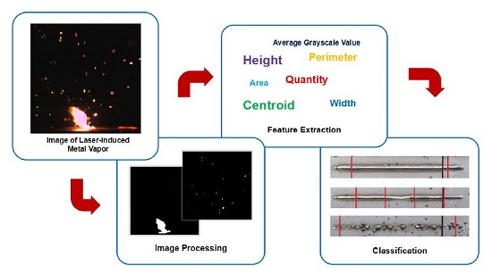
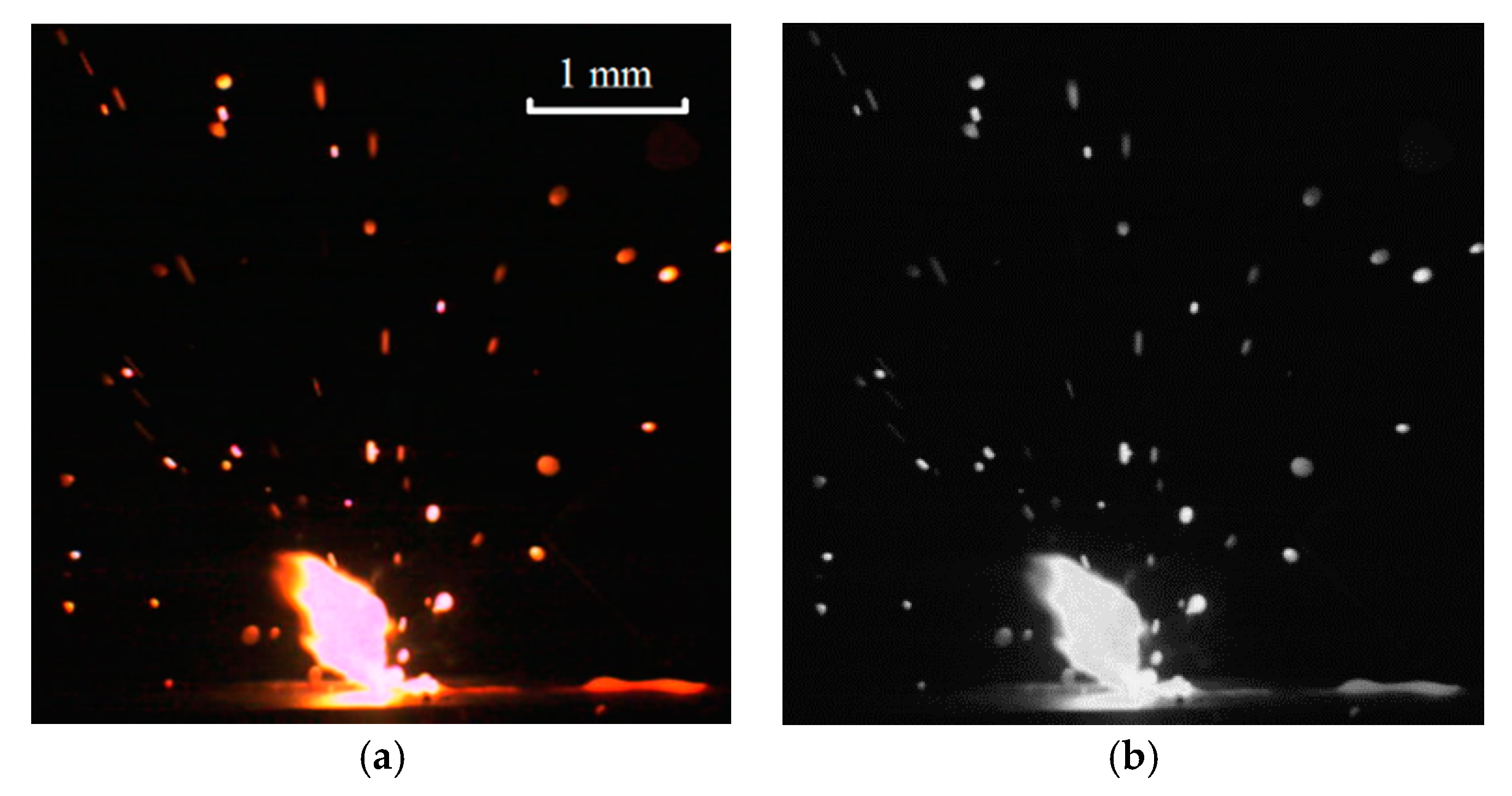
The RGB color image (Figure 2a) captured by the high-speed camera was first converted to grayscale to emphasize morphological characteristics and reduce computational consumption. Then the grayscale image (Figure 2b) was segmented by thresholding to generate the binary images of plume and spatters; all points with grayscale value greater than 183 were regarded as regions of the plume and spatters, and others were background. After that, the binary image of plume (Figure 2c) was obtained by deleting the regions with area smaller than 400 pixels; the binary image of spatters (Figure 2d) was the logical symmetric difference of the two binary images above.
3.3. Feature Extraction
Feature extraction attempts to generate informative and non-redundant derived values from the initial measured data. As this facilitates the subsequent classifier generation, and usually leads to a better understanding of the problem, it is considered to be a critical step in a pattern recognition system. In this study, fifteen features (see Table 2) are extracted from the image of plume and spatters. Their definitions are as follows [26].
Area: The area is calculated by counting the number of white points in the binary image. The area of plume is denoted Ap, and the sum of all areas of spatters is denoted As.
Perimeter: In the binary image, the points surrounded by difference colors are marked as boundary points, and the number of boundary points is taken as the perimeter. The perimeter of plume is denoted Pp, and the sum of all perimeters of spatters is denoted Ps.
Centroid: The centroid (i, j) of plume and the centroid (i, j) of spatters are calculated by:
where g(i, j) is the grayscale value of the point (i, j). They are denoted Cp(i), Cp(j), Cs(i) and Cs(j).
Height: The height of plume is the vertical distance between the highest point and the lowest point, which is denoted Hp.
Width: The width of plume is the horizontal distance between the far-left point and the far-right point, which is denoted Wp.
Average Grayscale Value: The average grayscale value of plume and the average grayscale value of spatters are calculated by:
where g(i, j) is the grayscale value of the point (i, j). They are denoted Gp and Gs.
Quantity: The quantity of spatters is defined as the number of connected objects found in the binary image of spatters. Three different quantities are used in this work. The quantity of spatters in the whole image is first calculated and denoted as Qs(a). Then the image is cut vertically into two images of the same size from the middle. Two more quantities are calculated based on these, and denoted Qs(l) and Qs(r).
Features on different scales may cause some problems while evaluating their contributions and optimizing the classifier. Consequently, all extracted features are normalized by the following formula:
where is the No. of the feature, is the normalized data, is the original data, are the minimum values of each feature, and are the maximum values of each feature.
3.4. Feature Selection and Classification
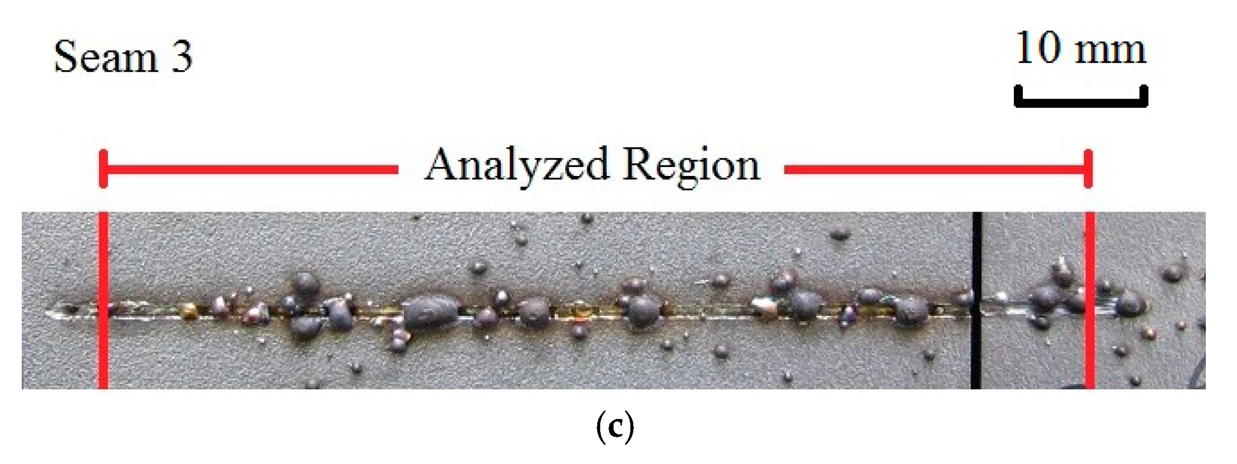
In this study, three different welding speeds were taken into consideration, and the welded seams are shown in Figure 3 as Seam 1 (3 m/min), Seam 2 (4.5 m/min) and Seam 3 (6 m/min). During the welding process, the data collected at the beginning and end of welding were obviously unstable. Only 5500 images captured during welding were analyzed, including 2500 images from Seam 1, 1500 images from Seam 2, and 1500 images from Seam 3. Fifteen features were generated from each image to form a 5500 × 15 data set. The 5500 samples in this data set were classified according to the welding quality. The analyzed regions were labeled to clarify (see Figure 3). As shown in Figure 3, Seam 2 was divided into three regions; Region A (1, 500), Region B (501, 1000) and Region C (1001, 1500). The welded seam width of Region A, Region C and Seam 1 was generally large and fluctuated in a small range, which meant high welding quality. Comparatively, the welded seam width of Region B and Seam 3 was either small or decreased sharply, which indicated inferior welding quality. Therefore, Region A, Region C and Seam 1 were treated as one class, denoted as Class R, Region B and Seam 3 was treated as another class, denoted as Class E.
SVM and another widely applied classification algorithm, Back-Propagation (BP) neural network [27,28], were adopted to build classifiers. The SFFS algorithm was used to detect the optimal feature subset with d features. The classification accuracy of the SVM or BP classifier by 10-fold cross validation was chosen to evaluate the effectiveness of feature subsets. More specifically, for each candidate feature subset, the data set was equally divided into 10 different parts, 9 of them were used to establish a SVM classifier and the rest one was for testing. Experiments were conducted 10 times, and the average classification accuracy was taken as the performance of the model, as well as the effectiveness of the feature subset. In this study, all possible values of d were tested, so as to recognize the optimal feature subset and explore the relation between the feature quantity and the classification accuracy.
4. Results and Discussion
The classification accuracy of classifiers using a single feature was first tested by 10-fold cross validation. If the accuracy was satisfactory, using more features and more complex methods should be unnecessary. The experiment results are shown in Table 3. As can be seen from the table, when a single feature is used, the classification accuracy of SVM and BP is very close. The highest accuracy of both is about 88% using Feature 12. As the best accuracy is lower than 90%, further research was indispensable.
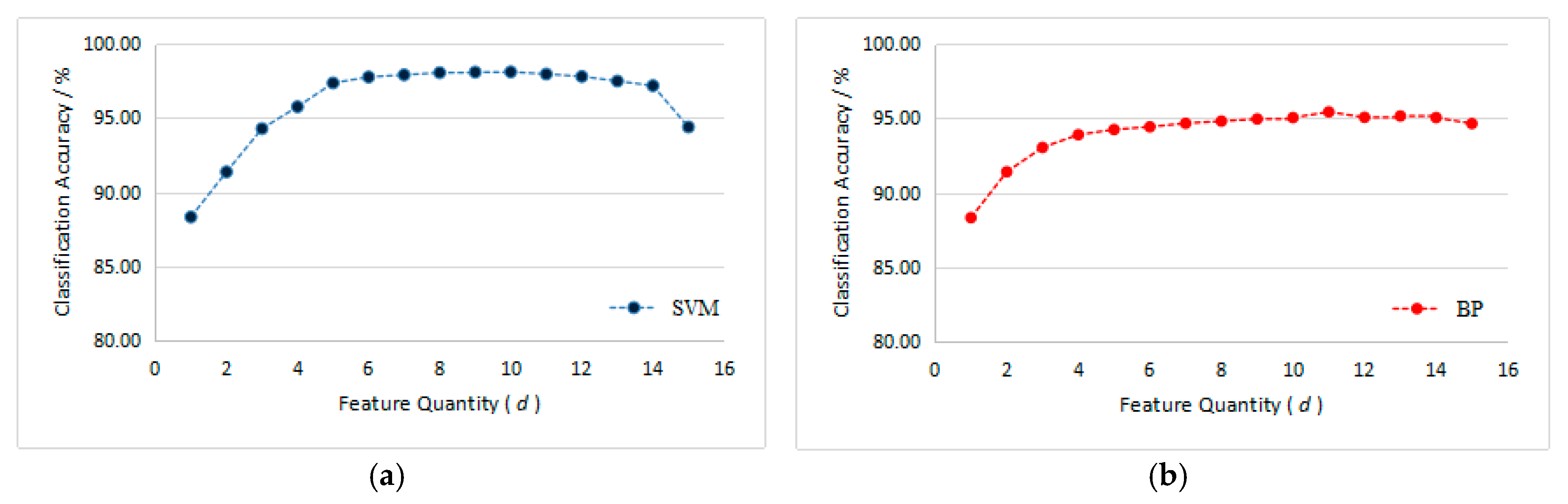
The classification accuracy of the features selected by SFFS are shown in Figure 4.
The SVM classifier improves significantly by adding features, until five features are applied and an accuracy of 97.36% is reached. After that, additional features cannot increase the accuracy by much, although the improvement continues. The best performance is reached when ten features are used, with a maximum classification accuracy of 98.11%. Then, adding features can only decrease the accuracy. When all fifteen features are used, the accuracy is 94.40%. One possible explanation for this phenomenon is that after ten features are used, the additional features do not provide more useful information for classification, and the irrelevant information, or even noise, complicate the problem. For the BP classifier, adding features cannot increase the accuracy as much as SVM. The accuracy is 94.25% when five features are used. After that, the accuracy increases slowly, with a maximum accuracy of 95.44% using eleven features. More details are shown in Table 4.
As can be seen from the first four rows of the table, when one feature or all fifteen features are employed, the accuracy of SVM and BP classifiers is close. The accuracy using all features is higher than using only one feature, which means that the process of high-power disk laser welding is complicated and cannot be monitoring through a single feature. From the fifth and sixth row of the table, it can be deduced that using the feature selection method, both SVM and BP reach a higher classification accuracy, but the improvement for the SVM classifier is much greater than BP. This may be caused by the instability of the BP method. Because the lack of effective initialization method, the BP training algorithm usually initializes randomly, and the initial values influence the classification ability of the BP classifier. The result is that even if the same feature subset is used, the classification accuracy of the BP classifier can be different. As the accuracy is chosen to evaluate the effectiveness of feature subsets in the SFFS algorithm, this feature selection method cannot effectively detect the optimal feature subset for the BP classifier. Consequently, compared to the other five methods, the SVM with feature selection method is more suitable for automatically monitoring the welding quality during high-power disk laser welding.
5. Conclusions
In order to recognize the welding quality automatically during high-power disk laser welding, the SVM method was employed to build the classifier. A feature selection method based on the SFFS algorithm was applied to detect the optimal feature subset for SVM. The SVM classifier generated by the ten selected features can reach an accuracy of 98.11% by 10-fold cross validation. Experiment results show that this method is satisfactory, and has the potential to be applied in the real-time monitoring of high-power laser welding.
The images of the metal vapor plume and spatters captured during high-power disk laser welding contain a lot of information associated with the welding quality. The fifteen extracted features, especially the centroid and height of the plume, the area, perimeter, centroid, average grayscale value and quantity of the spatters play very important roles in recognizing the welding quality.
Despite the many advantages of the proposed method, some limitations remain. The most essential one is that the testing phase of cross validation was not conducted during the welding, but using the data collected from the welding and simulating in computer. The computer used is a Lenovo ideapad 300-14IBR (CPU Intel Celeron N3150 1.60 GHz; RAM 8.00 GB). In MATLAB R2010b, the processing time, including image processing, feature extraction and classification, of 1 testing fold (550 samples) is 26.71 s for SVM and 24.92 s for BP, using the optimal feature subsets. However, many viable methods exist to reduce the processing time, such as using more advanced equipment and programming with C. Other than these, using the unsupervised mode for classification can be another solution. More experiments are in planning, and the aforementioned methods will be investigated.
Acknowledgments
This work was financially supported by the National Natural Science Foundation of China (51505158,11674106), and the Natural Science Foundation of Guangdong Province (2014A030310153). Many thanks are given to Katayama Laboratory of Joining and Welding Research Institute of Osaka University, for the technical assistance of laser welding experiments.
Author Contributions
Teng Wang, Juequan Chen and Xiangdong Gao conceived and designed the experiments; Juequan Chen and Xiangdong Gao performed the experiments; Teng Wang, Juequan Chen and Yuxin Qin analyzed the data; Teng Wang and Juequan Chen wrote the paper.
Conflicts of Interest
The authors declare that there is no conflict of interest regarding the publication of this paper.
References
- Altarazi, S.; Hijazi, L.; Kaiser, E. Process parameters optimization for multiple-inputs-multiple-outputs pulsed green laser welding via response surface methodology. In Proceedings of the 2016 IEEE International Conference on Industrial Engineering and Engineering Management (IEEM), Bali, Indonesia, 4–7 December 2016. [Google Scholar]
- You, D.Y.; Gao, X.D.; Katayama, S.J. Monitoring of high-power laser welding using high-speed photographing and image processing. Mech. Syst. Signal Process. 2014, 49, 39–52. [Google Scholar] [CrossRef]
- Cha, Y.J.; You, K.; Choi, W. Vision-based detection of loosened bolts using the Hough transform and support vector machines. Autom. Constr. 2016, 71, 181–188. [Google Scholar] [CrossRef]
- Cha, Y.J.; Choi, W.; Büyüköztürk, O. Deep Learning-Based Crack Damage Detection Using Convolutional Neural Networks. Comput-Aided Civ. Infrastruct. 2017, 32, 361–378. [Google Scholar] [CrossRef]
- Chen, J.G.; Wadhwa, N.; Cha, Y.J.; Durand, F.; Freeman, W.T.; Buyukozturk, O. Modal identification of simple structures with high-speed video using motion magnification. J. Sound Vib. 2015, 345, 58–71. [Google Scholar] [CrossRef]
- Cha, Y.J.; Chen, J.G.; Büyüköztürk, O. Output-only computer vision based damage detection using phase-based optical flow and unscented Kalman filters. Eng. Struct. 2017, 132, 300–313. [Google Scholar] [CrossRef]
- Cha, Y.J.; Wang, Z. Unsupervised novelty detection–based structural damage localization using a density peaks-based fast clustering algorithm. Struct. Health Monit. 2017. [Google Scholar] [CrossRef]
- Wang, E.J.; Lin, C.Y.; Su, T.S. Electricity monitoring system with fuzzy multi-objective linear programming integrated in carbon footprint labeling system for manufacturing decision making. J. Clean Prod. 2016, 112, 3935–3951. [Google Scholar] [CrossRef]
- Yin, S.; Luo, H.; Ding, S.X. Real-time implementation of fault-tolerant control systems with performance optimization. IEEE. Trans. Ind. Electron. 2014, 61, 2402–2411. [Google Scholar] [CrossRef]
- Wan, X.; Wang, Y.; Zhao, D.; Huang, YA.; Yin, Z. Weld quality monitoring research in small scale resistance spot welding by dynamic resistance and neural network. Measurement 2017, 99, 120–127. [Google Scholar] [CrossRef]
- Casalino, G.; Facchini, F.; Mortello, M.; Mummolo, G. ANN modelling to optimize manufacturing processes: The case of laser welding. IFAC-PapersOnLine 2016, 49, 378–383. [Google Scholar] [CrossRef]
- Vapnik, V.; Lerner, A. Pattern recognition using generalized portrait method. Autom. Rem. Control 1963, 24, 774–780. [Google Scholar]
- Vapnik, V.; Chervonenkis, A. A note on one class of perceptrons. Autom. Remote Control 1964, 25, 103. [Google Scholar]
- Liu, G.; Gao, X.D.; You, D.Y. Prediction of high power laser welding status based on PCA and SVM classification of multiple sensors. J. Intell. Manuf. 2016, 1–12. [Google Scholar] [CrossRef]
- Fan, J.; Jing, F.; Fang, Z.; Tan, M. Automatic recognition system of welding seam type based on SVM method. Int. J. Adv. Manuf. Technol. 2017, 92, 1–11. [Google Scholar] [CrossRef]
- Mekhalfa, F.; Nacereddine, N. Multiclass Classification of Weld Defects in Radiographic Images Based on Support Vector Machines. In Proceedings of the Tenth International Conference on Signal-Image Technology and Internet-Based Systems (SITIS), Marrakech, Morocco, 23–27 November 2014. [Google Scholar]
- Burges, C.J.C. A tutorial on support vector machines for pattern recognition. Data Min. Knowl. Discov. 1998, 2, 121–167. [Google Scholar] [CrossRef]
- Schölkopf, B.; Smola, A.J. Learning with Kernels: Support Vector Machines, Regularization, Optimization, and Beyond; MIT Press: Cambridge, MA, USA, 2002. [Google Scholar]
- Bennett, K.P.; Campbell, C. Support vector machines: Hype or hallelujah? ACM SIGKDD Explor. News. 2000, 2, 1–13. [Google Scholar] [CrossRef]
- Qiu, Z.Y.; Jin, J.; Lam, H.K.; Zhang, Y.; Wang, X.Y.; Cichocki, A. Improved SFFS method for channel selection in motor imagery based BCI. Neurocomputing 2016, 207, 519–527. [Google Scholar] [CrossRef]
- Tan, M.; Pu, J.; Zheng, B. Optimization of breast mass classification using sequential forward floating selection (SFFS) and a support vector machine (SVM) model. Int. J. Comput. Assist. Radiol. Surg. 2014, 9, 1005–1020. [Google Scholar] [CrossRef] [PubMed]
- Peng, H.; Fu, Y.; Liu, J.; Fang, X.; Jiang, C. Optimal gene subset selection using the modified SFFS algorithm for tumor classification. Neural Comput. Appl. 2013, 23, 1531–1538. [Google Scholar] [CrossRef]
- Pudil, P.; Novovičová, J.; Kittler, J. Floating search methods in feature selection. Pattern. Recognit. Lett. 1994, 15, 1119–1125. [Google Scholar] [CrossRef]
- Whitney, A.W. A direct method of nonparametric measurement selection. IEEE Trans. Comput. 1971, 100, 1100–1103. [Google Scholar] [CrossRef]
- Gonzalez, R.C.; Woods, R.E. Digital Image Processing, 3rd ed.; Pearson: London, UK, 2007. [Google Scholar]
- Gao, X.D.; Wen, Q.; Katayama, S.J. Analysis of high-power disk laser welding stability based on classification of plume and spatter characteristics. Trans. Nonferr. Met. Soc. China 2013, 23, 3748–3757. [Google Scholar] [CrossRef]
- Alpaydin, E. Introduction to Machine Learning; MIT Press: Cambridge, MA, USA, 2014. [Google Scholar]
- Rumelhart, D.E.; Hinton, G.E.; Williams, R.J. Learning representations by back-propagating errors. Nature 1986, 323, 533–536. [Google Scholar] [CrossRef]
Figure 1.
The flow chart of SFFS algorithm.

Figure 2.
Schematic diagrams of image processing: (a) original image; (b) grayscale image; (c) binary image of plume; (d) binary image of spatters.
Figure 2.
Schematic diagrams of image processing: (a) original image; (b) grayscale image; (c) binary image of plume; (d) binary image of spatters.

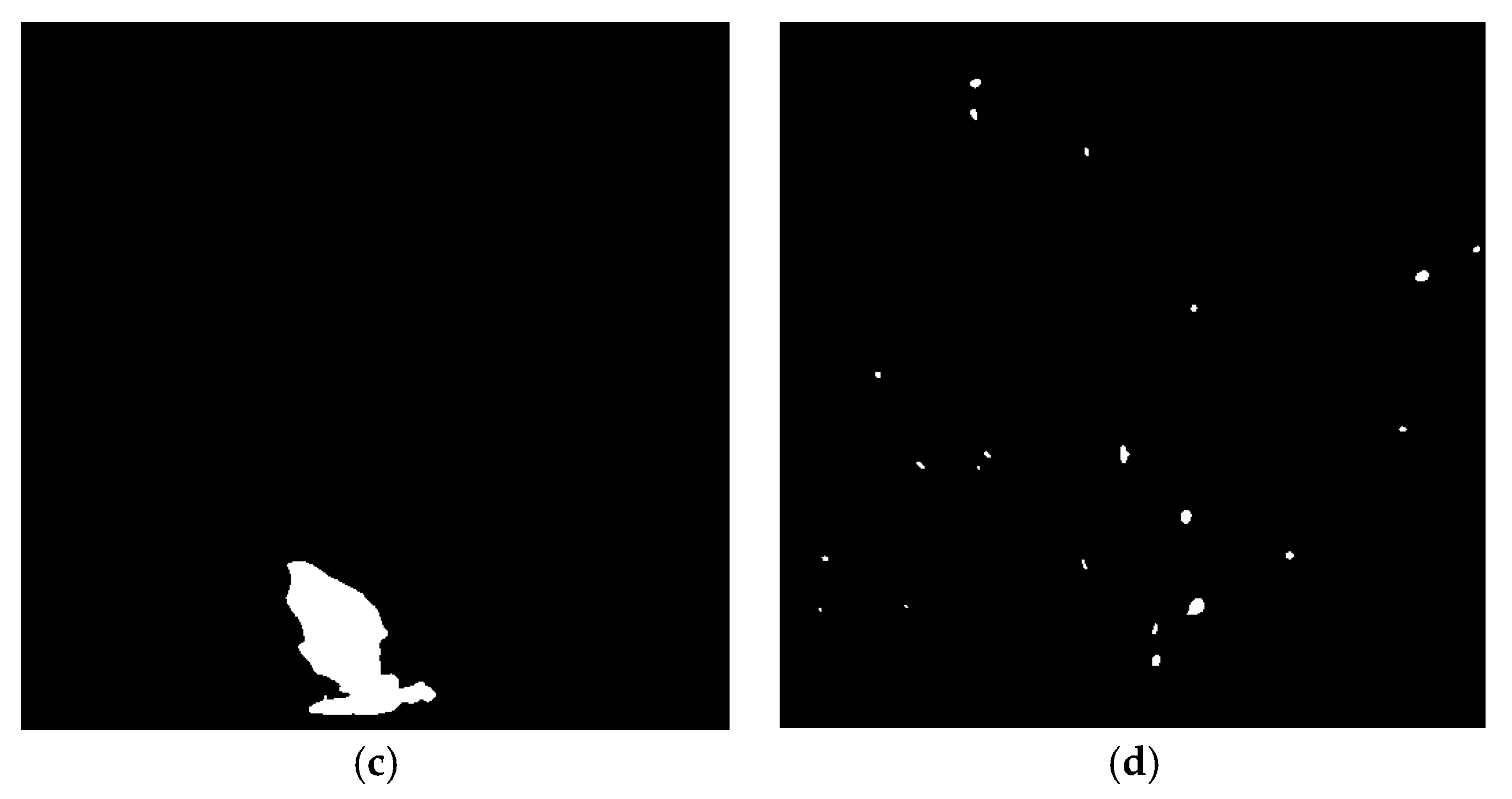
Figure 3.
Welded seams of different welding speeds: (a) 3 m/min; (b) 4.5 m/min; (c) 6 m/min.
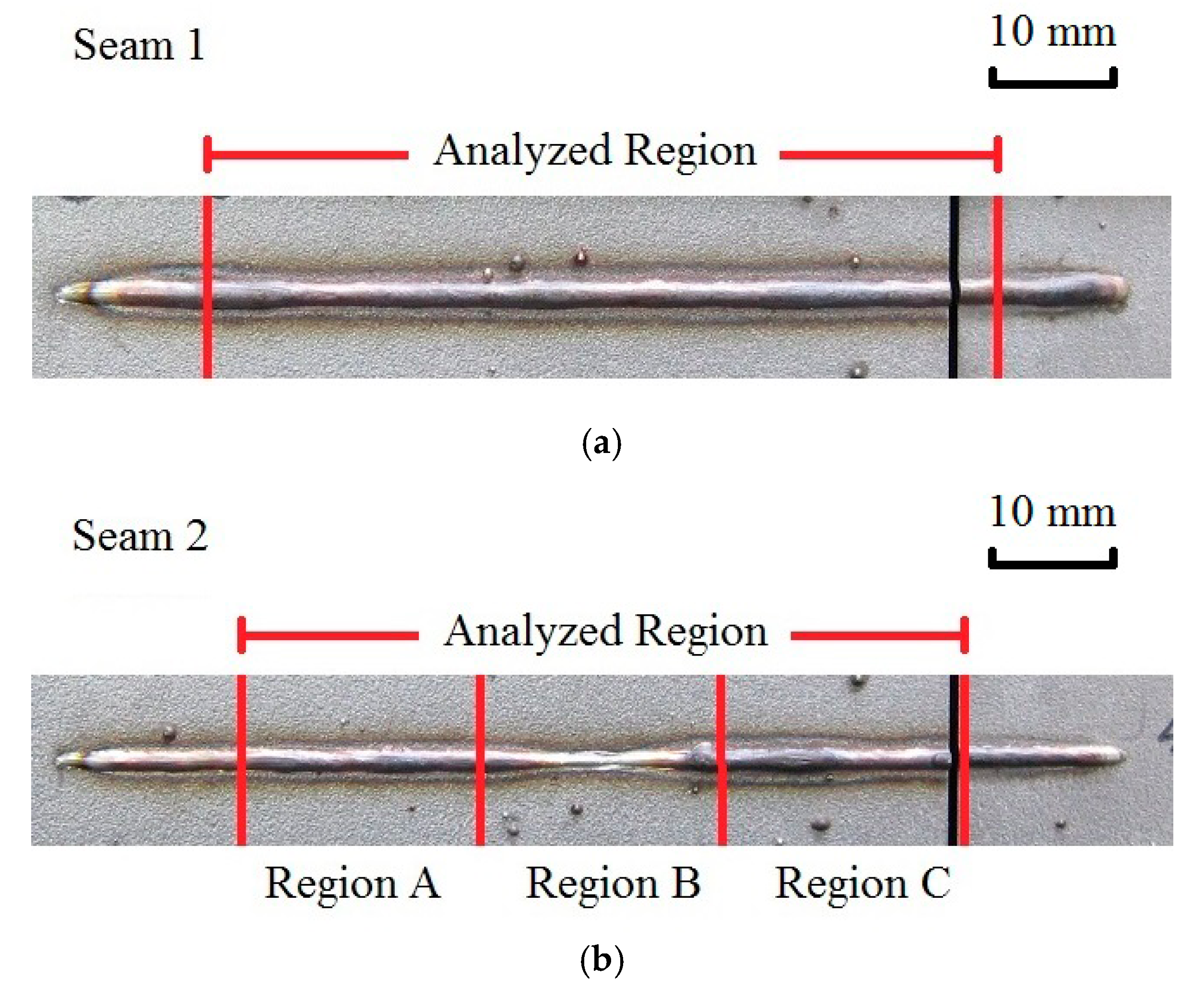

Figure 4.
The classification accuracy of different classifiers using the selected features: (a) SVM classifier; (b) BP classifier.
Figure 4.
The classification accuracy of different classifiers using the selected features: (a) SVM classifier; (b) BP classifier.

Table 1.
Details of different welding speeds.
| Welding Speeds (m/min) | Weld Length (mm) | Time (s) | Captured Images (Frame) |
|---|---|---|---|
| 3 | 90 | 1.8 | 3600 |
| 4.5 | 90 | 1.2 | 2400 |
| 6 | 90 | 0.9 | 1800 |
Table 2.
Fifteen extracted features.
| No. | 1 | 2 | 3 | 4 | 5 | 6 | 7 | |
| Feature | Ap | Pp | Cp(i) | Cp(j) | Hp | Wp | Gp | |
| No. | 8 | 9 | 10 | 11 | 12 | 13 | 14 | 15 |
| Feature | As | Ps | Cs(i) | Cs(j) | Gs | Qs(a) | Qs(l) | Qs(r) |
Table 3.
The classification accuracy of each feature.
| No. of Feature | Accuracy (SVM) (%) | Accuracy (BP) (%) | ||||
|---|---|---|---|---|---|---|
| Overall | Class R | Class E | Overall | Class R | Class E | |
| 1 | 66.09 | 95.43 | 14.75 | 66.09 | 94.14 | 17.00 |
| 2 | 68.04 | 93.51 | 23.45 | 67.98 | 91.49 | 26.85 |
| 3 | 84.44 | 95.74 | 64.65 | 84.56 | 94.63 | 66.95 |
| 4 | 81.18 | 86.20 | 72.40 | 81.33 | 86.49 | 72.30 |
| 5 | 81.25 | 93.43 | 59.95 | 80.98 | 90.89 | 63.65 |
| 6 | 75.29 | 84.09 | 59.90 | 75.60 | 83.23 | 62.25 |
| 7 | 63.64 | 100.00 | 0.00 | 63.64 | 100.00 | 0.00 |
| 8 | 88.22 | 98.11 | 70.90 | 88.31 | 97.66 | 71.95 |
| 9 | 85.24 | 94.91 | 68.30 | 85.16 | 94.71 | 68.45 |
| 10 | 87.84 | 94.51 | 76.15 | 87.76 | 94.54 | 75.90 |
| 11 | 86.53 | 91.00 | 78.70 | 86.44 | 91.29 | 77.95 |
| 12 | 88.35 | 95.63 | 75.60 | 88.35 | 95.54 | 75.75 |
| 13 | 74.95 | 79.46 | 67.05 | 74.93 | 80.69 | 64.85 |
| 14 | 82.69 | 90.51 | 69.00 | 82.69 | 90.51 | 69.00 |
| 15 | 85.49 | 93.57 | 71.35 | 85.44 | 92.57 | 72.95 |
Table 4.
The performance of different methods.
| ID | Method | d | Accuracy (%) | Features | ||
|---|---|---|---|---|---|---|
| Overall | Class R | Class E | ||||
| 1 | BP | 1 | 88.38 | 95.51 | 75.90 | 12 |
| 2 | SVM | 1 | 88.35 | 95.63 | 75.60 | 12 |
| 3 | BP | 15 | 94.89 | 98.51 | 88.55 | All |
| 4 | SVM | 15 | 94.40 | 99.57 | 85.35 | All |
| 5 | BP | 11 | 95.40 | 98.66 | 89.70 | 2,4,6,8,9,10,11,12,13,14,15 |
| 6 | SVM | 10 | 98.11 | 99.43 | 95.80 | 3,4,5,8,9,10,11,12,14,15 |
© 2017 by the authors. Licensee MDPI, Basel, Switzerland. This article is an open access article distributed under the terms and conditions of the Creative Commons Attribution (CC BY) license (http://creativecommons.org/licenses/by/4.0/).
Share and Cite
MDPI and ACS Style
Wang, T.; Chen, J.; Gao, X.; Qin, Y. Real-time Monitoring for Disk Laser Welding Based on Feature Selection and SVM. Appl. Sci. 2017, 7, 884. https://doi.org/10.3390/app7090884
AMA Style
Wang T, Chen J, Gao X, Qin Y. Real-time Monitoring for Disk Laser Welding Based on Feature Selection and SVM. Applied Sciences. 2017; 7(9):884. https://doi.org/10.3390/app7090884
Chicago/Turabian StyleWang, Teng, Juequan Chen, Xiangdong Gao, and Yuxin Qin. 2017. "Real-time Monitoring for Disk Laser Welding Based on Feature Selection and SVM" Applied Sciences 7, no. 9: 884. https://doi.org/10.3390/app7090884
Note that from the first issue of 2016, this journal uses article numbers instead of page numbers. See further details here.