Article

Road Safety Risk Evaluation Using GIS-Based Data Envelopment Analysis—Artificial Neural Networks Approach

1
Transportation Research Institute (IMOB), Hasselt University, Diepenbeek 3590, Belgium
2
Taxila Institute of Transportation Engineering, Department of Civil Engineering, University of Engineering & Technology, Taxila 47050, Pakistan
3
School of Transportation, Southeast University, Nanjing 210096, China
4
Faculty of Engineering Technology, Hasselt University, Diepenbeek 3590, Belgium
*
Author to whom correspondence should be addressed.
Appl. Sci. 2017, 7(9), 886; https://doi.org/10.3390/app7090886
Submission received: 31 July 2017 / Revised: 20 August 2017 / Accepted: 22 August 2017 / Published: 29 August 2017
(This article belongs to the Special Issue Application of Artificial Neural Networks in Geoinformatics)

Abstract

:
Identification of the most significant factors for evaluating road risk level is an important question in road safety research, predominantly for decision-making processes. However, model selection for this specific purpose is the most relevant focus in current research. In this paper, we proposed a new methodological approach for road safety risk evaluation, which is a two-stage framework consisting of data envelopment analysis (DEA) in combination with artificial neural networks (ANNs). In the first phase, the risk level of the road segments under study was calculated by applying DEA, and high-risk segments were identified. Then, the ANNs technique was adopted in the second phase, which appears to be a valuable analytical tool for risk prediction. The practical application of DEA-ANN approach within the Geographical Information System (GIS) environment will be an efficient approach for road safety risk analysis.

1. Introduction

Crash injury severity has always been a major concern in highway safety research. To model the relationship between crash occurrence along with severity outcomes, related traffic features, and contributing factors, a large number of advanced models have been proposed. Road safety research incorporates a broad exhibit of research territories, and the most successful of them is crash information investigation. There have been a lot of discussion about crash information-based safety analysis and other distinguishable activity attributes have been proposed, more regularly than crashes, as an option. In any case, investigation of crash information remains the most broadly received way to deal with the safety of a transportation system (e.g., expressways, arterials, crossing points, etc.). The traditional approach is to build up connections between crash recurrence, traffic flow attributes, and geometry of the roads [1]. On the one hand, the impact of the geometric design on the probability of a driver behavior has been very much archived in conventional safety studies. This course of research is useful in settling on choices in such things as installing cautioning signs on roadway areas, etc. On the other hand, Average Annual Daily Traffic (AADT) is a generally used indicator for measuring the traffic movement conditions, as it is recorded by most organizations around the nation/the world, is accessible to all roadway areas, and gives a measure of introduction to the specific roadway segment. Crash recurrence examination in view of AADT is a total or aggregate approach to take a glance at the crash information where the recurrence of crashes is computed, by amassing the crash information over particular eras (months or years) and areas (particular roadway segments) [2].
During road safety analysis of a road, a major target is to locate those segments which are dangerous, and then to identify the factors influencing its safety level. This study focuses on the concept that crashes can be decreased by better assessment of road hazard incremental elements, and by recognizable proof of hazardous segments at the initial stage, and after that, assessment of very dangerous sections with reference to the major contributing components is conducted in the second stage. In doing so, a combination of Data Envelopment Analysis (DEA) with Artificial Neural Networks (ANNs) is applied to evaluate the performance of roads with reference to safety conditions. The outcome is able to help decision makers/safety engineers to build a valuable system to analyze risk and significant attributes. Although it is new in the road safety research field, such an integrated mechanism has been popular in other sectors like banks, hospitals, schools, and corporations. Some researchers have used a combination of DEA-ANNs to evaluate performance (efficiency/risk) of rail transport, power suppliers, etc. [3,4,5]. DEA-ANNs was also used for efficiency classification by different researchers for banks and corporate companies [5,6,7]. For analysis regarding hospitals and large companies, screening of training data was also evaluated by using the DEA-ANNs technique. In addition, DEA-ANNs was also introduced for data processing [8,9,10,11,12,13], and will be more useful when applied within a Geographical Information System (GIS) environment. In this study, this integrated concept, which is popular in other sectors, is introduced to evaluate the safety performance (risk evaluation) of motorways. This evaluation of risk helps decision makers to decide on economical investment for risky segments, along with related factors, and consequently to reduce the cost of risk evaluation.

2. Literature Review

2.1. Risk and Road Safety Analysis

Usually, road safety performance is evaluated on the basis of ‘Risk’ which is associated with the number of crashes and casualties, known as the road safety outcome. In the field of road safety, the risk is defined as ‘the road safety outcome to the amount of exposure’ as shown in Equation (1):
R i s k   =   R o a d   S a f e t y   O u t c o m e E x p o s u r e
Exposure can be measured using different parameters; while comparing the performance of road segments, it can be measured as vehicle miles traveled, vehicle hours traveled, volume and number of trips, etc., however for countries it can be passenger kilometers travelled, population and number of registered vehicles, etc. [14,15]. Risk assessment is necessary for road safety performance analysis. Although risk can be analyzed on the basis of direct calculation using outcome by exposure, in the case of multiple outcomes and multiple input, it is difficult to deal with the calculation. Crashes are random events, and their outcome can also vary, as in one crash there may be zero fatalities, or fifty or more fatalities. Thus, a method that can deal with multiple outputs can be beneficial in calculating risk for road safety performance analysis of different units.

2.2. DEA for Road Safety Analysis

Road safety performance analysis of highways is an important task for the safety of travelers. To analyze the safety performance of certain attributes, a benchmarking mechanism has remained a basic procedure to be adopted by researchers [16,17,18]. With reference to the applied techniques for this purpose, DEA has been a popular technique with its theoretical basis in linear programming. Evolving the concept of DEA from research work in 1978, Charnes et al. [19] applied a linear program to estimate an empirical production technology frontier (bench marking) for the first time [19]. In the basic DEA model, the definition of the best practices relies on the assumption that inputs have to be minimized and outputs have to be maximized (such as in the economics field). However, to use DEA for road safety risk evaluation, the target becomes the output, i.e., the number of traffic crashes, to be as low as possible with respect to the level of exposure to risk. Therefore, the DEA frontier based Decision Making Units(DMUs) or the best-performing road segments are those with minimum output levels given the input levels, and other segments’ risk is then measured relative to this frontier [20].
Mathematically, to use DEA for road safety evaluation, the model is shown as follows:
min R 0 = r = 1 s u r y r 0 s . t . i = 1 m v i x i 0 = 1 , i = 1 m v i x i j r = 1 s u r y r j 0 , j = 1 , , n u r , v i 0 , r = 1 , , s , i = 1 , , m
where yrj and xij are the rth output and ith input respectively of the jth DMU, ur is the weight given to output r, and vi is the weight given to input i.
In view of the model applications for road safety analysis, road safety condition was compared to 21 European countries [16] and an ideal trauma management record score was also calculated by using DEA [21]. Furthermore, using population, passenger-kilometers, and passenger cars as inputs, and the number of fatalities as output, DEA was used for the evaluation of risk level of countries [22]. Monitoring of yearly progress in road safety was also conducted by utilizing the DEA technique [23]. Adding to road safety determination on a national level for 27 Brazilian states, two fundamental indicators accessible in Brazil: death rate (fatalities per capita) and casualty rate (fatalities per vehicle and fatalities per vehicle kilometer traveled) were focused upon [24]. From the literature review on DEA application in the field of road safety, it was confirmed that DEA is one of the established techniques to evaluate the risk level of road safety.

2.3. ANNs for Road Safety Analysis

Artificial Neural Networks is a model instrument of nonlinear statistical data that can be used to model a complex relationship between input and output to seek patterns. ANNs has been often implemented in many fields of science for prediction [25]. In road safety research, ANNs was applied to investigate crashes with reference to driver, vehicle, roadway, and condition attributes [26]. After application of ANNs, the impact of factors like seatbelt usage, light condition, and driver’s liquor utilization on driver’s safety was evaluated [27]. ANNs was also applied to determine the relationship between crash severity and the model parameters including years, highway sections, section length (km), AADT, the degree of horizontal curvature, the degree of vertical curvature, heavy vehicles (percentage), and season summer (percentage). The results shown that degree of vertical curvature has strong impact on number of crashes [28]. By modeling AADT, SL (Posted speed limit), Gradient (Average segment gradient), and Curvature (Average segment curvature) against road crashes, it was concluded that ANN was superior to multivariate Poisson-lognormal models [29]. From the literature review, we can summarize that ANNs was previously used as a crash data analysis model, which was a useful technique to study road-related features, geometry, and other contributing factors to road safety.

2.4. DEA-ANNs Approach

The combination of DEA and ANNs has not been applied in the road safety field, but it is popular in other fields like banks and corporate sectors. From the previous studies it was concluded that DEA is powerful for efficiency calculation, but for prediction purposes ANNs is ahead, so a discussion started after [30] on combining these two techniques to obtain the best possible outputs, i.e., efficiency calculation for ranking and prioritizing and then efficiency prediction for factor analysis purpose. To validate this combination, efficiency prediction was performed for 50 companies [31], 19 power plants [32], 49 Indian business schools [5], 102 bank branches [7], and 45 countries [33]. Efficiency classification was also tested by studying 142 bank branches [34] and 23 supplier companies [35]. Following the similar pattern, the DEA-ANNs approach is selected in this study for road safety risk evaluation and analysis of factors affecting risk.

2.5. GIS for Road Safety Analysis

“While geometrical concept can be enriched by culture-specific devices like maps, or the terms of a natural language, underneath this variability lies a shared set of geometrical concepts. These concepts allow adults and children with no formal education, and minimal spatial language, to categorize geometrical forms and to use geometrical relationships to represent the surrounding spatial layout.” (Elizabeth S. Spelke-Harvard). GIS has gained a reputation that provides a better visualization of a large data set for understanding and decision making processes. GIS-provided maps which helped in identifying the crash concentration areas, located along the major road in the main urban areas [36]. During the road safety analysis of motorway (M-25), GIS provided relevant data on road accidents, traffic and road characteristics for 70 segments [37]. High risky sections on the basis of potential crash cost for expressways of Shanghai with the application of GIS has been clearly mapped [38]. Zonal crash frequency has also been expressed through GIS, showing association with several social-economic, demographic, and transportation system factors [39]. Through spatial analysis of high risk areas, pedestrian crashes have also been mapped in Tehran [40]. In Belgium, through the use of GIS and point pattern techniques, mapping road-accident black zones has been conducted within urban agglomerations [41]. GIS has also been used to explore the spatial variations in relationship between Number of Crashes and other explanatory variables of 2200 Traffic Analysis Zones (TAZs) in the study area, Flanders, Belgium [42,43]. GIS was used for modelling crash data at a small-scale level in Belgium, which permitted the identification of several areas with exceptionally high crash data. It endorsed more effective reallocation of resources and more efficient road safety management in Belgium [44].

2.6 ANN-GIS Approach

ANNs has been introduced as a mapping tool to GIS to perform a predictive capability for joint operations [45]. Although GIS in combination with ANNs was popular in the fields of geoscience, irrigation, meteorology and Agriculture, it has been tested in the field of road safety by applying deep learning models using a Recurrent Neural Network (RNN) to predict the injury severity of traffic crashes for the North-South Expressway-Malaysia [46]. Previously this technique had been applied for sediment prediction in Gothenburg harbor [45], landslide susceptibility using the landslide occurrence factors produced with the help of a ANNs model [47], detection of flood hazards in the Blue Nile, White Nile, Main Nile, and River Atbara [48], macrobenthos habitat potential mapping regarding Macrophthalmus dilatatus, Cerithideopsilla cingulata, and Armandia lanceolate [49], learning the patterns of development in the region [50], tunneling performance prediction required in routine tunnel design works and performance in terms of stability as well as impact on surrounding environment [51], and deforestation maps production to determine the relationship between deforestation and various spatial variables such as the vicinity to roads and to expenditures, forest disintegration, elevation, slope, and soil type [52].

2.7. Research Gap

DEA is popular as an optimization tool with its theoretical background in linear programming. DEA is popular with reference to benchmarking mechanism for efficiency and risk evaluation [3,6]. Previously, DEA was popular with its multi stage properties, but it has shortcomings with respect to its prediction capabilities, which reduces its application. A powerful technique, ANN, has been joined with DEA to fill that gap. Finally, with the predictive potential of ANNs and the optimization capacity of DEA performing complementary features, a prominent modeling option is envisioned [3,6]. The performance of the DEA-ANNs technique in the field of road safety for decision making mechanisms for road safety performance analysis was evaluated. This is the first study for an application of the DEA-ANN approach within a GIS environment for road safety performance analysis, using a case study on Motorways. This will lead traffic engineers and decision makers to better visualize the risky sections and key factors for road safety condition improvement.

3. Materials and Methods

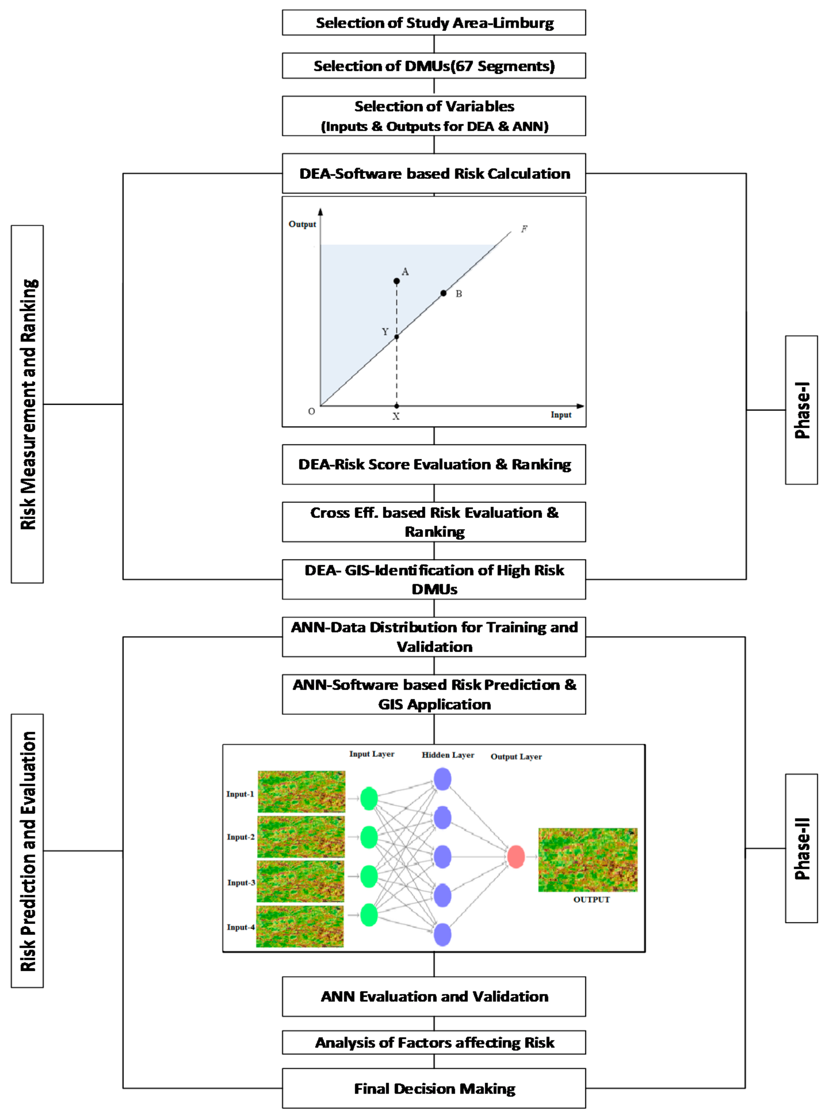
3.1. Basic Framework of the Analysis

Road authorities have to prioritize the sites which require safety treatment, due to budget limitations. So in this study, a two phase framework was proposed for road safety risk evaluation, as shown in Figure 1. In the first phase, the number of crashes and fatalities was evaluated against exposure variables, with the help of DEA to calculate the risk level of road segments. In the second phase, that risk was predicted and evaluated with the help of ANNs.

3.2. Data Description and Selection of Variables

The study area selected for this study was two motorways in Belgium named E-313 and E-314 (Limburg Province Sections with a total length of 103 km). Each Motorway has segments, traffic-related characteristics, and road network segmentation derived from the FEATHERS model [53]. In this study, a segment with at least one crash was considered as a decision-making unit (DMU) to analyze the road safety condition. According to this criterion, 67 segments are selected for these two motorways. The crash data used in this study consisted of a geographically coded set of crash data that occurred between 2010 and 2012, which was provided by the Flemish Ministry of Mobility and Public Works, as shown in Table 1. The first and very critical step in conducting an analysis is the selection of inputs and outputs variables. For this purpose in the first stage (DEA), those variables which were the exposure variables and could not be directly affected by a traffic engineer/decision maker were selected to calculate risk, while in the second stage (ANN) those variables (i.e., Horz and Vert Curve design, speed, and flow) which could be altered or improved by directly changing certain parameters, were selected. So, the target while calculating risk was to reduce the number of crashes (NoC) and casualties (NoAP) with the increase of average volume to capacity on each segment (V/C), total daily vehicle miles travelled on each segment (VMT) and total daily vehicle hours travelled on each segment (VHT). A traffic engineer cannot directly change V/C, VMT, or VHT; however, the geometric design (Horz and Vert Curve), speed (speed limit) and flow (by controlling access) so practically, a selection of variables was targeted according to the feasibility of the problem's solution. To confirm the validity of the DEA model condition, an isotonicity test [54] was conducted. An isotonicity test comprises the intention of all inter-correlations between inputs and outputs for detecting whether increasing amounts of inputs lead to greater outputs. As positive correlations were established, the isotonicity test was accepted and the presence of the inputs and outputs was reasonable. However there are no diagnostic checks for improper model specification detection in DEA [55]. However, a general rule of thumb, the minimum number of DMUs is higher than three times the number of inputs plus outputs [56]. In our study with a total of three inputs and two outputs, so a set of 15 data points would be optimal; we have 67 data segments.

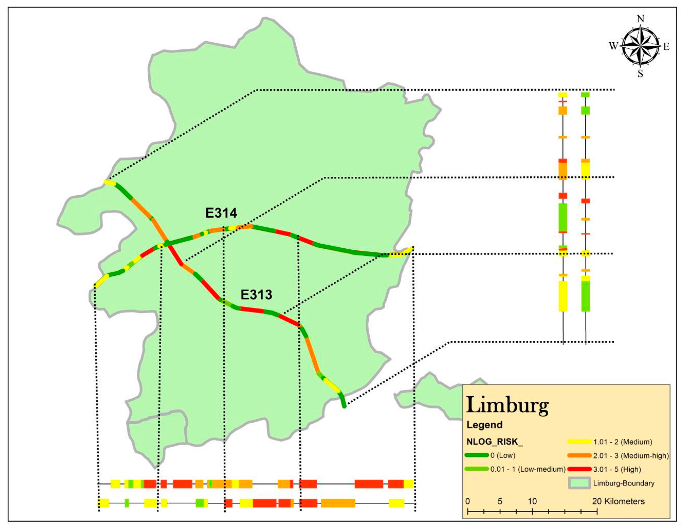
3.3. Phase-I: Application of DEA for Risk Calculation and Ranking

As there were two major phases of modeling, we had decide on the variables for both phases. The initial target was to evaluate risk with reference to the variables that were basically exposure variables. In the basic DEA model, the definition of the best practice relied on the assumption that inputs had to be minimized, and outputs have to be maximized (such as in the economics field). However, to use DEA for road safety risk evaluation, the target became the output, i.e., the number of traffic crashes, to be as low as possible with respect to the level of exposure to risk.
There are two basic concepts in application of DEA, starting from efficiency as in Equation (3), and converting into calculation of risk as shown in Equation (4).
Efficiency: The basic concept of DEA-Efficiency calculation is as follows:
E f f i c i e n c y   =   W e i g h t e d   S u m   o f   O u t p u t W e i g h t e d   S u m   o f   I n p u t   =   M a x i m i z e   O u t p u t M i n i m i z e   I n p u t
Risk: The basic concept of DEA-Risk calculation in connection between Equations (1) and (3):
R i s k   =   W e i g h t e d   S u m   o f   O u t p u t W e i g h t e d   S u m   o f   I n p u t   =   M i n i m i z e   O u t p u t M a x i m i z e   I n p u t   =   R o a d   S a f e t y   O u t c o m e E x p o s u r e
So the equation to calculate the Risk value through DEA is as follows:
R i s k   =   U 2 ( N o C ) + U 1   ( N o A P ) V 1   ( V / C ) + V 2   ( V M T ) + V 3   ( V H T )
where U1 = weights for 1st output (NoC), U2 = weights for 2nd output (NoAP); V1 = Weights for 1st Input (V/C), V2 = weights for 2nd Input (VMT), V3 = weights for 3rd Input (VHT).
After calculation of Risk value, for ranking purposes, a cross-efficiency approach was one of the best methods to calculate A cross-risk value for ranking purposes. DEA has an attractive feature in that each DMU can have its own input and output weights, which leads to difficulty in making a comparison between DMUs. To compare DMUs, a Cross efficiency matrix (CEM) was developed as a DEA extension tool to assist in identifying the overall best or worst performer among all DMUs and rank them. Its basic idea is to apply DEA in a peer assessment instead of a self-assessment mode. Specifically, the CEM calculates the performance of a DMU with a concept by using not only its own optimal input and output weights, but also those of all other DMUs. Results can then be accumulated in a CEM as shown in Table 2. In the CEM, the element in the ith row and jth column signifies the risk scores of DMU j using the optimal weights of DMU i. The basic DEA risk is thus positioned in the principal diagonal. The average of each column of the CEM is calculated as a mean cross risk value for each DMU [20]. Since the same weighting process is applied for all the DMUs, their evaluations can then be made on a comparison basis, with a higher cross-risk score indicating a higher risky DMU.
For those DMUS, which have illogical weights in the basic DEA model, a relatively low or higher risk value will be calculated. Therefore, for ranking purpose, this method serves a type of sensitivity analysis by applying a method of a different set of weights to each DMU, with a back channel mechanism of self-generated weights rather than an externally imposed [20]. So the target value, which is a value of 1 to be considered for the best DMU, can now be changed, and after application of CEM it can vary, but the selection of best DMU (with the lowest Risk) will be easier.So after applying model (1) for calculating risk R0 in road safety field, the lowest level has been considered as the frontier of safety. As explained above, for ranking purposes, a cross risk procedure [20] has been adopted to obtain the best ranking, as shown in Table 3.
The major advantage of using DEA here is that it can handle multiple inputs and multiple outputs. Moreover, DEA has some benefits as it does not require an assumption of a functional form relating inputs to outputs; DMUs considered in DEA are directly compared against a peer or combination of peers; Inputs and outputs used in DEA can have different measurement units. In this study, number of crashes (NoC) and number of affected persons-injured or killed (NoAP) are considered as two outputs, while exposure variables—average volume to capacity on each segment (V/C), total daily vehicle miles travelled on each segment (VMT), and total daily vehicle hours travelled on each segment (VHT)were considered as three inputs. Although the segment length also varied, it was not included here because it was already been involved in the backup calculation of VMT.
Based on Model (1), the range of risk value began at 1 and proceeded to a higher value, so a segment with a value of 1 was considered safest, while the road segment with the highest value was considered the most dangerous. Moreover, the cross risk method [20] was used to make all the DMUs comparable. Table 3 presents the results. As the ranking was done on a priority basis to evaluate the safety condition of that segment, the risk value of 91.07 was the highest value in the table and was ranked first (i.e., the most risky segment). The top 10 riskiest segments are shown in Table 3 to explain an idea of risky segment selection for improvement.
Furthermore, risk value was normalized by applying natural log, and with the help of GIS, a complete spatial map of both motorways is shown in Figure 2. A straight line demonstration provides an insight in locating the most riskiest segment on a motorway or highway.

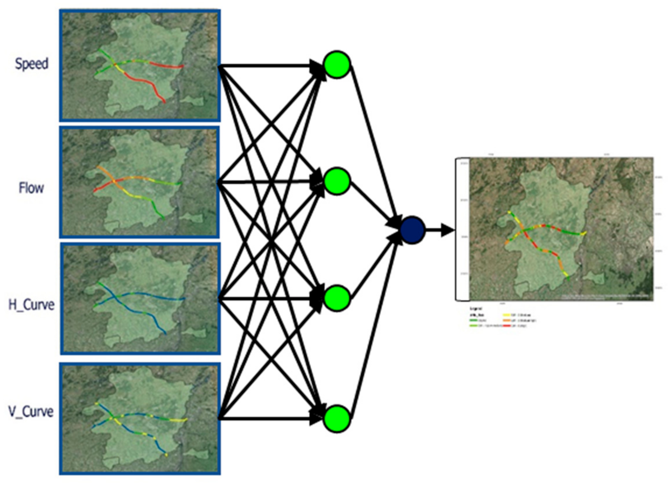
3.4. Phase-II: Application of ANNs Model for Risk Prediction and Evaluation

In the second phase, the dependent variable is the risk value generated by the DEA model, was transformed by applying natural log to have data normalized. For independent variables, speed could be controlled by controlling the speed limit; flow was directly related to the number of vehicles, and could be controlled by controlling access; horizontal curve could be removed or altered as per infrastructural changes, and the same was the case for vertical curve as a geometric design feature. So for the application of ANN, data was distributed on the basis of a K-Fold mechanism with five folds (i.e., distribution is as 53 segments-DMUs for Training and 14 segments-DMUs for validation).
ANNs, unlike other modeling platforms, requires some form of model validation to aid in the model-building process and to help prevent overfitting of the model. The basic idea behind validation (or cross-validation) is to hold a subset of the data out of the model-building process. This process forms two partitions of the data, a training set and a validation set (note that a third set, or test set, can also be used). The model is built using the training set, while the k-fold validation set is then used to assess how well the model performs, and to aid in model selection. The most mainstream decision for the quantity of concealed layers is used. A solitary concealed layer is typically adequate to catch even extremely complex connections between the indicators. The quantity of links in the shrouded layers likewise decides the level of multifaceted nature of the connection between the indicators that the system catches [57].
From one viewpoint, utilizing an excessive couple of links is not adequate to catch complex connections (e.g., review the unique instances of a straight relationship in direct and calculated relapse, in the extraordinary instance of zero links or no shrouded layer). Then again, an excessive number of links may prompt overfitting. A dependable guideline is, to begin with (number of indicators) links and reduce or increment gradually while checking for overfitting. Another approach is to start with the default neural model, with one layer and four nodes, and then run a much more complex model with two layers and several nodes, and different activation functions. If the fit statistics do not improve substantially with a more complex model, then a simpler model may suffice [57]. We applied a simpler model to check the performance of the ANNs model in our case of risk evaluation, as shown in Figure 3. After running the model as shown in Figure 3, we displayed the model structure. We saw input variables mapping to each of the activation functions in the hidden layer, and nodes in the hidden layer mapping to the output layer. The background mechanism in each of the nodes in the hidden layer designated that the Gaussian activation function was used. Model results for both the training and validation sets are shown in Table 4. The response variable (risk) for this model was continuous. Like other techniques, it was necessary to follow the validation mechanism. With the validation mechanism and separation of the data into two sets, unbiased results were provided.
In this study, as discussed earlier, original data were distributed into two parts. Out of 67 segments, 53 as the major data set were used for the training of the ANNs setup, while the remaining 14 were used for validation after model building. The training set was the part that estimated model parameters. The validation set was the part that assessed or validated the predictive ability of the model. In addition, the most critical validation was applied in this study. Specifically, the K-Fold technique was adopted, which divided the original data into K subsets. In turn, each of the K sets is used to validate the model fit on to the rest of the data, fitting a total of K models. The model giving the best validation statistic was chosen as the final model. This method was best for small data sets because it made efficient use of limited amounts of data [57,58].The ANN based predicted value of risk was mapped in the GIS environment as shown in Figure 4, showing a red line as the riskiest segments, while dark green segments are the safest as there zero crashes on these segments.
The values of R-square and Root Mean Square Error (RMSE) are the two basic validation indicators for testing the goodness-of-fit of the model. ANNs is a very flexible model and has a tendency to overfit data. When that happens, the model predicts the fitted data very well, but predicts future observations poorly. To mitigate overfitting, the neural platform applies a penalty on the model parameters and uses an independent dataset to assess the predictive power of the model. The applied technique to control overfitting is the squared method. This method is applied if it is considered that independent variables are contributing to the predictive ability of the model.
During the analysis, the graphical representation of data showed a better performance both in the case of training and validation data. The data distribution was adopted in five segments, having a distribution of 53 segments for training and 14 segments for validation. The plots showing the perfection of predictability were shown in Figure 5 for both training and validation data. The values of R-square were also almost similar for both major and training and validation data sets.
The contribution of factors associated with risk can be analyzed by the importance of the variables (i.e., Flow, Speed, Vertical and Horizontal Curve).The impact of variables is one of the necessary targets to analyze and improve the safety performance of the roads. Traffic safety engineers always search for the relationships between factors and safety performance indicators (i.e., Risk). The relationship can be observed in Table 5, which shows that speed and flow were two major factors which are having a high impact on risk.
A comprehensive analysis to overview the importance of factors provides traffic engineers to take a decision during road safety analysis and implementation procedure.

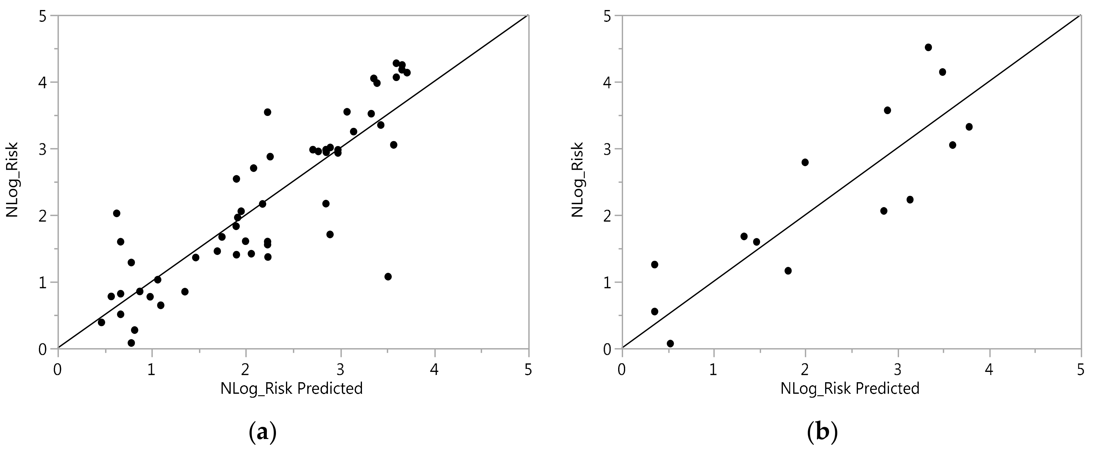
3.5. Model Selection Criteria

In order to assess the performance of the DEA-based Risk prediction models, a number of evaluation criteria were used to evaluate these models. These criteria were applied to measure how close the real values were to the values predicted using the developed models. They included Root Mean Square Error (RMSE) and the correlation coefficient R or R2. These are given in Equations (6) and (7) respectively [59].
R M S E   =   1 n i   =   1 n ( y i y ^ i ) 2
R   =     i   =   1 n   ( y i y ¯ )   ( y ^ i y ^ ¯ ) i   =   1 n   ( y i y ¯ ) 2   i   =   1 n   ( y ^ i y ^ ¯ ) 2  
where y is actual Risk values, y ^ is the estimated Risk values using the proposed techniques, and n is the total number of observations of DMUs.

4. Results

In order to find the factors influencing the road safety risk, ANNs and multiple linear regression (MLR) were generated using the Road Traffic and Crash data obtained for European routes (E-313&E-314) of Limburg (Belgium). Although the basic target was to implement the ANNs model, regression analysis was also conducted to assess the performance of ANNs.

4.1. Performance of Model

The main objective of the methods (ANNs and MLR) was to fit an accurate model for risk prediction. The adequacy of such models are typically measured either by the coefficient of determination of the predictions against actual values (R2) or by RMSE. Figure 6 shows the comparative diagram of prediction between ANNs and MLR.
The graph shown in Figure 6 suggests that ANNs is a better predictor than MLR. Moreover, if we considered the comparative assessment of model predicting capability, we see that R2 from ANNs (0.788) is much higher than that from MLR (0.276). Another major tester of the capability of the model is the RMSE; a smaller value indicating better fit. It also indicated that ANNs (0.624) has performed better in comparison with MLR (1.0789), as shown in Table 6.

4.2. Analysis of Factors

As far as a solution to the problem is concerned, we can also analyze data on a graphical basis were the relationship can serve as a better understanding of our problem. After successfully applying the DEA-ANNs model for the road safety risk evaluation, we focused on the contributing factors used in the risk prediction. Decision makers/traffic safety engineer aim for low-cost treatments for problematic/risky segments. Thus from graphical analysis of the contributing factors, we saw that the majority of the crashes were on the curved portions of the motorways. Decision makers usually avoid infrastructural changes because redesigning and reconstruction is a costly procedure, so if they focus on the low-cost treatments, they can focus on speed and flow control. Figure 7 presents the relationship between the risk and the different contributing factors. The red lines represent mean speed levels, while the green lines represent mean flow level. We can see from Figure 7 that the risk level could be reduced by controlling just these two factors.

4.2.1. Speed

In the case of motorways, a high speed limit is preferred to provide for free and easy maneuvering, but excessive speed is a very important factor having an impact on the number of crashes and injuries. In high-income countries, speed is one of the major factors (probably one third) of fatal and serious crashes [60,61,62]. We observed from the data that 35 out of 67 segments (52%) were above the mean speed limit 110 kph. So a reduction in speed limit could help in reducing risk level.

4.2.2. Flow

Flow is one of the major factors related to road safety, in parallel speed, the analysis showed that 39 out of 67 segments (58%) of the portion had above mean levels of traffic flow, i.e., 1000 vehicles. Traffic flow is one of the major contributing factor in road crashes [63,64]. “Based on the fluid mechanics theory of the traffic flow, the traffic flow parameters were specified, and the models of compressibility and viscosity of traffic flow were established respectively. Traffic control measures such as restricting the traffic flow at the upstream and downstream of the accident section should be carried out to control the crashes” [65]. So controlling the flow factor for the risky segments could assist in reducing the risk level of those segments.

4.2.3. Horizontal Curve

For the road safety analysis, the horizontal alignment designed cannot be ignored, especially the horizontal curve [66]. From previous research , the occurrence of accidents occurring on the curve is higher than the tangent (straight line), and it is necessary to design a horizontal curve [66]. In this analysis 80% of the risky level was along with the horizontal curves, so continuous marking of road marking signs for horizontal curves and straightening of curves can help in reducing crashes.

4.2.4. Vertical Curve

Research related to geometric characteristics showed that vertical curves had a significant effect on road crashes, and also while estimating speeds on highways [67]. Researchers also concluded that roads with vertical curves and higher speed limits tended to have more severe crashes [68]. Sometimes, a combination of horizontal and vertical curves is dangerous for road safety. The upward and downward gradient of the road contributed 76% in risk segment contribution, so a change in level could also help in reducing the risk level of road segments.

4.3. Safety Management and Financial Decision Making

Road safety management system and decision making is linked with econometrics i.e., funding and investments. Most countries need to enhance their understanding of spending on the significances of road safety, both by administration and organizations, and investment in road safety improvement. Road safety establishments need this knowledge to prepare financial and economic indication on the costs and usefulness of proposed solutions in order to win public and state support for funding road safety programs. There are prospects for targeted road safety funds that provide competitive revenues [69]. Road safety consultants and specialists develop business cases for this investment by applying such methods (i.e., the proposed DEA-ANNs method). A step change in funds invested in road safety management and in safer transport systems is compulsory to comprehend the success of motivated road safety targets in most of the world [69].
“Even though the implementation and maintenance costs of motorways vary significantly between the countries, in some cases also due to the different tendering systems, they are usually high, comparing to the implementation costs of other road safety road infrastructure related initiatives” [70]. During Cost-benefit analysis (CBA), the “cost-effectiveness of motorways also varies from case to case, especially due to the different implementation costs. In most cases, though, CBA results reveal relatively small ratios for new motorway development comparing to respective ratios regarding other road safety investments, mainly due to the very high implementation costs. However, even these ratios are considered as adequate to support the decisions for motorway development or the upgrade of existing rural network into motorways and apart from the strict financial criteria, the significant benefits for the road users can enhance the investment’s effectiveness and should also be taken into account by the appropriate authorities” [70].
After safety analysis, we can target a different type of solutions: low-cost solutions, relatively costly solutions, and costly solutions. Speed limit change is considered as a low-cost solution because by changing sign boards for speed limit can help in the implementation of safety related alternatives. Consultants sometimes even recommend to installing permanent solution of electronic speed limit signs which help in controlling speed limit, some may be electronically related to the flow of the road and speed limit, to automatically change according to requirements. Flow limit is also another problem on the road, and can be solved by implementing the option of controlling access. The controlling flow option needs to have structures (e.g., toll installation) which lead to an investment higher than speed controlling signs. Flow can be controlled by applying tolls on those segments which are under high risk, which leads towards higher investments. Infrastructural change is one of the costly solutions during the safety solution process. Horizontal curve and vertical curve change can be backed by higher investments. Decision makers are always reluctant to change the structural pattern because a proper structural design change and construction is required to implement the decision. Sometimes, cost can increase by additional super elevation changes, in combination to horizontal and vertical changes.

4.4. Advantages and Limitations of Using the DEA-ANN Method

Since DEA offers some benefits to other approaches such “as “(1) DEA is able to handle multiple inputs and outputs (2) DEA does not require a functional form that relates inputs and outputs (3) DEA optimizes on each individual observation and compares them against the “best practice” observations. (3) DEA can handle inputs and outputs without knowing a price or knowing the weights and (4) DEA produces a single measure for every DMU that can be easily compared with other DMUs and also have some limitation as (1) DEA only calculates relative efficiency measures and (2) As a nonparametric technique statistical hypothesis test are quite difficult” [71,72]. “Neural networks offer a number of advantages, including requiring less formal statistical training, ability to implicitly detect complex nonlinear relationships between dependent and independent variables, ability to detect all possible interactions between predictor variables, and the availability of multiple training algorithms. Disadvantages include its “black box” nature, greater computational burden, proneness to overfitting, and the empirical nature of model development” [73]. However, overfitting can be controlled by the penalty method. Previously, DEA was popular with its multi-stage properties, but it has shortcomings with respect to its prediction capabilities, which reduces/limits its application. So, a powerful technique, ANNs, has been joined with DEA to fill that gap. Finally, the predictive potential of ANNs and the optimization capacity of DEA perform complementary features, thus envisioning a prominent modelling option [3,6].

5. Conclusions

This study focuses on road safety risk evaluation and connection between risk recurrence with respect to contributing factors. To enhance the estimation accuracy, a joint technique has been proposed and applied to achieve the risk evaluation, i.e., a benchmarking mechanism of DEA in combination with a prediction model of ANNs has been introduced to the road safety field. A crash dataset extracted from the Flemish Road safety department is stratified by two factors: the number of total crashes and number of affected persons, and is utilized to exhibit the proposed model formation of DEA and neural network performance. Notwithstanding the over-scattered crash information and the high relationship between the crash frequencies of the distinctive damage degrees, the outcomes demonstrate that comprehensive neural systems beat the multiple linear regression, shows in fitting and prescient execution. It demonstrates the neural system’s prevalence over linear regression.
Risk has been calculated with the help of DEA for two motorways. Calculating risk has another advantage if segment length or volume of traffic is high or low; if we had just analyzed on the basis of number of crashes, it would not be a fair way to evaluated the most problematic segments out of a length of highway. Thus, using maximum information to evaluate an overall risk, DEA is a better option. In addition, we can rank them on the basis of risk value, and we can select our priorities on the basis that it could lead us to better decision making. So, for selecting problematic segments, it is a great achievement if we are able to indicate the most dangerous (risky) segments.
The predictability of risk values were checked with the assistance of ANNs: speed, flow, and horizontal and vertical curve. These are the most important factors which could be influenced by decision makers/transportation engineers. Selecting the contributing factors and changing the speed limit and flow limitation for risky segments could provide low-cost safety solutions. On the other hand, an infrastructural change like an amendment in the horizontal and vertical curve can cost much. However, this system can also help with designing better solutions as no one would prefer to change the structure of an entire highway (i.e., if a 100 km long highway), thus, selecting the most problematic section and solving the safety problem of only those segments would also provide low-cost decision making outcomes. Furthermore, combining ANN with GIS in a road safety analysis system can further encompass the functionality of the ANNs and, at the same time, increase the set of potential applications of GIS. The main advantage of using an ANNs system within a GIS environment for road safety and crash analysis includes the collection, manipulation, and analysis of the crash related data, which can be used effectively and resourcefully. The results of the overlay functions and spatial analysis performed by a GIS can be used as the input and training settings of a neural network, while the results of the neural network may be deployed by a GIS to produce a geospatial output. Each spatial input data and outcome of the neural network can be easily accumulated, normalized, rescaled, re-projected, and overlaid. It may accept different kinds of parameters (e.g., class, ordinal, continuous and categorical) as input or output values, and can handle deficient data [74]. The system is extremely flexible and self-adaptive, and capable of incorporating any improvement new data set. So, a joint approach of DEA-ANN within a GIS environment can provide an easy and an efficient output for decision makers for road safety data analysis and decision making for safety improvement.

Acknowledgments

This research is jointly supported by TITE and IMOB. and sponsored by IMOB for publication. Authors would like to thank HE-Boong Kwon (USA), one of pioneer of DEA-ANN method for his valuable guidance.

Author Contributions

Ali Pirdavani, Tom Brijs and Syyed Adnan Raheel Shah conceived and designed the concept; Syyed Adnan Raheel Shah and Naveed Ahmad performed literature review; Syyed Adnan Raheel Shah, Yongjun Shen and Tom Brijs applied DEA and ANN model; Muhammad Aamir Bashir and Ali Pirdavani contributed in data extraction-GIS application and contributed in analysis tools; Syyed Adnan Raheel Shah wrote the paper.

Conflicts of Interest

The authors declare no conflict of interest.

References

  1. Songchitruksa, P.; Tarko, A.P. The extreme value theory approach to safety estimation. Accid. Anal. Prev. 2006, 38, 811–822. [Google Scholar] [CrossRef] [PubMed]
  2. Golob, T.F.; Recker, W.W.; Alvarez, V.M. Tool to evaluate safety effects of changes in freeway traffic flow. J. Transp. Eng. 2004, 130, 222–230. [Google Scholar] [CrossRef]
  3. Kwon, H.B. Exploring the predictive potential of artificial neural networks in conjunction with DEA in railroad performance modeling. Int. J. Prod. Econ. 2017, 183, 159–170. [Google Scholar] [CrossRef]
  4. Hsiang, H.L.; Chen, T.Y.; Chiu, Y.H.; Kuo, F.H. A comparison of three-stage DEA and artificial neural network on the operational efficiency of semi-conductor firms in Taiwan. Mod. Econ. 2013, 4, 20. [Google Scholar]
  5. Sreekumar, S.; Mahapatra, S. Performance modeling of Indian business schools: A DEA-neural network approach. Benchmarking 2011, 18, 221–239. [Google Scholar] [CrossRef]
  6. Kwon, H.B. Performance modeling of mobile phone providers: A DEA-ANN combined approach. Benchmarking 2014, 21, 1120–1144. [Google Scholar] [CrossRef]
  7. Azadeh, A.; Azadeh, A.; Saberi, M.; Moghaddam, R.T.; Javanmardi, L. An integrated data envelopment analysis–artificial neural network–rough set algorithm for assessment of personnel efficiency. Expert Syst. Appl. 2011, 38, 1364–1373. [Google Scholar] [CrossRef]
  8. Mostafa, M.M. Modeling the efficiency of top Arab banks: A DEA–neural network approach. Expert Syst. Appl. 2009, 36, 309–320. [Google Scholar] [CrossRef]
  9. Emrouznejad, A.; Anouze, A.L. Data envelopment analysis with classification and regression tree—A case of banking efficiency. Expert Syst. 2010, 27, 231–246. [Google Scholar] [CrossRef]
  10. Samoilenko, S.; Osei-Bryson, K.M. Using Data Envelopment Analysis (DEA) for monitoring efficiency-based performance of productivity-driven organizations: Design and implementation of a decision support system. Omega 2013, 41, 131–142. [Google Scholar] [CrossRef]
  11. Çelebi, D.; Bayraktar, D. An integrated neural network and data envelopment analysis for supplier evaluation under incomplete information. Expert Syst. Appl. 2008, 35, 1698–1710. [Google Scholar] [CrossRef]
  12. Kuo, R.J.; Wang, Y.C.; Tien, F.C. Integration of artificial neural network and MADA methods for green supplier selection. J. Clean. Prod. 2010, 18, 1161–1170. [Google Scholar] [CrossRef]
  13. Pendharkar, P.C. A hybrid radial basis function and data envelopment analysis neural network for classification. Comput. Oper. Res. 2011, 38, 256–266. [Google Scholar] [CrossRef]
  14. Al Haji, G. Towards a Road Safety Development Index (RSDI): Development of an International Index to Measure Road Safety Performance; Linköping University Electronic Press: Linköping, Sweden, 2005; p. 113. [Google Scholar]
  15. Yannis, G.; Papadimitriou, E.; Lejeune, P.; Treny, V.; Hemdorff, S.; Bergel, R.; Haddak, M.; Holló, P.; Cardoso, J.; Bijleveld, F.; et al. State of the Art Report on Risk and Exposure Data. SafetyNet, Building the European Road Safety Observatory, Workp 2 Deliv D2; European Road Safety Observatory: Brussels, Belgium, 2007; p. 120. [Google Scholar]
  16. Elke, H.; Tom, B.; Geert, W.; Koen, V. Benchmarking road safety: Lessons to learn from a data envelopment analysis. Accid. Anal. Prev. 2009, 41, 174–182. [Google Scholar]
  17. Wegman, F.; Oppe, S. Benchmarking road safety performances of countries. Saf. Sci. 2010, 48, 1203–1211. [Google Scholar] [CrossRef]
  18. Shen, Y.; Hermans, E.; Bao, Q.; Brijs, T.; Wets, G. Serious injuries: An additional indicator to fatalities for road safety benchmarking. Traffic Inj. Prev. 2015, 16, 246–253. [Google Scholar] [CrossRef] [PubMed]
  19. Charnes, A.; Cooper, W.W.; Rhodes, E. Measuring the efficiency of decision making units. Eur. J. Oper. Res. 1978, 2, 429–444. [Google Scholar] [CrossRef]
  20. Shen, Y.; Hermans, E.; Brijs, T.; Wets, G.; Vanhoof, K. Road safety risk evaluation and target setting using data envelopment analysis and its extensions. Accid. Anal. Prev. 2012, 48, 430–441. [Google Scholar] [CrossRef] [PubMed]
  21. Shen, Y.; Hermans, E.; Ruan, D.; Wets, G.; Brijs, T.; Vanhoof, K. Evaluating trauma management performance in Europe: A multiple-layer data envelopment analysis model. Transp. Res. Rec. 2010, 2148, 69–75. [Google Scholar] [CrossRef]
  22. Shen, Y.; Hermans, E.; Bao, Q.; Brijs, T.; Wets, G. Road safety development in Europe: A decade of changes (2001–2010). Accid. Anal. Prev. 2013, 60, 85–94. [Google Scholar] [CrossRef] [PubMed]
  23. Shen, Y.; Shen, Y.; Hermans, E.; Bao, Q.; Brijs, T.; Wets, G.; Wang, W. Inter-national benchmarking of road safety: State of the art. Transp. Res. Part C 2015, 50, 37–50. [Google Scholar] [CrossRef]
  24. Bastos, J.T.; Shen, Y.; Hermans, E.; Brijs, T.; Wets, G.; Ferraz, A.C.P. Traffic fatality indicators in Brazil: State diagnosis based on data envelopment analysis research. Accid. Anal. Prev. 2015, 81, 61–73. [Google Scholar] [CrossRef] [PubMed]
  25. Williams, J.; Li, Y. A case study using neural networks algorithms: Horse racing predictions in Jamaica. In Proceedings of the International Conference on Artificial Intelligence (ICAI 2008), Las Vegas, NV, USA, 14–17 July 2008. [Google Scholar]
  26. Abdelwahab, H.; Abdel Aty, M. Development of artificial neural network models to predict driver injury severity in traffic accidents at signalized intersections. Transp. Res. Rec. 2001, 1746, 6–13. [Google Scholar] [CrossRef]
  27. Chong, M.M.; Abraham, A.; Paprzycki, M. Traffic accident analysis using decision trees and neural networks. arXiv, 2004; arXiv:cs/0405050. [Google Scholar]
  28. Yasin Çodur, M.; Tortum, A. An Artificial Neural Network Model for Highway Accident Prediction: A Case Study of Erzurum, Turkey. Promet-Traffic Transp. 2015, 27, 217–225. [Google Scholar]
  29. Zeng, Q.; Huang, H.; Pei, X.; Wong, S.C. Modeling nonlinear relationship between crash frequency by severity and contributing factors by neural networks. Anal. Sci Accid. Res. 2016, 10, 12–25. [Google Scholar] [CrossRef]
  30. Athanassopoulos, A.D.; Curram, S.P. A comparison of data envelopment analysis and artificial neural networks as tools for assessing the efficiency of decision making units. J. Oper. Res. Soc. 1996, 1000–1016. [Google Scholar] [CrossRef]
  31. Vaninsky, A. Combining data envelopment analysis with neural networks: Application to analysis of stock prices. J. Inf. Optim. Sci. 2004, 25, 589–611. [Google Scholar] [CrossRef]
  32. Azadeh, A.; Javanmardi, L.; Saberi, M. The impact of decision-making units features on efficiency by integration of data envelopment analysis, artificial neural network, fuzzy C-means and analysis of variance. Int. J. Oper. Res. 2010, 7, 387–411. [Google Scholar] [CrossRef]
  33. Ülengin, F.; Kabak, Ö.; Önsel, S.; Aktas, E.; Parker, B.R. The competitiveness of nations and implications for human development. Socio-Econ. Plan. Sci. 2011, 45, 16–27. [Google Scholar] [CrossRef]
  34. Wu, D.D.; Yang, Z.; Liang, L. Using DEA-neural network approach to evaluate branch efficiency of a large Canadian bank. Expert Syst. Appl. 2006, 31, 108–115. [Google Scholar] [CrossRef]
  35. Wu, D. Supplier selection: A hybrid model using DEA, decision tree and neural network. Expert Syst. Appl. 2009, 36, 9105–9112. [Google Scholar] [CrossRef]
  36. Ciobanu, S.M.; Benedek, J. Spatial characteristics and public health consequences of road traffic injuries in Romania. Environ. Eng. Manag. 2015, 14, 2689–2702. [Google Scholar]
  37. Wang, C.; Quddus, M.A.; Ison, S.G. Impact of traffic congestion on road accidents: A spatial analysis of the M25 motorway in England. Accid. Anal. Prev. 2009, 41, 798–808. [Google Scholar] [CrossRef] [PubMed] [Green Version]
  38. Chen, C.; Li, T.; Sun, J.; Chen, F. Hotspot Identification for Shanghai Expressways Using the Quantitative Risk Assessment Method. Int. J. Environ. Res. Public Health 2016, 14, 20. [Google Scholar] [CrossRef] [PubMed]
  39. Zhang, C.; Yan, X.; Ma, L.; An, M. Crash prediction and risk evaluation based on traffic analysis zones. Math. Probl. Eng. 2014, 2014, 9. [Google Scholar] [CrossRef]
  40. Moradi, A.; Soori, H.; Kavousi, A.; Eshghabadi, F.; Jamshidi, E.; Zeini, S. Spatial analysis to identify high risk areas for traffic crashes resulting in death of pedestrians in Tehran. Med. J. Islam. Repub. Iran 2016, 30, 450. [Google Scholar] [PubMed]
  41. Steenberghen, T.; Dufays, T.; Thomas, I.; Flahaut, B. Intra-urban location and clustering of road accidents using GIS: a Belgian example. Int. J. Geogr. Inf. Sci. 2004, 18, 169–181. [Google Scholar] [CrossRef]
  42. Pirdavani, A.; Bellemans, T.; Brijs, T.; Wets, G. Application of geographically weighted regression technique in spatial analysis of fatal and injury crashes. J. Transp. Eng. 2014, 140, 04014032. [Google Scholar] [CrossRef]
  43. Pirdavani, A.; Bellemans, T.; Brijs, T.; Kochan, B.; Wets, G. Assessing the road safety impacts of a teleworking policy by means of geographically weighted regression method. J. Saf. Res. 2014, 39, 96–110. [Google Scholar] [CrossRef]
  44. Eksler, V.; Lassarre, S. Evolution of road risk disparities at small-scale level: Example of Belgium. J. Pet. Sci. Eng. 2008, 39, 417–427. [Google Scholar] [CrossRef] [PubMed]
  45. Yang, Y.; Rosenbaum, M. Artificial neural networks linked to GIS for determining sedimentology in harbours. J. Pet. Sci. Eng. 2001, 29, 213–220. [Google Scholar] [CrossRef]
  46. Sameen, M.I.; Pradhan, B. Severity Prediction of Traffic Accidents with Recurrent Neural Networks. Appl. Sci. 2017, 7, 476. [Google Scholar] [CrossRef]
  47. Pradhan, B.; Lee, S.; Buchroithner, M.F. A GIS-based back-propagation neural network model and its cross-application and validation for landslide susceptibility analyses. Comput. Environ. Urban Syst. 2010, 34, 216–235. [Google Scholar] [CrossRef]
  48. Elsafi, S.H. Artificial neural networks (ANNs) for flood forecasting at Dongola Station in the River Nile, Sudan. Alex. Eng. J. 2014, 53, 655–662. [Google Scholar] [CrossRef]
  49. Lee, S.; Park, I.; Koo, B.J.; Ryu, J.H.; Choi, J.K.; Woo, H.J. Macrobenthos habitat potential mapping using GIS-based artificial neural network models. Mar. Pollut. Bull. 2013, 67, 177–186. [Google Scholar] [CrossRef] [PubMed]
  50. Pijanowski, B.C.; Brown, D.G.; Shellito, B.A.; Manik, G.A. Using neural networks and GIS to forecast land use changes: A land transformation model. Comput. Environ. Urban Syst. 2002, 26, 553–575. [Google Scholar] [CrossRef]
  51. Yoo, C.; Kim, J.M. Tunneling performance prediction using an integrated GIS and neural network. Comput. Geotech. 2007, 34, 19–30. [Google Scholar] [CrossRef]
  52. Mas, J.F.; Puig, H.; Palacio, J.L.; Sosa López, A. Modelling deforestation using GIS and artificial neural networks. Environ. Model. Soft 2004, 19, 461–471. [Google Scholar] [CrossRef]
  53. Janssens, D.; Wets, G.; Timmermans, H.J.; Arentze, T.A. Modelling short-term dynamics in activity-travel patterns: Conceptual framework of the Feathers model. In Proceedings of the 11th World Conference on Transport Research, Berkeley, CA, USA, 24–28 June 2007. [Google Scholar]
  54. Avkiran, N.K. An application reference for data envelopment analysis in branch banking: Helping the novice researcher. Int. J. Bank Mark 1999, 17, 206–220. [Google Scholar] [CrossRef]
  55. Galagedera, D.; Silvapulle, P. Experimental evidence on robustness of data envelopment analysis. J. Oper. Res. Soc. 2003, 54, 654–660. [Google Scholar] [CrossRef]
  56. Raab, R.L.; Lichty, R.W. Identifying subareas that comprise a greater metropolitan area: The criterion of county relative efficiency. J. Reg. Sci. 2002, 42, 579–594. [Google Scholar] [CrossRef]
  57. Shmueli, G.; Patel, N.R.; Bruce, P.C. Data Mining for Business Analytics: Concepts, Techniques and Applications; John Wiley & Sons: Hoboken, NJ, USA, 2016. [Google Scholar]
  58. Jmp, A.; Proust, M. Specialized Models; AS Institute Inc.: Cary, NC, USA, 2013. [Google Scholar]
  59. Tso, G.K.; Yau, K.K. Predicting electricity energy consumption: A comparison of regression analysis, decision tree and neural networks. Energy 2007, 32, 1761–1768. [Google Scholar] [CrossRef]
  60. Elvik, R. Speed and road safety: Synthesis of evidence from evaluation studies. Transp. Res. Rec. 2005, 1908, 59–69. [Google Scholar] [CrossRef]
  61. Kweon, Y.J.; Kockelman, K. Safety effects of speed limit changes: Use of panel models, including speed, use, and design variables. Transp. Res. Rec. 2005, 1908, 148–158. [Google Scholar] [CrossRef]
  62. WHO. World Report on Road Traffic Injury Prevention; World Health Organization: Geneva, Switzerland, 2004. [Google Scholar]
  63. Garber, N.; Ehrhart, A. Effect of speed, flow, and geometric characteristics on crash frequency for two-lane highways. Transp. Res. Rec. 2000, 1717, 76–83. [Google Scholar] [CrossRef]
  64. Golob, T.F.; Recker, W.; Pavlis, Y. Probabilistic models of freeway safety performance using traffic flow data as predictors. Saf. Sci. 2008, 46, 1306–1333. [Google Scholar] [CrossRef]
  65. Xie, F.; Feng, Q. Research of effects of accident on traffic flow characteristics. In Proceedings of the International Conference on Mechatronic Sciences, Electric Engineering and Computer (MEC), Shengyang, China, 20–22 December 2013. [Google Scholar]
  66. Zhang, Y. Analysis of the Relation between Highway Horizontal Curve and Traffic Safety. In Proceedings of the International Conference on Measuring Technology and Mechatronics Automation (ICMTMA), Zhangjiajie, China, 11–12 April 2009. [Google Scholar]
  67. Vayalamkuzhi, P.; Amirthalingam, V. Influence of geometric design characteristics on safety under heterogeneous traffic flow. Transp. Res. Rec. 2016, 3, 559–570. [Google Scholar] [CrossRef]
  68. Ma, M.; Yan, X.; Abdel Aty, M.; Huang, H.; Wang, X. Safety analysis of urban arterials under mixed-traffic patterns in Beijing. Transportation Research Record. Transp. Res. Rec. 2010, 2193, 105–115. [Google Scholar] [CrossRef]
  69. Zero, T. Towards Zero: Achieving Ambitious Road Safety Targets through a Safe System Approach; OECD: Paris, France, 2008. [Google Scholar]
  70. Yannis, G.; Evgenikos, P.; Papadimitriou, E. Best Practice for Cost-Effective Road Safety Infrastructure Investments; Conference of European Directors of Road (CEDR): Paris, France, 2008. [Google Scholar]
  71. Blumenberg, S. Benchmarking Financial Processes with Data Envelopment Analysis. 2005. Available online: www.is-frankfurt.de/publikationenNeu/BenchmarkingFinancialProcesses1208.pdf (accessed on 20 June 2017).
  72. Charnes, A.; Cooper, W.W.; Lewin, A.Y.; Seiford, L.M. Data Envelopment Analysis: Theory, Methodology, and Applications; Springer Science & Business Media: New York, NY, USA, 2013. [Google Scholar]
  73. Tu, J.V. Advantages and disadvantages of using artificial neural networks versus logistic regression for predicting medical outcomes. J. Clin. Epidemiol. 1996, 49, 1225–1231. [Google Scholar] [CrossRef]
  74. Tsangaratos, P.; Benardos, A. Applying artificial neural networks in slope stability related phenomena. In Proceedings of the 13th International Congress-Bulletin of the Geological Society of Greece (BGSG), Chania, Greece, 5–8 September 2013; pp. 1901–1911. [Google Scholar]
Figure 1. The Proposed Data Envelopment Analysis-Artificial Neural Networks (DEA-ANNs) Framework for Risk Evaluation.
Applsci 07 00886 g001
Figure 2. Risk based Straight Line Map for Motorways (E-313&314).
Applsci 07 00886 g002
Figure 3. Risk Prediction GIS Map based on the ANNs Model.
Applsci 07 00886 g003
Figure 4. Geographical information system (GIS)-based ANNs-predicted risk spatial map.
Applsci 07 00886 g004
Figure 5. Actual By Predicted Plot (a) Training (b) Validation.
Applsci 07 00886 g005
Figure 6. Comparative Analysis for Predicted Vs Actual Risk Values.
Applsci 07 00886 g006
Figure 7. Contributing Factor based Risk Analysis.
Applsci 07 00886 g007
Table 1. Description Statistics of the Variables.
Stage VariablesDescriptionMeanSDMin.Max.
1st Stage DEANoCNo. of Crashes9.5813.12174
NoAPNo. of Affected Persons (Injured and Killed)14.3619.551105
V/CAverage Volume to Capacity on each segment0.44050.18070.080.6435
VMTTotal daily Vehicles Miles Travelled on each Segment18281388775186
VHTTotal daily Vehicles hours Travelled on each Segment1093879383616
2nd Stage ANNFlowAverage annual daily traffic on each segment (vph)968.1449.631.51483.4
SpeedAverage Travel Speed for each segment (kph)110.998.2396.89120
Horz_Curve0 = Tangent, 1 = Curve----01
Vert_Curve1 = Upward, 2 = Downward, 3 = Flat----13
Table 2. A Generalized Cross-Efficiency Matrix (CEM) [20].
Rating DMURated DMU
123……n
1 E 11 E 12 E 13 …… E 1 n
2 E 21 E 22 E 23 …… E 2 n
......
n E n 1 E n 2 E n 3 …… E n m
Mean E 1 ¯ E 2 ¯ E 3 ¯ …… E n ¯
Table 3. DEA-Based Risk Evaluation and Ranking Segments.
DMUsInput 1Input 2Input 3Output 1Output 2CE-RISK
VALUE
RANK
Road Seg.V/CVMTVHTNoCNoAP
10.3685183039.2211541.6077410591.069021
290.139052109.16954.584586871.729842
190.603085183.7303118.162122069.923953
20.3840212494.3271268.376497665.101514
340.0799982.5105141.255263662.902945
50.2777112190.9041096.683385062.282546
250.13905276.7398138.369963658.107397
260.236548202.3093101.238691157.150268
30.3606492683.9371361.267406153.26049
210.53409594.7792336.9631132435.4000210
--------
530.6311174275.0863046.694231.4749264
670.5923241093.968734.8267111.31241965
490.4989643214.2681780.697121.0831966
660.5749441714.2191098.003111.06880667
Table 4. Parametric estimates of the ANNs Model.
ParametersEstimates-Hidden Layer
CodeH1_1H1_2H1_3H1_4
Flow 0.258908−2.007170.8682464.984629
Speed −1.267563.435496−1.838342.048267
Horz_Curve02.15020413.66468−1.030561.968045
Vert_Curve12.141838−2.071751.3138920.014534
2−3.215117.986301−3.09312−0.53461
Intercept 1.90514−1.874430.481882−4.76064
IntH1_1H1_2H1_3H1_4
NLog_Risk2.221−2.348616.612427−1.89782.041027
Cross Validation
Sample SizeTraining53Validation14
R2 (Training)0.788R2 (Validation)0.775RMSE0.624
Table 5. Factors Association with the Risk.
FactorMain EffectTotal EffectComparison
Flow0.2240.908 Applsci 07 00886 i001
Speed0.0640.47
Vert_Curve0.0720.426
Horz_Curve0.0520.288
Table 6. Comparative Analysis of ANNs Vs Multiple Linear Regression (MLR).
ModelR2 PredictedR2 (K-Fold) ValidationRMSE
Sample Size5314
ANN0.7880.7740.624109
MLR0.2760.1471.0789985
Note: RMSE = Root Mean Square Error.

