Analysis of MTF in TDI-CCD Subpixel Dynamic Super-Resolution Imaging by Beam Splitter

Key Laboratory of Photoelectronic Imaging Technology and System, Ministry of Education of China, Beijing Institute of Technology, Beijing 100081, China
*
Author to whom correspondence should be addressed.
Appl. Sci. 2017, 7(9), 905; https://doi.org/10.3390/app7090905
Submission received: 14 July 2017
/
Revised: 22 August 2017
/
Accepted: 30 August 2017
/
Published: 5 September 2017
Abstract
:The subpixel dynamic imaging technique of a beam splitter is one of the most effective super-resolution imaging methods. Aiming to create a linear time delay integration charge coupled device (TDI–CCD) subpixel imaging system based on the optical assembly method, its modulation transfer function (MTF) is analyzed based on the spatial over-sampling theory. Firstly, Fourier transformation of the sampling point is used to describe the frequency domain characteristics of TDI–CCD, which transform a unit cell of the spatial sampling lattice into a bandwidth cell in the spatial–frequency domain. Considering the effects of velocity mismatch and misalignment, the best subpixel staggering position of the linear TDI–CCD pair is given. Moreover, according to the analysis of the MTF of super-resolution reconstruction results from multiple subpixel images with random spatial offsets, the condition of sampling in the limitation of the enhancement of MTF is obtained. The numerical simulation and real experimental analysis reveal results that are consistent with the theoretical model.
1. Introduction
Obtaining high resolution is an important goal of optical satellite remote-sensing technology. At present, the second-generation transmission type of remote sensing satellite is equipped with discrete imaging sensors, such as time delay integration charge coupled device (TDI–CCD). However, the under-sampling effect caused by the pixel size and sampling interval restricts the resolution of the image according to Shannon sampling theorem [1]. Although the resolution of the image can be improved by improving the area and spatial density of the optical sensor or using various complex optical systems such as free surface design [2,3], the expense is excessive.
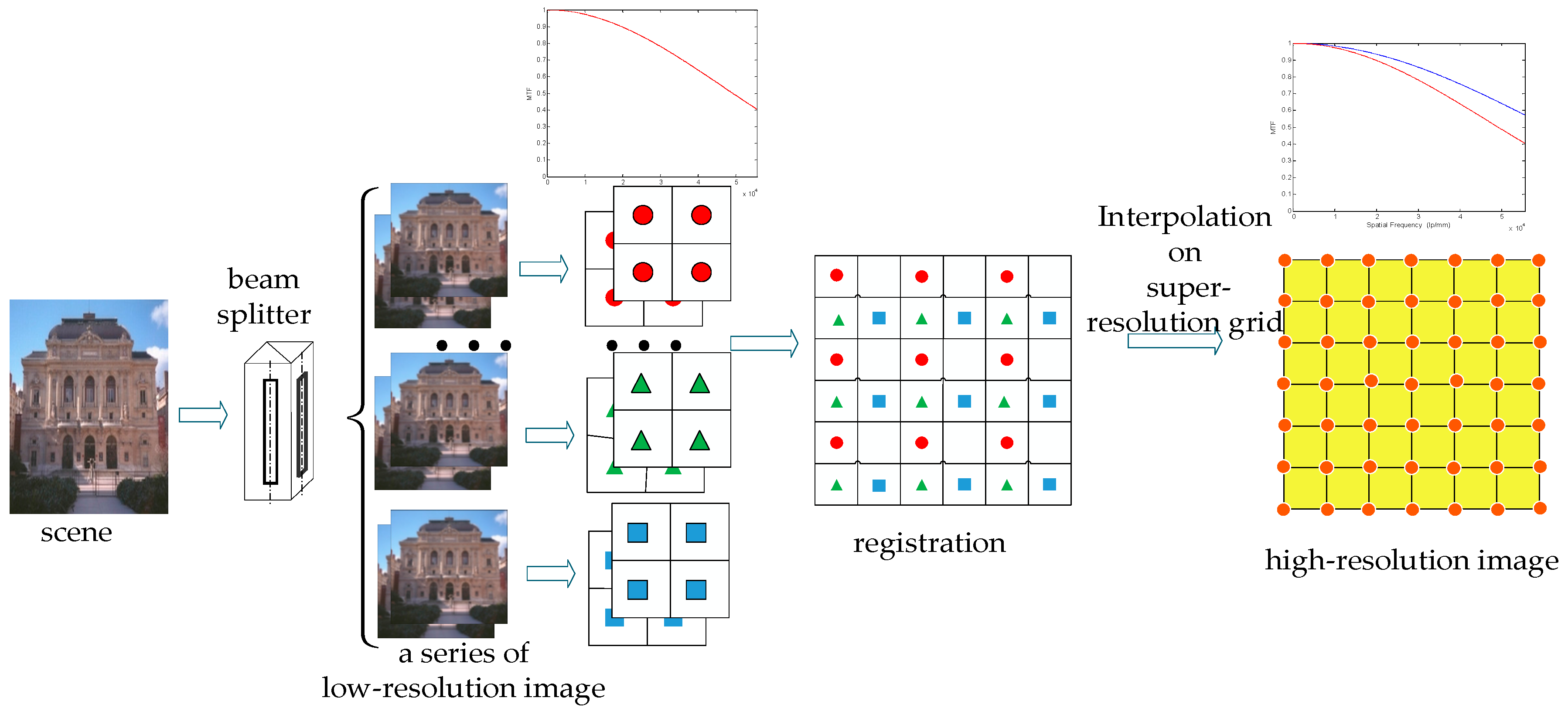
The technique of subpixel dynamic super-resolution imaging can overcome the under-sampling effect partially without changing new charge coupled device (CCDs) [4,5]. It use a set of undersampled (aliased) low-resolution (LR) images with subpixel shift to reconstruct a high-resolution (HR) image [6,7], namely oversampling operation (Figure 1). It aims to reconstruct the high-frequency contents which are commonly confused with the low-frequency contents in the LR images accessed by oversampling operation [8]. There have been proposed many subpixel imaging systems according to the oversampling operation formats. For example, the Canadian Defense Research Organization developed a high-performance micro-scanning imaging system for the application of infrared focal plane devices [9], which is a type of technique that doubles the resolution of the staring array imaging device. This technique can acquire multi-frame images of the same scene and detect the phase shift at each time. The French National Center for Space Research (CNES) applied the technique of subpixel imaging to Systeme Probatoire d’Observation dela Tarre 5 (SPOT5) satellites [10], which resulted in an increase in imaging resolution from 5 m to 3 m. The hot spot recognition system (HSRS) [11] sensor, which was developed by German Aerospace Center, and ADS40 [12] digital aerial remote-sensing camera, which was developed by the Lycra company, have adopted the similar technique of subpixel imaging. There are lots of analyses that come forth to evaluate the performance of such subpixel imaging methods. Wang discussed qualitatively the effect of micro-scanning modes on the quality of the image [13,14,15]. Zhang [16] introduced a super-resolution imaging system with oversampling technique. Hadar [17] analyzed the sampling performance of the CCD. However, this study did not mention the conditions under which the CCD reaches its sampling limit, and there was no analysis of the super-resolution reconstruction performance for multiple subpixel images.
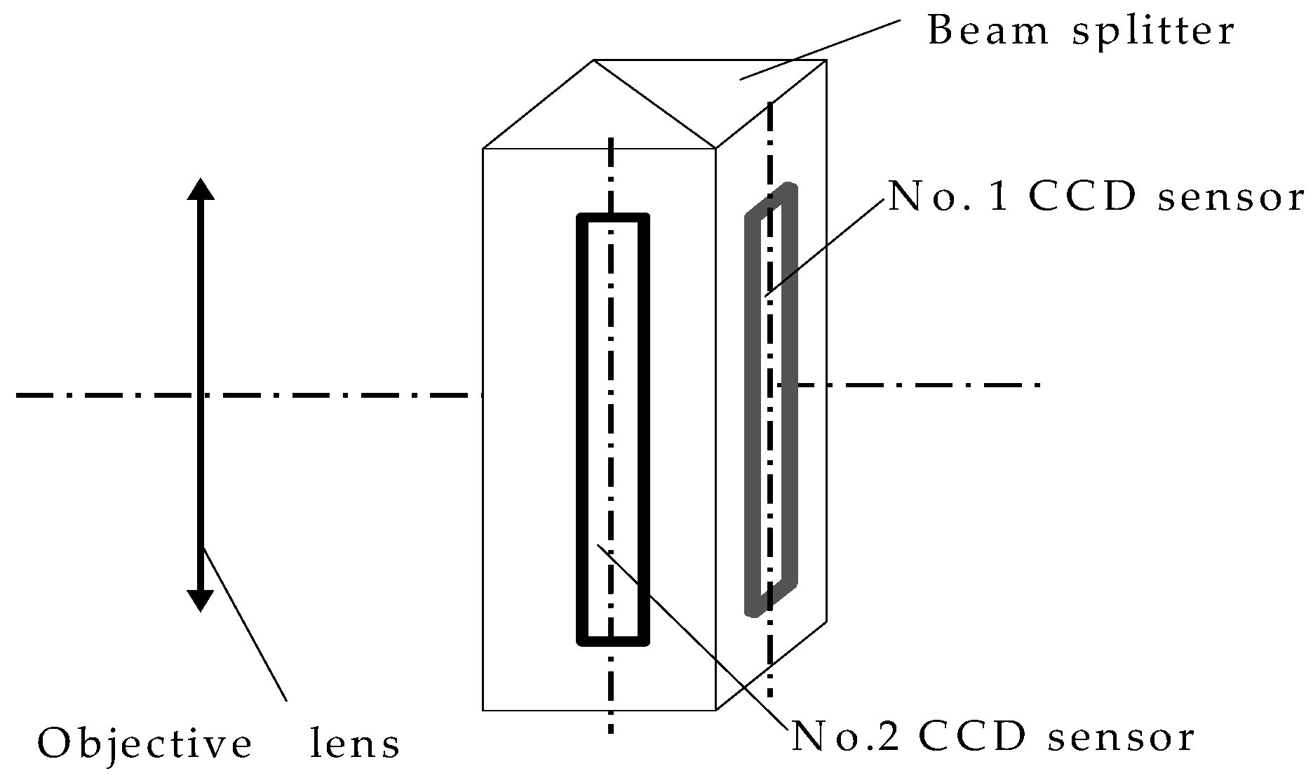
Liu [18] proposed another subpixel imaging technique (Figure 2) using a beam splitter to divide the light into two orthotropic beams. A pair of linear array CCD detectors are set up in the two imaging plane positions around the beam splitter with the staggered subpixel-level distance in the linear array direction. So a pair of conjugate images (called a subpixel image pair) would be simultaneously got by the CCD pair via this linear push-broom imaging system for the moving scenes. Through super-resolution processing, a new image with higher spatial resolution in the linear array direction would be constructed [19,20,21].
However, Liu’s work [18] only focused on the CCD sensors. Our subsequent research has updated the subpixel imaging system with TDI-CCDs. Considering MTF is the popular evaluating indicator for the imaging system, this paper proposes MTF analysis method based on discrete spatial oversampling for TDI–CCD subpixel imaging system. In Section 2, the improvement performance of MTF under the over-sampling conditions of subpixel dynamic super-resolution imaging is analyzed for CCD and TDI-CCD linear array in turn. In addition, the conditions of sampling in the limitations of the enhancement of MTF based on both linear CCD and TDI–CCD are given. These two cases are simulated and verified in Section 3. Finally, concluding remarks are presented in Section 4.
2. Sampling MTF of Subpixel Dynamic Super-Resolution Imaging
2.1. Partition Method of CCD
The most important common feature of the crystal’s inner structure is the periodicity of the molecules (atoms and ions) in the space [22]. The Wigner–Seitz cell is the smallest periodic unit of lattice, which is selected according to the following method: in the space lattice, take any node as the origin point; select all nodes near the origin point (if necessary, then consider the second nearest neighbor) and then draw the perpendicular bisectors of these lines [23] to form a rectangle spatial unit surrounded by these perpendicular bisectors (Figure 3) [24,25,26].
Considering the similarity characteristics between the inherent periodicity of CCD pixel spatial distribution and the Wigner–Seitz lattice (Figure 3), the lattice division theory can be used to describe the spatial sampling function of CCD with the traditional square shape (Figure 3a) or the other irregular shapes (Figure 3b). Solid line boxes are regarded as Wigner-Seitz lattice.
Setting the center distance of the pixel in every CCD as p, the pixel size is c, due to now most of the CCD duty cycles tend to 100% because of the use of microlens, c/p = 1. Therefore, we defined the Wigner–Seitz function , normalized with respect to the area of the Wigner–Seitz (WS) lattice as the following:
2.2. MTF of Over-Sampling with Linear CCDs
Assuming the linear CCD pixel size is p and its duty cycle is 100%, the over-sampling result of CCD pair in Figure 2 with the staggered offset a can be shown in Figure 4c.
We selected the center of each CCD pixel as the coordinate origin to establish a coordinate system. For the results from the new sampling, the Wigner–Seitz lattice is asymmetric. The intervals of Wigner–Seitz lattice are: .
The MTF of the sampling results is (The derivation details can be found in Appendix A):
For obtaining the condition of limitation, we set , the result is as below:
As Equation (3) can be applied to all types of , when and , may has the maximal value.
According to the above analysis, assuming that there are n pair of linear CCDs participated in the subpixel imaging with the staggered offset values of respectively, the over-sampling MTF can reach its maximal value when . (The detailed derivation is shown in Appendix A).
2.3. MTF of Over-Sampling with TDI–CCD
Comparing with CCD, the output signal of TDI-CCD pixel is the accumulation from multiple CCD linear arrays for the same scene during the scanning process to improve the response signal-noise rate (SNR) [27]. Actually, there often exists the drift angle caused by the influence of the space-borne camera. Let represent the moving speed of the target (or the push-broom canning direction of camera), the angle between and TDI integral direction is the drift angle :
where is the velocity component of in the direction of the CCD linear array; and is the velocity component of in the TDI integral direction (Figure 5b).
If the TDI–CCD line scanning speed and the target speed of motion is not synchronized, which may cause the image shift along the drift angle . Therefore, the output response of the pixel is:
where pixel’s center distance of the TDI–CCD is p (the length is same as the width); M is the TDI integral stages; is the synchronization accuracy; a is the difference between the image scanning speed and the TDI charge transfer rate.
The Fourier transform of is:
For oversampling in the imaging of TDI–CCD, the shifted distance is b in the vertical distance, assuming that the shifted distance is a in the horizontal direction (Figure 6).
A square and a triangle in Figure 6a are regarded as a basic unit, with the dashed box shown in the lower right corner. Using the division method of Wigner–Seitz cell interpolation, the regular square’s lattices are obtained and shown in Figure 6b.
The Wigner–Seitz function of TDI–CCD is equal to when and . In other cases, it is 0.
The modulation transfer function (MTF2) of the sampling results from two TDI-CCD is (The derivation details can be found in Appendix A):
For obtaining the condition of limitation, setting , we can obtain the following:
Then setting , thus we can obtain:
As Equations (8) and (9) are applicable to all of and , when and , the MTF2(a, b) has a maximum value when and .
Similar to analysis in Section 2.2, when there are n image pairs generated from TDI–CCD with shift distance and respectively. From the derivation process in Appendix A, when and , reach its maximum value.
3. Experiments
We have verified our analysis result above via mathematical simulation and subpixel image pairs from the real imaging system.
3.1. Simulation Analysis
3.1.1. Simulation of Subpixel Imaging with Linear CCD
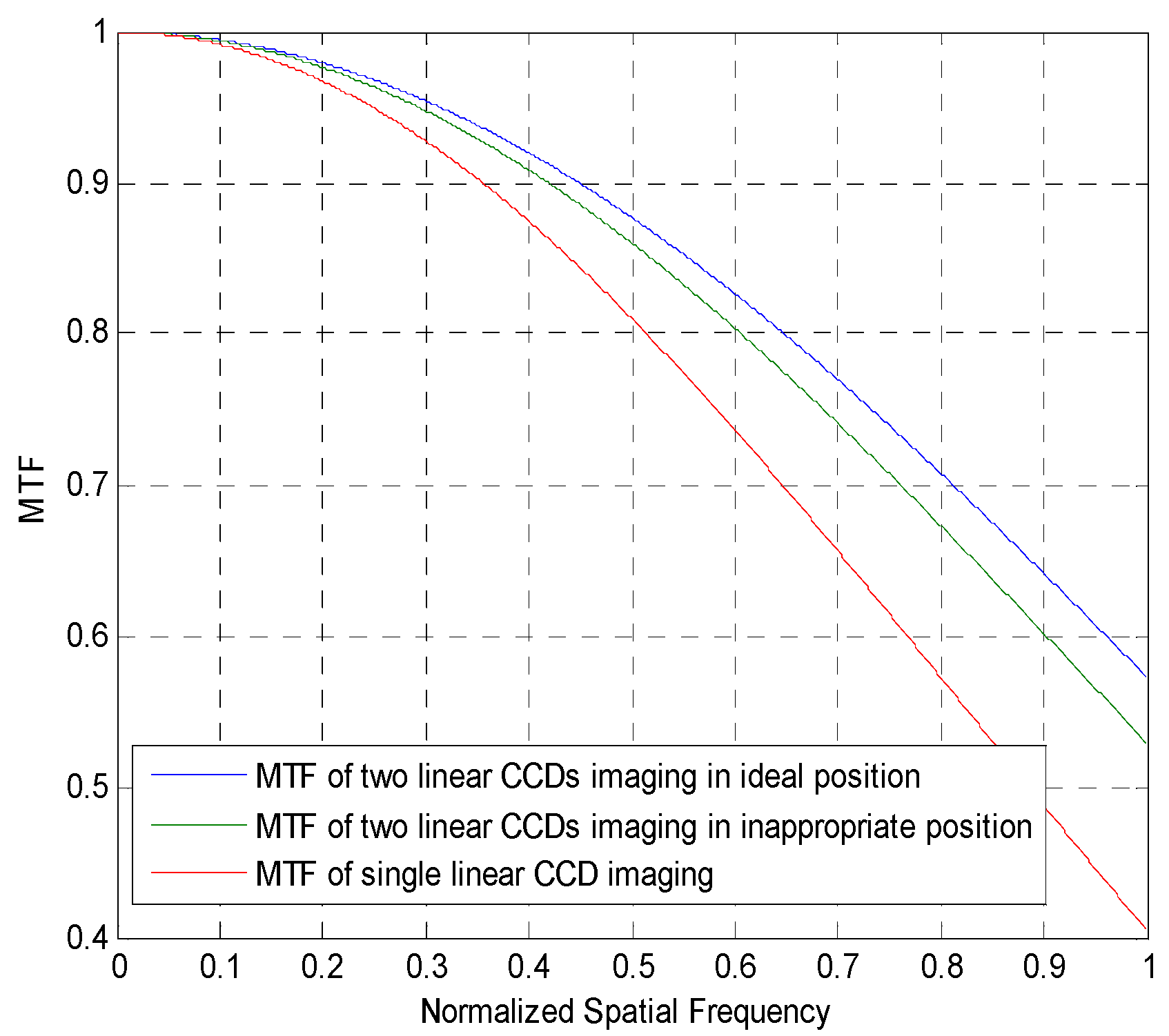
The MTF simulation results according to Section 2.2 with the normalized pixel size p are shown in Figure 7.
The blue curve represents the sampling MTF of the linear CCD pair with the ideal staggered distance . The green curve represents the sampling MTF with . The red curve is the sampling MTF from a single linear CCD.
From Figure 7, we can see the MTF value at Nyquist frequency are 0.5732, 0.5388 and 0.4053 respectively. So, subpixel imaging apparently does improve MTF when the linear CCD pair are staggerd with ideal distance of half a pixel size, which is consistent with theoretical result in Section 2.2.
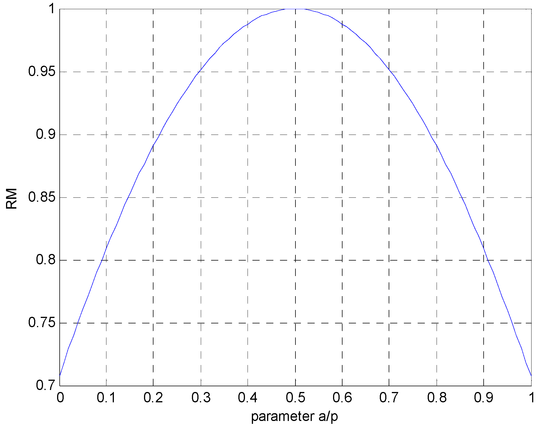
In order to quantitatively evaluate the influence due to the misaligned sampling points on the MTF in subpixel imaging, we will use the parameter RM which is the ratio of to under the Nyquist frequency as the basis for the evaluation,
where represents the MTF of the sampling point at any position a, which , represents the ideal MTF.
From Figure 8, we can see obviously that a = p/2 is the ideal position, where MTF has the maxim value and RM = 1. The more the distance of a deviates from the ideal location, the lower the RM value.
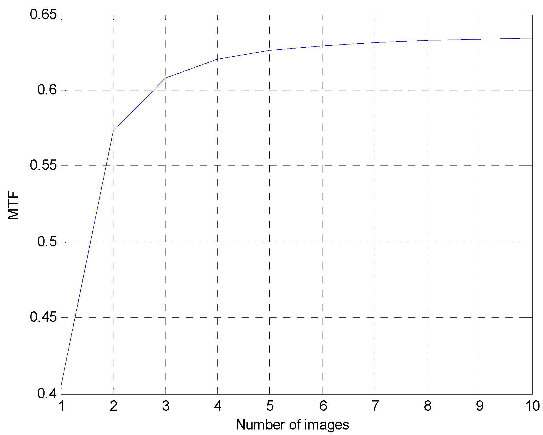
Figure 9 shows the value of MTF at the Nyquist frequency in the subpixel imaging system with multiple linear CCDs that satisfy the ideal sampling condition ai = p/2n according to result in Section 2.2. MTF appears an exponential growth trend with the imaging pairs number of linear CCDs. So, if we want to get a high resolution image through sub-pixel dynamic super-resolution imaging, 3 or 4 subpixel image pairs may be the most appropriate choice.
3.1.2. Simulation of Subpixel Imaging with Linear TDI–CCD
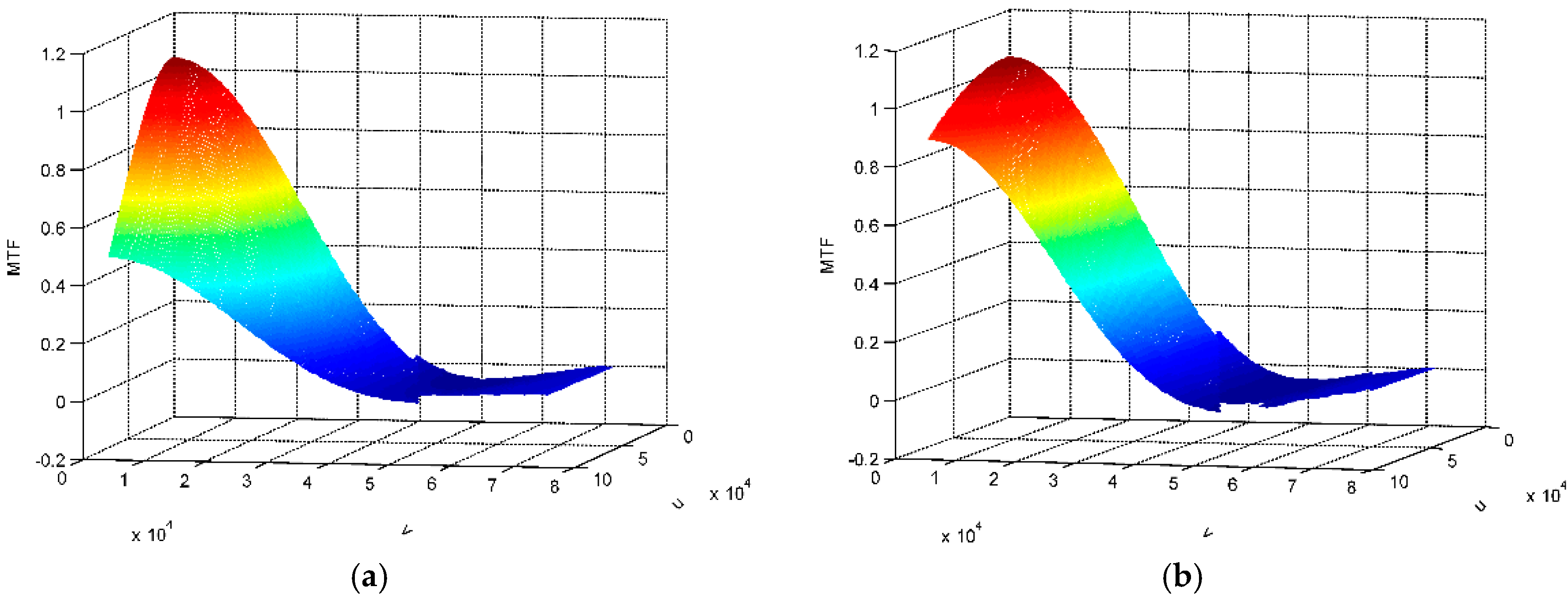
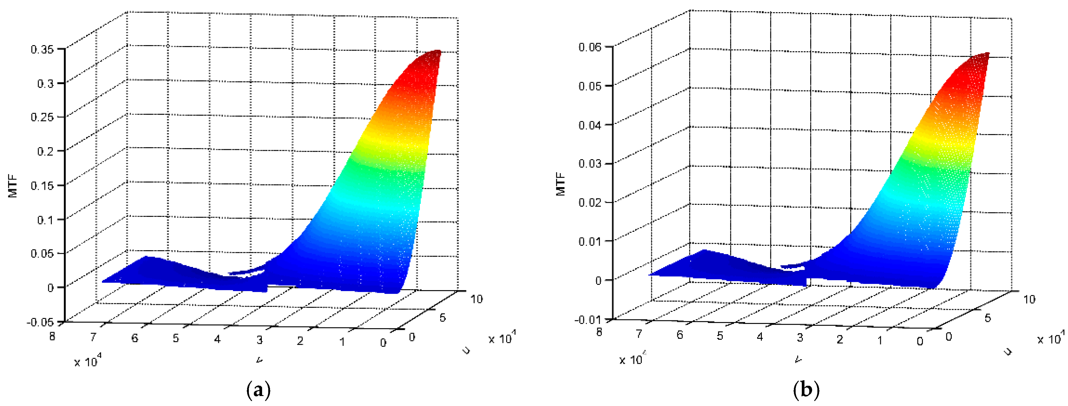
As using TDI will increase the effect of a mismatch in speed, the actual drift angle is very small (0–0.3°) when . In order to facilitate simulation, we set and θ = 0.15°. Some other parameters are set according to ZY-3 satellite nadir camera in Table 1. The MTF can draw the surface with changes in u and v according to results in Section 2.3, as shown in Figure 10.
Figure 10a shows the MTF of single TDI-CCD, Figure 10b shows the TDI-CCD sampling points in the best position when , Figure 10c shows the result with the serious offset of , Figure 10d shows the result with a minor offset of . It can be seen that the MTF at Nyquist frequency in the best position is significantly better than the other two graphs from these results. To highlight their differences, Figure 11a,b give the differences between MTF in Figure 10b,c, MTF in Figure 10b,d respectively. We can suppose that if subpixel imaging technology were applied in ZY-3, the resolution will be increased by almost 2 times at best under the condition of accurate imaging position. Although this is only a theoretical simulation, the resolution should also be clearly improved in the application of remote sensing cameras.
3.2. Verification of Real Subpixel Imaging System
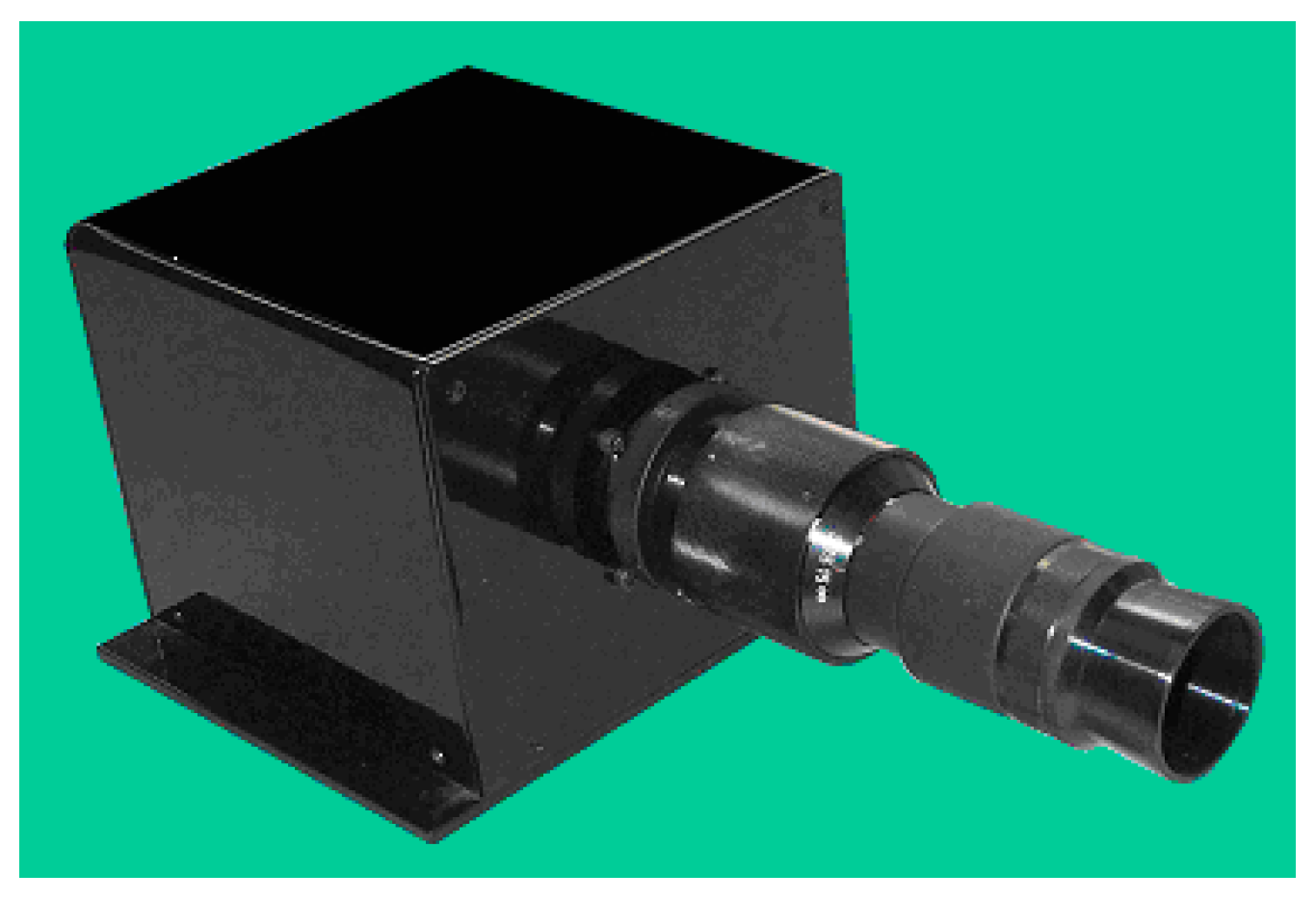
We have realized a subpixel camera according to Figure 2 using IL-E2 TDI-CCDs (Figure 12). The Table 2 gives the main indexes of camera and TDI-CCD. TDI–CCD line scanning speed and the target speed of motion is synchronized in this subpixel imaging.
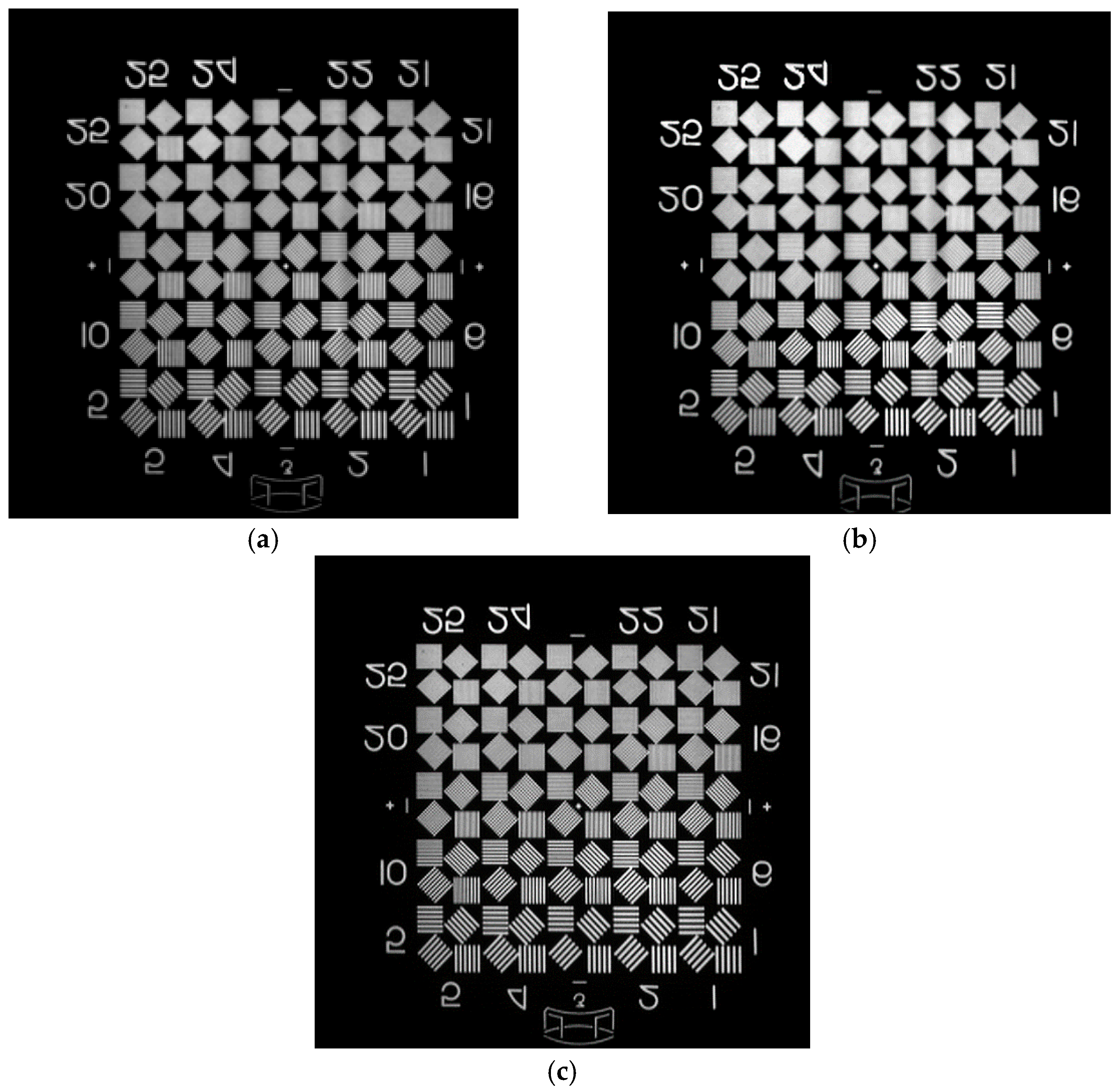
We used WT1005-62 transmitted resolution board to examine the MTF of this subpixel imaging system. Figure 13b reveals the reconstruction result of the image pair which has an inexact offset of half a pixel based on projections onto convex sets (POCS) algorithm. Figure 13c shows the same processing result of the image pair with the exact offset of half a pixel.
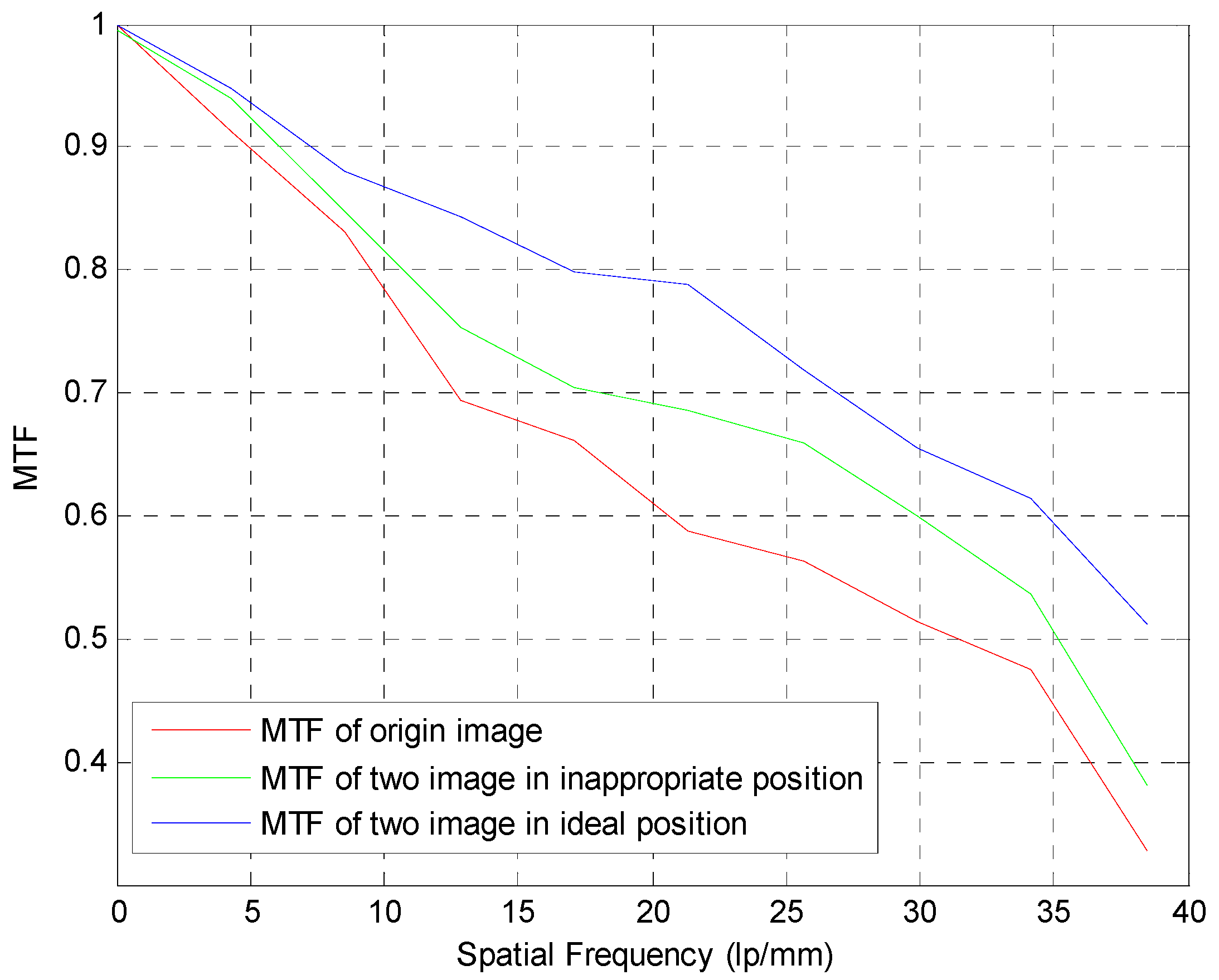
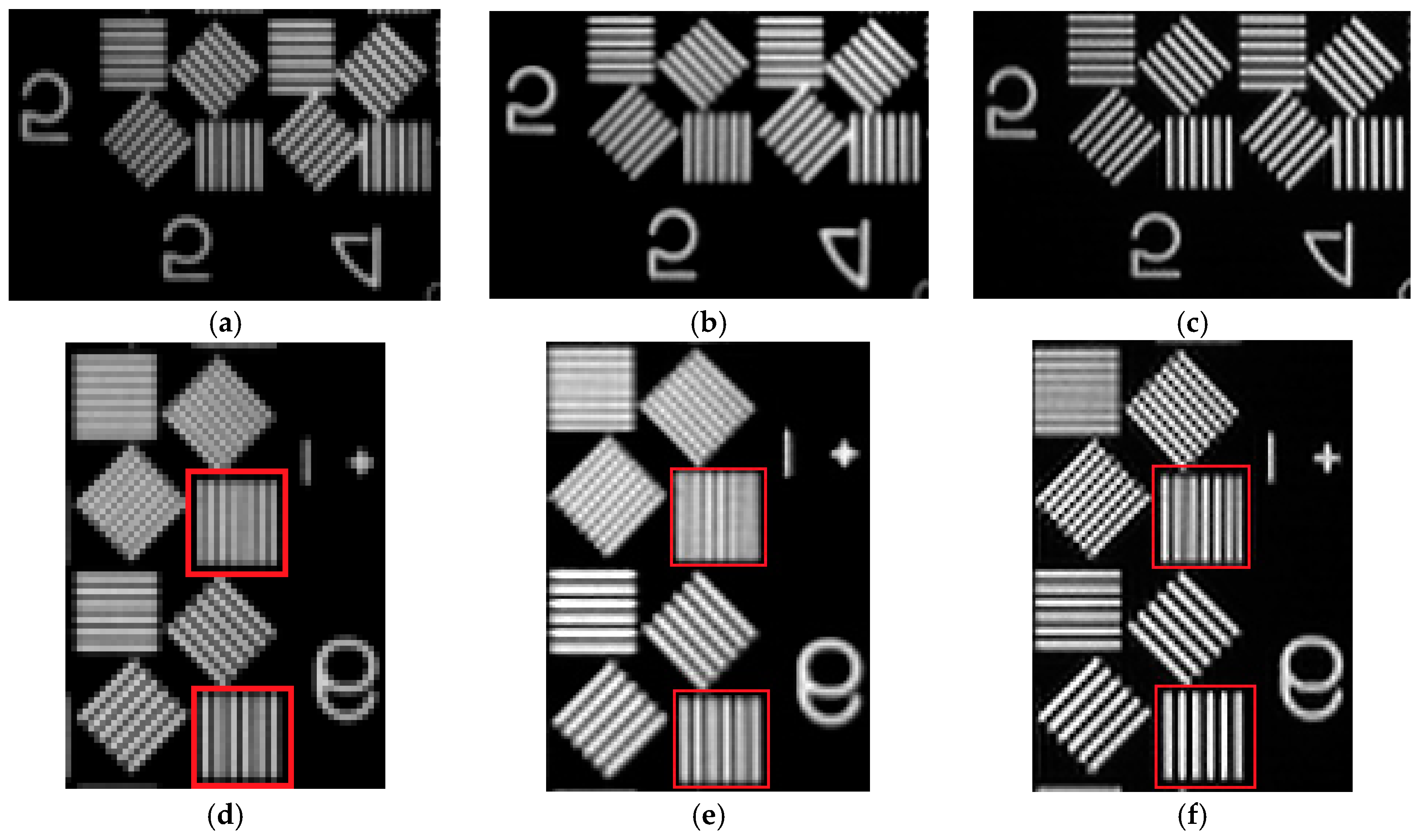
Figure 14 demonstrates more details with the 1:1 view. We found that the brightness contrast of Figure 14b is still better than Figure 14a, although the contour information is still indistinct. The resolution of Figure 14c is clearly improved, especially in the left second and fourth pairs of lines in the first row. There are many gray and indistinct regions in Figure 14d, with Figure 14e being clearer than the origin image despite the continuous presence of vague edges. In Figure 14f, each pair of lines can be clearly distinguished, especially those in the red box and in 45° direction. The experimental results show that the image quality of two images when taken in the ideal position is better than in the non-ideal position. A half pixel is the best imaging offset between two images. At the same time, this result is supported by the simulation results from the comparison of MTF (Figure 15).
4. Conclusions
In this paper, we analyzed the MTF in TDI–CCD subpixel dynamic super-resolution imaging using a beam splitter. Firstly, we established the oversampling MTF calculation model for the imaging system using linear CCD with the subpixel-level staggered distance in the CCD array direction. Following this, the oversampling MTF calculation model for the subpixel imaging system of TDI–CCD is deduced by adding the subpixel-level staggered distance in the push-broom scanning direction. Furthermore, constraints due to the CCD sampling limit in the MTF enhancement were given. In fact, the MTF calculation model proposed in this paper can be applied to other sub-pixel imaging systems. Finally, the experimental results were relatively consistent with the theory, which proves that this theory can provide a mathematical basis for the super-resolution reconstruction process. It points to future directions for the design standards of high resolution remote sensing cameras.
Acknowledgments
The authors would like to thank the reviewers of this manuscript for their helpful comments and suggestions. This work was supported by the National High Technology Research and Development Program of China (863 Program, grant No. 2014AA7026082), the Natural Science Foundation of Beijing, China (grant No. 4152045), the National Natural Science Foundation of China (grant No. 61071148) and the Science Research Project of CUC (grant No. 3132014XNG1417, 3132016XNG1612).
Author Contributions
Kun Gao and Lu Han proposed the model; Hongmiao Liu and Zeyang Dou derived some formulas of the model; Guoqiang Ni and Yingjie Zhou completed some figures using a program.
Conflicts of Interest
The authors declare no conflicts of interest.
Appendix A
Appendix A.1. Derivation Details of Function (2)
Wigner-Seitz (WS) cell as the following:
According to Equation (A1), the Fourier transformation of is:
The real part of is:
In order to preserve the convenience of the transfer function analysis method, Park [28] and Hadar [29] deduced the pixel function independently. This is determined by the process of discrete sampling in the CCD array through different methods, with the resultant pixel function being:
The Fourier transform of s(x) is:
From Equations (A3) and (A5), the average modulation transfer function (MTF) of the sampling results from two linear CCD is:
In Equation (A6), represents the revolution; represents the product; represents the Fourier transformation and .
Appendix A.2. Derivation Details of
Firstly, the intervals of Wigner–Seitz lattice are as follows:
The Fourier transformation of is:
The real part of W(f) is:
From Equations (A5) and (A8), the average MTF of the sampling results of n pairs of the images from linear CCD is:
Appendix A.3. Derivation Details of Function (7)
The Wigner–Seitz function of TDI–CCD is equal to when and . In other cases, it is 0. Therefore, its Fourier transformation is:
The real part of is:
Therefore:
Appendix A.4. Derivation Details of
Wigner–Seitz function of TDI–CCD is equal to when intervals of x direction are:
The intervals of y direction are:
In other cases, it is 0. Therefore, its Fourier transformation is:
The real part of is:
Therefore:
References
- Jerri, A.J. The Shannon sampling theorem—Its various extensions and applications: A tutorial review. Proc. IEEE 1977, 65, 1565–1596. [Google Scholar] [CrossRef]
- Jun, Z.; Wei, H.; Xiaodong, Z.; Guofan, J. Design of a low F-number freeform off-axis three-mirror system with rectangular field-of-view. J. Opt. 2015, 17, 015605. [Google Scholar]
- Wei, H.; Jun, Z.; Tong, Y.; Guofan, J. Construction method through forward and reverse ray tracing for a design of ultra-wide linear field-of-view off-axis freeform imaging systems. J. Opt. 2015, 17, 055603. [Google Scholar]
- He, L.Y.; Liu, J.H.; Li, G. Super resolution of aerial image by means of polyphase components reconstruction. Acta Phys. Sin. 2015, 64. [Google Scholar]
- Hu, S.; Zhang, S.; Zhang, A. Hyperspectral Imagery Super-Resolution by Adaptive POCS and Blur Metric. Sensors 2017, 17, 82. [Google Scholar] [CrossRef] [PubMed]
- Rajan, D.; Chaudhuri, S. Generalized interpolation and its applications in super-resolution imaging. Image Vis. Comput. 2001, 19, 957–969. [Google Scholar] [CrossRef]
- Tom, B.C.; Katsaggelos, A.K. Resolution enhancement of monochrome and color video using motion compensation. IEEE Trans. Image Process. 2001, 10, 278–287. [Google Scholar] [CrossRef] [PubMed]
- Borman, S.; Stevenson, R.L. Spatial Resolution Enhancement of Low-Resolution Image Sequences—A Comprehensive Review with Directions for Future Research. 1998. Available on line: https://www.researchgate.net/profile/Robert_Stevenson3/publication/2461146_Spatial_Resolution_Enhancement_of_Low-Resolution_Image_Sequences_-_A_Comprehensive_Review_with_Directions_for_Future_Research/links/5564757708ae9963a120209a/Spatial-Resolution-Enhancement-of-Low-Resolution-Image-Sequences-A-Comprehensive-Review-with-Directions-for-Future-Research.pdf (accessed on 30 August 2017).
- Jean, F.; Paul, C. Realization of a fast microscanning device for infrared focal plane arrays. In Proceedings of the SPIE Infrared Imaging Systems: Design, Analysis, Modeling, and Testing, Orlando, FL, USA, 8–14 April 1996; Volume 2743, pp. 185–196. [Google Scholar]
- Latry, C.; Rouge, B. SPOT5 thr mode. In Proceedings of the SPIE on Earth Observinci System, San Diego, CA, USA, 19–24 July 1998; Volume 3439, pp. 480–491. [Google Scholar]
- Skrbek, W.; Lorenz, E. HSRS: An infrared sensor for hot spot detection. In Proceedings of the SPIE Infrared Soaceborne Remote Sensing, San Diego, CA, USA, 18 November 1998; pp. 167–175. [Google Scholar]
- Sandau, R.; Braunecker, B.; Driescher, H. Design principles of the LH Systems ADS40 airborne digital sensor. In Proceedings of the International Archives of Photogrammetry and Remote Sensing, Amsterdam, The Netherlands, January 2000; Volume 33, pp. 258–265. [Google Scholar]
- Wang, X.; Zhang, J.; Feng, Z. Analysis of improvement amount of typical microscanning modes to IR imagery quality. Infrared Phys. Technol. 2005, 46, 412–417. [Google Scholar] [CrossRef]
- Wang, X.; Hua, H. Theoretical analysis for integral imaging performance based on microscanning of a microlens array. Opt. Lett. 2008, 33, 449–451. [Google Scholar] [CrossRef] [PubMed]
- Wang, X.; Zhang, J.; Chang, H. Assessment of the Performance of Staring Infrared Imaging Array Based on Microscanning Modes. Int. J. Infrared Millim. Wave 2004, 25, 905–916. [Google Scholar] [CrossRef]
- Zhang, X.; Liu, Y.; Zhang, J. Super-resolved imaging system with oversampling technology. In Proceedings of the 3rd International Symposium on Advanced Optical Manufacturing and Testing Technologies, Chengdu, China, 8–12 July 2007; International Society for Optics and Photonics: Bellingham, WA, USA, 2007. [Google Scholar] [CrossRef]
- Hadar, O.; Boreman, G.D. Oversampling requirements for pixelated-imager systems. Opt. Eng. 1999, 38, 782–785. [Google Scholar]
- Liu, X.; Wen, D.; Qiao, W. Subpixel imaging technique. In Proceedings of the SPIE on Sensors and Controls for Intelligent Machining, Boston, MA, USA, 19–22 September 1999; Volume 3832, pp. 158–162. [Google Scholar]
- Alam, M.S.; Bognar, J.G.; Hardie, R.C.; Yasuda, B.J. Infrared image registration and high-resolution reconstruction using multiple translationally shifted aliased video frames. IEEE Trans. Instrum. Meas. 2000, 49, 915–923. [Google Scholar] [CrossRef]
- Lim, W.; Park, M.; Kang, M.G. Spatially adaptive regularized iterative high resolution image reconstruction algorithm. In Proceedings of the VCIP2001, Photonics West, San Jose, CA, USA, 20 January 2001; pp. 20–26. [Google Scholar]
- Hardie, R.C.; Barnard, K.J.; Bognar, J.G.; Armstrong, E.E.; Watson, E.A. High-resolution image reconstruction from a sequence of rotated and translated frames and its application to an infrared imaging system. Opt. Eng. 1998, 37, 247–260. [Google Scholar]
- Vainshtein, B.K. Modern Crystallography: Fundamentals of Crystals, Symmetry and Methods of Structural Crystallography. Acta Crysrallogr. 1995, 51, 234–235. [Google Scholar] [CrossRef]
- Olivas, A.; Antúnez-García, J.; Fuentes, S. Electronic properties of unsupported trimetallic catalysts. Catal. Today 2014, 220, 106–112. [Google Scholar] [CrossRef]
- Song, H.F.; Liu, H.F. Modified mean-field potential approach to thermodynamic properties of a low-symmetry crystal: Beryllium as a prototype. Phys. Rev. B 2007, 75, 245126. [Google Scholar] [CrossRef]
- Wasserman, E.; Stixrude, L.; Cohen, R.E. Thermal properties of iron at high pressures and temperatures. Phys. Rev. B 1996, 53, 8296. [Google Scholar] [CrossRef]
- Jiuxun, S.; Lingcang, C.; Qiang, W. Equivalence of the analytic mean-field potential approach with free-volume theory and verification of its applicability based on the Vinet equation of state. Phys. Rev. B 2005, 71, 024107. [Google Scholar] [CrossRef]
- Qiaolin, H.; Xiangmin, L. Application of TDICCD on real-time earth reconnaissance satellite. In Proceedings of the International Society for Optics and Photonics, Beijing, China, 16–19 September 1998; pp. 93–104. [Google Scholar]
- Park, S.K.; Schowengerdt, R.; Kaczynski, M.A. Modulation-transfer-function analysis for sampled image systems. Appl. Opt. 1984, 23, 2572–2582. [Google Scholar] [CrossRef] [PubMed]
- Hadar, O.; Dogariu, A.C.; Boreman, G.D. Angular dependence of sampling MTF. In Proceedings of the 10th Meeting on Optical Engineering in Israel, Jerusalem, Israel, 2–6 March 1997; pp. 536–547. [Google Scholar]
Figure 1.
Schematic of super-resolution technique.

Figure 2.
Schematic of sub-pixel imaging using beam splitter.

Figure 3.
Partition results of the charge coupled device (CCD) sampling interval. (a) Partition result of traditional CCD; (b) Partition result of irregular CCD.
Figure 3.
Partition results of the charge coupled device (CCD) sampling interval. (a) Partition result of traditional CCD; (b) Partition result of irregular CCD.
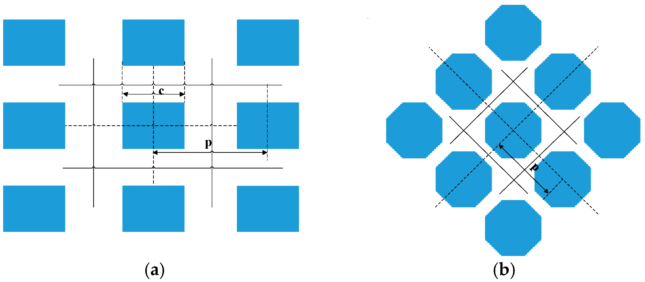
Figure 4.
Sampling results of linear CCD pair. (a) Sampling of the first linear CCD; (b) Sampling of the second linear CCD; (c) Sampling results of the first linear CCD and the second linear CCD.
Figure 4.
Sampling results of linear CCD pair. (a) Sampling of the first linear CCD; (b) Sampling of the second linear CCD; (c) Sampling results of the first linear CCD and the second linear CCD.
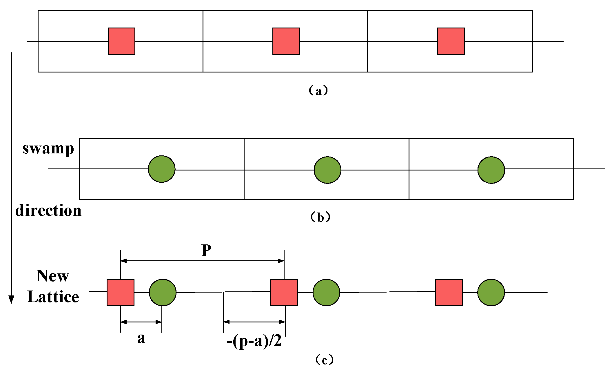
Figure 5.
Schematic of time delay integration (TDI)–CCD. (a) Operation mode of TDI-CCD; (b) The relationship between each velocity.
Figure 5.
Schematic of time delay integration (TDI)–CCD. (a) Operation mode of TDI-CCD; (b) The relationship between each velocity.
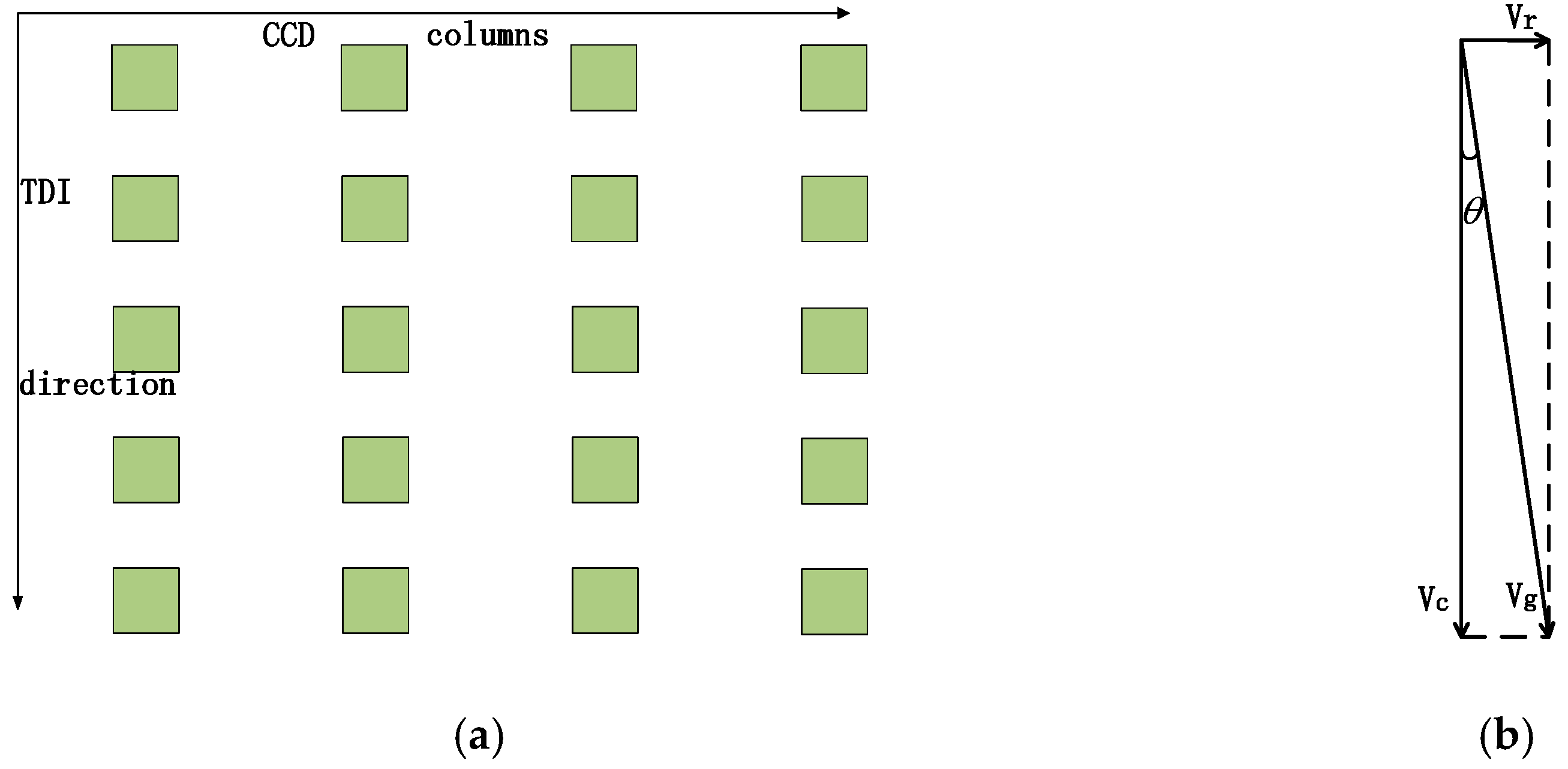
Figure 6.
Sampling results of TDI–CCD. (a) Sampling results of TDI-CCD pairs; (b) Sampling results of TDI-CCD pairs after partition.
Figure 6.
Sampling results of TDI–CCD. (a) Sampling results of TDI-CCD pairs; (b) Sampling results of TDI-CCD pairs after partition.
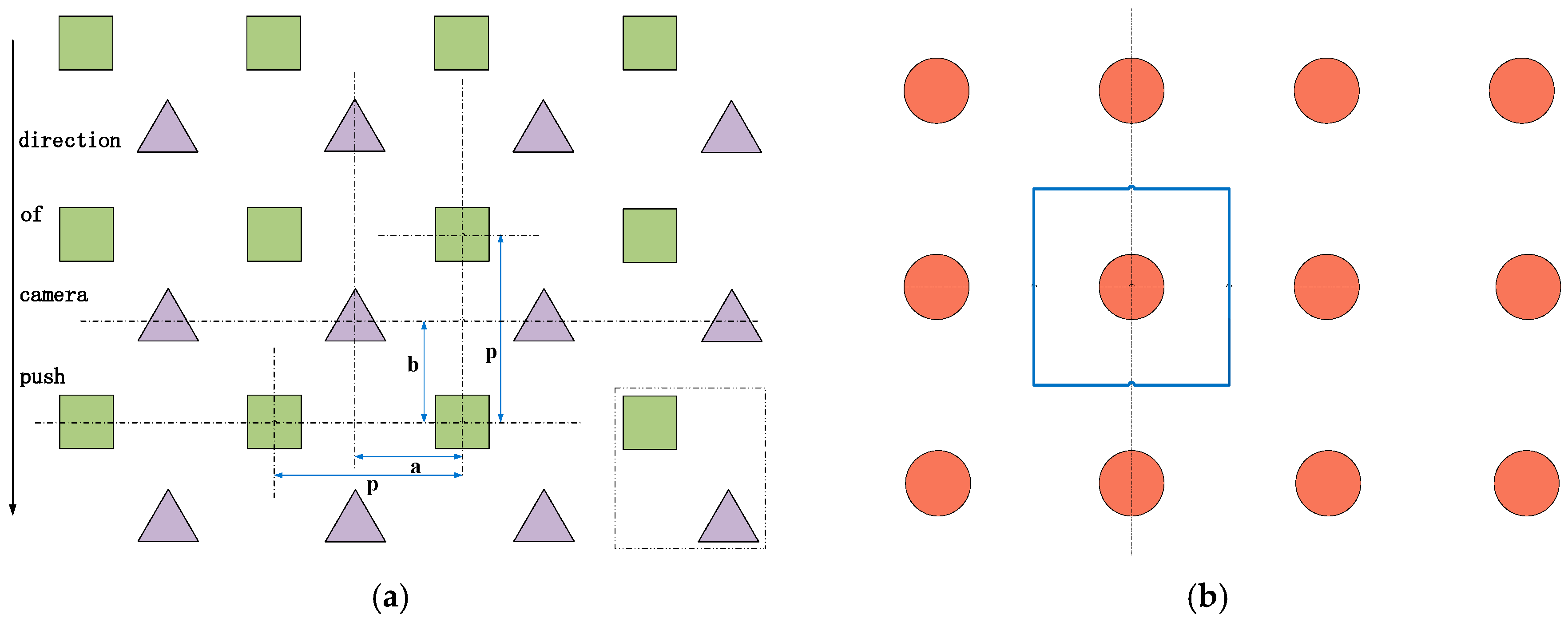
Figure 7.
MTF comparison of single linear CCD and subpixel linear CCD pair.

Figure 8.
Relation diagram between RM and sampling point location.

Figure 9.
MTF simulation result of the subpixel imaging system with multiple images.

Figure 10.
Modulation transfer function (MTF) of different sampling positions in TDI–CCD. (a) MTF of single TDI-CCD; (b) MTF of sampling points in the best position; (c) MTF of sampling points with the serious offset; (d) MTF of sampling points with the minor offset.
Figure 10.
Modulation transfer function (MTF) of different sampling positions in TDI–CCD. (a) MTF of single TDI-CCD; (b) MTF of sampling points in the best position; (c) MTF of sampling points with the serious offset; (d) MTF of sampling points with the minor offset.

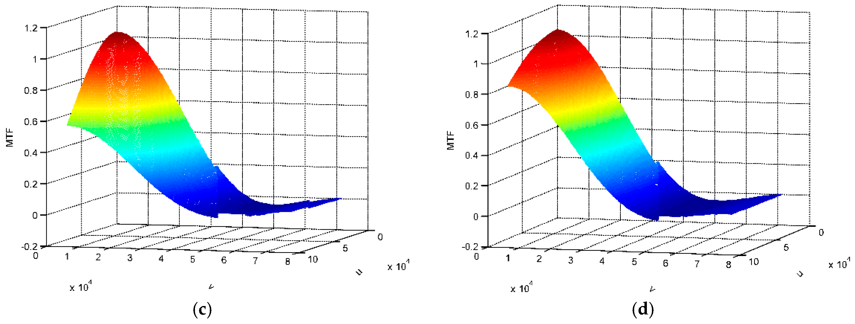
Figure 11.
MTF differences with different sampling positions. (a) MTF difference between Figure 10b,c; (b) MTF difference between Figure 10b,d.

Figure 12.
The contour of camera.

Figure 13.
Experimental results from subpixel imaging. (a) Origin image; (b) Results from super-resolution in the non-ideal position; (c) Results from the super-resolution in the ideal position.
Figure 13.
Experimental results from subpixel imaging. (a) Origin image; (b) Results from super-resolution in the non-ideal position; (c) Results from the super-resolution in the ideal position.

Figure 14.
Details of the experiment. (a) Part 1 of origin image; (b) Part 1 of Figure 14b; (c) Part 1 of Figure 14c; (d) Part 2 of origin image; (e) Part 2 of Figure 14b; (f) Part 2 of Figure 14c.

Figure 15.
MTF comparison of the experimental results.

Table 1.
Key technical parameters of the ZY-3 satellite nadir camera.
| Parameter | Index |
|---|---|
| Ground resolution | 2.1 m |
| Width | 51 km |
| MTF of Lab | 0.23 (71.5 lp/mm) |
| SNR | |
| Pixel size | 7 μm |
| TDI stages | 24 |
| CCD duty cyle | 100% |
Table 2.
Main indexes of camera and TDI-CCD.
| Parameter | Index |
|---|---|
| CCD type | IL-E2 TDI-CCD |
| Number of pixels | 2048 |
| Dynamic range | 1600:1 |
| Pixel size | 13 μm |
| TDI stages | 24 |
| Speed of valid data | 30 MHz |
© 2017 by the authors. Licensee MDPI, Basel, Switzerland. This article is an open access article distributed under the terms and conditions of the Creative Commons Attribution (CC BY) license (http://creativecommons.org/licenses/by/4.0/).
Share and Cite
MDPI and ACS Style
Gao, K.; Han, L.; Liu, H.; Dou, Z.; Ni, G.; Zhou, Y. Analysis of MTF in TDI-CCD Subpixel Dynamic Super-Resolution Imaging by Beam Splitter. Appl. Sci. 2017, 7, 905. https://doi.org/10.3390/app7090905
AMA Style
Gao K, Han L, Liu H, Dou Z, Ni G, Zhou Y. Analysis of MTF in TDI-CCD Subpixel Dynamic Super-Resolution Imaging by Beam Splitter. Applied Sciences. 2017; 7(9):905. https://doi.org/10.3390/app7090905
Chicago/Turabian StyleGao, Kun, Lu Han, Hongmiao Liu, Zeyang Dou, Guoqiang Ni, and Yingjie Zhou. 2017. "Analysis of MTF in TDI-CCD Subpixel Dynamic Super-Resolution Imaging by Beam Splitter" Applied Sciences 7, no. 9: 905. https://doi.org/10.3390/app7090905
Note that from the first issue of 2016, this journal uses article numbers instead of page numbers. See further details here.