LiDARgrammetry: A New Method for Generating Synthetic Stereoscopic Products from Digital Elevation Models

Abstract

There are currently several new technologies being used to generate digital elevation models that do not use photogrammetric techniques. For example, LiDAR (Laser Imaging Detection and Ranging) and RADAR (RAdio Detection And Ranging) can generate 3D points and reflectivity information of the surface without using a photogrammetric approach. In the case of LiDAR, the intensity level indicates the amount of energy that the object reflects after a laser pulse is transmitted. This energy mainly depends on the material and the wavelength used by LiDAR. This intensity level can be used to generate a synthetic image colored by this attribute (intensity level), which can be viewed as a RGB (red, green and blue) picture. This work presents the outline of an innovative method, designed by the authors, to generate synthetic pictures from point clouds to use in classical photogrammetric software (digital restitution or stereoscopic vision). This is conducted using available additional information (for example, the intensity level of LiDAR). This allows mapping operators to view the LiDAR as if it were stereo-imagery, so they can manually digitize points, 3D lines, break lines, polygons and so on.

1. Introduction

At present, there are a number of diverse techniques for generating digital elevation models (such as terrain or surface models) that do not require images to be directly captured. Some of these technologies that are widely used include LiDAR, echo sounder and laser scanner [1].

All these techniques can generate dense point clouds with defined spatial attributes. However, these point clouds cannot be displayed by classical methods of stereoscopic vision and, thus, they are incompatible with the software used in classic photogrammetric stations. This software usually allows us to visualize images with stereoscopic vision (using 3D glasses) to digitalize elements, such as points, lines or polygons. These tools are necessary for the process of cartographic production and they are not available in software for computing point clouds (with no 3D vision available). Therefore, when the images are not available, we cannot use photogrammetric software to conduct this process and a synthetic stereoscopic pair (photogrammetric model) must be generated from the available point cloud.

The adjective ‘synthetic’ is used to describe this stereoscopic pair for the following reason. As no radiometric information is available in the visible range, the generated image will have a specific characteristic provided by the sensor used (LiDAR intensity level, terrain reflectivity, etc.). This is achieved assigning a “false color” to the images obtained in the process in order to ensure correct 3D visualization [2].

LiDARgrammetry is a term coined by GeoCue for using the intensity information as the source data for generating stereo-models of the project area directly from the LiDAR data itself rather than from ancillary imagery. By creating appropriate stereo-pairs from the LiDAR intensity images, it is possible to generate stereo-models that can be directly exploited using existing photogrammetric workstations and the traditional photogrammetric workflow in areas, such as feature extraction or break line compilation [3].

LiDARgrammetry concerns the production of inferred stereo-pairs from LiDAR intensity images, which aims to stereo-digitize the spatial data in digital photogrammetric stations. The production of inferred stereo-pairs is based on the principle of stereo ortho-mates and the extraction of a derivative intensity image, in which an artificial x-parallax is introduced. Furthermore, other techniques have also developed in order to fully utilize the 3D nature of LiDAR data. LiDARgrammetry aims to quantify the derivative spatial data quality and the impact of the reduced photo-interpretative ability of LiDAR data with comparisons to typical photogrammetric stereo-models [4]. However, this relatively new approach has not been yet assessed properly.

The LiDARgrammetry technique is based on the inverse algorithm of the photogrammetric technique, which is namely the 3D dataset (point cloud) that is used to generate 2D information (synthetic images). Therefore, the resolution and definition of the images depend on the density (points per square meters) and radiometric characteristics (intensity level) of the LiDAR dataset as well as the resampling algorithm used. The images are generated as if they had been registered at a given position using the “base–height” ratio related to the dataset’s parameters, which are used as a base reference.

The objective of the work presented here is to design and develop a suitable methodology for generating and visualizing 3D images from point clouds. Within this context, the “radargrammetry” technique [5] can be considered, which is similar to the photogrammetric one as it allows us to display point clouds using photogrammetric stations via the generation of synthetic images.

The purpose of this methodology is to create an alternative (cheap and easy) method for photogrammetry in cases where it is not possible to use photogrammetry (for example, in adverse weather conditions).

Restitution is often applied in a considerable number of work environments, including engineering, architecture, archaeology and cartography. The different types of software for restitution allow the operator to identify some points, lines and polygons to create vector layers using 3D glasses. In general, the software used for processing point clouds does not allow this functionality. Thus, it is very useful to obtain a pair of synthetic pictures using the methodology that we propose in this article as these can be used to create these new layers. Digital restitution provides shapes and sizes for engineering and architecture as well as different-scaled maps of cities, continents or celestial objects. The present study used these techniques to develop a specific software, in order to generate synthetic images and obtain some break lines of interest, using digital restitution DIGI 3D software from a LiDAR flight (SHAKE, I+D project financed in public announcements) [6].

2. Methodology to Generate a Synthetic Image

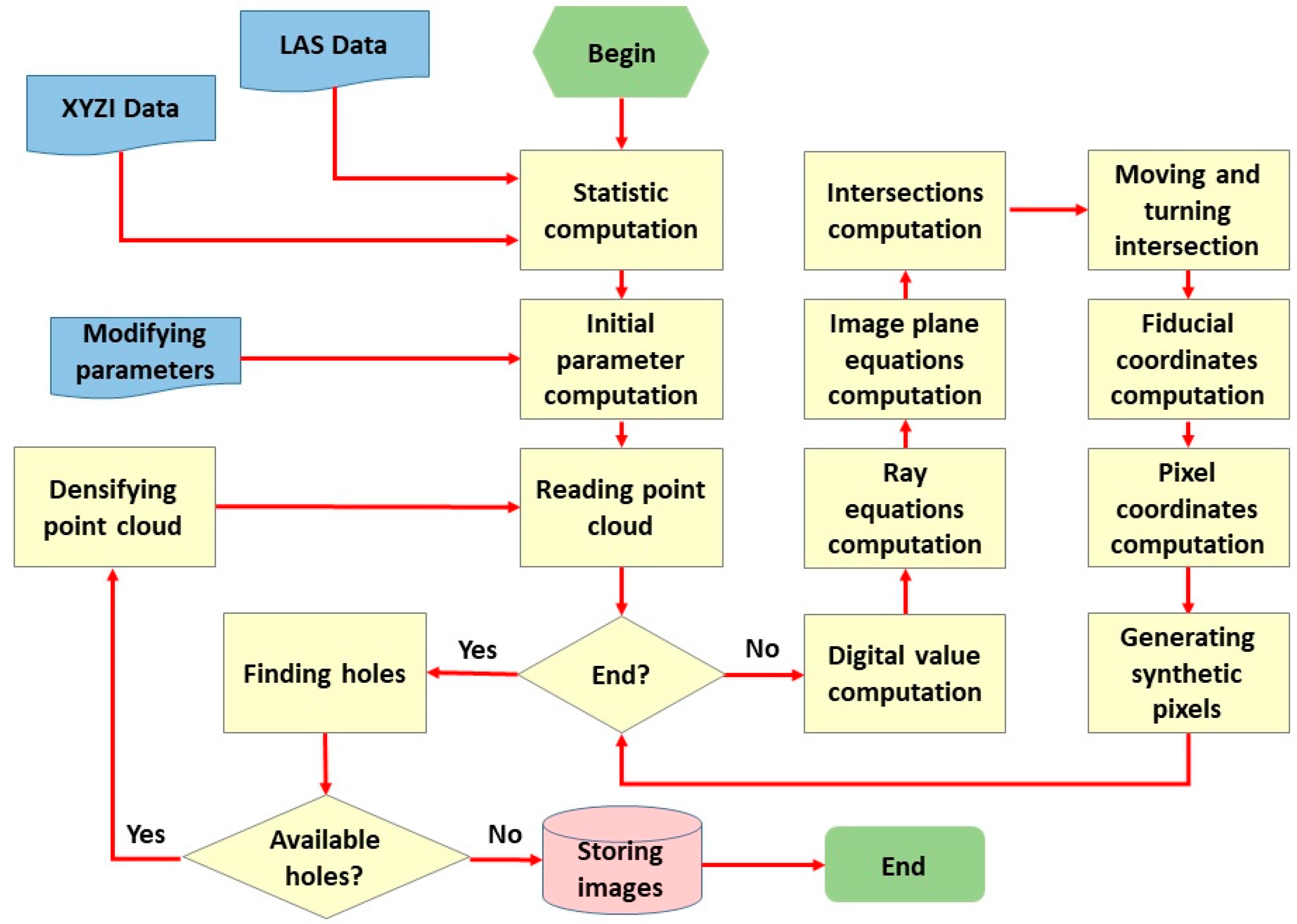
This paper describes a methodology that will allow us to extract photogrammetric images from any point cloud, which can then be used as input information. Figure 1 shows a block diagram of the methodology designed by the authors for generating synthetic images.

This methodology must be carried out in a series of phases.

2.1. Treatment of Initial Data

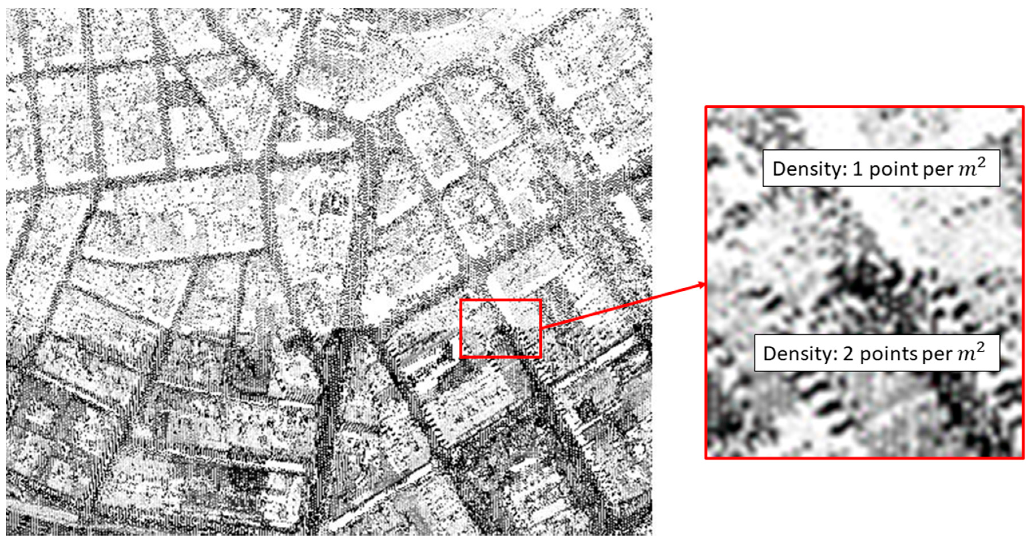
Initially, the starting data is a cloud of LiDAR points. The aspect of the point cloud can be seen in Figure 2, which is shown as the areas with a greater density of points (dark zones) when compared to other areas where there is a smaller density of points. The bottom part of Figure 2 shows a dark zone with a double density of points, which corresponds with the overlap zone for LiDAR flight (right zoom of Figure 2).

Usually, in this type of point cloud, the density is calculated in points per square meter, which is an average density for the whole cloud in practice.

The attributes that define a LiDAR point cloud are described below (this development is similar for any other type of point cloud):

• Planimetric coordinates $\left(X,Y\right)$ in a given reference system;
• Height ($Z$) in a given reference system;
• Intensity level or another attribute as reflectivity.

The point cloud could be irregular and, from it, two digital elevation models can be extracted:

∘

A digital surface model (or ground, if this is the case) using the planimetric coordinates $\left(X, Y\right)$ and the height $\left(Z\right)$. The mathematical expression is:

$$N_Z=\left\{\left(X_1,Y_1,Z_1\right),\left(X_2,Y_2,Z_2\right),\dots ,\left(X_n,Y_n,Z_n\right)\right\}.$$

(1)

∘

A digital elevation model, using the planimetric coordinates $\left(X, Y\right)$ and the intensity level $\left(I\right)$. The mathematical expression is:

$$N_I=\left\{\left(X_1,Y_1,I_1\right),\left(X_2,Y_2,I_2\right),\dots ,\left(X_n,Y_n,I_n\right)\right\}.$$

(2)

In both expressions, $n$ is the number of elements in a point cloud.

The main target of this procedural step is to obtain a good density and a well-distributed point cloud in order to be similar to a photogram where all pixels have a regular distribution and the distance between two contiguous pixels is always the same. Therefore, all white spaces are filled with new points that have an intensity level similar to their neighbors.

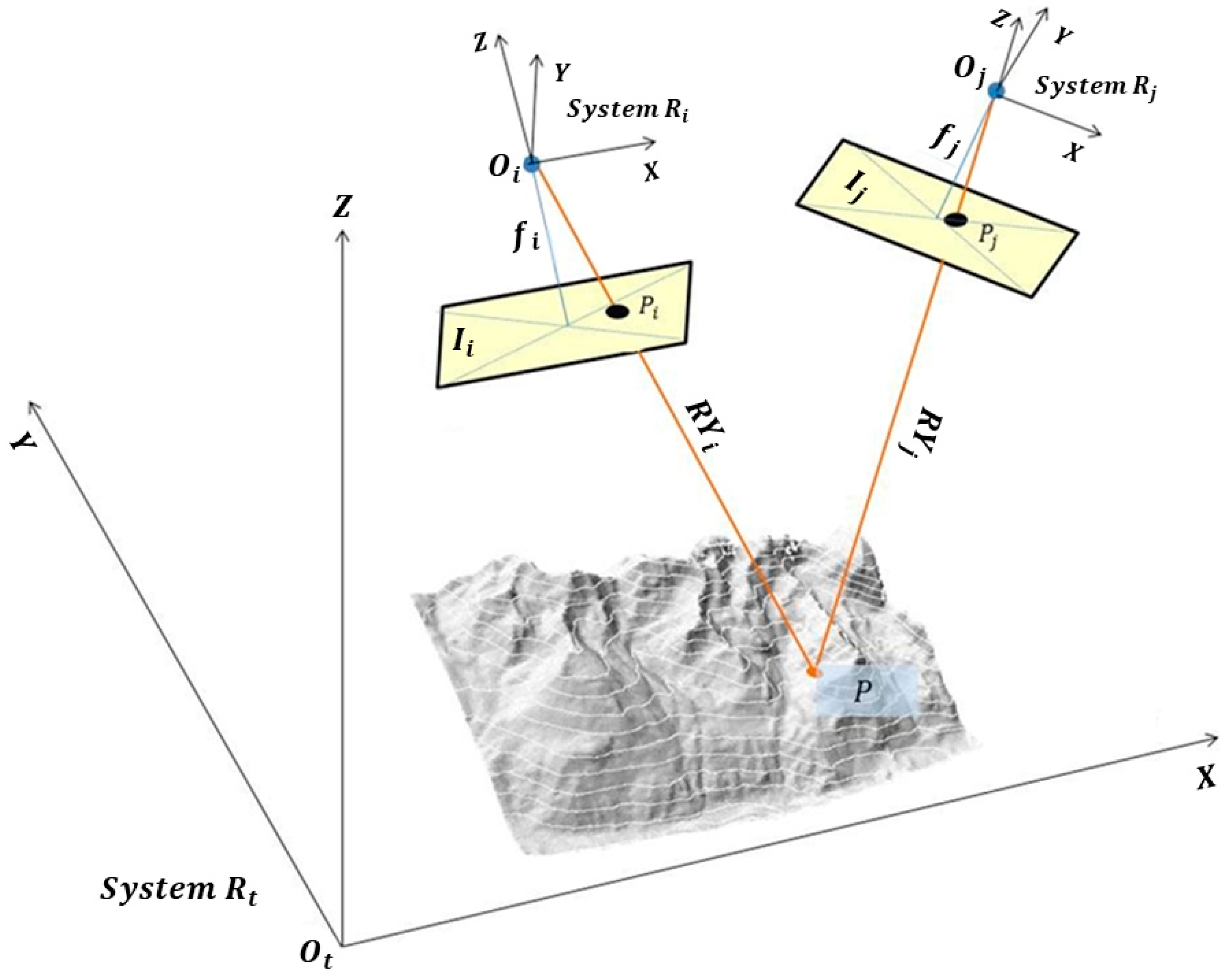
In Figure 4, we define a reference system $R_t$ with a center $O_t$ and one generic terrain point $P$ with coordinates $\left(X_t,Y_t,Z_t\right)$ referring to $R_t$. We created two pictures $\left(I_i, I_j\right)$ of the same place (containing $P$) with two different points of view $O_i: (X_t^{O_i},Y_t^{O_i},Z_t^{O_i})$ and $O_j: (X_t^{O_j},Y_t^{O_j},Z_t^{O_j})$, which refer to $R_t$. The reflection of the rays in $P$ are depicted as the orange lines in Figure 4 ($R{y}_i$ and $R{y}_j$). These lines intersect $I_i and I_j$ in $P_i$ and $P_j$ with coordinates $\left(X_t^i,Y_t^i,Z_t^i\right)$ and $\left(X_t^j,Y_t^j,Z_t^j\right),$ respectively, over the same reference system $R_t$. For all points $P$, the coplanarity condition [7] must be fulfilled ($O_i$, $O_j$, $P_i$, $P_j$ and $P$ are all in the same plane, $\mathsf{\Pi }$) or Equation (3a) must be satisfied.

2.2. Delaunay Triangulation Applied to Digital Elevation Models

One of the most common problems, which will be resolved later on, is the need of LiDAR points in areas where this data is non-existent.

To solve this problem, the density of the LiDAR point cloud is increased by using a Delaunay triangulation [8] using the following process:

• Align a point cloud (denoted as cloud $N_Z$ or cloud $N_I$) over a continuous mathematical surface consisting of flat and triangular elemental surfaces. Among the possibilities that need to be triangulated, there is an ideal solution for the problem we are addressing. This possibility consists of considering the option that ensures all the generated triangles will be as regular as possible and the length of their sides will be at its minimum. This type of triangulation is called “Delaunay triangulation”. The classic Delanuay triangulation can then be characterized as an optimal triangulation that minimizes the interpolation error for isotropic function among all the triangulations with a given set of vertices. For a more general function, a function dependent Delanuay triangulation is then defined to be an optimal triangulation that minimizes the interpolation error for this function and its construction can be obtained by a simple lifting and projection procedure. The Delanuay triangulation of a finite point cloud can be defined by the empty sphere property: no vertices in the point cloud are inside the circumsphere of any simplex in the triangulation. The triangulation formed this way will be unique and the result is a set of triangles with each one defined by three vertices within the points in the cloud [9].
• Obviously, each of these triangles defines a plane in the space that must meet the requirements of Equation (3b), where $\left(X_1, Y_1, Z_1\right)$, $\left(X_2, Y_2, Z_2\right)$ and $\left(X_3, Y_3, Z_3\right)$ denote the coordinates of the vertices of triangles over the reference system $R_t$. Given any (X, Y) inside this triangle, we can calculate its Z (or its I) by interpolation, which enforces the equation of the specified plane. Using this method, we will have increased the density of the initial point cloud and the process can be repeated based on the new points obtained and triangulating once again (see Figure 3):

  $$\left|\begin{array}{ccc}X-X_t& Y-Y_t& Z-Z_t\\ X_t^{O_i}& Y_t^{O_i}& Z_t^{O_i}\\ X_t^{O_j}& Y_t^{O_j}& Z_t^{O_j}\end{array}\right|=0 ,$$

  (3a)

  $$\left|\begin{array}{ccc}X-X_1& Y-Y_1& Z-Z_1\\ X_2& Y_2& Z_2\\ X_3& Y_3& Z_3\end{array}\right|=0.$$

  (3b)

2.3. Equalization of the Digital Images

This project uses grayscale images (false color images can also be displayed). There are two concepts associated with grayscale images, which are the brightness and the contrast.

In order for a digital image to be optimally visualized, it has to be contrasted properly and with a suitable brightness [10]. The synthetic digital images used in this paper are encoded with 8 bits. In other words, the digital values of the pixels must be in the range of 0–255 in order for these images to be displayed on a computer. As the images will be generated by using a specific characteristic of the point cloud (the intensity level in the case of LiDAR), this characteristic can have some values that do not correspond with the levels of 0–255, although they will have to be converted accordingly. This process is known as histogram equalization, which involves each pixel of the image being mapped to a different digital value depending only on its digital value.

The definition of a histogram [11] is given as a graphical representation of a frequency variable presented in the form of bars. In this case, the variable will be the frequency of the pixels according to their intensity within the area defined by the DSM (Digital Surface Model). The contrast of an image provides us with the scatter measurement for the histogram. In other words, a low-contrast image will have a concentrated histogram in the same area. Therefore, the objective will be to equalize the histogram in such a way as to achieve a suitable brightness and contrast, depending on the variable to be represented. To achieve this objective, the mean values are used together with the standard deviation of the variable to be represented (intensity in the case of LiDAR) to find the optimum equalization function.

Given a $N_I$ point cloud and any $i$ point of this cloud, we have:

$$\begin{array}{c}{I}_{inf}=\overline{I}-1.5·{\sigma }_I\\ I_{sup}=\overline{I}+1.5·{\sigma }_I\end{array},$$

(4)

$$\begin{array}{cc}V{D}_i=\frac{255·\left[I_i-I_{inf}\right]}{3·{\sigma }_I}& If I_{inf}\le I_i\le I_{sup}\\ V{D}_i=0 & If I_i\le I_{inf}\\ V{D}_i=255 & If I_i\ge I_{sup}\end{array},$$

(5)

where $\overline{I}$ and ${\sigma }_I$ are the average and the standard deviation of the intensity values in the point cloud; $I_i$ is the value of intensity at point $i$ in the cloud; and $V{D}_i$ is the equalized digital value for this same point $i$.

The selection of this function is not random. Considering that the frequency of repetition of the represented variable follows a normal standard distribution, we guarantee that more than 80% of the values of the variables are to be found within the interval $I_{inf}\le I_i\le I_{sup}$ by taking these indicators.

3. Methodology Development

After the above-explained process, the methodology is further developed following the steps listed below in sequential order:

3.1. Filling the Point Cloud, Calculation of Statistics and Magnitudes

The load of the point cloud will produce a set of $n$ points denoted by $N$ that can be mathematically expressed as:

$$N=\left\{\left(X_0,Y_0,Z_0,I_0\right),\left(X_1,Y_1,Z_1,I_1\right),\dots ,\left(X_t,Y_t,Z_t,I_t\right), \dots ,\left(X_{n-1},Y_{n-1},Z_{n-1},I_{n-1}\right)\right\},$$

(6)

where any point $P_t\in N$ has coordinates $\left(X_t, Y_t, Z_t\right)$ with respect to a system of reference called $R_t$ and with the center in $O_t$. To construct the synthetic images (the intensity level in the case of LiDAR), the attribute $I_t$ will be used.

Once the point cloud has been read, it is used to calculate the following statistics and magnitudes:

$$\begin{array}{c}{X}_{min}=Min\left(X_0,X_1,\dots ,X_{n-1}\right)\\ \\ X_{max}=Max\left(X_0,X_1,\dots ,X_{n-1}\right)\end{array},$$

(7)

$$\begin{array}{c}{Y}_{min}=Min\left(Y_0,Y_1,\dots ,Y_{n-1}\right)\\ \\ Y_{max}=Max\left(Y_0,Y_1,\dots ,Y_{n-1}\right)\end{array},$$

(8)

$$\begin{array}{l}\overline{Z}=\frac{{\sum }_{i=0}^{i=n-1}{Z}_i}{n}\\ {\sigma }_z=\sqrt{\frac{{\sum }_{i=0}^{i=n-1}{\left(Z_i-\overline{Z}\right)}^2}{n}}\\ Z_{min}=Min\left(Z_0,Z_1,\dots ,Z_{n-1}\right)\\ \\ Z_{max}=Max\left(Z_0,Z_1,\dots ,Z_{n-1}\right)\hfill \end{array},$$

(9)

$$\begin{array}{l}\overline{I}=\frac{{\sum }_{i=0}^{i=n-1}{I}_i}{n}\\ {\sigma }_I=\sqrt{\frac{{\sum }_{i=0}^{i=n-1}{\left(I_i-\overline{I}\right)}^2}{n}}\\ I_{min}=Min\left(I_0,I_1,\dots ,I_{n-1}\right)\\ \\ I_{max}=Max\left(I_0,I_1,\dots ,I_{n-1}\right)\end{array},$$

(10)

$$\begin{array}{l}{W}_t=\left(X_{max}-X_{min}\right)\\ H_t=\left(Y_{max}-Y_{min}\right)\\ \delta =\frac{n}{W_t·H_t}\\ S=W_t·H_t\end{array}.$$

(11)

3.2. Calculation of the Initial Parameters

In this second step, the initial parameters needed to generate the synthetic models are calculated:

(a)

The GSD (Ground Sample Distance) is the resolution of the pixel on the ground. The problem is due to the infinite solutions, as, according to the values that we wish to give to the parameters, different images will be obtained. However, only one will be the optimal solution and this is what needs to be found. Given the density of the point cloud $\delta$, calculated according to Equation (11), the best GSD (the GSD with the least magnitude) that can be found is given by the equation:

$$GSD=\frac{1}{\sqrt{\delta }}.$$

(12)

In this way, we have at least one point per pixel. There are other possibilities, but this one is very simple, easy to use and easy to implement.

There are other parameters, which can be fixed according to the data that we already have. Moreover, they can be fixed freely (we have developed the methodology using a model of two frames or images). These parameters include:

(b)

The resolution of pixel $r_p$;

(c)

The focus of the cameras $f_o$ and $f_1;$

(d)

The width and height of the sensor $W_m$ and $H_m$;

(e)

The width and height of the image $W$ and $H$; and

(f)

The flight height $h$.

Once one or more of them have been fixed, the rest are calculated using Equations (13)–(15):

$$\frac{W_m}{f_i}=\frac{W·GSD}{h} \Rightarrow GSD=\frac{W_m·h}{W·f_i},$$

(13)

$$GSD=\frac{r_p·h}{f_i},$$

(14)

$$r_p=\frac{W_m}{W}=\frac{H_m}{H}.$$

(15)

Parameters b–f can be fixed by the operators. It is possible to assign any value to these parameters, but normally all restitution software has tolerances for the size of the digital files, digital camera work with a standard focal length, sensors for cameras have typical dimensions and there is a typical flight height. Therefore, we recommend that typical values are used for all these parameters. Using our own past experience, we first fixed the width and height for pictures to have a standard magnitude (not above 10,000 pixels for width or height), before continuing with focal length and flight length (standard values). Another important advantage of this methodology is that we can work with near 100% overlap. Therefore, most of the pixels in the synthetic images are useful for restitution (Figures 6 and 7). It is very difficult to simulate this situation in real photogrammetry. If one camera is used for all frames, it must be moved from one place to another and if two or more cameras are used at once, the same place must be targeted. Therefore, it is not easy to obtain near 100% overlap in photogrammetry (see Figure 4 where the frames are convergent not orthogonal). In this procedure, we can set the target.

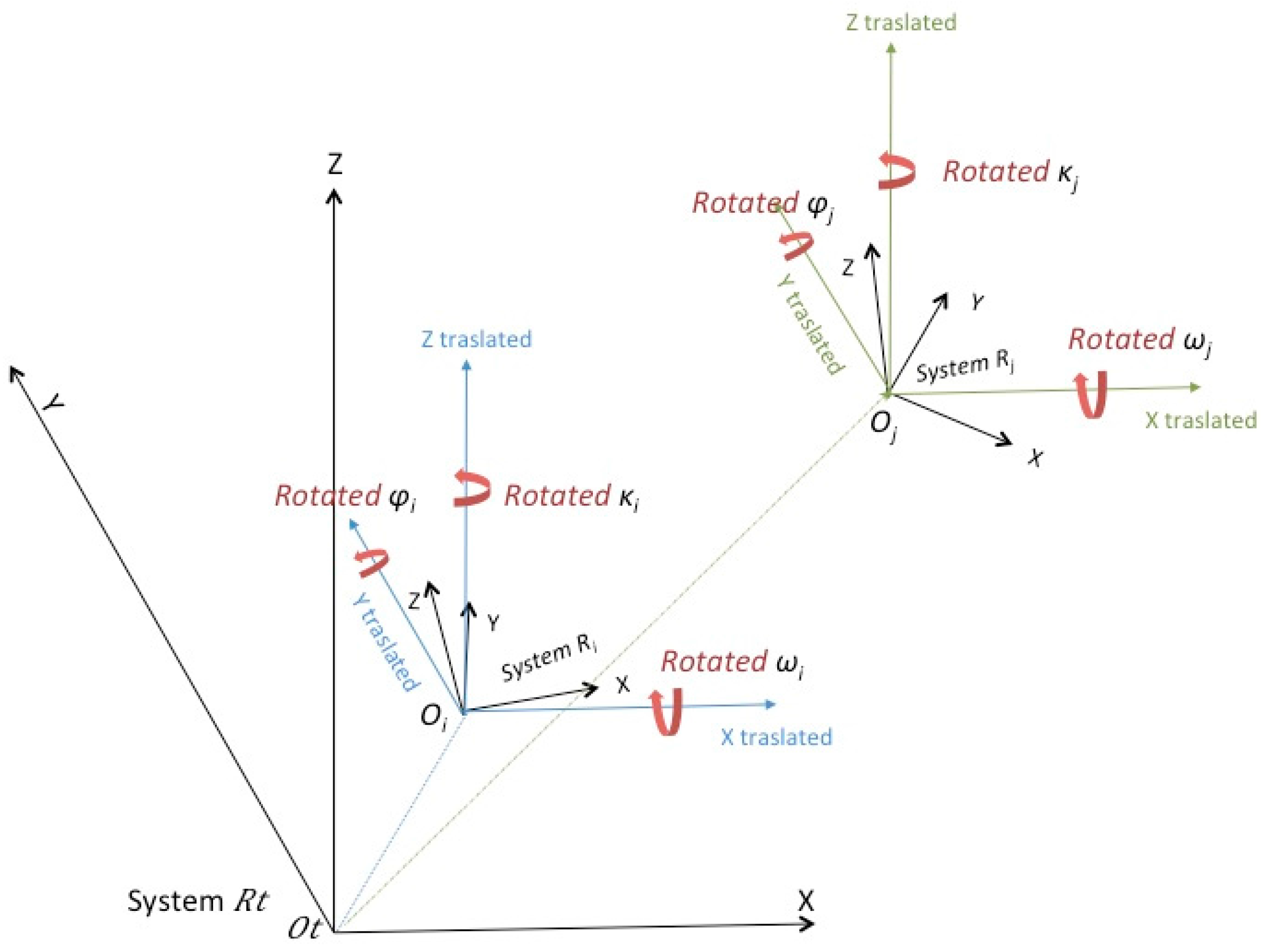
It is possible to introduce (or fix according to all previous magnitudes) the values of the named parameters of the external orientation (Figure 4) for each of the two photographs from which the images $I_0$ and $I_1$ originate. These values are:

(a)

Coordinates of the projection centers $O_0$ and $O_1$ in the systems $R_t$, $\left(X_t{}^{O_o}, Y_t{}^{O_o}, Z_t{}^{O_o}\right)$ and $\left(X_t{}^{O_1}, Y_t{}^{O_1}, Z_t{}^{O_1}\right)$, respectively. A value (in the case that it is not fixed according to our needs) can be fixed according to the coating that is wished for and is called $Re$ (in %) [7,12]:

$$\begin{array}{l}{X}_t{}^{O_o}=X_{min}+\frac{X_{max}-X_{min}}{2}-GSD·W·\frac{100-Re}{200}\\ X_t{}^{O_1}=X_{min}+\frac{X_{max}-X_{min}}{2}+GSD·W·\frac{100-Re}{200}\hfill \\ Y_t{}^{O_o}=Y_t{}^{O_1}=Y_{min}+\frac{Y_{max}-Y_{min}}{2}\hfill \\ Z_t{}^{O_o}=Z_t{}^{O_1}=\overline{Z}+h\hfill \end{array}.$$

(16)

These values are not random. In the best case, the photographs are taken from the center of the area that is being photographed and the flight height $h$ in order to obtain an overlap on the given ground to determine a given perspective between two photographs (separation between the centers of projection) taken orthogonally from the ground.

(b)

Rotations of the cameras ${\omega }_0, {\phi }_0,{\kappa }_0$ and ${\omega }_1, {\phi }_1,{\kappa }_1$ that the photographs, respectively $I_0$ and $I_1$, have been taken with. In the best case, they would all be 0, but an appropriate one can be fixed. It is necessary to establish this value in the case that an overlap near 100% is wanted; thus, this creates convergent photographs instead of orthogonal ones.

3.3. Reading the Point Cloud, Calculating the Pixel Coordinates and Generating Synthetic Pixel

This step is carried out for each point that belongs to the point cloud. The process is laid out in the following sections.

3.3.1. Calculation of the Digital Value of the Pixels to be Represented in Each of the Images $I_0$ and $I_1$

Given a point $P_t\in N$ whose attribute $I$ is $I_t$, the digital value $V{D}_t$ will be in each of the two images given by Equation (17) without having to consider that $V{D}_i=V{D}_t$ and $I_i=I_t$:

$$\begin{array}{cc}V{D}_i=\frac{255·\left[I_i-I_{inf}\right]}{3·{\sigma }_I}& If I_{inf}\le I_i\le I_{sup}\\ V{D}_i=0 & If I_i\le I_{inf}\\ V{D}_i=255 & If I_i\ge I_{sup}\end{array}.$$

(17)

At this point, we have to calculate the equations of the rays denoted by $R{y}_0$ and $R{y}_1.$ Ray $R{y}_0$ passes through points $P_t$ and $O_o$, while ray $R{y}_1$ passes through points $P_t$ and $O_1$. Using Equations (18) and (19), we obtain Equations (20) and (21), which are the equations of lines $R{y}_0$ and $R{y}_1$, respectively:

$$\frac{\left(X-X_t\right)}{X_t-X_t^{O_i}}=\frac{\left(Y-Y_t\right)}{Y_t-Y_t^{O_i}}=\frac{\left(Z-Z_t\right)}{Z_t-Z_t^{O_i}}=l,$$

(18)

$$\frac{\left(X-X_t\right)}{X_t-X_t^{O_j}}=\frac{\left(Y-Y_t\right)}{Y_t-Y_t^{O_j}}=\frac{\left(Z-Z_t\right)}{Z_t-Z_t^{O_j}}=k,$$

(19)

$$\frac{\left(X-X_t\right)}{X_t-X_t^{O_0}}=\frac{\left(Y-Y_t\right)}{Y_t-Y_t^{O_o}}=\frac{\left(Z-Z_t\right)}{Z_t-Z_t^{O_o}}=l,$$

(20)

$$\frac{\left(X-X_t\right)}{X_t-X_t^{O_1}}=\frac{\left(Y-Y_t\right)}{Y_t-Y_t^{O_1}}=\frac{\left(Z-Z_t\right)}{Z_t-Z_t^{O_1}}=k.$$

(21)

The calculation of the equations of the planes denoted by $I_o$ and $I_1$ is shown in Figure 5. In this figure, the plane $I_0$ passes through points $p:\left(0, 0, -f_0\right)$, $p^{\prime }:\left(0, 1, -f_0\right)$ and $p^{″}:\left(1, 0,-f_0\right)$ in the system of reference $R_0$, while the plane $I_1$ passes through points $q:\left(0, 0,-f_1\right)$, $q\prime :\left(0, 1,-f_1\right)$ and $q″:\left(1, 0,-f_1\right)$ in the system of reference $R_1$ (we checked that points $p, p^{\prime }, p^{″}$ and points $q, q^{\prime }, q^{″}$ are not aligned).

Equation (3a) can be applied to planes $I_0$ and $I_1$ to analytically obtain the equations of the planes that refer to the systems of reference $R_0$ and $R_1$, respectively. However, the equations of those planes referring to the system of reference $R_t$ are required. Looking at plane $I_0$ (a similar reasoning as for plane $I_1$) defined by points $p, p^{\prime }, p^{″}$ in the system of reference $R_0$ and applying a spatial transformation of seven parameters (where: $\lambda =1$), the rotations are ${\omega }_0, {\phi }_0, {\kappa }_{0 }$ and the translation is $\left(X_t{}^{O_o}, Y_t{}^{O_o}, Z_t{}^{O_o}\right)$ (Figure 5).

Following this, Equation (22) is applied:

$$\left[\begin{array}{c}Xt\\ Yt\\ Zt\end{array}\right]=\lambda ·R_{\omega ,\phi ,\kappa }·\left[\begin{array}{c}X\\ Y\\ Z\end{array}\right]+ \left[\begin{array}{c}{X}_0\\ Y_0\\ Z_0\end{array}\right],$$

(22)

where $R_{\omega ,\phi ,\kappa }$ is the so-called rotation matrix [13]; $\lambda$ is the scaling factor/custom scale factor; $\left[\begin{array}{c}{X}_0\\ Y_0\\ Z_0\end{array}\right]$ is a vector that shows the translation; and $\left[\begin{array}{c}Xt\\ Yt\\ Zt\end{array}\right]$ are the transformed coordinates of point $P$ of the coordinates $\left[\begin{array}{c}X\\ Y\\ Z\end{array}\right]$ in the initial system.

The result is:

$$\begin{array}{l}\begin{array}{c}\left[\begin{array}{c}X{p}_t\\ Y{p}_t\\ Z{p}_t\end{array}\right]\end{array}=R_{{\omega }_0,{\phi }_0,{\kappa }_0}·\left[\begin{array}{c}0\\ 0\\ -f_0\end{array}\right]+ \left[\begin{array}{c}{X}_t{}^{O_o}\\ Y_t{}^{O_o}\\ Z_t{}^{O_o}\end{array}\right]\\ \left[\begin{array}{c}X{p}_t{}^{\prime }\\ Y{p}_t{}^{\prime }\\ Z{p}_t{}^{\prime }\end{array}\right]=R_{{\omega }_0,{\phi }_0,{\kappa }_0}·\left[\begin{array}{c}0\\ 1\\ -f_0\end{array}\right]+ \left[\begin{array}{c}{X}_t{}^{O_o}\\ Y_t{}^{O_o}\\ Z_t{}^{O_o}\end{array}\right]\\ \left[\begin{array}{c}X{p}_t{}^{″}\\ Y{p}_t{}^{″}\\ Z{p}_t{}^{″}\end{array}\right]=R_{{\omega }_0,{\phi }_0,{\kappa }_0}·\left[\begin{array}{c}1\\ 0\\ -f_0\end{array}\right]+ \left[\begin{array}{c}{X}_t{}^{O_o}\\ Y_t{}^{O_o}\\ Z_t{}^{O_o}\end{array}\right]\end{array},$$

(23)

$$\begin{array}{l}\left[\begin{array}{c}X{q}_t\\ Y{q}_t\\ Z{q}_t\end{array}\right]=R_{{\omega }_1,{\phi }_1,{\kappa }_1}·\left[\begin{array}{c}0\\ 0\\ -f_1\end{array}\right]+ \left[\begin{array}{c}{X}_t{}^{O_1}\\ Y_t{}^{O_1}\\ Z_t{}^{O_1}\end{array}\right]\\ \left[\begin{array}{c}X{q}_t{}^{\prime }\\ Y{q}_t{}^{\prime }\\ Z{q}_t{}^{\prime }\end{array}\right]=R_{{\omega }_1,{\phi }_1,{\kappa }_1}·\left[\begin{array}{c}0\\ 1\\ -f_1\end{array}\right]+ \left[\begin{array}{c}{X}_t{}^{O_1}\\ Y_t{}^{O_1}\\ Z_t{}^{O_1}\end{array}\right]\\ \left[\begin{array}{c}X{q}_t{}^{″}\\ Y{q}_t{}^{″}\\ Z{q}_t{}^{″}\end{array}\right]=R_{{\omega }_1,{\phi }_1,{\kappa }_1}·\left[\begin{array}{c}1\\ 0\\ -f_1\end{array}\right]+ \left[\begin{array}{c}{X}_t{}^{O_1}\\ Y_t{}^{O_1}\\ Z_t{}^{O_1}\end{array}\right]\end{array},$$

(24)

where the equations of planes $I_0$ and $I_1$ are given by the analytical expressions (applying Equation (3)), referring to system $R_t$:

$$\left|\begin{array}{ccc}X-X{p}_t& Y-Y{p}_t& Z-Z{p}_t\\ X{p}_t{}^{\prime }& Y{p}_t{}^{\prime }& Z{p}_t{}^{\prime }\\ X{p}_t{}^{″}& Y{p}_t{}^{″}& Z{p}_t{}^{″}\end{array}\right|=0,$$

(25)

$$\left|\begin{array}{ccc}X-X{q}_t& Y-Y{q}_t& Z-Z{q}_t\\ X{q}_t{}^{\prime }& Y{q}_t{}^{\prime }& Z{q}_t{}^{\prime }\\ X{q}_t{}^{″}& Y{q}_t{}^{″}& Z{q}_t{}^{″}\end{array}\right|=0.$$

(26)

3.3.2. Calculating Coordinates of Points $p_0$ and $p_1$

The coordinates of points $p_0$ and $p_1$ may now be calculated (referring to systems $R_0$ and $R_1$), which are the image coordinates of point $P_t$ of the ground in each image (Figure 4). Once they are transformed to pixel coordinates, the exact position (in column and row) of point $P_t$ of the ground data is generated in each image. This is conducted by calculating the intersection of plane $I_0$ with the line $R{y}_0$ (we already have both references from the same system of coordinates, $R_t$) and ensuring that they also meet the requirements of Equations (27) and (28):

$$\frac{\left(X-X_t\right)}{X_t-X_t^{O_0}}=\frac{\left(Y-Y_t\right)}{Y_t-Y_t^{O_o}}=\frac{\left(Z-Z_t\right)}{Z_t-Z_t^{O_o}}=l,$$

(27)

$$\frac{\left(X-X_t\right)}{X_t-X_t^{O_1}}=\frac{\left(Y-Y_t\right)}{Y_t-Y_t^{O_1}}=\frac{\left(Z-Z_t\right)}{Z_t-Z_t^{O_1}}=k,$$

(28)

$$\left|\begin{array}{ccc}X-X{p}_t& Y-Y{p}_t& Z-Z{p}_t\\ X{p}_t{}^{\prime }& Y{p}_t{}^{\prime }& Z{p}_t{}^{\prime }\\ X{p}_t{}^{″}& Y{p}_t{}^{″}& Z{p}_t{}^{″}\end{array}\right|=0,$$

(29)

$$\begin{array}{l}\left[\begin{array}{c}X{p}_0\\ Y{p}_0\\ Z{p}_0\end{array}\right]=R_{{\omega }_0,{\phi }_0,{\kappa }_0}{}^T·\left\{\left[\begin{array}{c}{X}_t{}^0\\ Y_t{}^0\\ Y_t{}^0\end{array}\right]-\left[\begin{array}{c}{X}_t{}^{O_o}\\ Y_t{}^{O_o}\\ Z_t{}^{O_o}\end{array}\right]\right\}\\ \left[\begin{array}{c}X{p}_1\\ Y{p}_1\\ Z{p}_1\end{array}\right]=R_{{\omega }_1,{\phi }_1,{\kappa }_1}{}^T·\left\{\left[\begin{array}{c}{X}_t{}^1\\ Y_t{}^1\\ Y_t{}^1\end{array}\right]-\left[\begin{array}{c}{X}_t{}^{O_1}\\ Y_t{}^{O_1}\\ Z_{}{}^{O_1}\end{array}\right]\right\}.\end{array}$$

(30)

This intersection will be a point $p_0$ on plane $I_0$ with coordinates (referring to system $R_t$) $p_0:\left(X_t{}^0, Y_t{}^0, Z_t{}^0\right)$. The same procedure will be followed to calculate the intersection of plane $I_1$ with the line $R{y}_1$ (point $p_1$ on plane $I_1$) with the resulting coordinates needing to meet the requirements of both Equations (29) and (30), which means that the coordinates of point $p_1$, referring to system $R_t$, are $p_1:\left(X_t{}^1, Y_t{}^1, Z_t{}^1\right)$. To solve this system, it is advisable to leave just one equation with the parameter l or k, calculate it and then take the coordinates). Now, we have the intersections (points $p_0$ and $p_1$) of Figure 4.

3.3.3. Transformation of Coordinates

After this, the coordinates of these points have to be transformed to the systems of reference $R_0$ and $R_1$. To do this, we use a 3D transformation of seven parameters [13] (three translations, three turns and one scale factor), where Equation (31) is applied to obtain the results after the transformation:

$$\begin{array}{c}{R}_{w_i,{\phi }_i,{\kappa }_i}{}^T=R_{w_i,{\phi }_i,{\kappa }_i}{}^{-1}\\ R_{w_j,{\phi }_j,{\kappa }_j}{}^T=R_{w_j,{\phi }_j,{\kappa }_j}{}^{-1}\end{array}.$$

(31)

3.3.4. Verification of Results

Following this, various checks can be completed to see whether the calculations have been properly compiled. We first checked whether the coordinates $Z{p}_0$ and $Z{p}_1$ from Equation (9) (copied below as Equation (32) for a better reference) should coincide with $-f_0$ and $-f_1$ because these are the points in the planes $I_0$ and $I_1$, respectively:

$$\begin{array}{l}\overline{Z}=\frac{{\sum }_{i=0}^{i=n-1}{Z}_i}{n},\hfill \\ {\sigma }_z=\sqrt{\frac{{\sum }_{i=0}^{i=n-1}{\left(Z_i-\overline{Z}\right)}^2}{n}},\hfill \\ Z_{min}=Min\left(Z_0,Z_1,\dots ,Z_{n-1}\right),\hfill \\ \hfill \\ Z_{max}=Max\left(Z_0,Z_1,\dots ,Z_{n-1}\right).\hfill \end{array}$$

(32)

However, the plane defined by points $P_t{O}_0$ and $O_1$, should contain points $p_0:\left(X_t{}^0, Y_t{}^0, Z_t{}^0\right)$ and $p_1:\left(X_t{}^1, Y_t{}^1, Z_t{}^1\right)$. The intersection on the lines $R{y}_0$ and $R{y}_1$ should be $P_t$.

3.3.5. Transformation of Image Coordinates into Pixel Coordinates

The last step to do is to transform the image coordinates $(X{p}_0, Y{p}_0)$ and the image coordinates $(X{p}_1, Y{p}_1)$ into pixel coordinates. This is conducted based on Equation (33):

$$\begin{array}{c}x=COL·r_p-\frac{W_m}{2},\\ y=\frac{H_m}{2}-\mathit{ROW}·r_p.\end{array}$$

(33)

Following this, Equation (34) is obtained:

$$\begin{array}{l}CO{L}_{I_0}=\frac{X{p}_0+\frac{W_m}{2}}{r_p},\hfill \\ RO{W}_{I_0}=\frac{\frac{H_m}{2}-Y{p}_0,}{r_p}\hfill \end{array}$$

(34)

$$\begin{array}{l}CO{L}_{I_1}=\frac{X{p}_1+\frac{W_m}{2}}{r_p}\hfill \\ RO{W}_{I_1}=\frac{\frac{H_m}{2}-Y{p}_1}{r_p}\hfill \end{array}.$$

(35)

Finally, the digital value $V{D}_t$, which was previously calculated, is assigned to each of these pixels in both images.

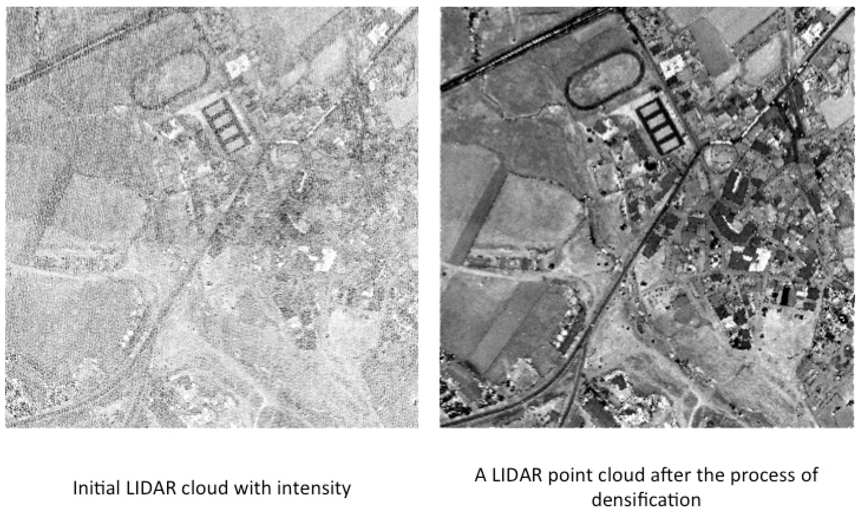
3.4. Densifying Point Cloud

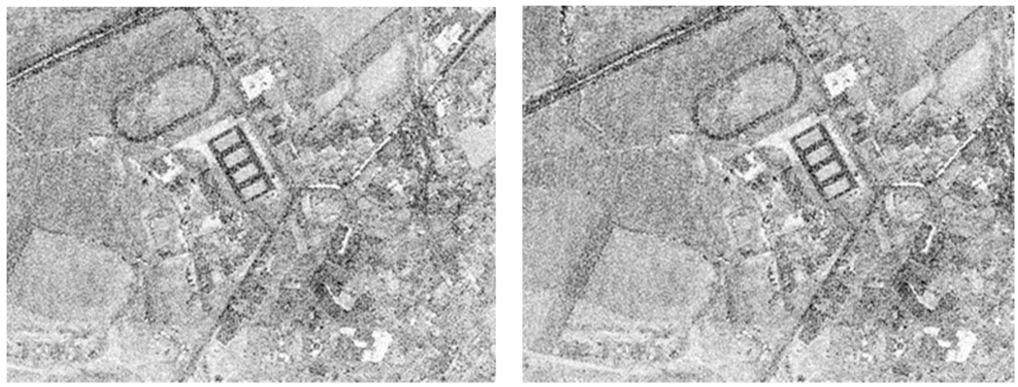
When Step 3 is applied to all points of the cloud, a photogrammetric model is generated. The generated images will be similar to pictures shown in Figure 6.

In Figure 6, we can see that there is an insufficient number points to visualize the images in the digital photogrammetric station using photogrammetric software. This obvious lack of quality is due to the fact that the point cloud used is not a regular mesh. In other words, the density of points per square meter is not constant throughout the cloud and the points are not well-distributed. There are points on the ground that correspond to the same pixel in the images despite having different intensity levels. In this case, we discard all except one and we consider this digital value as the mean value of intensity level.

To resolve this issue and to obtain a well-distributed and uniform cloud of points, we could use a “nearest neighbor” type of algorithm in both images. With this algorithm, we could fill the areas with no points and we could create new points using the intensity level of neighbors. In our case, this is impossible because we would lose 3D vision as it would become noise in the digital image. The reason for this can be easily understood by analyzing Figure 4. If we create a new point $P_0^h$ in $I_o$ using the nearest neighbor algorithm, the next stage would be to find this point ($P_1^h$) in image $I_1$ and assign the same digital value to it. However, this is not possible because we do not know the position of $P_0^h$ in the terrain, so that it is impossible for us to find the homologous point in $I_1$ and 3D vision requires the same point in both images ($P_0^h$ and $P_1^h$) The reconstruction of ray $R{y}_1$ is not available and, therefore, point $P_1^h$ cannot be obtained.

The solution for this issue is to densify the initial point cloud $N$ by adding new points as follows:

-

First of all, we must find all these zones so we used the software to automatically find all pixels with no value in both synthetic images (left and right).

-

We selected a zone with no points in the left image called $H_0$ with $k$ neighbor pixels in this image (once we complete the process with the left image, we apply the same process to the right image) with pixel coordinates $\left(CO{L}_k, RO{W}_k\right)$ and intensity level $I{L}_k.$ Following this, we obtained the ground coordinates $\left(X_k,Y_k, Z_k\right)$ for all $k$ points, which are previously calculated in the process of generating the synthetic image as there is one unique correspondence between all points in the cloud, all points in image $I_o$ and all points in image $I_1$. Following this, we created a new point $P_h$ (in the center of all $k$ points) with ground coordinates $\left(X_h,Y_h,Z_h\right)$ and intensity level $I{L}_h$, using the mean intensity level of all $k$ points for digital value of intensity. After this, we have the new point $P_h$, and, then, we can obtain pixel coordinates in both images $I_0$ and $I_1.$ We repeated this process as many times as necessary to get a well-distributed point cloud. The point cloud $N$ has a new point called $P_h$ and the synthetic images are generated again with the initial point cloud in addition to the set of interpolated points created. Obviously, the holes are filled in both images.

The result obtained after completing this process in the images is shown in Figure 7. As you can see, the images of Figure 7 appear to be denser compared to the images of Figure 6.

4. Quality Control

Quality is defined as the “property inherent in anything that allows it to be compared with anything else of the same species or nature” [14]. For this purpose, certain procedures and controls have to be provided to guarantee the integrity, accuracy and entirety of the data. In other words, it is necessary to verify that the desired quality has been reached [14].

In the case of the information provided by the photogrammetric method, these are the classic aspects [15] related to redundancy measures. The results of the photogrammetric triangulation provide the quantitative measurements for the precision of the results:

-

Variance of the components;

-

Variance–covariance of the coordinates of the calculated objects;

-

Comparison of values with nominal data;

-

Independent measurements to verify the precision via a point control analysis; and

-

Comparison of coordinates of the photogrammetric points with the independently obtained coordinates (i.e., GPS in the field).

With regards to the LiDAR information, the control is a secondary procedure to ensure and verify the quality of the registered data. It can be conducted in terms of two criteria:

• “Causes”: study the behavior of the elements that define the mathematical model of adjustment, where we consider both “internal causes” (flight plan: external orientation and calibration) and “external causes” (flight conditions: direction of the flight paths, flight height, etc.) as well as ground type (altitude, type of vegetation, etc.).
• “Effects”: the results given by the point cloud and where the following has to be taken into consideration: the “relative internal effects” (topographical control and planimetric control) and “relative external effects” (control points, difference between Digital Terrain Model and DSM, differing intensity levels and stereoscopic checking). In most cases, the quality control of the results is conducted starting with this second criterion, while the possible corrections of the results are completed using the elements of the equations chosen for the adjustment.

In our case of study, we performed three tests to estimate the quality of the results obtained (a test zone in the city of Alicante, Spain) with the software developed. First, a planimetric control was used (only to estimate accuracy for X and Y coordinates). In this case, we compared a picture obtained with classical photogrammetry PNOA (Plan Nacional de Ortofotografía Aérea) [16] with a synthetic picture generated for the same place using our methodology (we describe this procedure in planimetric analysis, Section 4.1). The PNOA picture has the best accuracy so this is used as reference. For the second test (to estimate accuracy for Z-coordinate, described in Section 4.2 as 3D analysis), we used a similar procedure to compare two digital models. The first digital model was obtained from classical photogrammetric pictures, while the second one was obtained from synthetic pictures (both in the same area, Alicante, Spain). Finally, we compared these two images with X-, Y- and Z-coordinates using a 3D transformation. In order to compare all these data and to measure the quality, we have used the software developed within the framework of a previous study [14].

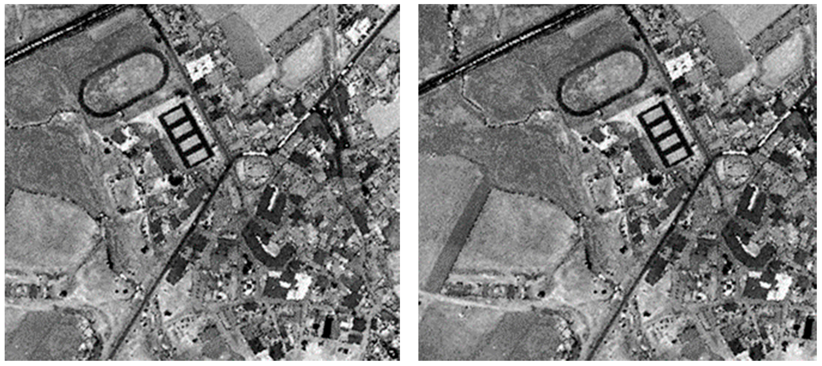
4.1. Planimetric Analysis

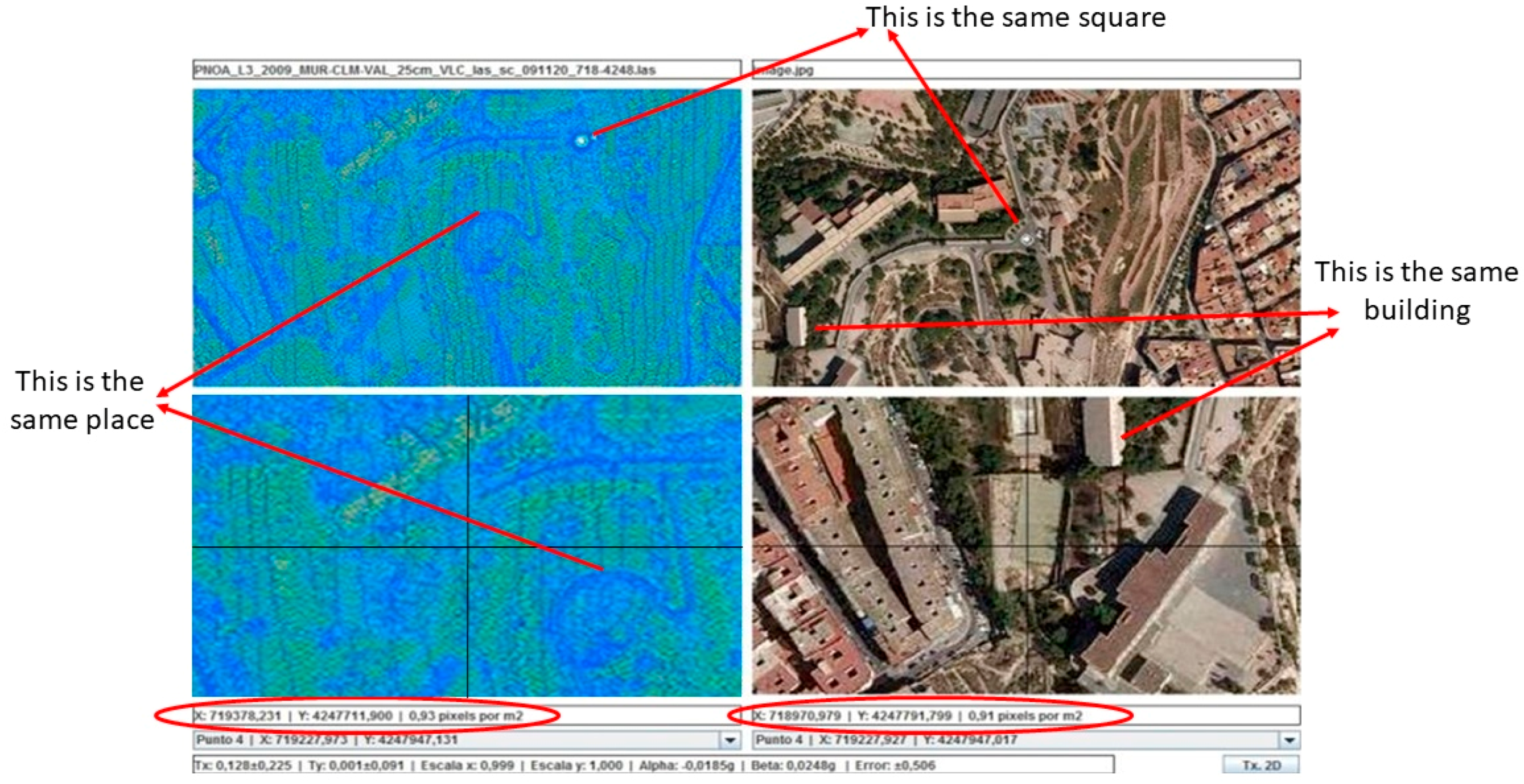
In this case, we are interested in obtaining planimetric precisions. We compared two images (see Figure 8) with the PNOA picture being used as a reference (right side in Figure 8), while the another one was obtained using a synthetic procedure (left side in Figure 8, using a blue color ramp) for a test zone (2 × 2 km) in the city of Alicante ($X_{min}=\mathrm{720,000} \mathrm{m}; X_{max}=\mathrm{722,000} \mathrm{m}; Y_{min}=\mathrm{4,246,000} \mathrm{m}; Y_{max}=\mathrm{4,248,000} \mathrm{m}$, UTM 30N datum WGS84). Note that $X_{min}$, $X_{max}$, $Y_{min}$ and $Y_{max}$ refer to test area, so the pictures shown in Figure 8 cover more territory. A good way to compare these two images is to use a 2D transformation [17] by selecting at least three of the same points in both images to obtain six parameters for affine transformation (T_x, T_y, S_x, S_y, α and β). In the example of Figure 8, the operator selected the same four points for both pictures and using the method of least squares [18], we obtained the following values for the six parameters (two translations, T_x and T_y; two scale factors S_x and S_y; one rotation α and one perpendicularity β):

$$\begin{array}{l}{T}_x=0.128 \mathrm{m}\hfill \\ T_y=0.001 \mathrm{m}\hfill \\ S_x=0.999\hfill \\ S_y=1.000\hfill \\ \alpha =-{0.0185}^g\hfill \\ \beta ={0.0248}^g\hfill \end{array}.$$

(36)

There is a mean squared error of $\pm 0.506 \mathrm{m}$ for the adjustment. This estimated error is below the GSD used in generating the synthetic images (1 m).

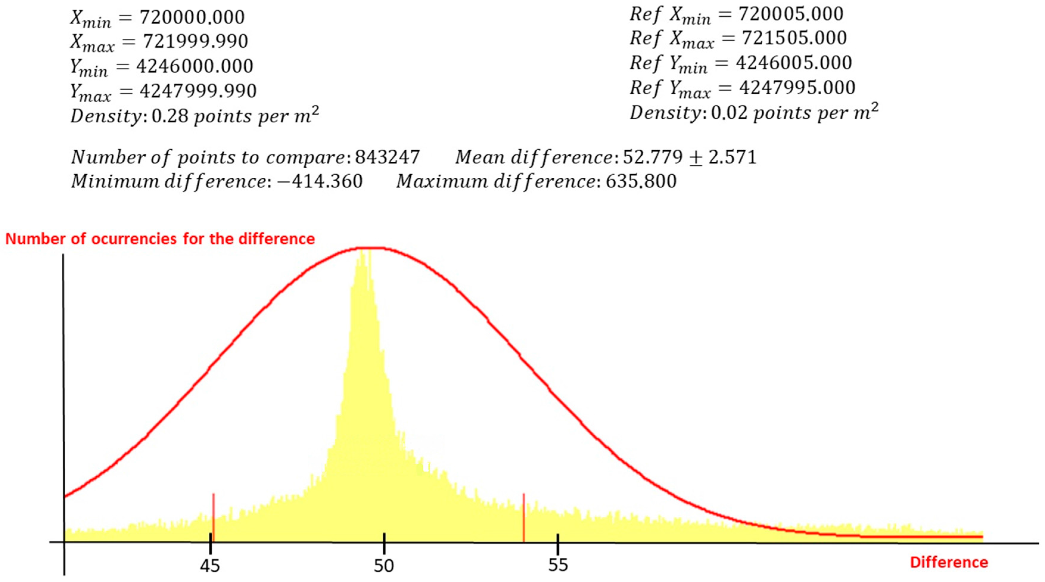
4.2. 3D Analysis

We will estimate the accuracy for the Z-coordinate in this section. In this case, we compared the calculated DEM obtained with the synthetic images with a reference one that has better precision [16] used as a reference. After that, both models were superimposed and compared in the same area of Alicante ($X_{min}=\mathrm{720,000} \mathrm{m}; X_{max}=\mathrm{722,000} \mathrm{m}; Y_{min}=\mathrm{4,246,000} \mathrm{m}; Y_{max}=\mathrm{4,248,000} \mathrm{m}$, UTM 30N datum WGS84) to obtain the difference in a total of 843,247 points. This is seen in the histogram of Figure 9, which represents the difference in Z-coordinate between the two models (X-axis represents the difference in meters and Y-axis represents the number of times that this difference occurs). From this analysis, we obtained a mean difference of $52.779\pm 2.671 \mathrm{m}$ between the two models. In a first analysis, this difference is huge, but it is necessary to remember that one digital model (PNOA used as reference) has orthometric heights and the other one (synthetic) has ellipsoidal heights. In Alicante, the geoid height above the ellipsoid is over 50 m [19].

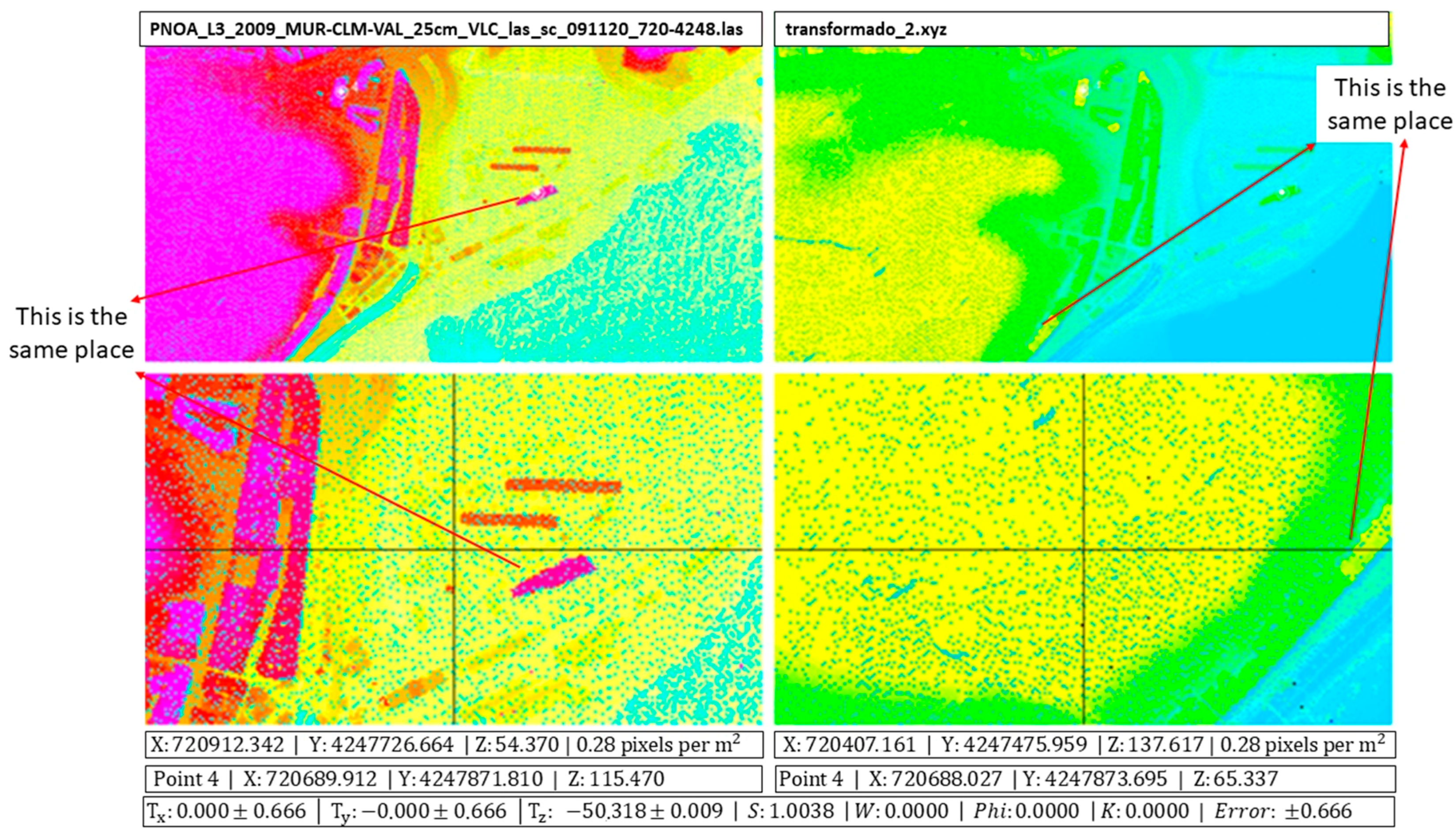
4.3. Plani-Altimetric Analysis

The tool provided by the software allows the calculation of the spatial transformation [20] between two images with Z-coordinates. Using this transformation, we can evaluate the errors for the X-, Y- and Z-coordinates. The Helmert 3D transformation provides us with three translations (T_x, T_y and T_z), one scale factor (S) and three rotations (ω, φ and ϰ). In this case, we compared two raster files with the Z-coordinates, with one having better precision (right side in Figure 10) and the other obtained using the synthetic procedure (left side in Figure 10). A color ramp was used in both cases. The operator selects a minimum of three well-distributed points (the same for two images) to obtain these parameters:

$$\begin{array}{l}{\mathit{T}}_{\mathit{x}}=\mathbf{0.000} \mathbf{m}\hfill \\ {\mathit{T}}_{\mathit{y}}=\mathbf{0.000} \mathbf{m}\hfill \\ {\mathit{T}}_{\mathit{z}}=\mathbf{50.318} \mathbf{m}\hfill \\ \mathit{S}=\mathbf{1.004}\hfill \\ \mathbf{\omega }={\mathbf{0.0000}}^{\mathit{g}}\hfill \\ \mathbf{\phi }={\mathbf{0.0000}}^{\mathit{g}}\hfill \\ \mathbf{\aleph }={\mathbf{0.0000}}^{\mathit{g}}\hfill \end{array}.$$

(37)

There is a mean squared error of $\pm 0.666 \mathrm{m}$ for the adjustment. Figure 10 shows that there is a displacement in the Z-coordinate (the geoid height above the ellipsoid for Alicante). We can see that the rotations are 0 and the scale factor is 1.004.

5. Conclusions

The main goal of this work is to provide an easy and cheap alternative technique to visualize point clouds using photogrammetric software and digital restitution stations. This will be extremely useful in cases where the use of photogrammetry may not be an option due to high costs, adverse weather and so on.

5.1. Comparison with a Classic Photogrammetric Flight

In classic photogrammetry, the hypsometric error ${\sigma }_h$ (which is what determines the overall accuracy where the Z-axis contains the direction of the optical axis) is expressed as:

$$\begin{array}{c}{\sigma }_h={\sigma }_p·\frac{h}{f}·\frac{h}{b}\\ {\sigma }_p=\frac{\sqrt{2}}{2}·r_p\end{array},$$

(38)

where ${\sigma }_p$ is the planimetric error in the instrument; $h$ is the flight height; $f$ is the focus of the camera; $r_p$ is the pixel resolution (squared in our example) and $b$ is the base area. In the equation, $\frac{h}{f}$ is defined as the flight scale $E_v$.

The prototype has a GSD of 1 m, a focus of 50 mm, a pixel resolution of 50 microns, a flight height of 1 m and a base area of 165 m. With this data, $E_v$ is 1:20,000, ${\sigma }_p$ is 35 microns and ${\sigma }_h$ = ±4 m, which gives an equidistance in the curve level of 10 m. Therefore, a minimum scale for the cartography is obtained as 1:10,000, which reinforces the consistency of the model. A GSD of 1 m marks a cartography scale of 1:5000.

5.2. Uses of LiDARgrammetry

The mere act of carrying out a LiDAR flight or a Laser Scanner survey does not mean we have to take photogrammetric shots in order to carry out classic photogrammetric restitution. By applying the methodology developed in this approach, stereoscopic models that are returned using a modern photogrammetric station scan can be generated. This can be an added advantage in cases where it is impossible to obtain images (night flights, clouds, radar images, sea beds and so on).

5.3. Quality Control Tools

These techniques can also be used to see whether the cartography obtained with classic photogrammetry is sufficiently accurate. This evaluation involves first generating the synthetic photogrammetric models of an area surveyed with LiDAR and collecting the results obtained using traditional photogrammetric techniques in this area. Following this, a comparison will show the accuracy of the original cartography.

5.4. Help with Classification and Filtering

The generation of synthetic images can help with the editing of LiDAR point clouds, as it allows us to carry out a process prior to classification and filtering.