
Inverse Optimal Design for Position Control of a Quadrotor

1
School of Electrical and Electronic Engineering, Yonsei University, Seodaemun-Gu, Seoul 03722, Korea
2
Department of Electronic Engineering, Kyonggi University, Suwon, Kyonggi-Do 16227, Korea
*
Author to whom correspondence should be addressed.
Appl. Sci. 2017, 7(9), 907; https://doi.org/10.3390/app7090907
Submission received: 18 June 2017
/
Revised: 11 August 2017
/
Accepted: 26 August 2017
/
Published: 5 September 2017
Abstract
:In this paper, we propose an inverse optimal design method for the position control of a quadrotor. First, we derive the dynamics of a quadrotor using the Newton-Euler formulation. Second, we present the state transformation technique to derive the position dynamics from the kinematic and dynamic models of a quadrotor. Then, we present the nonlinear inverse optimal position control of a quadrotor. The stability analysis based on Lyapunov theorem shows that the proposed control method can realize a quadrotor system that is exponentially stabilized. In addition, we show the inverse optimality of the proposed inverse optimal controller for the position control of a quadrotor. The inverse optimality can simply and clearly be shown using the state transformation technique. Finally, we present some simulation results to verify the effectiveness of the proposed control method.
1. Introduction
Over the past few years, the field of unmanned aerial vehicles (UAVs) has rapidly expanded. In addition, because of the advantage of UAVs, there has been an increase in their applications, such as aerial reconnaissance, where life-saving operations are risky for pilots, and disaster surveillance and monitoring. In particular the quadrotor, one type of UAV, has many advantages. It has the advantage of easy implementation compared to other aerial vehicles. In addition, it has vertical take-off and landing (VTOL) ability, high agility and maneuverability.
Recently, there has been significant interest in the application of quadrotors, so there has been much attention on the studies that focus on the control of a quadrotor. In the field of a quadrotors, the problem of control design has focused primarily on typical quadrotor missions including attitude stabilization and movement from one position to another position. Linear control methods such as proportional-integral-differential (PID) control and the linear quadratic regulation (LQR) control methods are proposed in [1,2]. However, linear control methods simplify the model and focus only on the local behavior of the system.
In practice, quadrotors have complicated dynamics with coupled states that cause nonlinearities. Furthermore, the dynamics of a quadrotor are not only nonlinear, but they are also difficult to characterize because of the complexity of the aerodynamic properties.
For these reasons, various nonlinear control methods have been proposed including nested saturations [3], dynamic inversion control approach [4], sliding mode control methods [5,6], feedback linearization method [7], backstepping control approaches [8,9,10], integral predictive nonlinear control [11], and neural network based output feedback control method [12]. Meanwhile, using optimal control techniques, research for battery operation and missions to consider the optimality have been performed [13,14]. In other words, researchers are interested in realizing the optimality of controllers other than the stability.
The optimal control problem for nonlinear systems is usually attributed to the solvability of the Hamilton-Jacobi-Bellman (HJB) equation. Because the HJB equation involves partial differential equations, optimal control design is generally too difficult to be solved analytically, with the exception of a few special cases. An alternative method is the so-called inverse optimal control method, which does not require a solution to the HJB equation [15]. In this case, the minimization of the performance index is determined a posteriori according to the given controller, so the aforementioned difficulty can be alleviated.
In [16], the author proposed an inverse optimal control of a quadrotor by employing the backstepping technique. However, it involves controlling only the attitude of a quadrotor. Moreover, to the best of the authors’ knowledge, there have been no reports on the application of inverse optimal based position control for quadrotor systems.
Most of the research into the position control of quadrotors use the small-angle assumption to simplify the position of the dynamic equation of a quadrotor [1,3,17], and they derive the reference roll and pitch angles that are outputs from the position controller. Unlike the aforementioned methods, in this paper, we derive the reference roll and pitch angle caused by the modified dynamics of the position of a quadrotor using the state transformation technique without any assumption. Furthermore, we employed the state transformation technique to simplify the design process of the inverse optimal controller. In addition, it can make the proof of inverse optimality simple.
In this paper, we propose an inverse optimal position control of a quadrotor. First, we derive the dynamics of the quadrotor using the Newton-Euler formulation. Then, we present the state transformation technique to derive the position dynamics from the kinematic and dynamic models of a quadrotor. Our proposed design of the nonlinear inverse optimal position control of a quadrotor is based on the work in [18], where Movric and Lewis suggest the algebraic Riccati equation (ARE)-based inverse optimal controller design for general time-invariant systems. The stability analysis based on Lyapunov theorem shows that the proposed control method result in a quadrotor system that is exponentially stabilized. Further, we show the inverse optimality of the proposed inverse optimal controller for the position control of a quadrotor. The inverse optimality can simply and clearly be shown using the state transformation technique. Finally, we perform simulations to verify the effectiveness of the proposed method.
The remainder of the paper is as follows: In Section 2, we describe the dynamics of the quadrotor, which is derived using the Newton-Euler formulation. In Section 3, we propose an altitude controller based on inverse optimal position control method. We show the stability and inverse optimality of the proposed inverse optimal controller for the position control of a quadrotor. In Section 4, we present the simulation results, and conclude the paper in Section 5.
2. Dynamic Model of a Quadrotor
A quadrotor has a cross configuration with four motors, each of which is attached to each end of a cross-shaped body. The four motors are equipped with propellers whose axes of rotation are all parallel to each other. The behavior of a quadrotor can be controlled by adjusting the rotational velocities of these four propellers. The equations describing the position and attitude motions of a quadrotor are those of a rotating rigid body with six degrees-of-freedom (DoFs).
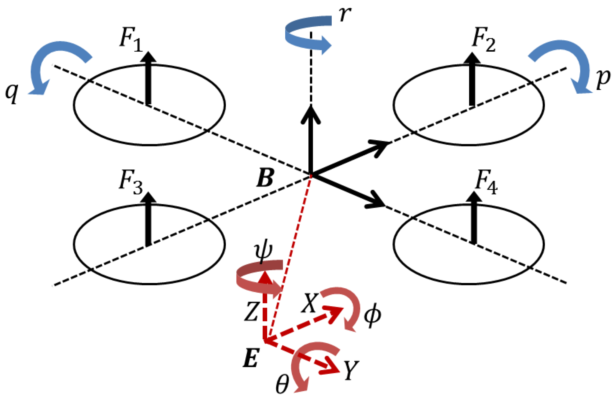
To derive the equation for the movement of a quadrotor, we should to consider the coordinates of a quadrotor system. The generalized coordinates of a quadrotor system is shown in Figure 1, where B and E denote the body-fixed and earth inertial frames, respectively.
Let us assume that the generalized velocity vectors with respect to the earth inertial and body-fixed frames are in the form of and , respectively. Here, represents the position of the center of mass of a quadrotor and are the Euler angles representing the orientation of a quadrotor, namely roll-pitch-yaw, with respect to the earth inertial frame. Similarly, and represents the linear and angular velocity of the quadrotor with respect to the body-fixed frame, respectively.
Now, we describe the kinematics of a generic six-DoF rigid-body as follows:
where, is a 3 by 3 submatrix filled with all zeros, R is the coordinate transformation matrix from the body-fixed frame to the earth inertial frame, and T is the angle-rates transformation matrix from the body-fixed frame to the earth-inertial frame. Here, matrices R and T are defined, respectively, as follows:
where , , and .
To describe the dynamic model of the position of a quadrotor, we use the Newton-Euler formalism. The dynamics of a generic six-DoF rigid-body takes into account the mass of the body. The dynamics of the position is described by
where m is the mass of a quadrotor, refers to a 3 by 3 identity matrix, is the linear velocity vector, is the linear acceleration vector of the body-fixed frame, is the angular velocity vector of the body-fixed frame, and is the force vector of the body-fixed frame. However, it may be useful to express the dynamics of the position using the earth-inertial frame.
The nonlinear dynamics of a quadrotor can be described by
where g is the gravitational acceleration, and is the attitude control input represented by
Here, is the propeller speed of the i-th rotor and b is the thrust factor of a quadrotor.
3. Design of Inverse Optimal Position Controller
In this section, we design an inverse optimal position controller to converge the position states of a quadrotor to the reference values.
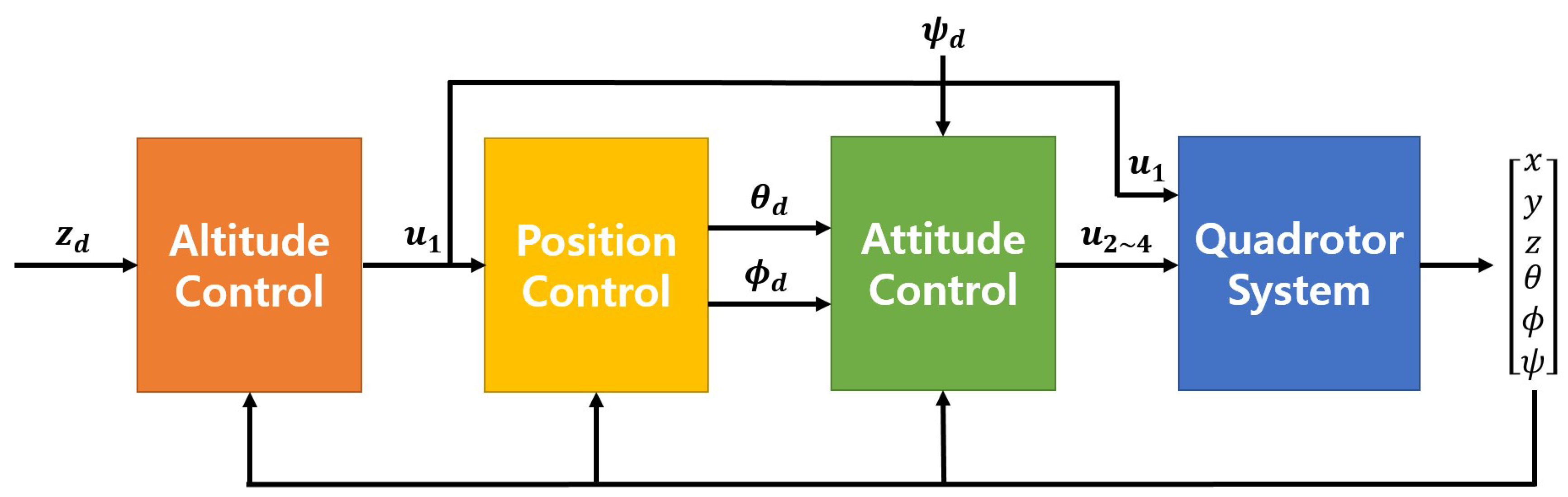
For the position control, inverse optimal based altitude controller is designed. Next, the reference roll and pitch angles are calculated through altitude control based position control. Finally, the position control of the quadrotor is performed through attitude tracking control. The overall control scheme is expressed by the block diagram as Figure 2.
In (5), the () positions dynamics of a quadrotor can be represented, using the states and , as follows:
where , and .
Using the redefined control input U and the input-coupling transformation matrix , which is invertible, (7) can be rewritten as follows:
We analyze the position control problems of a quadrotor from two perspectives. The first one is the exponential stability, while the other one is the inverse optimality.
The position of a quadrotor converges to the reference position. In other words, the position state P of a quadrotor satisfies the following equation related to the position control of a quadrotor:
where and are the initial and reference positions, respectively.
In this paper, we also show the inverse optimality of the proposed control input. The control input U, which makes the position error zero, minimizes the following objective functional:
for a positive definite matrix and . Here, the position error is defined as .
Using the position dynamics of a quadrotor, as expressed in (5), we can find the altitude control input of a quadrotor, which is presented as the dynamics of its () position. In this paper, using the characteristics of the position dynamics, as explained above, we design the () position control input using the altitude control input .
In this paper, to design an inverse optimal position controller, we use the following assumption:
Assumption 1.
In the control system, the position and attitude values of the quadrotor can be perfectly estimated.
3.1. Altitude Control of a Quadrotor
In this paper, we propose an altitude control input based on the inverse optimal position control method. To do this, the altitude dynamics in (5) can be rewritten in state-space form using the following states:
We have the altitude state-space equation of a quadrotor as follows:
where is the pseudo altitude control input defined by
and is the first transformation variable given by
The states and related to the altitude of a quadrotor can be rewritten by the state , as follows:
where is the reference value of the altitude.
Differentiating with respect to time, we obtain
where and are defined as and , respectively.
For the invertibility of , throughout the paper, we use the following assumption.
Assumption 2.
The attitude angles , θ, and ψ satisfy the following conditions:
The parameters, and are function of time, so we can express (15) as (16):
where we denote with a slight abuse of notation.
For the system (16), we propose the following inverse optimal pseudo altitude control input of a quadrotor:
where is given by
where we denote with a slight abuse of notation.
Here, the is given by
and is the solution of the ARE
where , , and a positive definite matrix , , respectively.
Therefore, based on the definition of in (17) and (11), we can derive the actual altitude control input as follows:
Theorem 1.
Consider the transformation variable , as shown in (13), and the altitude system (16) of a quadrotor using the pseudo altitude control input (17). Then,
(i) Stability: The pseudo altitude control input (17) asymptotically stabilizes the altitude system (16) of a quadrotor. In addition, the state in (14) decreases exponentially with regard to the initial value, i.e.,
with positive constants α and κ.
(ii) Inverse Optimality: The pseudo altitude control input (17) of a quadrotor minimizes the objective functional
for a positive definite matrix and the .
Proof of Theorem 1.
(i) Stability: Substituting (17) into (16), we obtain the altitude system (16) of a quadrotor as follows:
Consider the positive definite function = as a Lyapunov function candidate. Differentiating with respect to the time and substituting (23), we obtain
Since is a symmetric matrix satisfying , we obtain
Therefore, we have , which implies the exponential stability of the system. When the time becomes infinity, the state related to the altitude of a quadrotor becomes zero.
(ii) Inverse Optimality: In order to prove the inverse optimality, we use the comparison Lemma [19]. Then, we have
Therefore, we can check that has a finite value. In addition, using (17)–(19), can be rewritten as follows:
From the definition of , we can show that is satisfied. Therefore, integrating (24) with respect to time from zero to infinity, we have
Because and are positive definite matrices, the matrices , , , , and satisfy the matrix-type HJB equation
Then, is the optimal solution for the objective functional (25).
Remark 1.
Remark 2.
For the following objective functional J subject to system (16), and the given attitude trajectory and , the input is the optimal solution to minimize the following objective functional J.
The is the solution of the ARE (20), and it is the convergence value of the solution of the following differential Riccati equation when goes to infinity.
This is equivalent to the optimal solution of matrix-type HJB (26) mentioned in the proof of this paper.
This Remark applies in a similar way to the () position control in the next Section 3.2. Therefore, the Remark is omitted in the position control in Section 3.2.
3.2. Position Control of a Quadrotor Based on Altitude Control
In this section, to realize the position control of a quadrotor, we define the variable , using the actual altitude control input , as follows:
To design the position control of a quadrotor, the dynamics of a quadrotor (5) can be rewritten in state-space form using the following states:
We obtain the () position state-space equations of a quadrotor as follows:
Rearranging these equations, we finally obtain the following position dynamics (7) of a quadrotor as follows:
where P and V are defined as and , respectively, and are the effective control inputs are defined by
To express (32) in a form like that of (8), substituting the altitude input (30) of a quadrotor into the position dynamics (32) of a quadrotor and using the transformation matrix given by
we obtain the matrix-type position dynamics of a quadrotor as follows:
where and .
The states P and V, which are related to the position of a quadrotor, can be rewritten as the state , as follows:
where is the reference value of the position, is the reference velocity value along the X and Y axes.
Differentiating with respect to time, we have
where and are defined as and , respectively, and .
The parameters, , , , and are function of time, so we can express (37) as follows:
where we denote with a slight abuse of notation.
For the system (38), we also propose the following inverse optimal () position control input of a quadrotor:
where is given by
where we denote with a slight abuse of notation.
Here, a positive definite matrix is given by
and is the solution of the ARE
where and , respectively, and a positive definite matrix , are the positive matrices.
Through the () position dynamics (35) of a quadrotor, which is expressed in terms of P, V, and given by (34), we can consider the position control input defined by
Assumption 3.
To derive a reference attitude value for position control, the attitude of the quadrotor is assumed to be perfect tracking.
The motion along the x and y axes is related to the pitch and roll angles, respectively. The reference roll() and pitch() angles of a quadrotor that enable the quadrotor to converge in the desired position are obtained from the inverse optimal position control input designed in Section 3.2. Therefore, the reference roll() and pitch() angles are obtained by using the position control input (42) as follows:
For notational convenience, we will use the state vector throughout the following lemma and theorem that gives the stability and inverse optimality of the position control input (39).
Lemma 1.
Theorem 2.
Consider the transformation matrix , as shown in (34) satisfying Lemma 1, and the () position system (38) of a quadrotor with the position control input (39). Then,
(i) Stability: The position control input (39) asymptotically stabilize the () position system (38) of a quadrotor. Further, the state in (36) decreases exponentially with regard to the initial value, i.e.,
with positive constants α and κ.
(ii) Inverse Optimality: The () position control input (39) of a quadrotor minimizes the objective functional
for some positive definite matrix and a time varying positive definite matrix .
Proof of Theorem 2.
From Lemma 1, (45) can be rewritten as
Consider the positive definite function = as a Lyapunov function candidate. Differentiating with respect to the time and substituting (45), we obtain
Since is a symmetric matrix satisfying the equation , we obtain
Therefore, we have , which implies the exponential stability of the system. When the time goes to infinity, the state related to the () position of a quadrotor goes to zero. Therefore this result solves the position control problem (9).
(ii) Inverse Optimality: In order to prove the inverse optimality, we use the comparison Lemma [19]. Then, we have
Therefore, we can check that has a finite value. In addition, using (39) and (40), can be rewritten as
From the definition of , we know that is satisfied. Therefore, integrating (47) with respect to time from zero to infinity, we obtain
Because and are positive definite matrices, matrices , , , , and satisfy the matrix-type HJB equation
Then, is the optimal solution for the objective functional (48).
From Lemma 1, in (49) becomes
4. Simulation Results and Analysis
4.1. Testing/Evaluation Methodology
In order to verify the effectiveness of the proposed inverse optimal position controller of a quadrotor, we perform some computer simulations. The position dynamics (5) of a quadrotor is employed in the simulations. This paper focuses on position control using inverse optimal control. Therefore, for attitude control, we considered simplified attitude dynamic of the quadrotor ignoring gyroscopic and centrifugal term as follows [20]:
In addition, we did not consider the rotor dynamics of the quadrotor. Therefore, the input of the system is not the thrust of each motor, but the newly defined inputs made by the calculation of each motor thrust.
The simulations parameters are chosen as follows: m = 1.0 [kg], g = 9.806 [m/s], = 2.3×10 [kg · m], = 2.3×10 [kg · m], = 5.09×10 [kg · m] and J = 6.5×10 [kg · m]. In addition, the sampling time was fixed at 0.001 [s] for simulation.
The attitude control inputs of a quadrotor are given as follows:
where l is the distance between the center of a quadrotor and the center of a propeller, b and d are the thrust and drag factors of the quadrotor, respectively, , , and are the inputs for the roll (x-axis), the pitch (y-axis), and the yaw (z-axis), respectively, and is the propeller speed of the i-th rotor.
In the simulation, we employ the PID control which is a typical linear-control techniques for the attitude control of a quadrotor. Also we use the attitude control input to realize the convergence of the attitude of a quadrotor to the reference attitude of a quadrotor, which is the output of the position control.
To design the attitude control inputs of a quadrotor, we define the errors , , and , which are related to the attitude of a quadrotor respectively, as follows:
We designed the attitude control inputs , , and using the following expressions [20]:
In these controllers, , , and for are the proportional, derivative, and integral control gains, respectively. The simulation is performed with the PID parameters presented in Table 1.
In this paper, the feedback gain of PID controllers used in attitude control is selected by changing slightly based on gain of PID controller used in [21]: These gains were tuned to ensure acceptable tracking performance while minimizing the overshoot and the undershoot of error signals.
4.2. Simulation Results
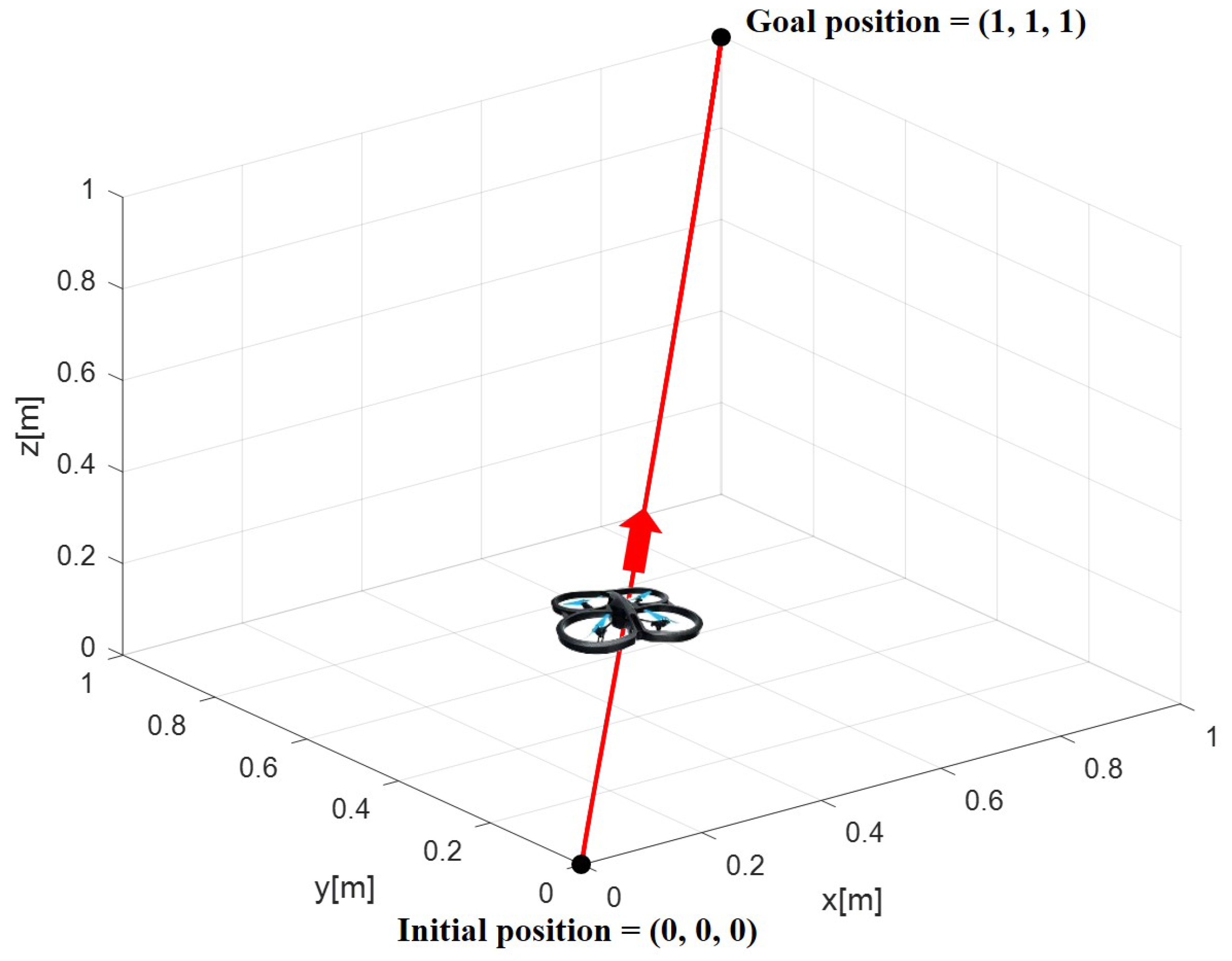
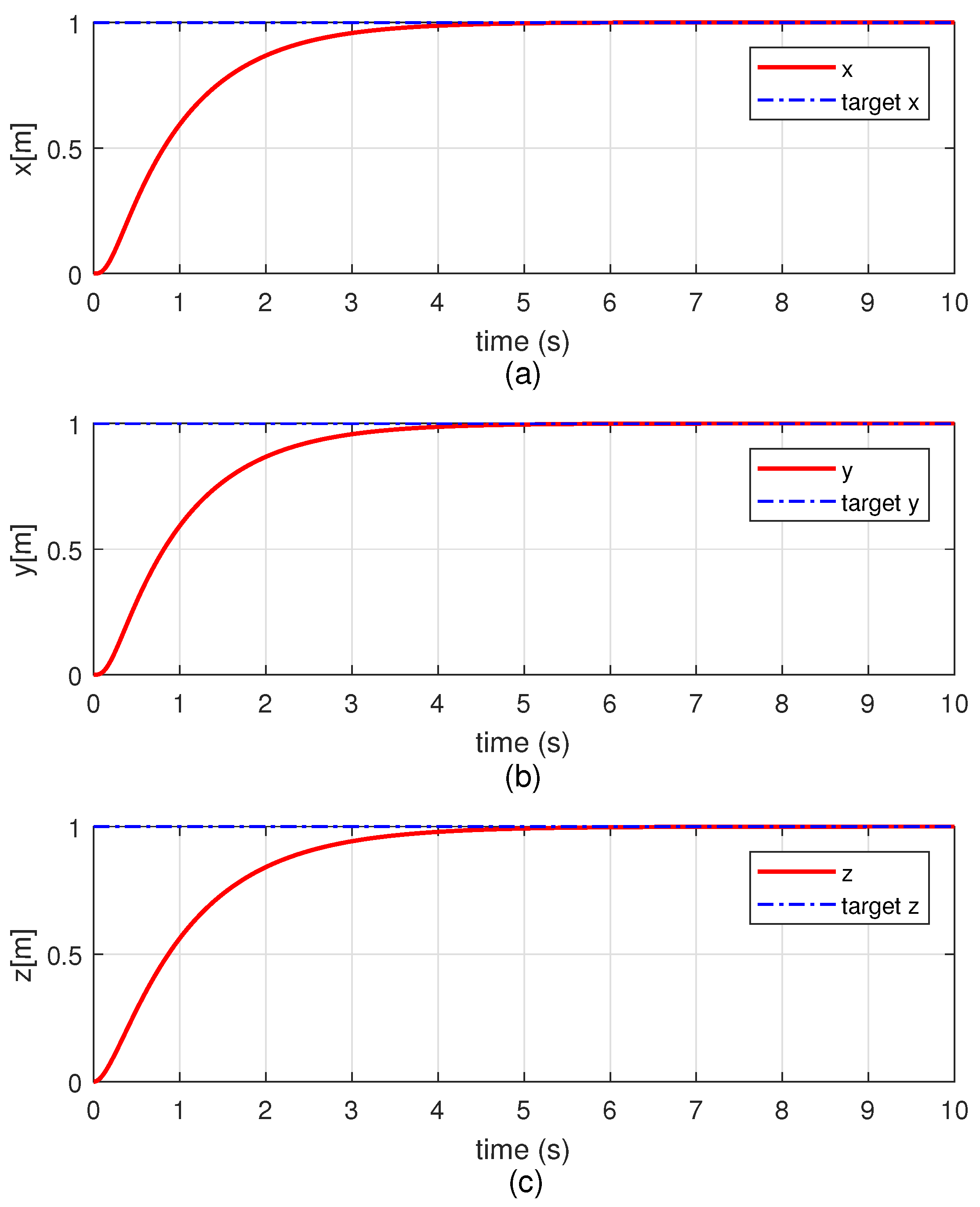
Figure 3 shows the simulation result obtained by applying the inverse optimal position control of a quadrotor, when the initial and target positions are (0, 0, 0), (1, 1, 1), respectively. More details, the time histories of the for each motion of a quadrotor are shown in Figure 4. From the simulation results, we verify that the proposed control method successfully makes a quadrotor move to the target position.
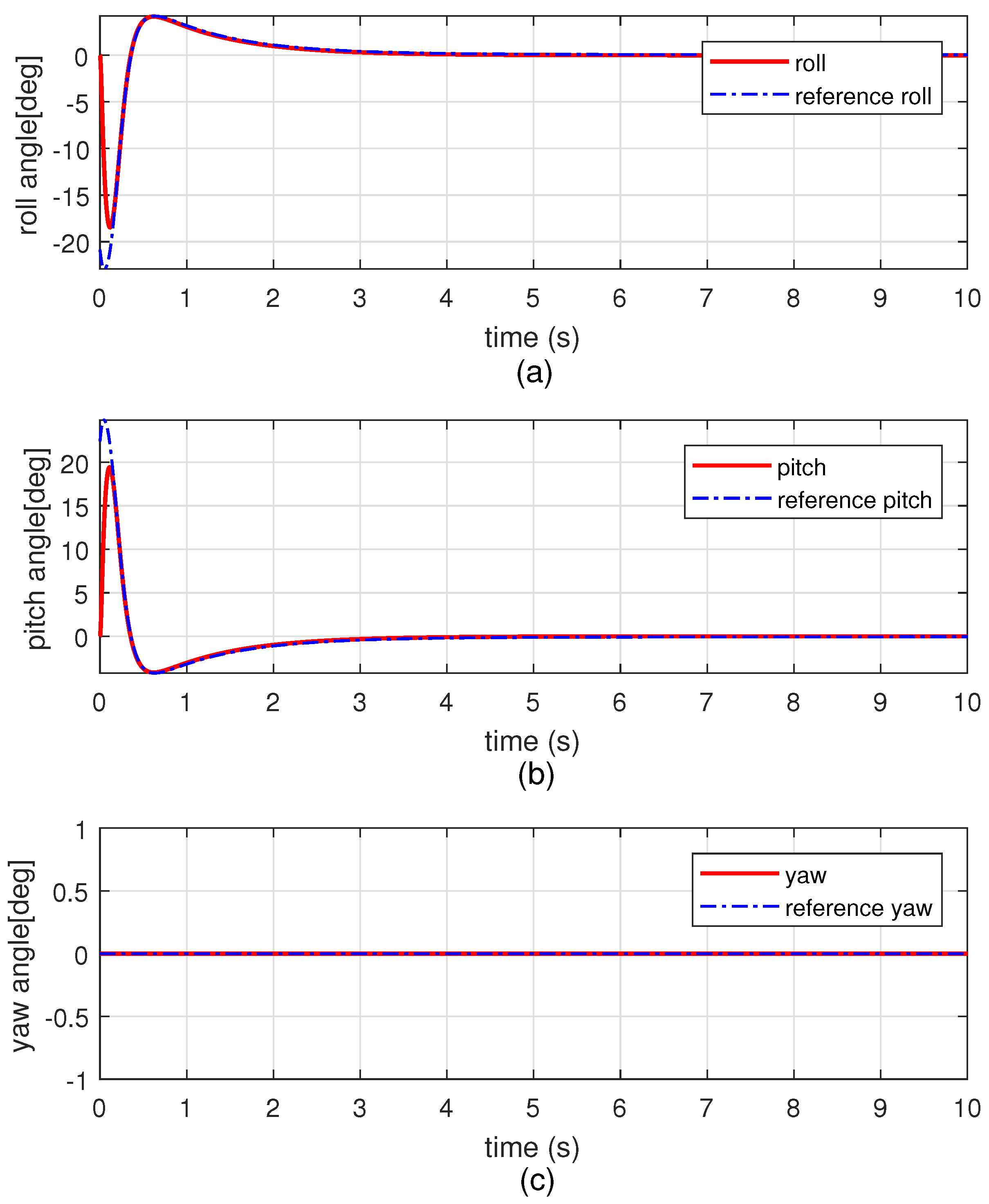
Figure 5 shows simulation results of the attitude control. We can be found that when the initial state of a quadrotor is [rad], the current attitude angles follow the reference attitude angles that enable a quadrotor to converge in the desired position. After a quadrotor reach to the target position, the roll, pitch, and yaw converge to 0, respectively, and then, it maintains a stable posture.
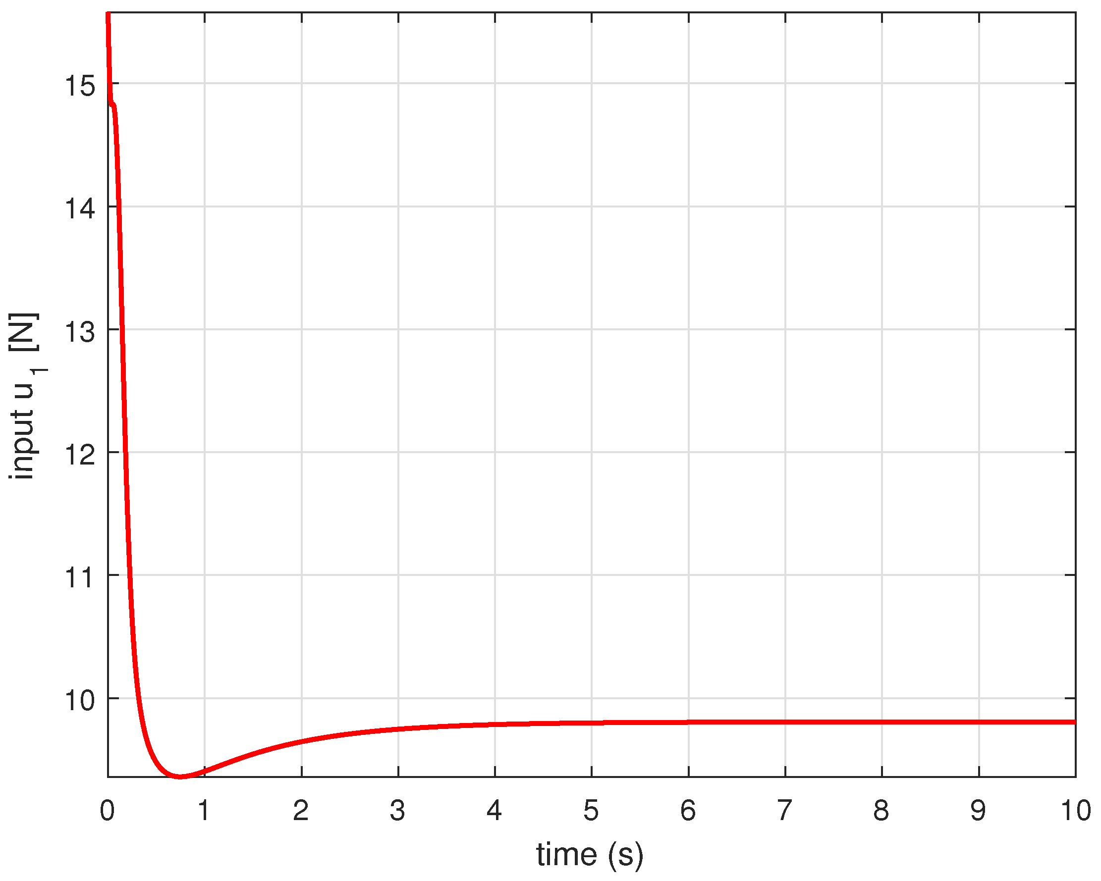
Figure 6 and Figure 7 show the altitude and attitude control inputs of a quadrotor. As shown in the simulation result, the altitude control input is positive value and from 5 s when the quadrotor reaches the target position, is maintained at about 9.8 [N], which is magnitude of gravity. Also we can check that the size changes of input , and are within a reasonable range.
From the simulation results, we verify that the proposed control method successfully makes the position of a quadrotor converge to the references.
We conducted additional simulations to verify that the proposed controller has good performance even though the input coupling matrix changes over time. In the additional simulation, the ascending circular trajectory is set as the reference trajectory, we tested whether the quadrotor track the trajectory well in nonlinear motion.
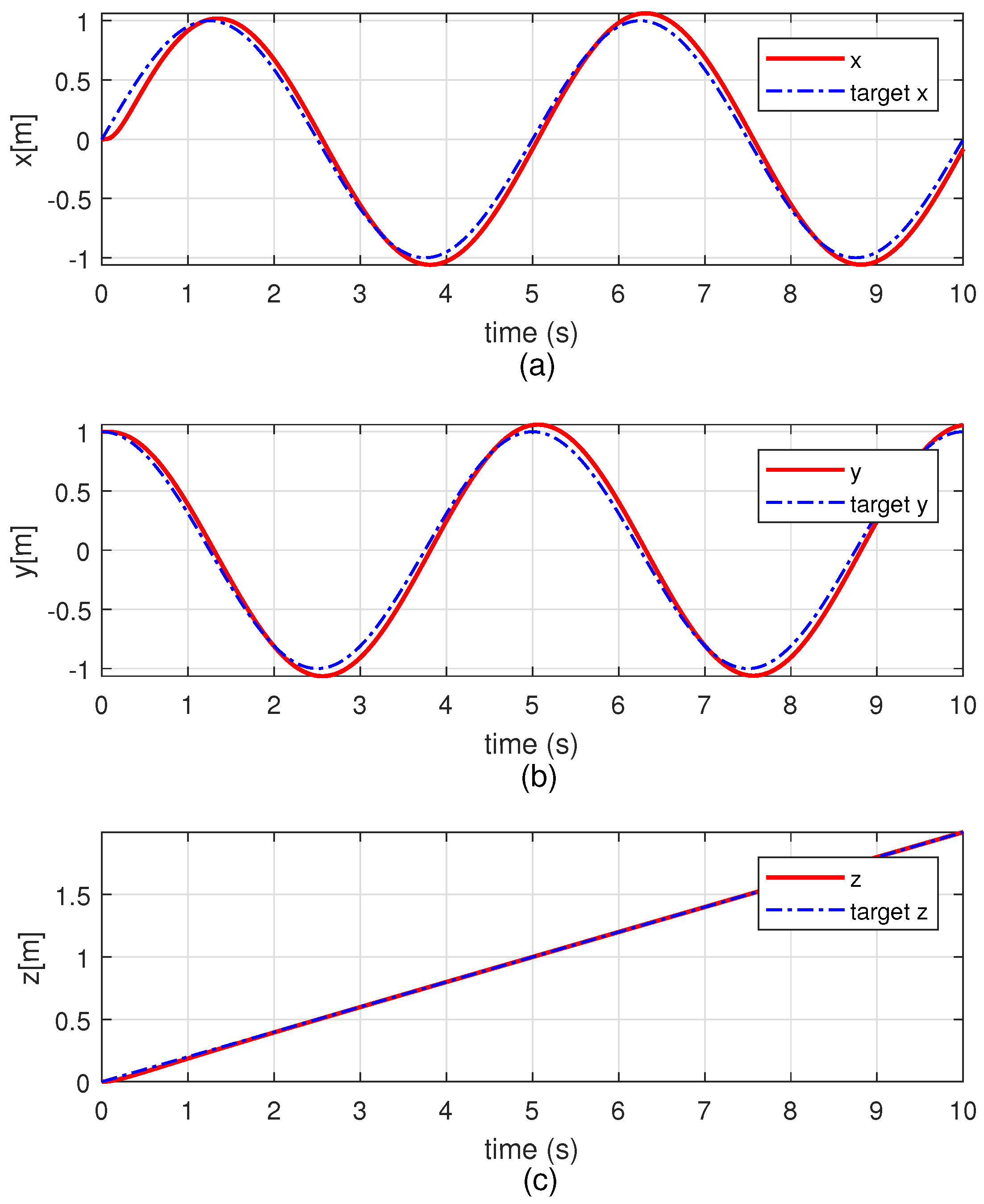
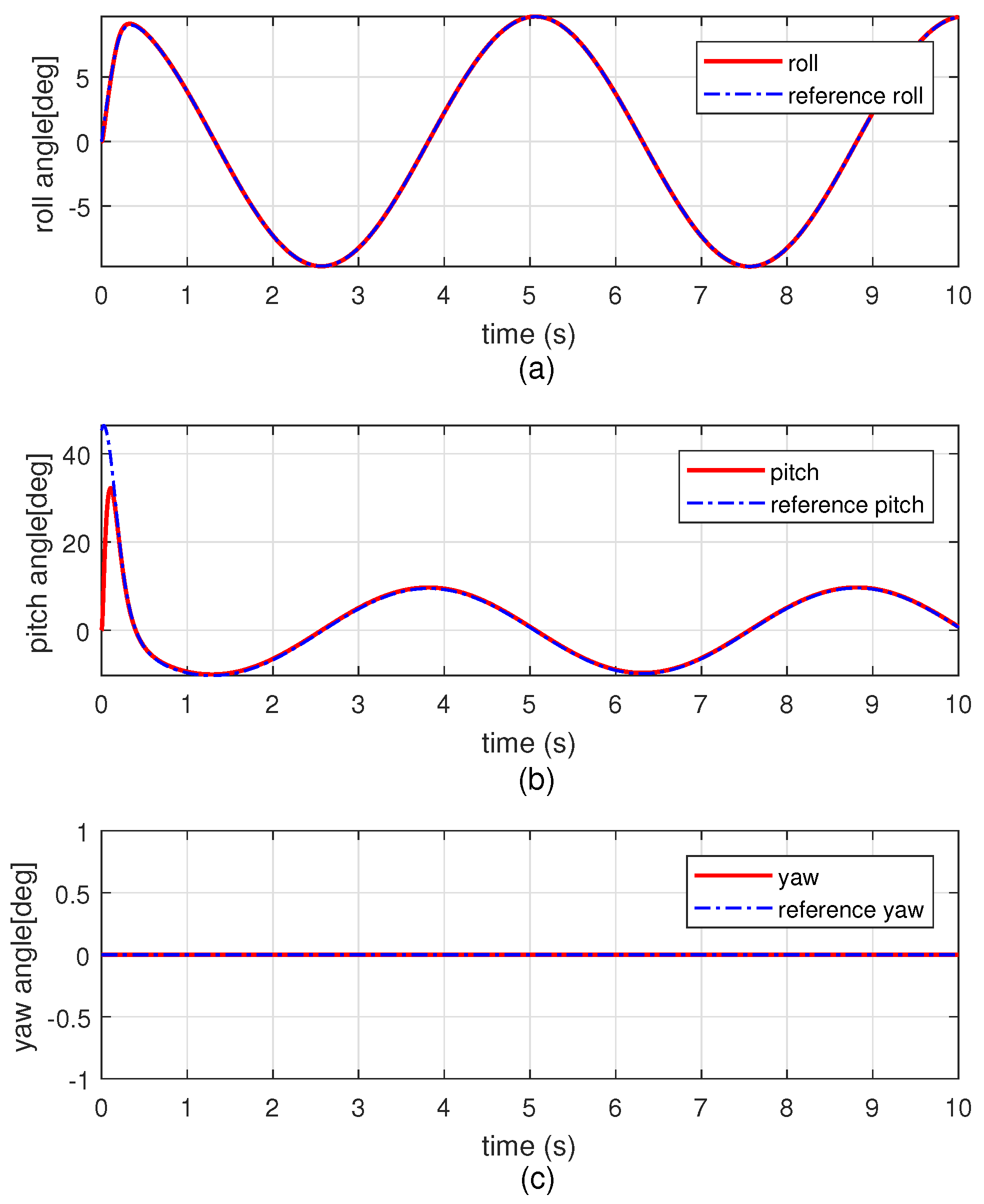
Figure 8 and Figure 9 show that the quadrotor successfully tracking the given trajectory. Figure 10 shows the reference attitude angle for trajectory tracking control. It can be found that the proposed controller maintains good trajectory tracking performance even when the input matrix is changes with time by nonlinear motion such as Figure 10.
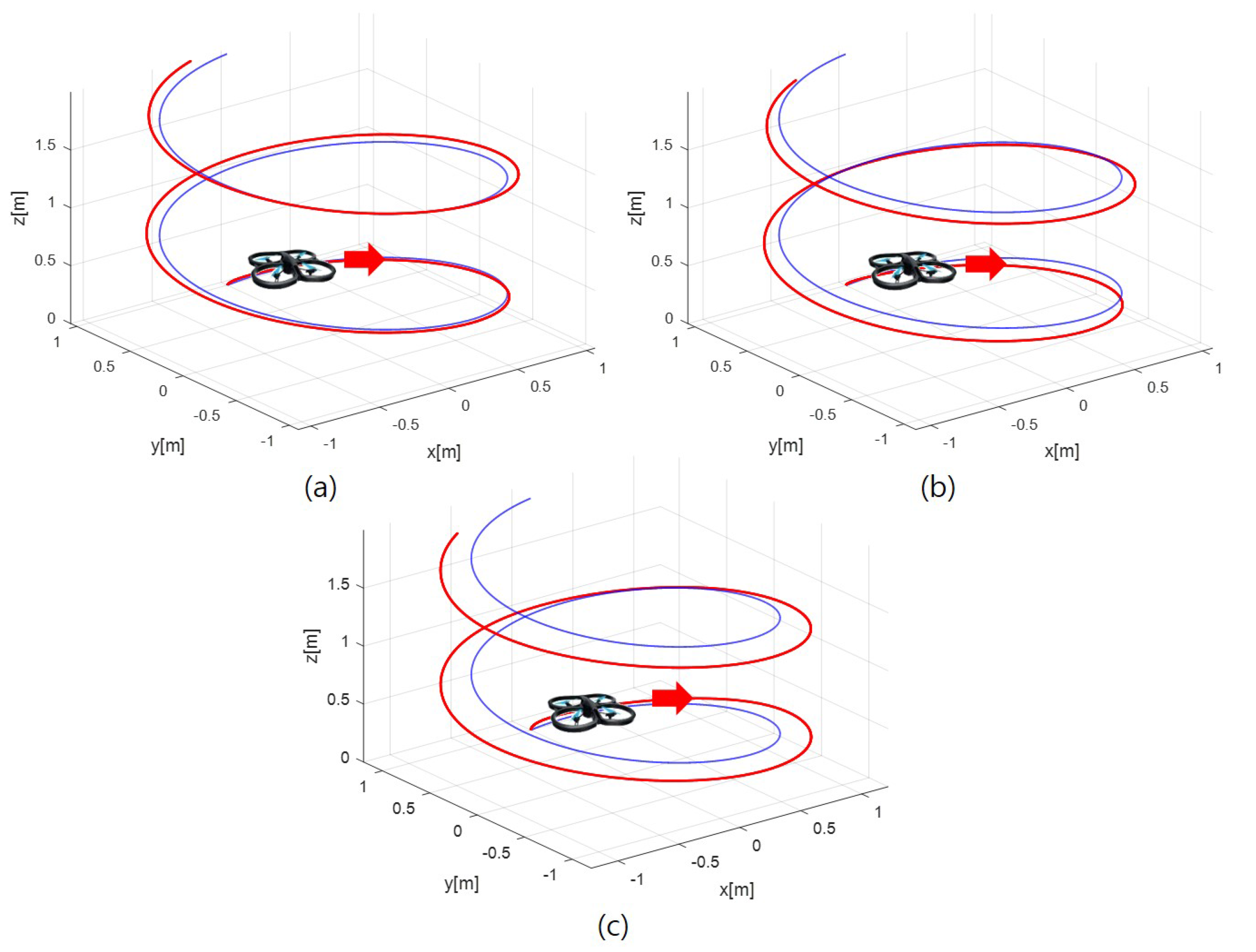
In order to verify the performance of the proposed controller in this paper, we have conducted simulation to compared the performance with other control techniques. In this simulation, the ascending circular trajectory is set as the reference trajectory, we tested whether the quadrotor track the trajectory well in nonlinear motion.
We compared the proposed inverse optimal control, LQR control that is a typical optimal control, and PD control. Since, this paper focuses on position control, so all of the quadrotor attitude control uses the same PID control and same PID gains of attitude. The PID gains of attitude is equal to the gains of the previous simulation. For the PD position control, the control performance depends on the PD gain. Therefore, proper PD gain setting is important for proper performance comparison. To select the proper PD gain, the range of the reference attitude angle and the magnitude of the altitude input were selected in comparison with the other two control methods. Since, the range of the reference attitude angle for position control changes according to the position control gain.
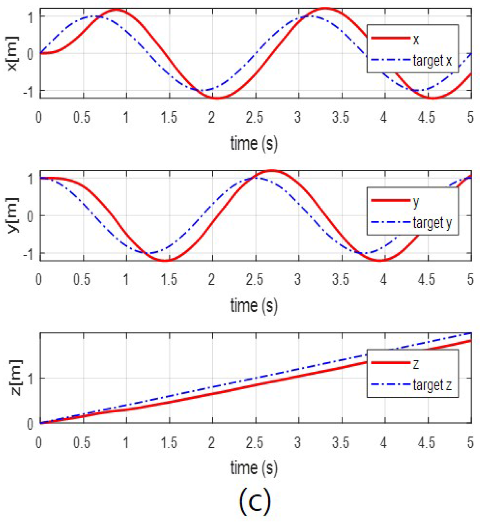
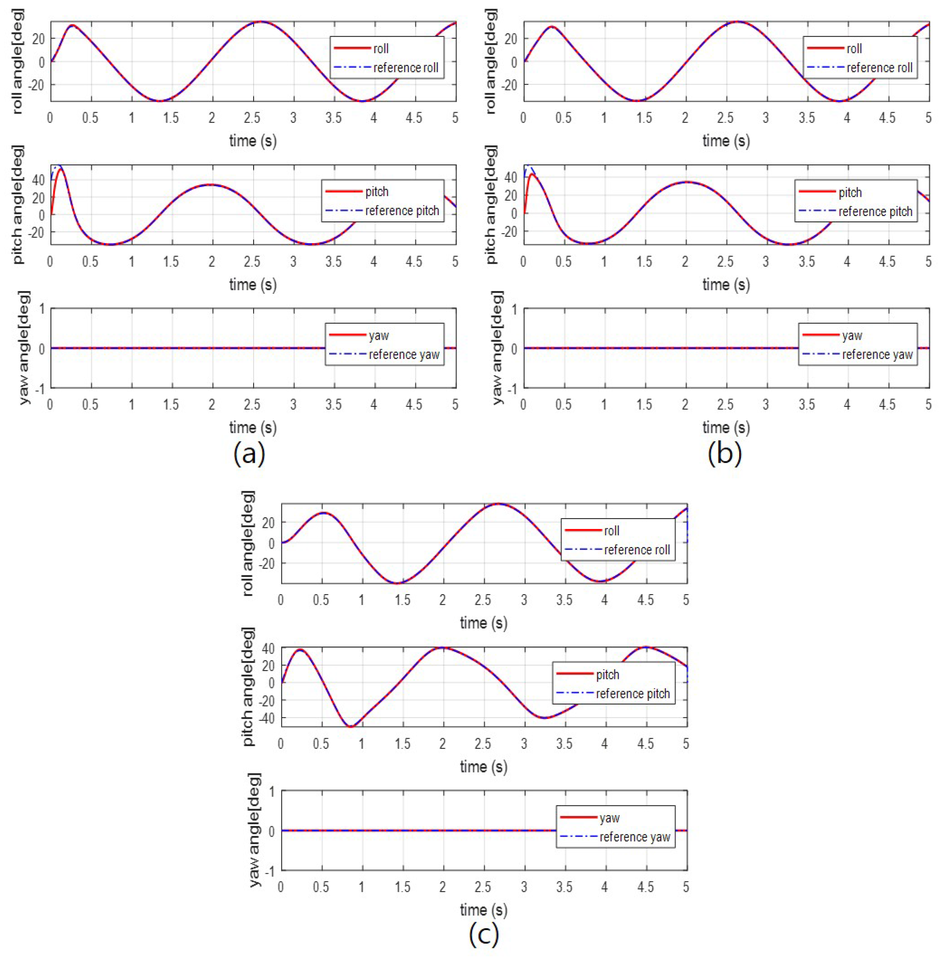
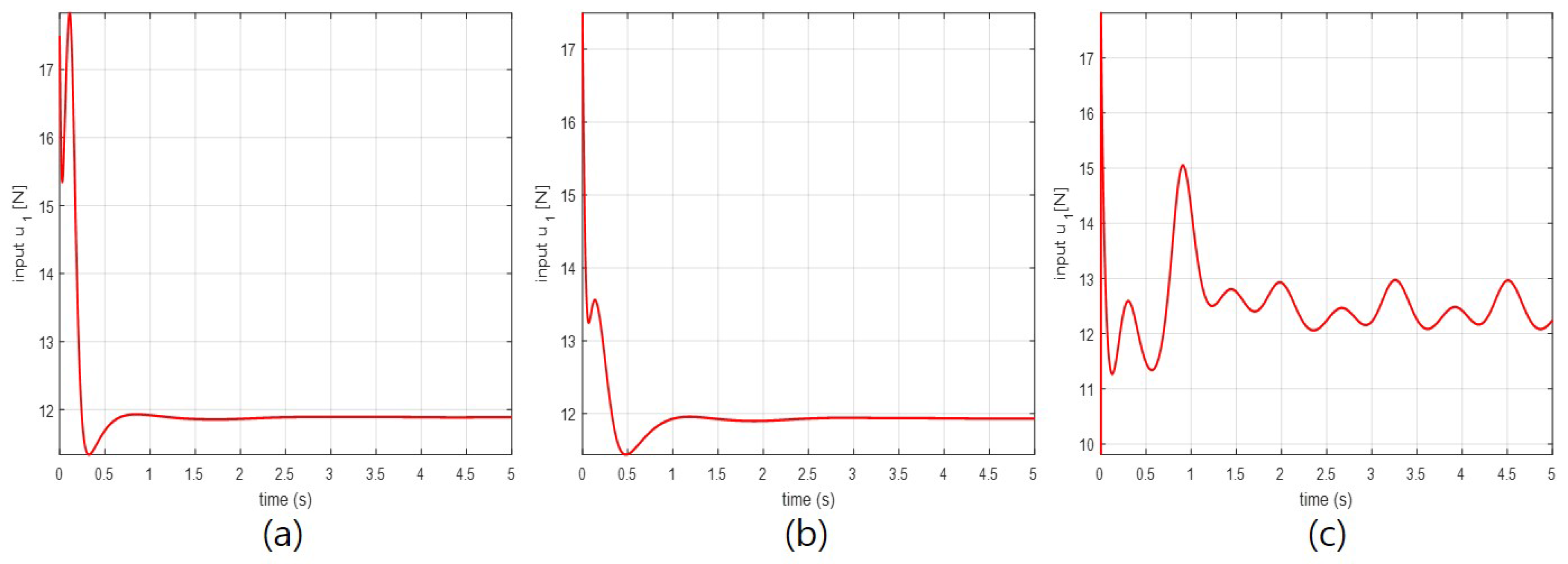
Figure 11 and Figure 12 show trajectory tracking control simulation results for three control methods, when the initial position is (0, 1, 0) with the ascending circular reference trajectory. More details, the time histories of the for each motion of a quadrotor are shown in Figure 12. From the simulation results, we verify that the proposed inverse optimal control has better trajectory tracking performance than other control methods. Figure 13 shows the reference attitude angle for trajectory tracking. In Figure 13, we can see that the attitude of the quadrotor changes continuously around 40 degrees, and if the attitude angle changes greatly, the linear control method like LQR control, PD control does not perform well. The proposed inverse optimal control is an optimal control method for nonlinear system, unlike LQR control method, it can be expected good performance even in the circular trajectory like Figure 11. Looking at the range of attitude angles of Figure 13 and the magnitudes of the inputs of Figure 14 and Figure 15, we can see that the three control methods are simulated in very similar conditions.
Along with the simulation results, we can say the advantage of inverse optimal is in terms of nonlinearity and optimality. The proposed inverse optimal control is of great significance that we dealt with the optimal concept in a nonlinear system and we can find an optimal solution. Simulation results show that the inverse optimal control is better performance because it overcomes the limitation of LQR that are designed based on linear systems. It is an advantage of inverse optimal control from a nonlinear point of view.
In addition, unlike controllers that are not based on optimal control such as PD controllers, it is possible to control the convergence performance and energy consumption of the controller by adjusting (, ) and (, ). It is an advantage of inverse optimal control from a optimality point of view.
5. Conclusions
In this paper, we focused on the inverse optimal position control of a quadrotor. First, we derived the dynamics of a quadrotor using the Newton-Euler formulation. Then, we presented the state transformation technique to derive the position dynamics from the kinematic and dynamic models of a quadrotor. Based on the obtained results, we proposed an inverse optimal position control technique using the altitude control input of a quadrotor. The stability analysis based on the Lyapunov theorem showed that the proposed control method resulted in the exponential stability of a quadrotor system. In addition, we reinterpreted the optimal control problem for a system with a time varying input matrix as an optimal control problem with a constant matrix by appropriately setting the weighting parameters of the performance index. Using this technique, we proved that the proposed control input is the optimal solution of the objective functional and satisfies inverse optimality. Finally, from the simulation results, we verified that the proposed control method is more effective in terms of nonlinearity and optimality than other controllers.
Acknowledgments
This research was supported by the Basic Science Research Program through the National Research Foundation of Korea (NRF) funded by the Ministry of Science, ICT & Future Planning (No. 2015R1A2A2A01007545).
Author Contributions
All authors discussed the contents of the manuscript. Keunuk Lee contributed to the research idea and the framework of this study. Keunuk Lee and Yoonho Choi designed the inverse optimal controller and proved the inverse optimality. Jinbae Park contributed to the modeling of a quadrotor and stability proof. Keunuk Lee performed the simulation and wrote the paper. All authors analyzed the results of this study.
Conflicts of Interest
The authors declare no conflict of interest.
References
- Erginer, B.; Altug, E. Modeling and PD Control of a Quadrotor VTOL Vehicle. In Proceedings of the 2007 IEEE Intelligent Vehicles Symposium, Istanbul, Turkey, 13–15 June 2007; pp. 894–899. [Google Scholar]
- Oner, K.; Cetinsoy, E.; Unel, M.; Aksit, M.; Kandemir, I.; Gulez, K. Dynamic Model and Control of a New Quadrotor UAV with Tilt-wing Mechanism. IJMME 2008, 2, 12–17. [Google Scholar]
- Castillo, P.; Dzul, A.; Lozano, R. Real-time stabilization and tracking of a four-rotor mini rotorcraft. IEEE Trans. Control Syst. Technol. 2004, 12, 510–516. [Google Scholar] [CrossRef]
- Das, A.; Subbarao, K.; Lewis, F. Dynamic inversion with zero-dynamics stabilisation for quadrotor control. IET Control Theory Appl. 2009, 3, 303–314. [Google Scholar] [CrossRef]
- Bouadi, H.; Bouchoucha, M.; Tadjine, M. Sliding Mode Control Based on Backstepping Approach for an UAV Type-quadrotor. Int. J. Appl. Math. Comput. Sci. 2007, 4, 12–17. [Google Scholar]
- Xu, R.; Ozguner, V. Sliding Mode Control of a class of underactuated systems. Automatica 2008, 44, 233–241. [Google Scholar] [CrossRef]
- Efe, M. Robust Low Altitude Behavior Control of a Quadrotor Rotorcraft Through Sliding Modes. In Proceedings of the 2007 Mediterranean Conference on Control and Automation, Athens, Greece, 27–29 June 2007; pp. 1–6. [Google Scholar]
- Madani, T.; Benallegue, A. Backstepping Control for a Quadrotor Helicopter. In Proceedings of the 2006 IEEE/RSJ International Conference on Intelligent Robots and Systems, Beijing, China, 9–15 October 2006; pp. 3255–3260. [Google Scholar]
- Ashfaq, A.; Wang, D. Modelling and Backstepping-based Nonlinear Control Strategy for a 6 DOF Quadrotor Helicopter. Chin. J. Aeronaut. 2008, 21, 261–268. [Google Scholar]
- Das, A.; Lewis, F.; Subbaroa, K. Backstepping approach for controlling a quadrotor using larange form dynamics. J. Intell. Robot. Syst. 2009, 56, 127–151. [Google Scholar] [CrossRef]
- Raffo, G.; Ortega, M.; Rubio, F. An integral predictive/nonlinear control structure for a quadrotor helicopter. Automatica 2010, 46, 29–39. [Google Scholar] [CrossRef]
- Dierks, T.; Jagannathan, S. Output feedback control of a quadrotor UAV using neural networks. IEEE Trans. Neural Netw. 2010, 21, 50–66. [Google Scholar] [CrossRef] [PubMed]
- Alexis, K.; Nikolakopoulos, G.; Tzes, A. Model predictive quadrotor control: Attitude, altitude and position experimental studies. IET Control Theory Appl. 2012, 6, 1812–1827. [Google Scholar] [CrossRef]
- Lai, L.; Yang, C.; Wu, C. Time-Optimal Control of a Hovering Quad-Rotor Helicopter. J. Intell. Robot. Syst. 2006, 45, 115–135. [Google Scholar] [CrossRef]
- Krstic, M.; Tsiotras, P. Inverse Optimal Stabilization of a Rigid Spacecraft. IEEE Trans. Autom. Control 1999, 44, 1042–1049. [Google Scholar] [CrossRef]
- Honglei, A.; Jie, L.; Jian, W.; Jianwen, W.; Hongxu, M. Backstepping-Based Inverse Optimal Atiitude Control of Quadrotor. Int. J. Adv. Robot. Syst. 2013, 10. [Google Scholar] [CrossRef]
- Efe, M. Neural network assisted computationally simple piλdμ control of a quadrotor UAV. IEEE Trans. Ind. Inform. 2011, 7, 354–361. [Google Scholar] [CrossRef]
- Movric, K.; Lewis, F. Cooperative optimal control for multiagent systems on directed graph topologies. IEEE Trans. Autom. Control 2013, 59, 769–774. [Google Scholar] [CrossRef]
- Khalil, H. Nonlinear Systems, 3rd ed.; Prentice Hall: New York, NY, USA, 2002. [Google Scholar]
- Jeong, S.; Seul, J.; Tomizuka, M. Attitude control of a quad-rotor system using an acceleration-based disturbance observer: An empirical approach. In Proceedings of the 2012 IEEE/ASME International Conference on Advanced Intelligent Mechatronics (AIM), Kachsiung, Taiwan, 11–14 July 2012; pp. 916–921. [Google Scholar]
- Bouabdallah, Samir, A.N.; Siegwart, R. PID vs. LQ control techniques applied to an indoor micro quadrotor. In Proceedings of the 2004 IEEE/RSJ International Conference on Intelligent Robots and Systems, Sendai, Japan, 28 September–2 October 2004; pp. 2451–2456. [Google Scholar]
Figure 1.
The coordinates and thrusts of a quadrotor.

Figure 2.
The overall control scheme for the quadrotor position control.

Figure 3.
The inverse optimal position control when the initial and final states are (0, 0, 0) and (1, 1, 1), respectively.
Figure 3.
The inverse optimal position control when the initial and final states are (0, 0, 0) and (1, 1, 1), respectively.

Figure 4.
The position control results for each of the three axes. The dashed line indicates the goal position of each axis, and the solid line is the result of the simulation about each axis: (a) x; (b) y; (c) z.
Figure 4.
The position control results for each of the three axes. The dashed line indicates the goal position of each axis, and the solid line is the result of the simulation about each axis: (a) x; (b) y; (c) z.

Figure 5.
The attitude response for the position control. The dashed line indicates the reference attitude angles that enable the quadrotor to converge in the desired position, and the solid line is the result of the simulation about attitude responses of a quadrotor: (a) ; (b) ; (c) .
Figure 5.
The attitude response for the position control. The dashed line indicates the reference attitude angles that enable the quadrotor to converge in the desired position, and the solid line is the result of the simulation about attitude responses of a quadrotor: (a) ; (b) ; (c) .

Figure 6.
The control input for the altitude of a quadrotor.

Figure 7.
The control inputs for the attitude of a quadrotor: (a) ; (b) ; (c) .
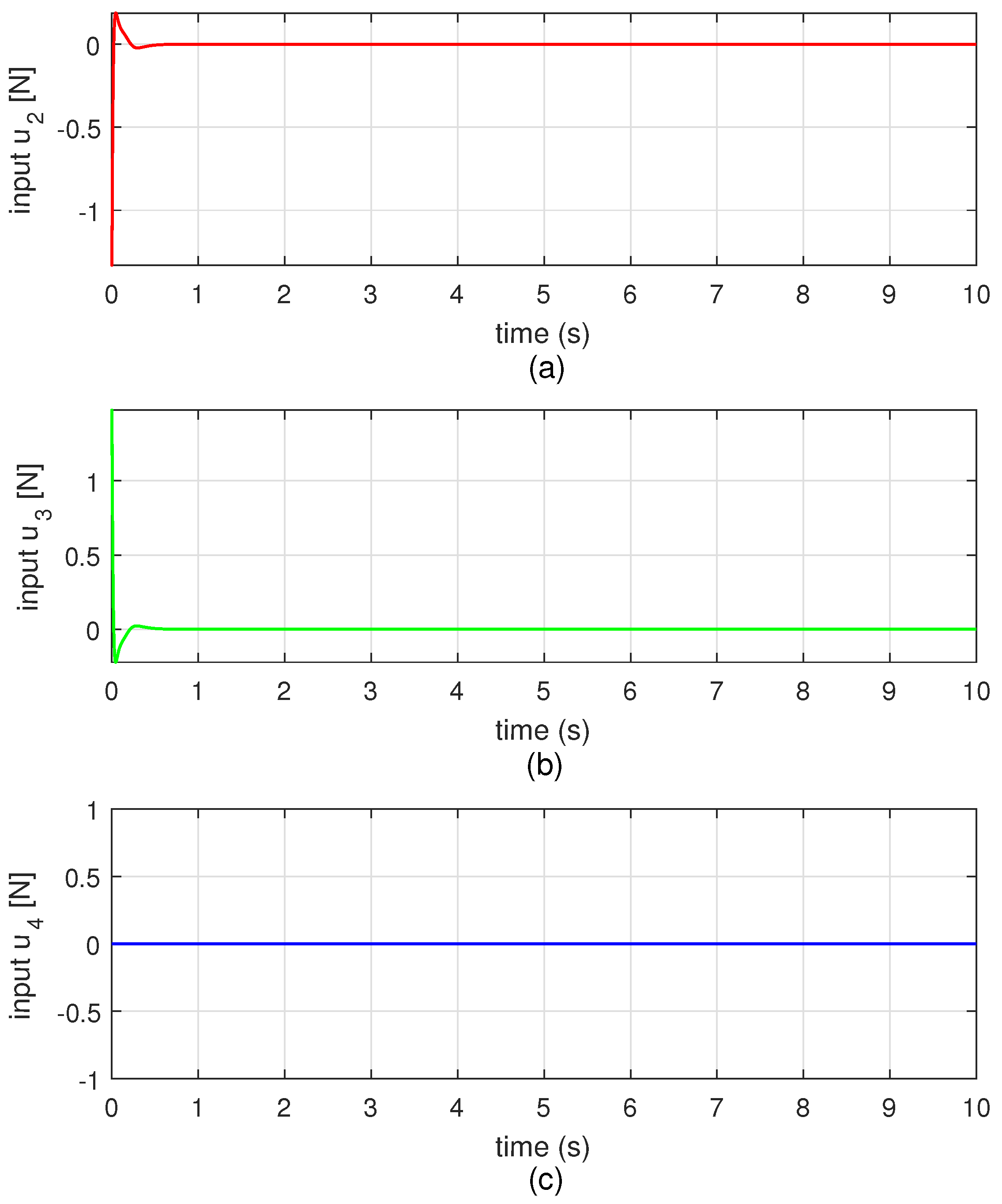
Figure 8.
The trajectory tracking control of a quadrotor. The dashed blue line indicates the reference trajectory and the solid red line is the result of the simulation.
Figure 8.
The trajectory tracking control of a quadrotor. The dashed blue line indicates the reference trajectory and the solid red line is the result of the simulation.
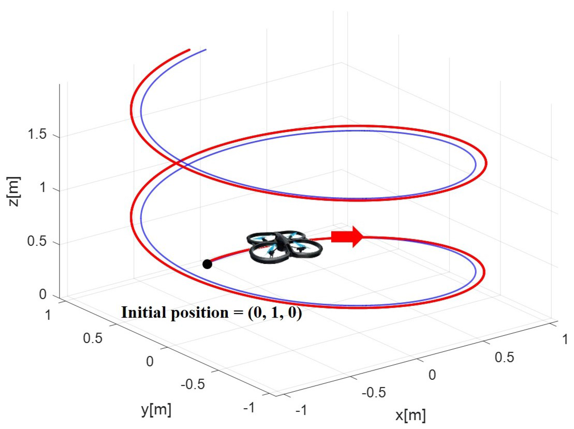
Figure 9.
The trajectory tracking control results for each of the three axes. The dashed line indicates the reference trajectory of each axis, and the solid line is the result of the simulation about each axis: (a) x; (b) y; (c) z.
Figure 9.
The trajectory tracking control results for each of the three axes. The dashed line indicates the reference trajectory of each axis, and the solid line is the result of the simulation about each axis: (a) x; (b) y; (c) z.

Figure 10.
The attitude response for the trajectory tracking control. The dashed line indicates the reference attitude angles that enable the quadrotor to converge in the desired trajectory, and the solid line is the result of the simulation about attitude responses of a quadrotor: (a) ; (b) ; (c) .

Figure 11.
Circular trajectory tracking control results: (a) Inverse optimal control; (b) LQR control; (c) PD control.
Figure 11.
Circular trajectory tracking control results: (a) Inverse optimal control; (b) LQR control; (c) PD control.

Figure 12.
Circular trajectory tracking control results for each of the three axes: (a) Inverse optimal control; (b) LQR control; (c) PD control.
Figure 12.
Circular trajectory tracking control results for each of the three axes: (a) Inverse optimal control; (b) LQR control; (c) PD control.
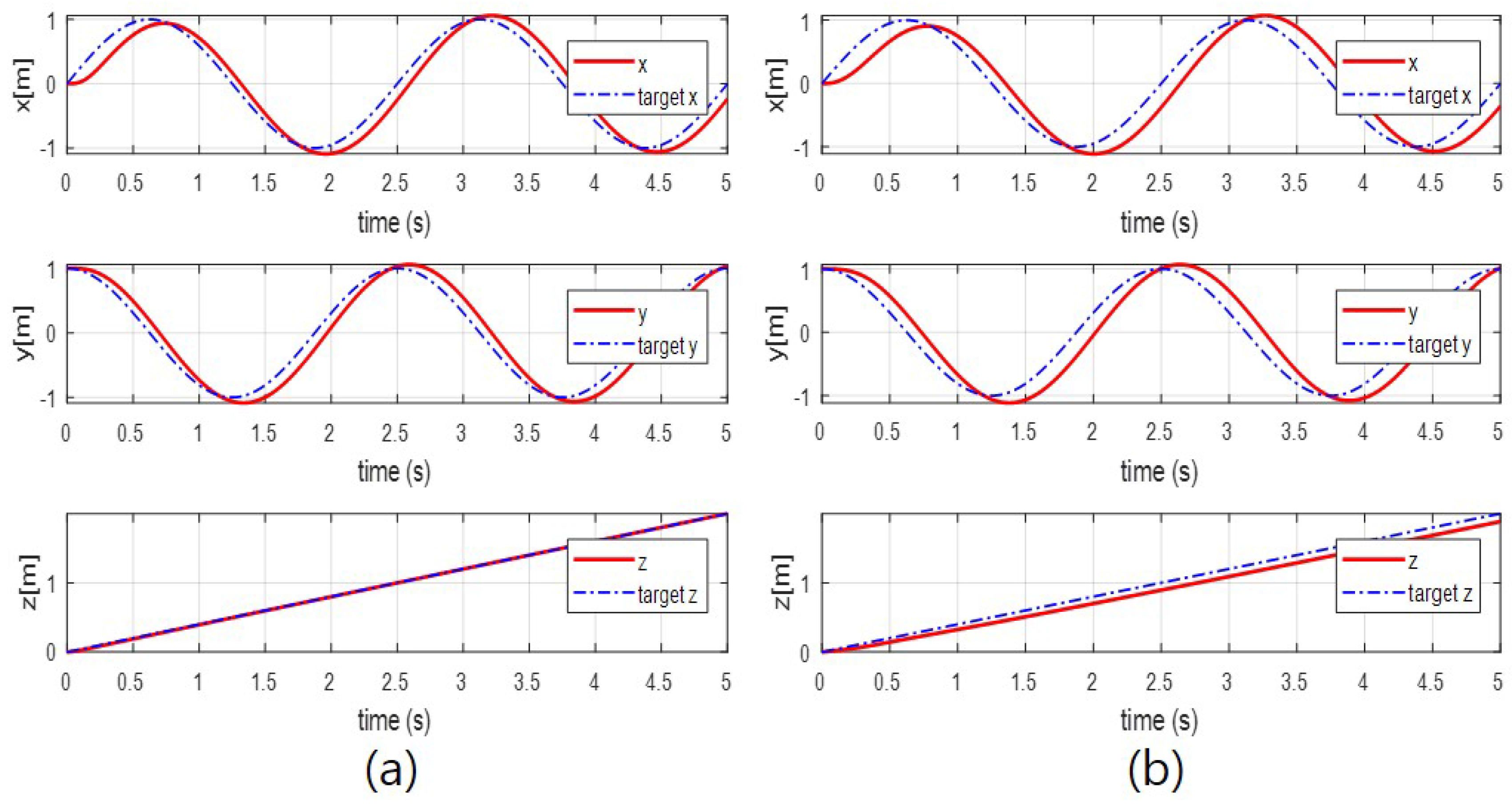

Figure 13.
The attitude response for the trajectory tracking control: (a) Inverse optimal control; (b) LQR control; (c) PD control.
Figure 13.
The attitude response for the trajectory tracking control: (a) Inverse optimal control; (b) LQR control; (c) PD control.

Figure 14.
The control inputs for the attitude of a quadrotor: (a) Inverse optimal control; (b) LQR control; (c) PD control.
Figure 14.
The control inputs for the attitude of a quadrotor: (a) Inverse optimal control; (b) LQR control; (c) PD control.
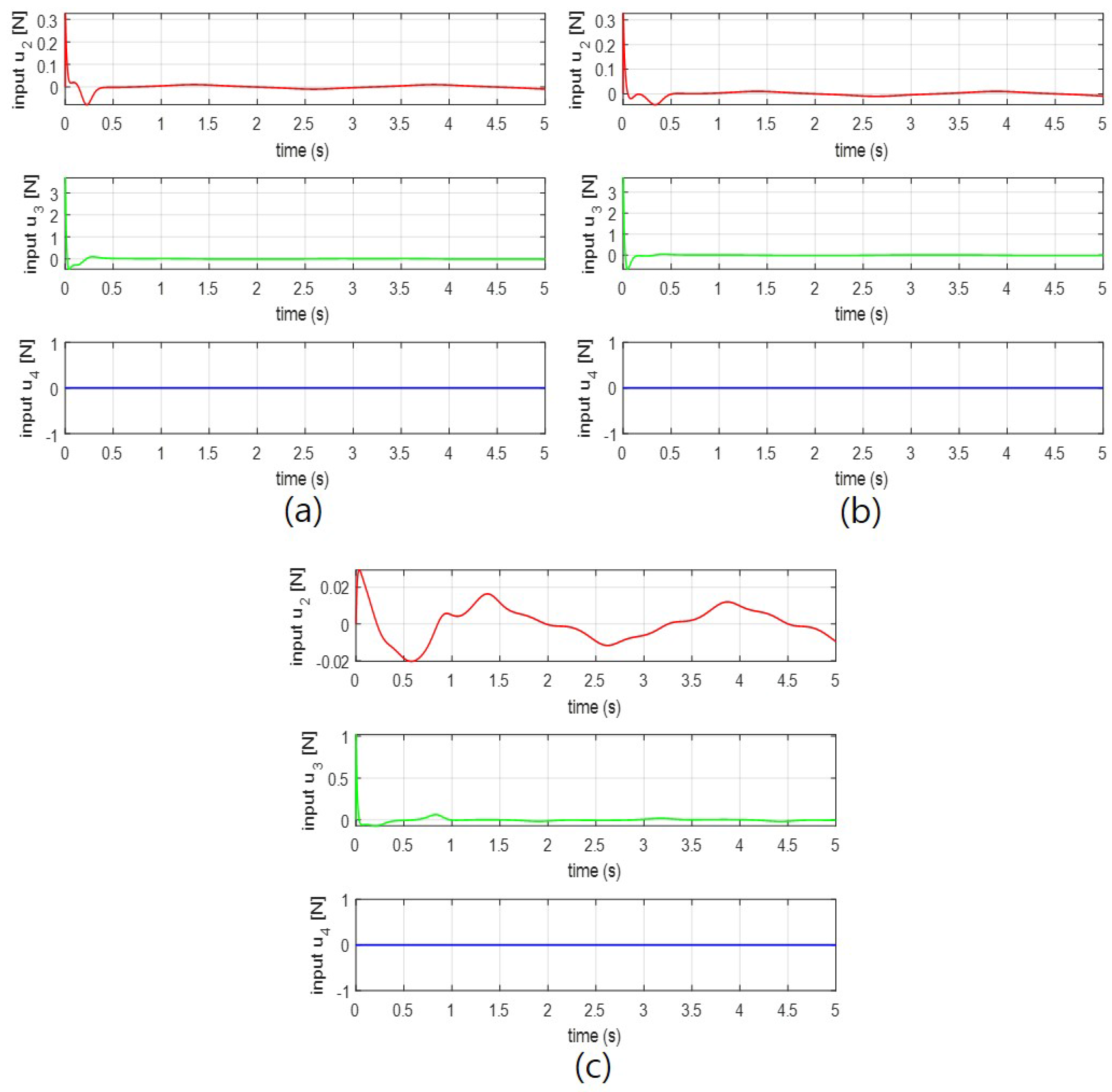
Figure 15.
The control input for the altitude of a quadrotor: (a) Inverse optimal control; (b) LQR control; (c) PD control.
Figure 15.
The control input for the altitude of a quadrotor: (a) Inverse optimal control; (b) LQR control; (c) PD control.


Table 1.
Feedback gains of the position and the rotational controllers.
| Feedback gains of the position controller | |||
| 0.03 | |||
| 0.001 | |||
| PID parameters of rotational controller | |||
| 3 | 3 | 3 | |
| 0.3 | 0.3 | 0.3 | |
| 0.2 | 0.2 | 0.2 | |
© 2017 by the authors. Licensee MDPI, Basel, Switzerland. This article is an open access article distributed under the terms and conditions of the Creative Commons Attribution (CC BY) license (http://creativecommons.org/licenses/by/4.0/).
Share and Cite
MDPI and ACS Style
Lee, K.U.; Choi, Y.H.; Park, J.B. Inverse Optimal Design for Position Control of a Quadrotor. Appl. Sci. 2017, 7, 907. https://doi.org/10.3390/app7090907
AMA Style
Lee KU, Choi YH, Park JB. Inverse Optimal Design for Position Control of a Quadrotor. Applied Sciences. 2017; 7(9):907. https://doi.org/10.3390/app7090907
Chicago/Turabian StyleLee, Keun Uk, Yoon Ho Choi, and Jin Bae Park. 2017. "Inverse Optimal Design for Position Control of a Quadrotor" Applied Sciences 7, no. 9: 907. https://doi.org/10.3390/app7090907
Note that from the first issue of 2016, this journal uses article numbers instead of page numbers. See further details here.