Frequency Modulation and Erosion Performance of a Self-Resonating Jet
by
 and
and
Wenchuan Liu
1,2,3, 
Yong Kang
1,2,3,*,
Mingxing Zhang
4,
Yongxiang Zhou
5,
Xiaochuan Wang
1,2,3 and
Deng Li
1,2,3 1
Key Laboratory of Hydraulic Machinery Transients, Ministry of Education, Wuhan University, Wuhan 430072, China; [email protected] (W.L.); [email protected] (X.W.); [email protected] (D.L.)
2
Hubei Key Laboratory of Waterjet Theory and New Technology, Wuhan University, Wuhan 430072, China
3
School of Power and Mechanical Engineering, Wuhan University, Wuhan 430072, China
4
Shanghai Marine Equipment Research Institute, Shanghai 200030, China; [email protected]
5
Wuhan Hangda Aero Science & Technology Development CO., LTD, Wuhan 430072, China; [email protected]
*
Author to whom correspondence should be addressed.
Appl. Sci. 2017, 7(9), 932; https://doi.org/10.3390/app7090932
Submission received: 7 August 2017
/
Revised: 7 September 2017
/
Accepted: 7 September 2017
/
Published: 10 September 2017
Abstract
:The self-resonating water jet offers the advantages of both a cavitation jet and a pulsed jet, and thus has been widely used for many practical applications. In the present study, the 120° -impinging edge Helmholtz nozzle was investigated for better erosion performance. The oscillating mechanism was analyzed from both numerical and experimental perspectives. The results showed that the cavitation clouds in the chamber dominate the oscillating frequency. The frequency resulting from the non-linear interaction was also observed in the simulation. The dominant frequency increases linearly as pressure decreases without entrained air. The frequency modulation was achieved through various inspiratory methods, and the modulation range was dependent on the pressure drop. The erosion performance was improved with entrained air, and the improvement was effected by the inspiratory method. The oscillating frequency was determined by the forced frequency of entrained air, and the best erosion performance was achieved at the frequency closest to the fundamental frequency. A feasible method to improve the erosion performance was investigated in this preliminary study, which could provide a guide for practical applications.
1. Introduction
Water jet technology has been developed for a variety of commercial cleaning applications as chemical stripping procedures used today are costly, dangerous to personnel, and environmentally unsafe without substantial controls. The increasing demands of modern industry promote the rapid development of water jet technology, and advanced water jet technologies, such as cavitating water jets and pulsed water jets, have been introduced continually. In contrast to non-cavitating jets, cutting is achieved by the energy from collapsing cavitation bubbles. The pressure from these imploding bubbles is extremely high, and is focused at many small areas on the eroding surface [1]. As for the pulsed water jet, it takes advantage of the water hammer pressures produced by the slugs’ impact (which are much higher than the stagnation pressures generated by a continuous jet) and cycling of loading [2]. The use of a fluidic oscillator to achieve the pulsed performance was investigated [3]. Besides, several self-resonating nozzle design concepts, which integrate cavitating jets and pulsed jets, have been developed [4,5,6]. The oscillations are obtained passively without any moving parts and no need for any additional external source of power, which makes these nozzles superior to conventional nozzles. However, there are also some limitations for these self-resonating nozzles since strong oscillations are only achieved in a certain range of both geometrical and operating parameters [7].
Considerable promise has been assigned to the Helmholtz nozzle due to its high efficiency and simplicity. Morel [8] concluded that jet instabilities coupled with the Helmholtz resonance can generate very powerful pressure oscillations with the jet frequency slightly higher than the fundamental frequency of the resonator. Liao and Tang [9] optimized the shape of the impinging edge based on equations of the disturbance wave and two-dimensional vortex, which are the two predominant sources of the generation of pulsation and cavitation. They found that a conical impinging edge with an angle of 120° (Figure 1) outperformed other nozzles with different impinging edges. The three elements (jet shear-layer instability, Helmholtz resonance, and a coupling (feedback) mechanism) of the loop accounted for the oscillating mechanism [10]. Liao and Tang [11] also concluded that the vapor around the bulk flow acts as an accumulator due to its compressibility. This theory, termed the Gas-Spring Theory, inspired scholars to design nozzles in which the jet is modulated by the vapor phase rather than acoustic modulation. This LPHF nozzle (whose working condition is low pressure and high flow rate) has been proven to enhance cleaning efficiency. Although having similar configurations, the LPHF nozzle and conventional Helmholtz nozzles have different optimal ranges of structural and operating parameters due to different oscillating mechanisms. For the conventional Helmholtz nozzle, the high frequencies (order of kHz) involved, corresponding to sound wave lengths in water of less than 0.3 m, suggest that acoustic oscillator or resonator concepts should be of particular interest [7]. As for the LPHF nozzle, the oscillating period is 3–5 s [12], which means the time of phase transition is more than the relaxation time of the jet passing through the cavity, and the vapor phase is predominant in the oscillating process.
To have a better understanding of the vapor phase effect on the oscillating mechanism, numerous experiments have been conducted to study cavitation structures. The various limitations of the measurement techniques have resulted in notable efforts to use numerical simulations for cavitating flows in recent years. Based on the assumption of a homogenous equilibrium medium proposed by Kubota et al. [13], many cavitation models have been proposed which require the mixture density to be defined. One approach to this kind of model was based on the state equation [14,15]. Another model was a multiphase cavitation mixture model based on the transport equation for the phase change. An additional equation for the vapor (or liquid) volume fraction, including source terms for evaporation and condensation (i.e., bubble growth and collapse), was introduced by Merkle et al. [16]. Similar techniques with different source terms were adopted by Kunz et al. [17], Habil [18] and Singhal et al. [19]. There have been various comparative studies of the various cavitation models [20,21,22,23]. In 2014, the four-equation cavitation model was proposed by Goncalvès [24], which is very attractive for studying thermodynamic effects and cryogenic cavitation.
As the vapor phase plays an important role in the oscillating process in the LPHF nozzle, due to its compressibility, air could be also introduced for frequency modulation. Besides, the air–water jet is capable of enhancing the material removal efficiency and can be controlled for specific machining operations. Momber [25] concluded that the material removal rate became sensitive to the amount of air supplied and became a maximum value corresponding to an optimum air flow-rate. The air–water jet technology was also applied in oil drilling, proposed by Kolle [26], to help increase the rate of penetration (ROP). Hu [27] conducted experiments on specimens impinged by the pulsed air–water jet. It turned out that the air entrained into the cavity significantly affects the material removal rate. For the LPHF nozzle, there are fierce entraining and momentum transports around the bulk flow due to sudden expansion. As a result, a negative pressure zone occurs in the oscillating chamber. The air intake can be achieved simply by drilling suction holes around the circumference of the chamber. In addition, Liao and Tang [11] conducted preliminary experiments in which the suction hole was intermittently blocked by fingers, and significant changes in the oscillating pressure were observed. They also claimed that oscillations will be enhanced if the suction hole is closed when the air cluster contracts, but kept open when the air cluster expands.
It transpired that the air–water jet from a LPHF nozzle could not only improve the material removal rates but could also be used for frequency modulation. While limited research has focused on the frequency modulation of the LPHF nozzle via intake air, especially with the forced air excitation, it is reasonable to speculate that the frequency characteristics and the erosion efficiency of the LPHF nozzle is interrupted by the air intake. In this paper, both the experimental method and the simulation are introduced in Section 2. In the discussion, the Gas-Spring Theory is verified from both the numerical simulation and experimental perspectives. The paper then looks at how the effects of air intake on the oscillating frequency was investigated, as well as the range of frequency modulation. Finally, it looks at how the erosion experiments were conducted to evaluate the efficiency of the air–water jet with forced air excitation at various frequencies.
2. Research Method
2.1. Experimental Method
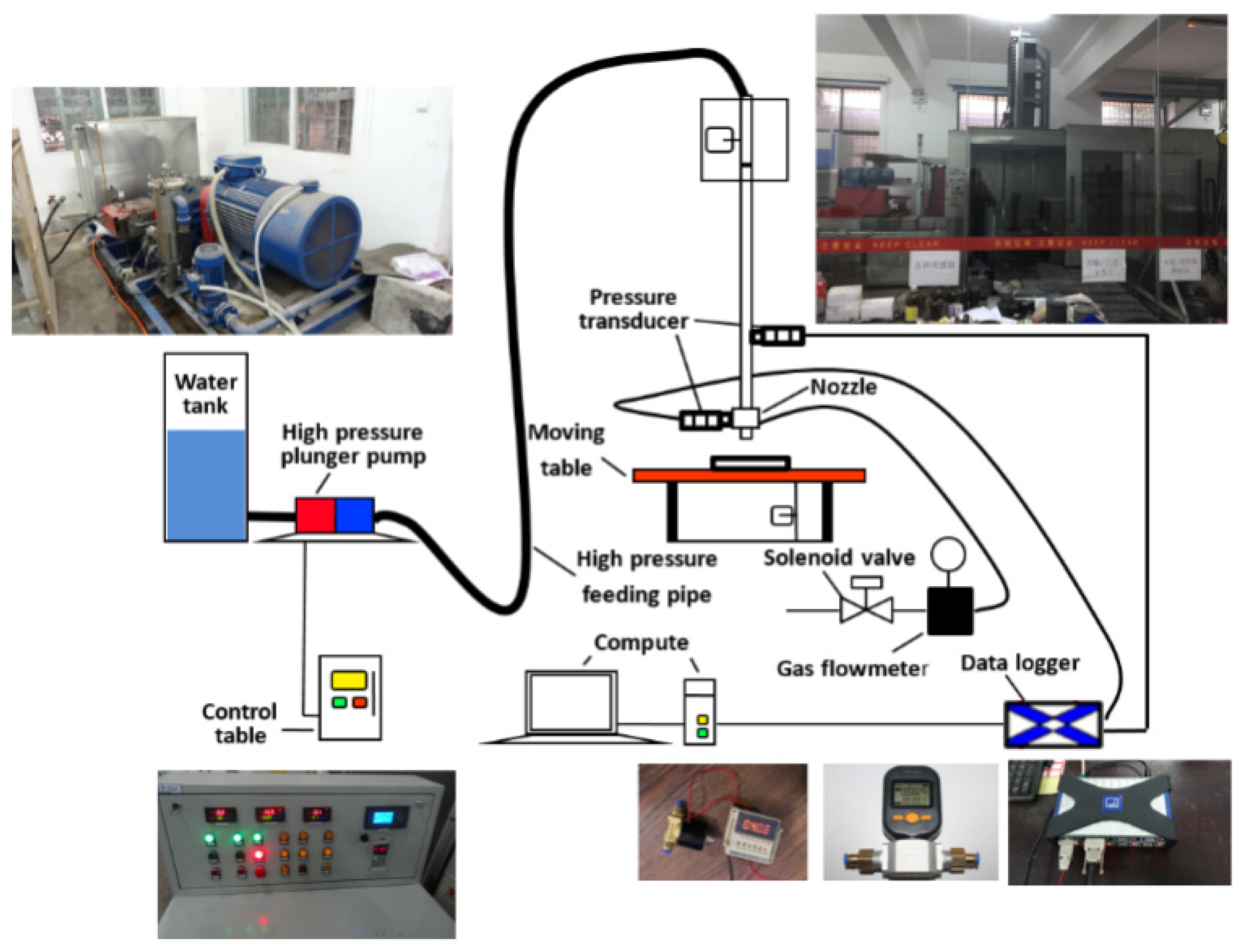
The experiment was conducted with the use of a multifunctional water jet test bench (Figure 2) developed by our research team independently. The flow was supplied from a high-pressure plunger pump with a maximum flow rate of 120 L/min. A pressure transducer (Model: CY100) was installed immediately next to the nozzle inlet, and the inlet pressure of each test could be accurately controlled. The other pressure transducer was positioned on the nozzle to measure the pressure fluctuations in the oscillation chamber. All pressure transducers used in experiments had been calibrated by the manufacturers, and the main uncertainty in this experiment was the accuracy of the pressure transducer, which was less than ±0.5% FS (full scale). Each process of pressure acquisition was 60 s and the sampling frequency was set to 100 Hz. Bessel lowpass was used to eliminate the electronic signals caused by the motor with a frequency of 50 Hz. The Hilbert–Huang transform (HHT) combined with empirical mode decomposition (EMD) [28] were adopted in filtering and analyzing the pressure signals, as the oscillations were characterized by being non-linear and non-stationary.
The specimens were clamped into a holder, and then mounted on the moving table. The moving table had both X and Y motions with an accuracy of 0.1 mm. In each erosion test, the moving table was moved away from the jet impact region before the pressure was maintained at the setting value. The moving table was then moved to adjust the specimen to be collinear with the axis of the nozzle. During each test, the specimen was exposed to the jet for 90 s. The standoff distance for the nozzle could be varied by sliding the input pipe vertically and clamping it into place at the desired setting. However, a fixed standoff distance of 60 mm was used for all tests.
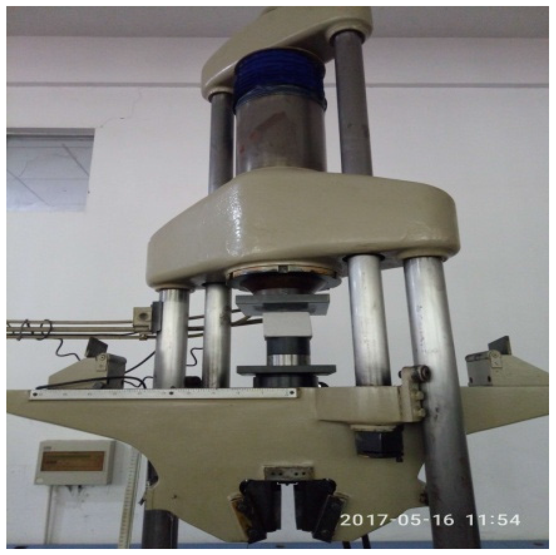
The specimen adopted in the present study had the dimensions of mm. The compressive strength was measured by a material testing machine (Figure 3). The mean value of the compressive strength was 2.561 MPa within the tolerance scope from −4.76% to 7.53%.
The volume removed was measured by filling the generated cavities with fine-grained salt with a density of . These salts were then removed and weighed with the use of an electronic balance (Figure 4) with resolution to 0.1 mg. The volume removed was then calculated through Equation 1.
where is the salt mass used to fill the erosion cavity.
The erosion area, which gad an irregular shape with a slightly serrated border (Figure 5), could be achieved by the method of line tracing in Photo Shop. To be more specific, the erosion area was encircled by creating a spline in Photo Shop and the pixels of erosion were obtained. The real areas were calculated as follows:
where is the number of pixels per square centimeter in reality.
To reduce the impact of casual factors, all results were averaged for further analysis.
The Helmholtz nozzle used in the experiment is shown in Figure 6, and was designed according to the optimal structure with the JMP method by Wang [29]. The upstream nozzle had an inlet diameter of = 13 mm, a convergent angle of , and an outlet diameter of = 5.9 mm. The chamber diameter was constant with = 72 mm and the chamber length, = 36.6 mm. A downstream nozzle was used with = 10.7 mm. There were four suction holes of = 2 mm with a uniform distribution around the circumference of the chamber according to the simulation results by Zhou [30]. A fitting was used for connecting the jet bench and the nozzle. Air pipes, originating from the suction holes, were connected with the gas flow meter and the solenoid valve (controlled by the relay), and finally connected to the atmosphere. The amount of air, measured by the gas flow meter, was controlled by the number and position of the suction holes. The passage for air suction was impeded periodically with use of the solenoid valve and relay.
The testing itself was conducted according to a schedule given in Table 1. The set of data obtained for a given choice of both number and the distribution of open suction holes was called a “series”. Every series then consisted of 3–4 “runs”, each covering various pressure drops and forced exciting frequencies. The description of the opening holes is presented in Figure 7 (from a top view).
2.2. Numerical Simulation Setup
The numerical simulation was also performed to verify the Gas-Spring Theory. The axisymmetric two-dimensional computation domain and boundary conditions are shown in Figure 8. The inflow velocity was adjusted appropriately until the time averaged inlet pressure agreed with the experimental inlet condition ( = 1.5 MPa). The constant outlet pressure was set to 1 atm, as the absolute pressure was adopted in the current simulation. It is assumed that inlet and outlet areas were in a pure liquid region and the volume fraction of water in these boundaries were set as 1 in the present study.
Other boundaries were the same as the non-slip walls. Geometrical parameters were the same with the experimental nozzle. The time step was set as s to capture the periodical variation of the two-phase flow instead of the real transient evolution of the cavitating flow. According to the Gas-Spring Theory, the collective bubbles act as accumulators and were investigated in the present study. Although the collective bubbles consist of small bubbles, the variation of small bubbles and their interaction were not the aim of this study. Data acquisition took place at each time step. To obtain the multiple oscillating periods, the whole simulation time was 25 s.
The standard computational grid was composed of orthogonal cells. A special form of stretching the mesh was applied in the main flow direction just after the chamber inlet, so the two-phase flow area was efficiently simulated. In the other direction, stretching was also applied close to the walls and the shear layer. Grid independence tests were performed, and the grid size was increased by 50% each time until no noticeable variance in the velocity profile was observed. In this study the investigation of the mesh’s influence was performed by monitoring the axial velocity (normalized by the maximal velocity) within 10 s. The average streamwise velocity around the shear layer was also investigated, because the shear layer plays an important role in the oscillating mechanism. The monitoring lines are presented in Figure 9.
The results of grid convergence are presented in Figure 10. There was no obvious difference in the average axial velocity for the three mesh cases, while mesh 1 deviated from the other mesh cases in the velocity distribution around the shear layer, especially for the position near the impinging edge (lines 4–6). Due to no noticeable variance between mesh 2 and mesh 3 in the velocity profiles, mesh 2 was selected as final mesh for the present simulation. Mesh 2 contained 14,281 nodes with the minimum length of 0.066 mm streamwise and of 0.1 mm in the vertical direction. The model equations were solved by the finite-volume method. The time-dependent governing equations were discretized in both space and time domains with the SIMPLE algorithm. The first-order upwind scheme was used for spatial discretization. The unsteady first-order implicit formulation was implemented for the transient term. It was found that within 20 iterations in each time step, the RMS (root-mean-square) residuals satisfied the current convergence criteria, which was specified as at least a three orders of magnitude decline in the volume fraction of the vapor phase and a six-order decline in the mass conservation equation.
In the present paper, the cavitating flow was modeled using the single fluid approach by treating the two liquid/vapor phases as a homogenous mixture. The equations of mass and momentum of the mixture for the single fluid approach are given as:
where and are the velocities in the coordinate direction and respectively, p is the pressure, and is the mixture density. and are the dynamic viscosity and the turbulent viscosity.
An additional transport-based equation is introduced for the vapor phase volume fraction to model the cavitation process:
where represents the mass transfer source term, which is determined by the cavitation model. The density and viscosity of the mixture fluid are calculated as follows:
where subscripts l and v stand for the liquid and vapor phase, respectively.
The source term in Equation (5) can be further rearranged in the general form:
The source terms and represent the effects of evaporation and condensation during the phase change and are derived from the bubble dynamics equation for the generalized Rayleigh–Plesset equation as follows:
The bubble radius is related to the vapor volume fraction and the bubble number density , as:
To reduce the turbulence dissipative terms in the cavitation regions, a modified RNG turbulence model was implemented into the ANSYS Fluent code through the user-defined function (UDF).
In the standard RNG k- model, the turbulent eddy viscosity is defined as:
where , k is the turbulent kinetic energy, and is the turbulent eddy dissipation. The standard RNG k- turbulence model tends to overestimate the turbulent eddy viscosity in the cavity region since it was first proposed for an incompressible single-phase flow. A modified model, which considers the compressibility of cavitating flow, was proposed by Reboud et al. [31] as follows:
where n is the exponential coefficient. This treatment can artificially reduce the turbulent eddy viscosity in the cavitation region based on the vapor volume fraction by adjusting the value of the exponential coefficient. In the current simulation, the value of n was fixed at 10, because this value has been validated for many cases [32,33,34,35].
3. Results and Discussion
3.1. Gas-Spring Theory
The time-resolved chamber pressure signals with various pressure drops are presented in Figure 11, as well as the marginal spectrum obtained from the HHT. Negative pressure oscillations were easily captured by the pressure transducer positioned in the chamber. The absolute values of negative pressure peaks increased with the increasing pressure decline, caused by the intensified turbulent momentum transportation and entrainment between the main jet and the quiescent fluid. Meanwhile, the negative pressure peaks became more intense with higher pressure decline. According to the Gas-Spring Theory, the frequency increase may come from the accumulated time for the cavity cluster in the chamber decreasing as more energy was obtained with a higher pressure decline. To be more specific, the instantaneous energy density (IE) Equation 15 was introduced to check the energy fluctuation (Figure 12). Energy fluctuations were observed in each condition, and the higher the inlet pressure was, the more energy was accumulated for collective bubbles within the same time range. It turned out that the inlet pressure decline affects both the frequency and amplitude of the instantaneous energy density.
where is the energy–frequency–time distribution, which is obtained from the HHT, and is the circular frequency.
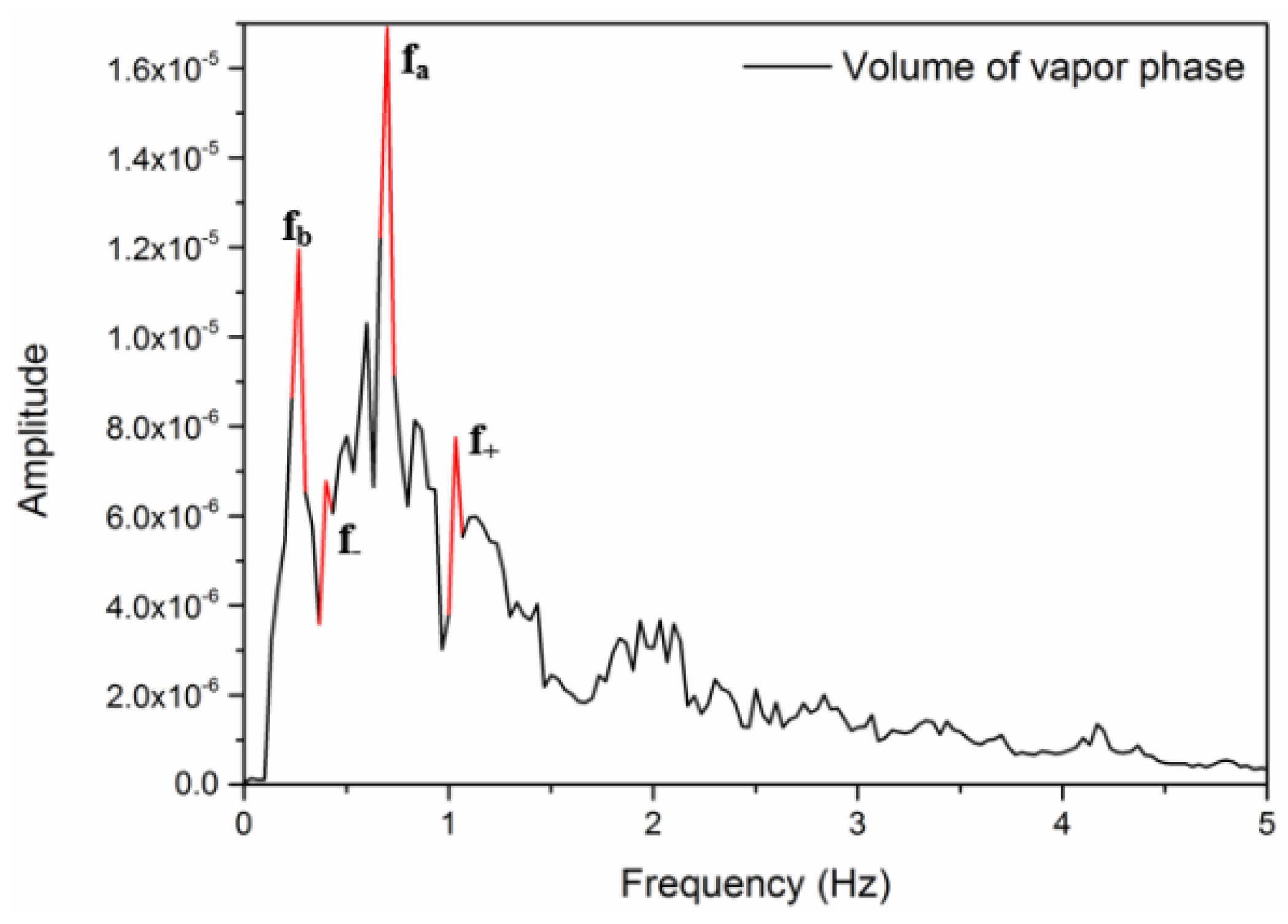
The numerical simulation was also used to verify the Gas-Spring Theory. The marginal spectrum of the volume fraction of the vapor phase is presented in Figure 13, with a sharp peak at 0.700 Hz being observed. Multiple additional right and left peaks can also be observed, along with the dominant , as mentioned in several previous investigations on the cavity flow. They have been denoted = 0.103 Hz and = 0.400 Hz when symmetrically distributed around . In addition, a peak at low frequency, = 0.267 Hz, which is close to the experimental results, was observed. The existence of such a low frequency is a common feature in most of the various configurations [36]. The frequency could result from the non-linear interaction between and , but could also result from the non-linear combination of and , via an amplitude modulation at impingement [37,38,39,40]. Indeed, combinations between the harmonics of fa with occur, to produce sum frequencies . For instance, the = 0.400 Hz is close to the difference frequency = 0.433 Hz. The global structure of the spectral distribution can be viewed as the result of non-linear interactions and modulation processes which may combine, as shown in Miksad et al. [41] and [37,38].
According to the theory of vortex-acoustics, the oscillating frequency could be calculated as follows [42]:
where are denoted as the cross section area and the length of the upstream nozzle; is denoted as the volume of the oscillating chamber; are denoted as the pressure, the adiabatic exponent of air and the volume fraction of vapor phase, respectively.
In the current paper, the structural parameters were calculated according to the experimental conditions to obtain the oscillating frequency:
The vapor phase volume fraction was calculated based on the arithmetic mean value of the vapor phase volume , which was monitored in the simulation case. In the current simulation, the value of is . In order to make the calculations of the theory model possible, the parameters is set equal to 1.4 in the present calculation considering that the mixture flow was dominated by the ambient temperature and pressure conditions [27].
Compared with the calculated oscillating frequency, the low-frequency component of the volume fraction of the vapor phase was much closer to the experimental results. As mentioned by Johnson [7], cavitation apparently does interfere with the modulation mechanism to some degree. It turned out that the cavitation clouds dominated oscillation in the LPHF nozzle. Meanwhile, as the fundamental frequency obtained from experiments (0.263 Hz) was close to the low-frequency component (0.267 Hz) rather than the fundamental frequency (0.700 Hz) in the simulation, the non-linear interactions and modulation process should be of particular interest, which should be considered in future studies.
A typical variation cycle was extracted to better illustrate the time evolution of the predicted turbulent cavitating flow. The time evolution of cavity growth and collapse is shown in Figure 14. The cloud consists of a large number of small bubbles and is more elongated in the streamwise direction. At the start of the typical cycle (), the cavitation clouds emerge in the region near the chamber wall, and a part of the cavity is about to shed itself from the large cavity due to its instabilities at . The overall volume of the primary cavity tends to decrease as the vapor content is intermittently convected out of the cavity by the small clouds (Figure 14c). There are also some cavities in the shear layer around the bulk flow. Then the parallel bubbles form in the chamber, and the upper bubble cluster decreases while the other cluster gradually grows near the bulk flow. These two bubble clusters finally coalesce into the large volume cavity around the bulk flow (Figure 14e) and then shift further downstream and collapse due to the impinging edge. After a series of generation, deformation and motion of the cavities, the small volume cavities will finally coalesce into a larger cavity near the chamber wall, which marks the beginning of the next period.
3.2. Frequency Modulation
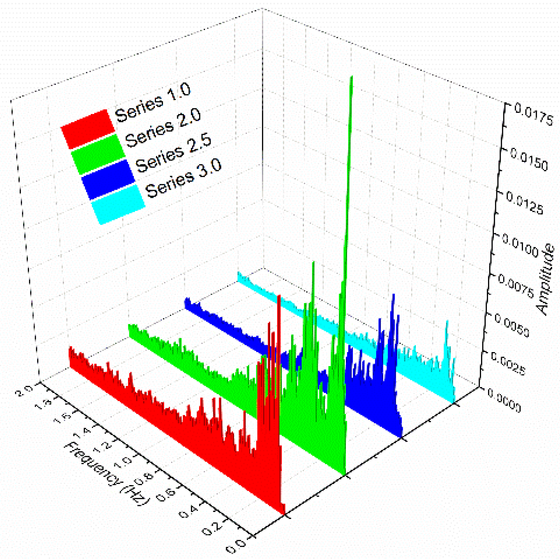
The pressure signals and marginal spectrum with various inspiratory methods are presented in Figure 15 and Figure 16, respectively. By connecting with the atmosphere through the suction hole, the negative pressures of the self-inspiratory jet decreased to some degree, while the absolute peak values of negative pressure decreased drastically with an increasing numbers of suction holes. Meanwhile, a wider frequency range occurred due to the intake air, which means the fluid-field in the chamber became more complicated. Compared with the Figure 11, it transpired that the distribution of suction holes also affected the peak value and the oscillating frequency of the chamber pressure.
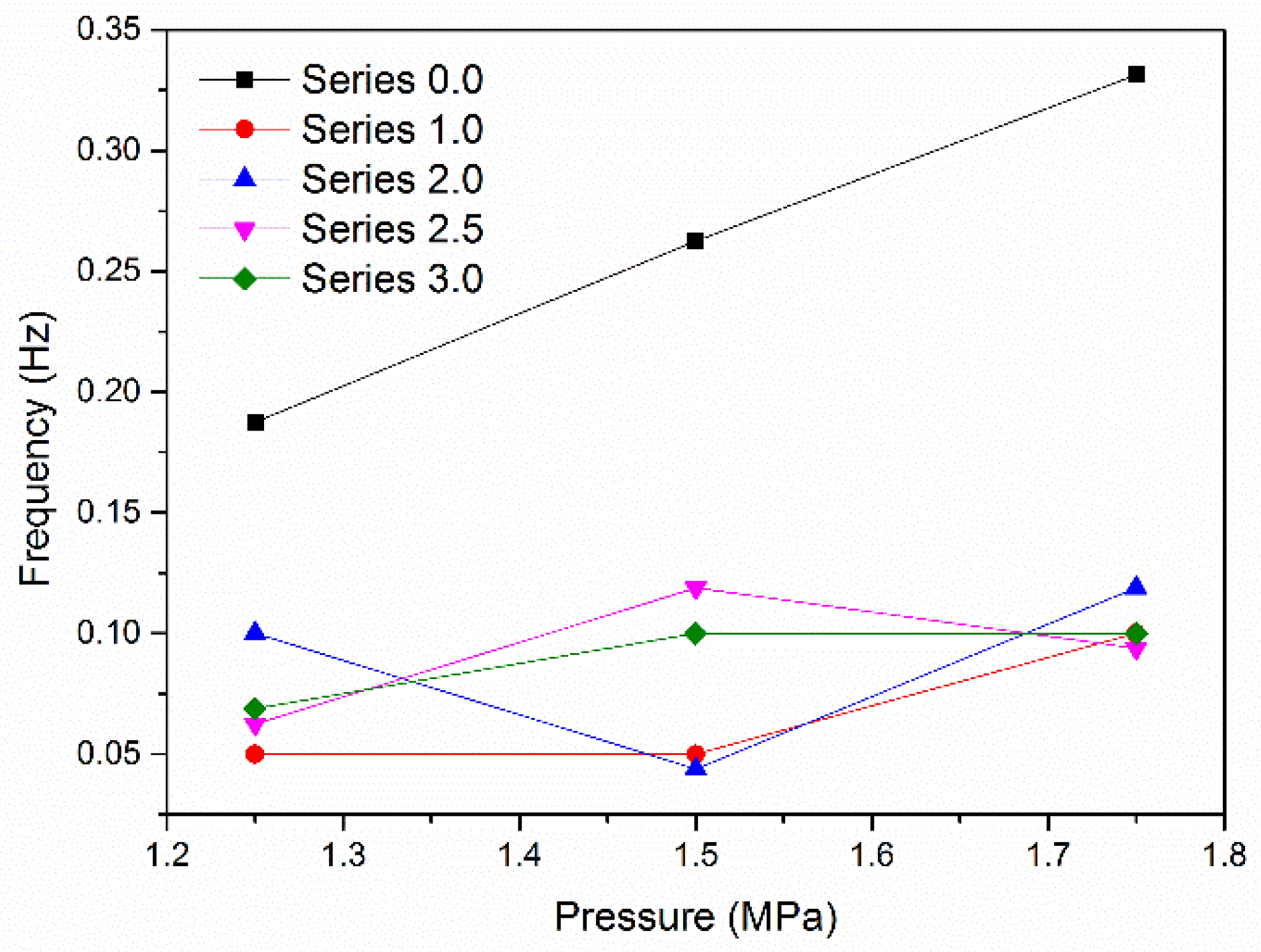
The dominant frequency under various pressure declines via the air intake of the marginal spectrum is presented in Figure 17. Under the different pressure declines, the modulation range was different. While the dominant frequency increased linearly with the pressure decrease, it was observed that the frequency of each inspiratory method did not vary monotonically with the falling pressure. It transpired that the mechanism of frequency modulation was different with/without air intake. Besides, the range frequency modulation was different at various pressure declines. To be more specific, the modulation range was quite large for the case at 1.25 MPa and 1.50 MPa, while quite narrow at the pressure decrease of 1.75 MPa. The oscillating mechanism was rather complicated when air was entrained into the chamber, especially for the multi-hole condition. With a certain nozzle geometry, the oscillating frequency can be attributed to the characteristics of the mixture flow, such as density and bulk modulus of elasticity. Although the average density of the mixture flow was considered to be almost constant, the bulk modulus of elasticity of air is far less than that of water, which causes the bulk modulus of elasticity of the mixture flow to have an appreciable change. Therefore, the compressibility of the mixture flow increased. Besides, the instabilities of the bulk flow were also intensified with the entrained air. The complicated coupling between the bulk flow and air should be considered in further studies based on a large number of experiments and using advanced technology. This preliminary study can provide a guide for practical applications. The frequency modulation was achieved and its effects on the material removal is discussed in the next section.
3.3. Erosion Performance
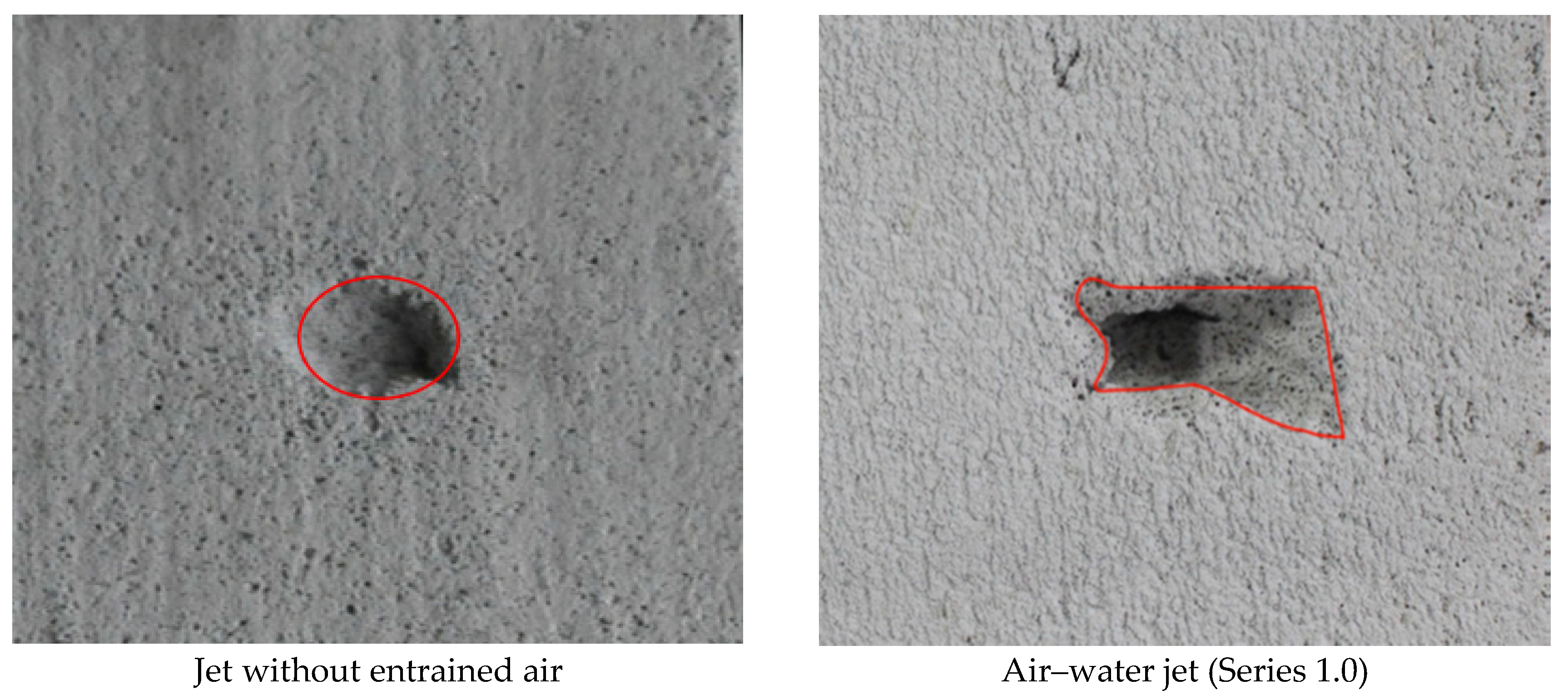
The erosion patterns of concrete specimens are presented in Figure 18. The erosion region caused without air intake was in the shape of a cone, but the erosion region under the action of the air–water jet had an irregular shape due to the air within the jet forcing redial motion.
Using the jet without entrained air for reference, the relative erosion performance of four inspiratory series is compared in Figure 19. The red bars show the influence of the air entrainment on the normalized erosion volume and the blue bars show the normalized erosion area. The erosion performance was improved with the air entrainment to some degree. Assuming that a high number of open suction holes corresponds to a high air-flow rate, it transpired that both air-flow rates and air entry-path affected the erosion performance. Although the cavitation in the chamber was suppressed by the air intake, a moving air coat was created to reduce the friction between the water jet surface and the surrounding air. As the water hammer pressure is attributed to both velocity and the mixture density, there seems to have been a “trade-off” between the jet velocity increase and the mixture density decrease when air was entrained into the chamber. Besides, according to the research by Wright [43], cavitation bubbles move away from the nozzle without expanding much while the gas expands rapidly upon exit after discharging, so the erosion areas with entrained air increase as a result.
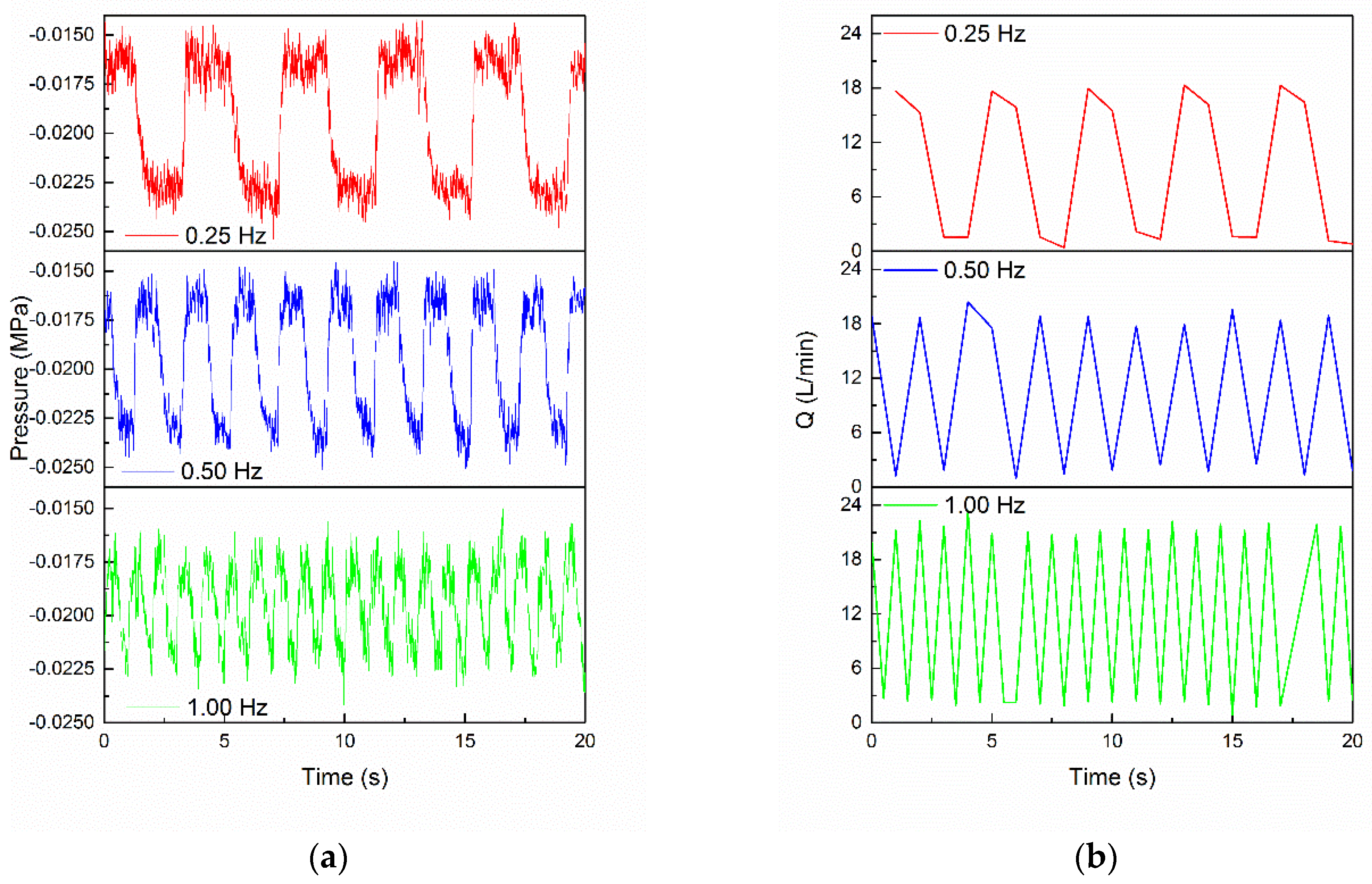
As for the forced air excitation, it transpired that the oscillating frequency of the chamber pressure was completely determined by the forced frequency of air excitation (Figure 20). In the practical applications, the frequency could be modulated at the desired value according to the specified situation by the method of forced air excitation. With increasing forced frequency, the mean volume of entrained air increased due to the fierce entraining and momentum transportation.
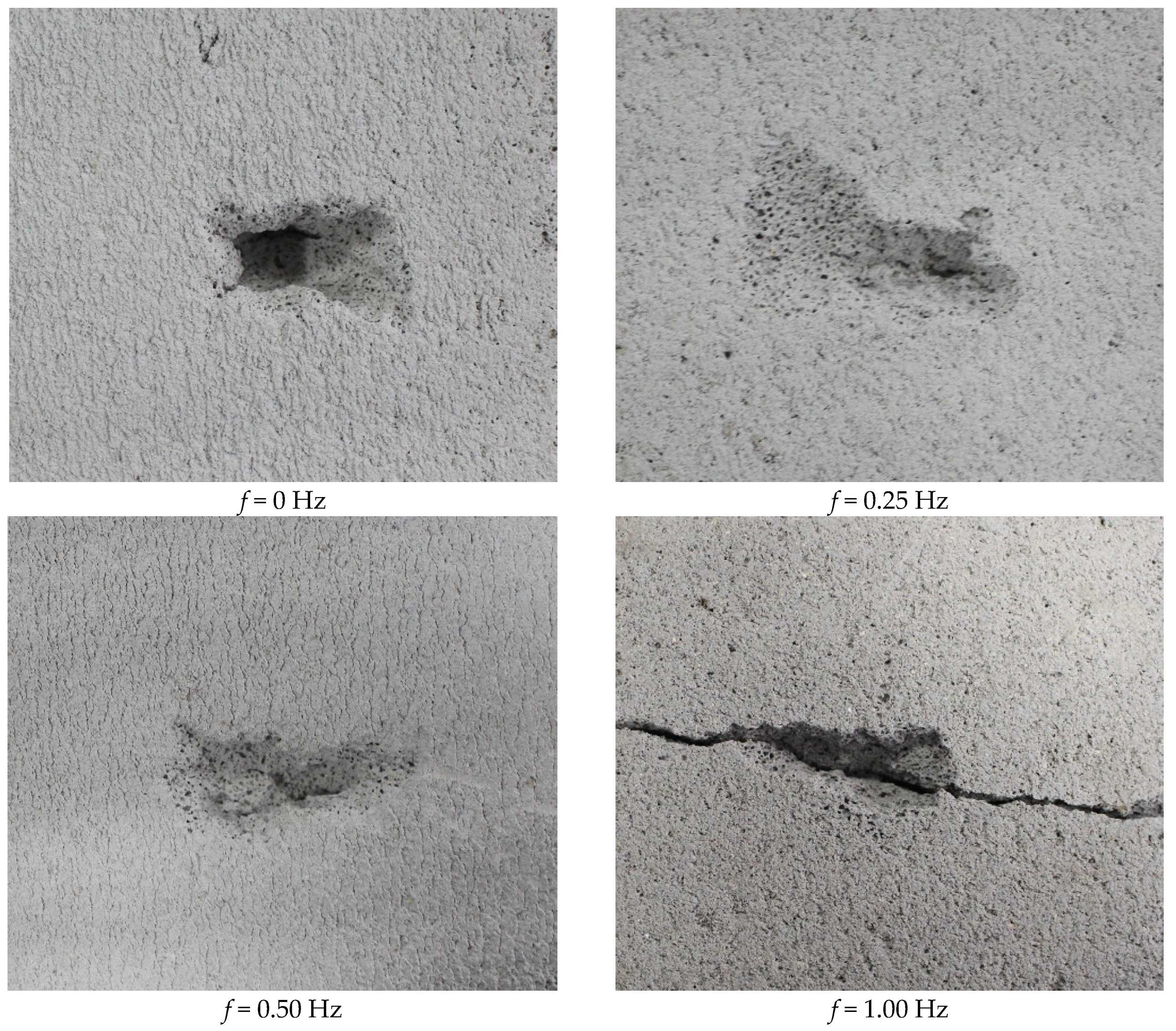
The erosion pattern of forced air excitation is presented in the Figure 21. As only one suction hole was open, the asymmetric flow was intensified with the forced air excitation. Jet deflection in the air-entry direction occurred, while little effect was observed in the other direction. As a result, “flat slot” shapes were observed on the specimens. With increasing forced frequency, stronger alternating shearing stress in the specimen occurred, and hence led to crack growth and crack branching of the specimen more easily.
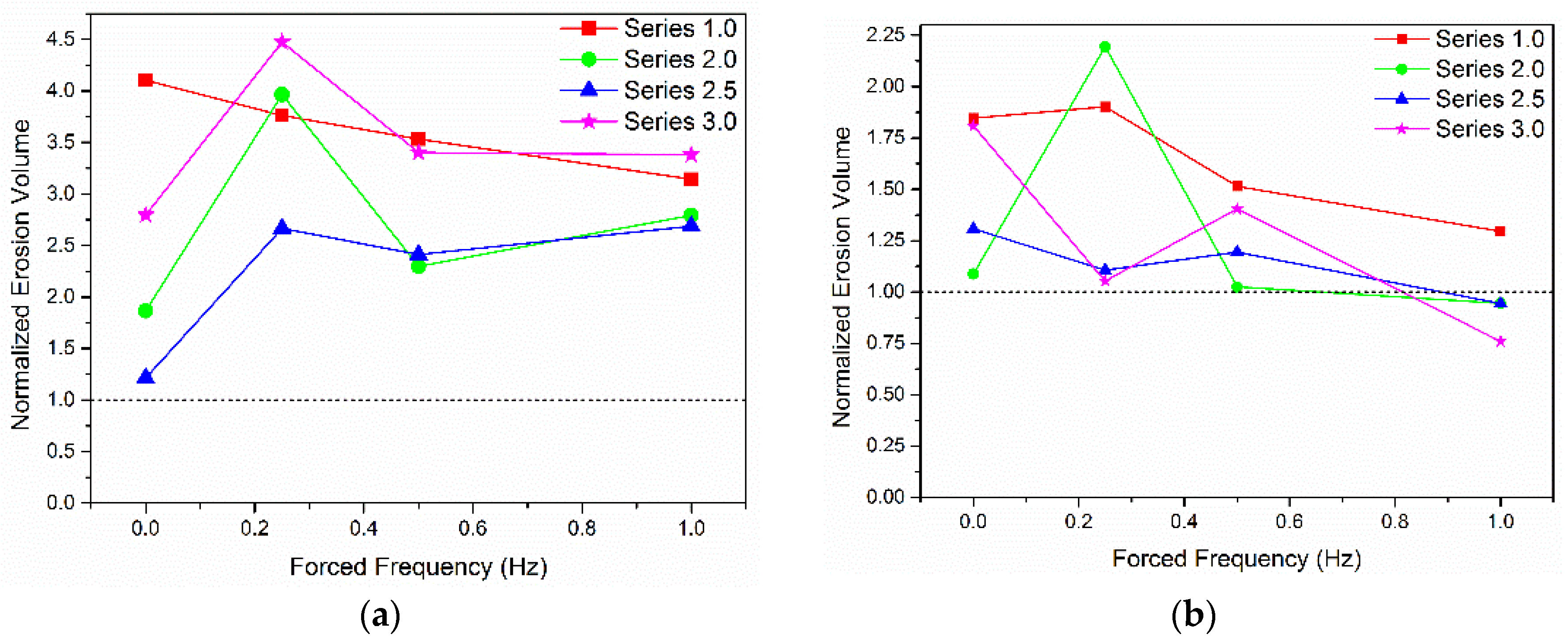
A significantly more effective erosion performance is observed in Figure 22 for the forced excitation frequency at 0.25 Hz, which was the closest to the oscillating frequency without air intake. It was necessary to select the forced frequency near to the fundamental frequency rather than the high frequency in order to achieve better performance. Besides, the volume of entrained air and the distribution of the air entry-path should also be considered. For the erosion volume, the series 3.0 achieved the maximum value, while series 2.0 achieved the maximum erosion area. Various combinations of the number and distributions of suction holes needed to be determined to achieve the expected goal (best erosion volume or largest erosion areas).
4. Conclusions
The better erosion performance of the resonating cavitation jet has long been acknowledged. In the present study, the LPHF nozzle, one of the resonating nozzles, was investigated from both experimental and numerical perspectives. Various inspiratory methods were adopted to achieve frequency modulation. Further erosion experiments showed that both entrained air and forced excitation are capable of achieving better erosion performance. Based on the present investigation, the main conclusions that can be drawn are:
- The Gas-Spring Theory was verified by both the experiment and the numerical simulation. The cavitation cluster dominated the oscillating frequency in the LPHF nozzle and the non-linear interaction between the cavitation cluster and acoustic modulation should also be considered. The global structure of the spectral distribution can be viewed as the result of non-linear interactions and modulation processes.
- The mechanism of frequency modulation was different with/without air intake. When no air was entrained, the dominant frequency increased linearly with the increasing pressure declines due to the decreasing accumulated time for the cavity cluster. For the LPHF nozzle with suction holes, the frequency of each inspiratory method did not vary monotonically with the pressure decrease.
- For the LPHF nozzle with suction holes, frequency modulation could be achieved in a wide range by simply changing the number and distribution of the open suction holes. The modulation range was dependent on the pressure decrease.
- For the forced exciting condition, the oscillating frequency was totally determined by the forced frequency of entrained air. With the increasing forced frequency, the mean volume of entrained air increased due to the fierce entraining and momentum transportation.
- The removal rate was improved with the entrained air. The erosion performance was affected by both the volume of entrained air and the distribution of the air entry-path. The best erosion performance was achieved at the frequency closest to the fundamental oscillation frequency. Thus, it is necessary to consider various combinations of the number and distributions of suction holes in order to achieve the expected goal.
The modulation of the jet has the great advantage of achieving an appreciable increase of material removal. In this study, a feasible method to improve the erosion performance of the LPHF nozzle has been proposed. Compared with a high-frequency water jet, it is much easier for the LPHF nozzle to achieve the desired frequency, as the oscillating frequency is quite low. Moreover, as the density of air is low, the wear problem can be ignored when compared with the use of a moving disk to interrupt the continuous water jet. This preliminary study could provide some suggestions for practical applications, and more accurate modulation should be achieved in future studies by considering the non-linear interaction.
Acknowledgments
This research is financially supported by the National Key Basic Research Program of China (No. 2014CB239203), the National Natural Science Foundation of China (No. 51474158) and the Program for New Century Excellent Talents in University of the Ministry of Education (Grant No: NCET-12-0424).
Author Contributions
Wenchuan Liu and Yongxiang Zhou conceived and designed the experiments; Wenchuan Liu and Mingxing Zhang performed the experiments; Wenchuan Liu performed the simulation, analyzed the data and wrote the paper; Yong Kang supervised the projects and the students with contributions to guide the research program. Xiaochuan Wang and Deng Li reviewed and read the final manuscript.
Conflicts of Interest
The authors declare no conflict of interest.
Nomenclature
| diameter | |
| length | |
| diameter of chamber hole | |
| convergent angle | |
| density | |
| time | |
| pressure | |
| viscosity | |
| mass transfer rate | |
| vapor volume fraction | |
| water volume fraction | |
| bubble radius | |
| saturation vapor pressure | |
| bubble number density | |
| turbulent kinetic energy | |
| turbulent eddy dissipation | |
| exponential coefficient | |
| cross section area | |
| volume of chamber | |
| f | oscillation frequency |
| circular frequency | |
| vapor phase volume | |
| adiabatic exponent of air |
Subscripts
| parameters of chamber | |
| property of gas | |
| property of water | |
| turbulence |
References
- Conn, A.F.; Johnson, V.E.; Liu, H.L.; Frederick, G.S. Evaluation of CAVIJET cavitating jets for deep-hole rock cutting. Geotherm. Energy 1981. [Google Scholar] [CrossRef]
- Chahine, G.L.; Conn, A.F.; Johnson, V.E.; Frederick, G.S. Cleaning and Cutting with Self-Resonating Pulsed Water Jets. In Proceedings of the U.S. Water Jet Conference, Rolla, MO, USA, 24–26 May 1983; pp. 167–176. [Google Scholar]
- Zhang, X.; Peng, J.; Ge, D.; Bo, K.; Yin, K.; Wu, D. Performance Study of a Fluidic Hammer Controlled by an Output-Fed Bistable Fluidic Oscillator. Appl. Sci. 2016, 6, 305. [Google Scholar] [CrossRef]
- Johnson, J.V.E.; Chahine, G.L.; Lindenmuth, W.T.; Conn, A.F.; Frederick, G.S.; Giac-Chino, J.G.J. Cavitating and Structered Jets for Mechanical Bits to Increase Drilling Rate. J. Energy Resour. Technol. 1982, 106, 289–294. [Google Scholar] [CrossRef]
- Johnson, V.E.; Chahine, G.L.; Lindenmuth, W.T.; Conn, A.F.; Frederick, G.S.; Giacchino, G.J. The Development of Structured Cavitating Jets for Deep Hole Bits. In Proceedings of the SPE Annual Technical Conference and Exhibition, New Orleans, LA, USA, 26–29 September 1982. [Google Scholar]
- Johnson, V.E.; Conn, A.F.; Lindenmuth, W.T.; Chahine, G.L.; Frederick, G.S. Self-Resonating Cavitating Jets. In Proceedings of the International Symposium on Jet Cutting Technology presented at the International Symposium on Jet Cutting Technology, Surrey, England, 16 January 1982; p. 16. [Google Scholar]
- Johnson, V.E.; Lindenmuth, W.T.; Conn, A.F.; Frederick, G.S. Feasibility study of tuned-resonator, pulsating cavitating water jet for deep-hole drilling. Petroleum 1981. [Google Scholar] [CrossRef]
- Morel, T. Experimental study of a jet-driven Helmholtz oscillator. J. Fluids Eng. 1978, 101, 383–390. [Google Scholar] [CrossRef]
- Liao, Z.F.; Tang, C.L. Theoretical analysis and experimental study of the selfexcited oscillation pulsed jet device. In Proceedings of the Fourth US Water Jet Conference, Berkeley, CA, USA, 26–28 August 1987. [Google Scholar]
- Rockwell, D.; Naudascher, E. Review—Self-Sustaining Oscillations of Flow Past Cavities. J. Fluids Eng. 1978, 100, 152–165. [Google Scholar] [CrossRef]
- Liao, Z.F.; Tang, C.L. Theoretical analysis and experimental study a self-excited oscillation pulsed jet device. J. China Coal Soc. 1989, 1, 90–100. [Google Scholar]
- Wang, X.M. Influence Factors Simulation Study of the Self-Excited Oscillation Pulsed Jet Device and Nozzle Structure Optimized Design. Ph.D. Thesis, Zhejiang University, Hangzhou, China, 2005. [Google Scholar]
- Kubota, A.; Kato, H.; Yamaguchi, H. A new modelling of cavitating flows: A numerical study of unsteady cavitation on a hydrofoil section. J. Fluid Mech. 1992, 240, 59–96. [Google Scholar] [CrossRef]
- Coutier-Delgosha, O.; Reboud, J.L.; Delannoy, Y. Numerical simulation of the unsteady behaviour of cavitating flows. Int. J. Numer. Methods Fluids 2003, 42, 527–548. [Google Scholar]
- Delannoy, Y. Two Phase Flow Approach in Unsteady Cavitation Modelling. In Proceedings of the Cavitation and Multiphase Flow Forum, Toronto, ON, Canada, 4–7 June 1990. [Google Scholar]
- Merkle, C.L.; Feng, J.; Buelow, P.E.O. Computational modeling of the dynamics of sheet cavitation. In Proceedings of the 3rd International Symposium on Cavitation, Grenoble, France, 7–10 April 1998. [Google Scholar]
- Kunz, R.F.; Boger, D.A.; Stinebring, D.R.; Chyczewski, T.S.; Lindau, J.W.; Gibeling, H.J.; Venkateswaran, S.; Govindan, T.R. A preconditioned Navier–Stokes method for two-phase flows with application to cavitation prediction. Comput. Fluids 2000, 29, 849–875. [Google Scholar] [CrossRef]
- Habil, S.I. Physical and Numerical Modeling of Unsteady Cavitation Dynamics. In Proceedings of the International Conference on Multiphase Flow (ICMF-2001), New Orleans, LA, USA, 27 May–1 June 2001. [Google Scholar]
- Singhal, A.K.; Athavale, M.M.; Li, H.; Jiang, Y. Mathematical Basis and Validation of the Full Cavitation Model. J. Fluids Eng. 2002, 124, 617–624. [Google Scholar] [CrossRef]
- Ducoin, A.; Huang, B.; Yin, L.Y. Numerical Modeling of Unsteady Cavitating Flows around a Stationary Hydrofoil. Int. J. Rotat. Mach. 2012, 2012. [Google Scholar] [CrossRef]
- Frikha, S.; Coutierdelgosha, O.; Astolfi, J.A. Influence of the Cavitation Model on the Simulation of Cloud Cavitation on 2D Foil Section. Int. J. Rotat. Mach. 2014, 2008, 498–499. [Google Scholar] [CrossRef] [Green Version]
- Morgut, M.; Nobile, E.; Bilu, I. Comparison of mass transfer models for the numerical prediction of sheet cavitation around a hydrofoil. Int. J. Multiph. Flow 2011, 37, 620–626. [Google Scholar] [CrossRef]
- Senocak, I.; Wei, S. Interfacial dynamics-based modelling of turbulent cavitating flows, Part-1: Model development and steady-state computations. Front. Public Health 2004, 2, 141. [Google Scholar] [CrossRef]
- Goncalvès, E.; Charrière, B. Modelling for isothermal cavitation with a four-equation model. Int. J. Multiph. Flow 2014, 59, 54–72. [Google Scholar] [CrossRef] [Green Version]
- Momber, A.W. Concrete failure due to air-water jet impingement. J. Mater. Sci. 2000, 35, 2785–2789. [Google Scholar] [CrossRef]
- Kollé, J.J. Coiled tubing drilling with supercritical carbon dioxide. In Proceedings of the SPE/CIM International Conference on Horizontal Well Technology, Calgary, AB, Canada, 6–8 November 2000. [Google Scholar]
- Hu, D.; Li, X.H.; Tang, C.L.; Kang, Y. Analytical and experimental investigations of the pulsed air–water jet. J. Fluids Struct. 2014, 54, 88–102. [Google Scholar] [CrossRef]
- Huang, N.E.; Shen, Z.; Long, S.R.; Wu, M.C.; Shih, H.H.; Zheng, Q.; Yen, N.C.; Chi, C.T.; Liu, H.H. The Empirical Mode Decomposition and the Hilbert Spectrum for Nonlinear and Non-stationary Time Series Analysis. Proc. R. Soc. Lond. A 1998, 454, 903–995. [Google Scholar] [CrossRef]
- Wang, J. Study on the Mechanism of Low-Frequency Self-Excited Pulse Jet Flow and the Frequency Modulation. Ph.D. Thesis, Wuhan University, Wuhan, China, 2016. [Google Scholar]
- Zhou, Y.X. Experimental Study about Self-Excited Pulsed Suction Jet. Master’s Thesis, Wuhan University, Wuhan, China, 2016, unpublished. [Google Scholar]
- Reboud, J.L.; Stutz, B.; Coutier, O. Two-phase flow structure of cavitation: Experiment and modeling of unsteady effects. In Proceedings of the 3rd International Symposium on Cavitation CAV1998, Grenoble, France, 7–10 April 1998. [Google Scholar]
- Cheng, H.; Long, X.; Ji, B.; Zhu, Y.; Zhou, J. Numerical investigation of unsteady cavitating turbulent flows around twisted hydrofoil from the Lagrangian viewpoint. J. Hydrodyn. 2016, 28, 709–712. [Google Scholar] [CrossRef]
- Coutier-Delgosha, O.; Fortes-Patella, R.; Reboud, J.L. Evaluation of the Turbulence Model Influence on the Numerical Simulations of Unsteady Cavitation. In Proceedings of the ASME FEDSM, New Orleans, LA, USA, 29 May–1 June 2001; pp. 38–45. [Google Scholar]
- Decaix, J.; Goncalvès, E. Compressible effects modeling in turbulent cavitating flows. Eur. J. Mech. 2013, 39, 11–31. [Google Scholar] [CrossRef]
- Long, X.P.; Liu, Q.; Ji, B.; Lu, Y.Y. Numerical investigation of two typical cavitation shedding dynamics flow in liquid hydrogen with thermodynamic effects. Int. J. Heat Mass Transf. 2017, 879–893. [Google Scholar] [CrossRef]
- Basley, J.; Pastur, L.R.; Lusseyran, F.; Faure, T.M.; Delprat, N. Experimental investigation of global structures in an incompressible cavity flow using time-resolved PIV. Exp. Fluids 2011, 50, 905–918. [Google Scholar] [CrossRef]
- Delprat, N. Rossiter’s formula: A simple spectral model for a complex amplitude modulation process. Phys. Fluids 2006, 18, 152. [Google Scholar] [CrossRef]
- Delprat, N. Low-frequency components and modulation processes in compressible cavity flows. J. Sound Vib. 2010, 329, 4797–4809. [Google Scholar] [CrossRef]
- Knisely, C.; Rockwell, D. Self-sustained low-frequency components in an impinging shear layer. J. Mech. 2006, 116, 157–186. [Google Scholar] [CrossRef]
- Lucas, M.; Rockwell, D. Self-excited jet—Upstream modulation and multiple frequencies. J. Fluid Mech. 2006, 147, 333–352. [Google Scholar] [CrossRef]
- Miksad, R.W.; Jones, F.L.; Powers, E.J. Measurements of nonlinear interactions during natural transition of a symmetric wake. Phys. Fluids 1983, 26, 1402–1409. [Google Scholar] [CrossRef]
- Luo, Z.C. Fluidic Networks; China Machine Press: Beijing, China, 1988. [Google Scholar]
- Wright, M.M.; Epps, B.; Dropkin, A.; Truscott, T.T. Cavitation of a submerged jet. Exp. Fluids 2013, 54, 1541. [Google Scholar] [CrossRef]
Figure 1.
Schematic diagram of the 120° -impinging edge Helmholtz nozzle.
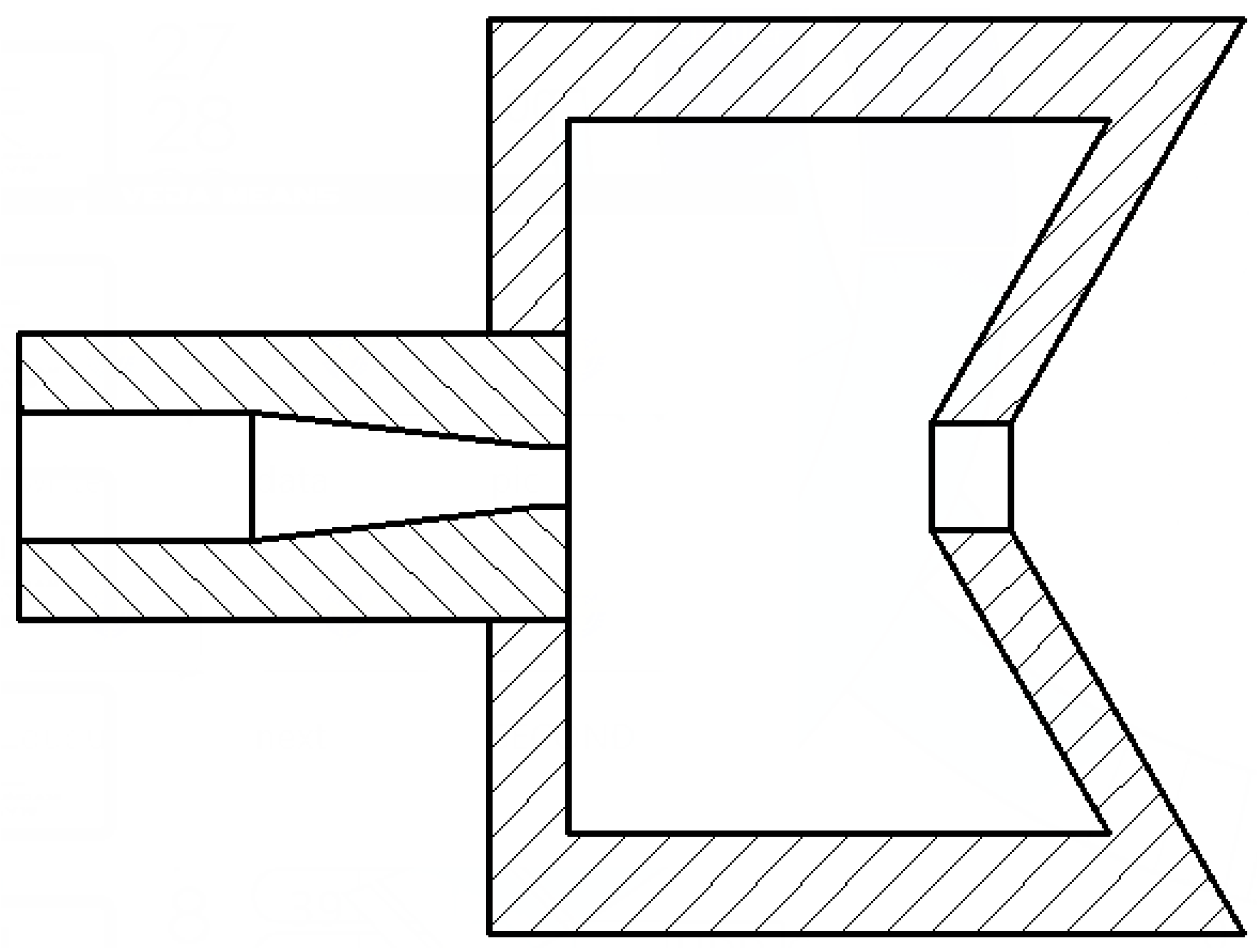
Figure 2.
Schematic diagram of the experimental setup.

Figure 3.
Material testing machine.

Figure 4.
The electronic balance.
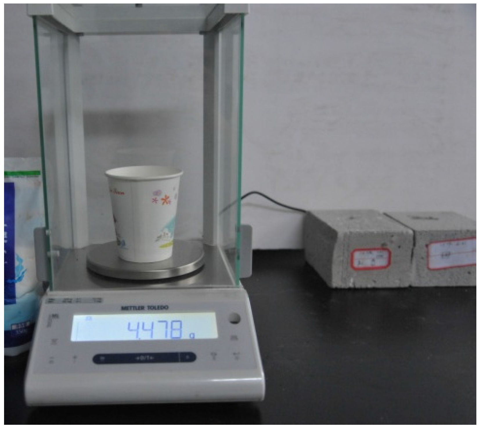
Figure 5.
Measuring method of erosion area.
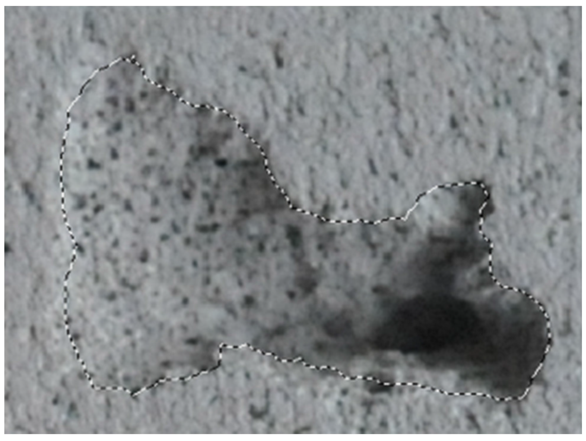
Figure 6.
Profiles and photos of the three fittings.
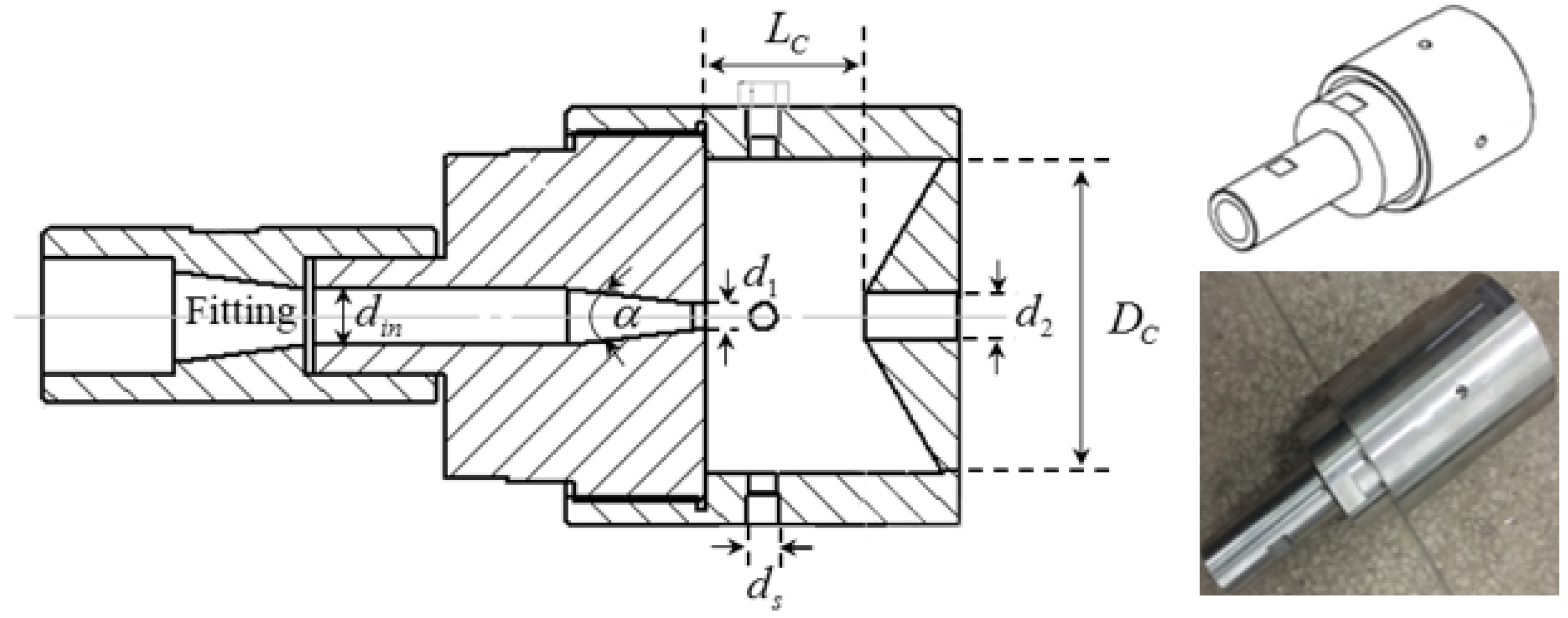
Figure 7.
Description of suction hole distribution.
Figure 8.
2D computational axisymmetric domain and boundary conditions.
Figure 9.
The distribution of monitor lines.
Figure 10.
Average streamwise velocity profiles.
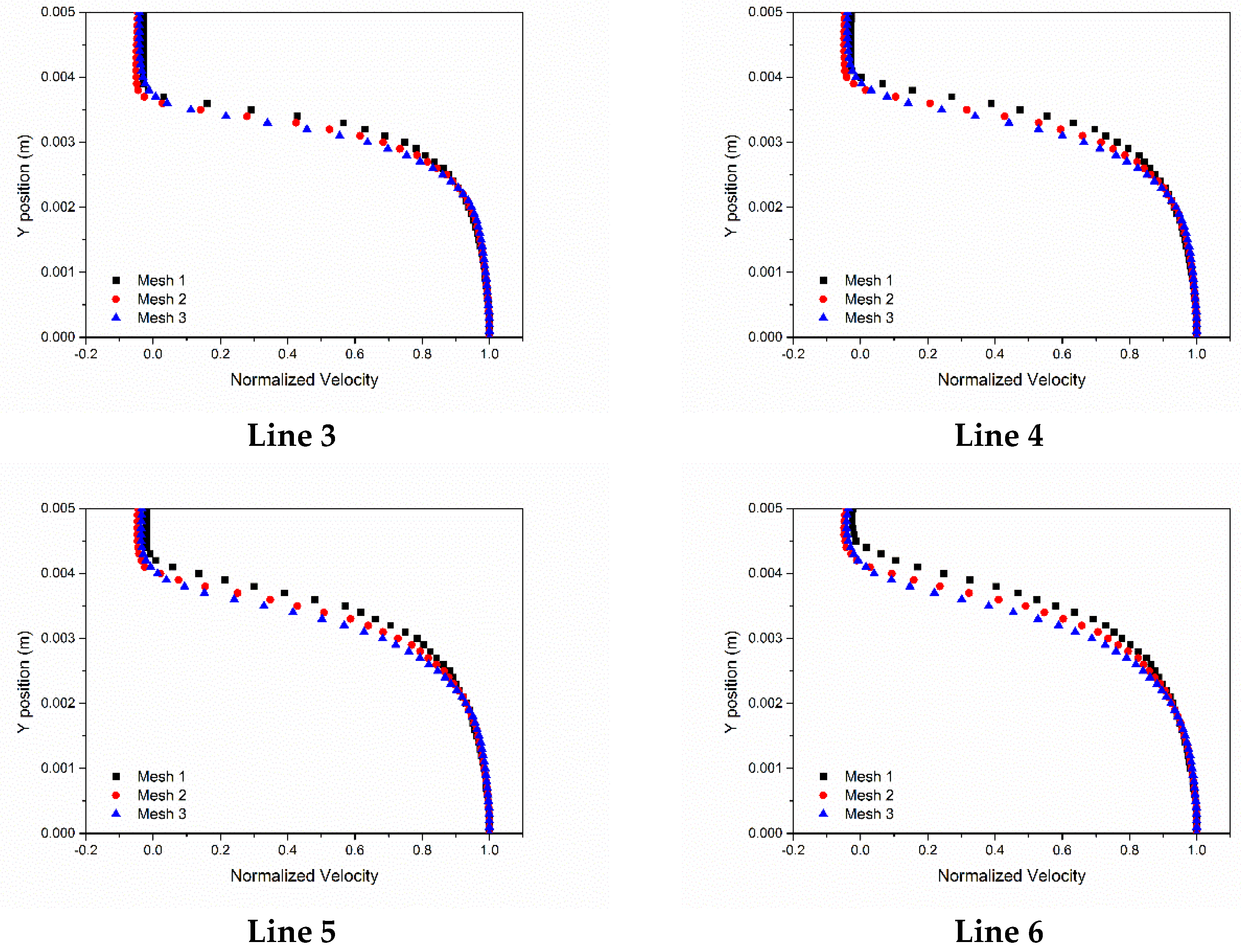
Figure 11.
Pressure signal and marginal spectrum of the chamber pressure.
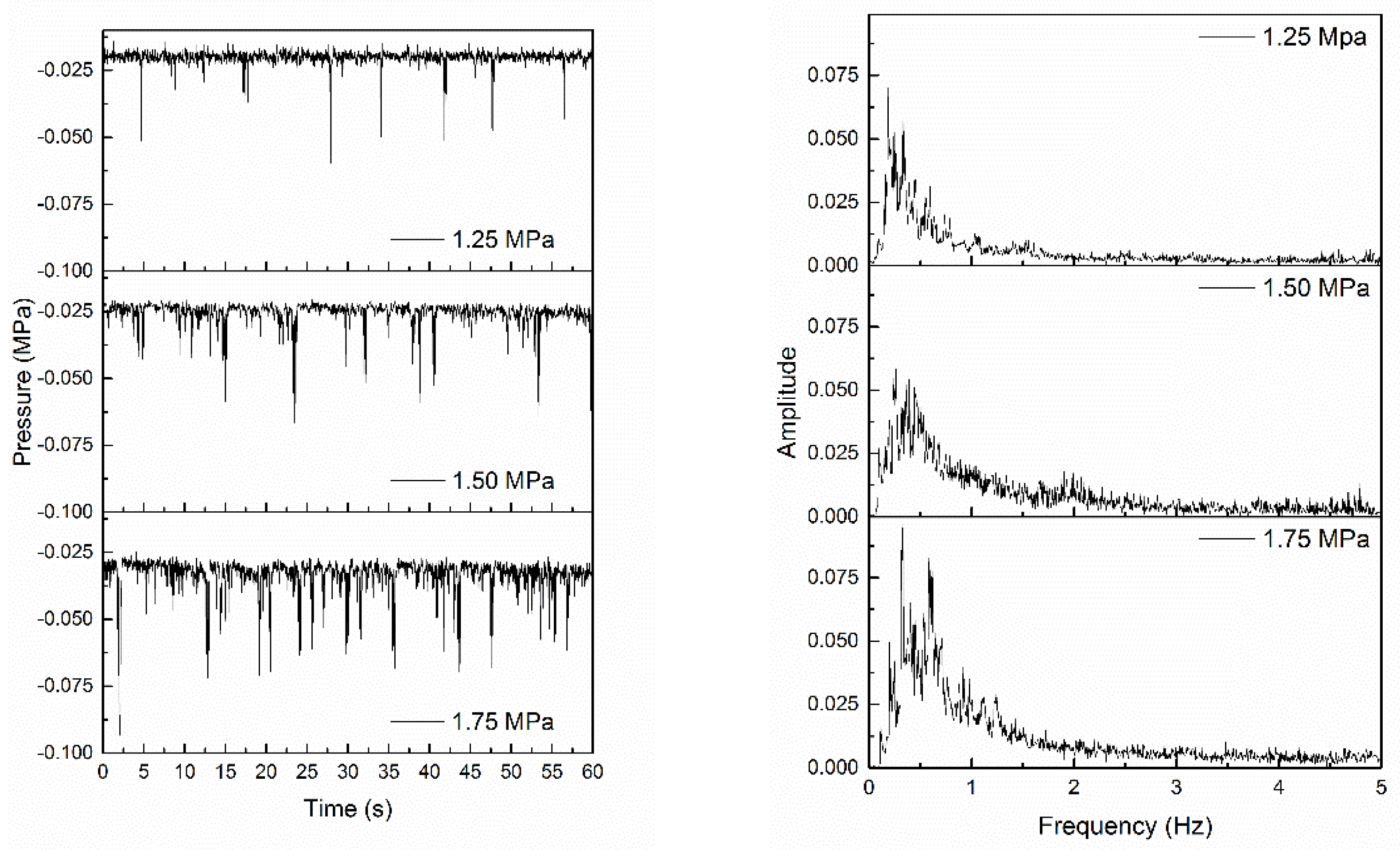
Figure 12.
Instantaneous energy density of various pressure drops.
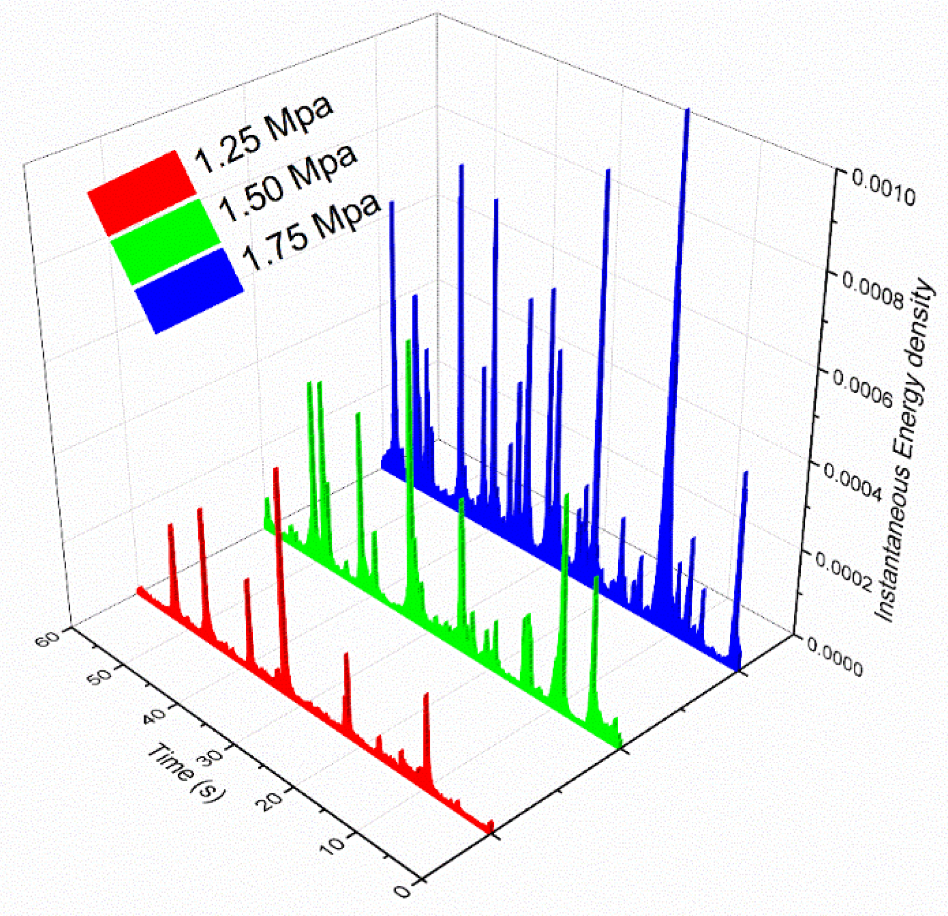
Figure 13.
Marginal spectrum of vapor volume.

Figure 14.
Time evolution of cavity volume during one typical cycle.
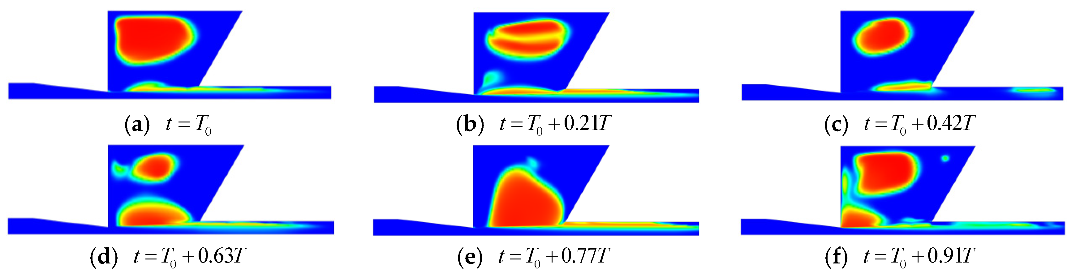
Figure 15.
Chamber pressure signal under various suction series.
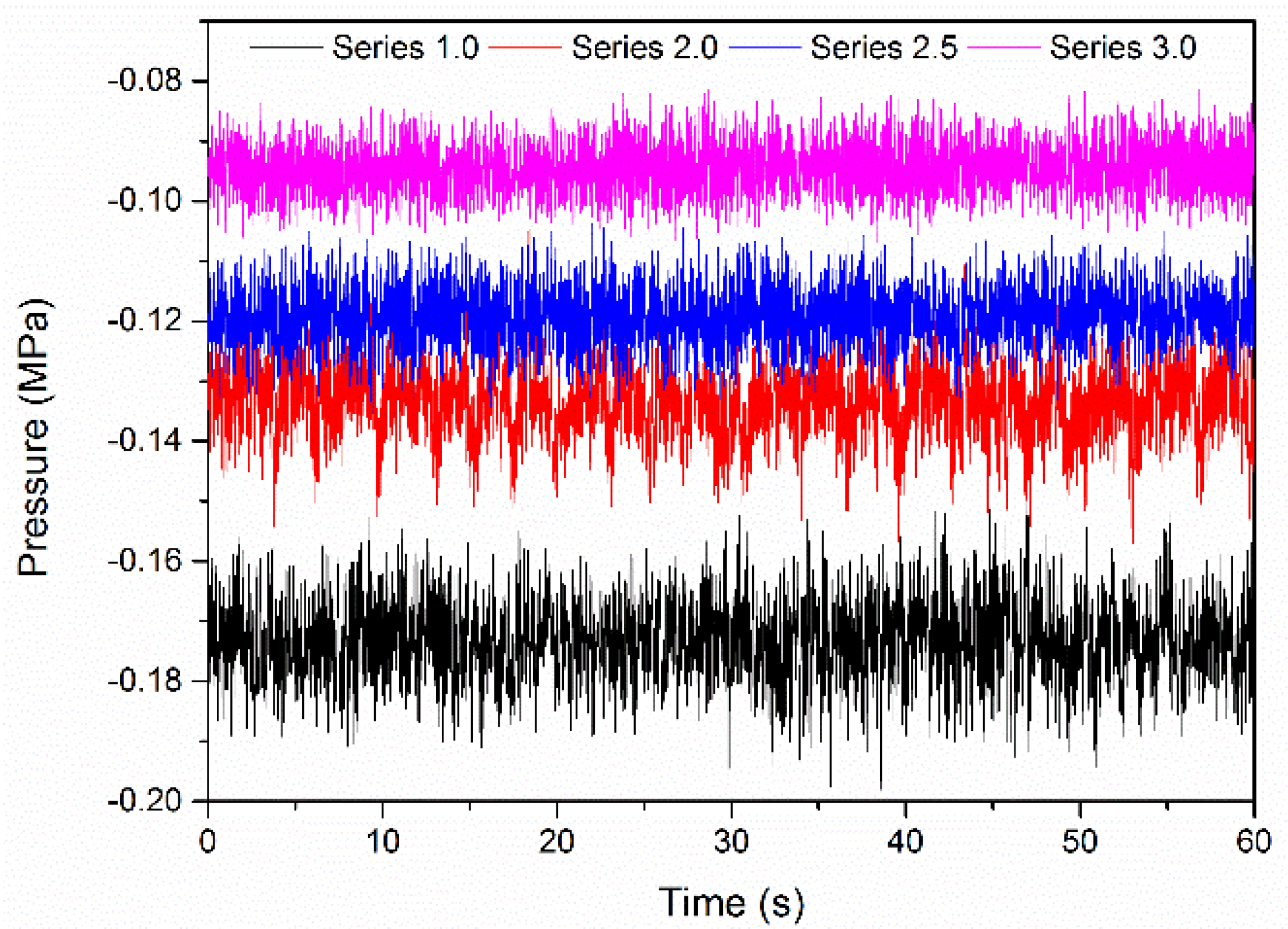
Figure 16.
Marginal spectrum.

Figure 17.
Dominant frequency in the frequency modulation.

Figure 18.
The erosion pattern of specimens.

Figure 19.
The erosion performance under various suction series.

Figure 20.
Time-resolved signals under forced excitation: (a) chamber pressure and (b) volume of entrained air.
Figure 20.
Time-resolved signals under forced excitation: (a) chamber pressure and (b) volume of entrained air.

Figure 21.
The erosion pattern of specimens under forced excitation (Series 1.0).

Figure 22.
The erosion performance under forced excitation: (a) normalized volume; (b) normalized area.
Figure 22.
The erosion performance under forced excitation: (a) normalized volume; (b) normalized area.

Table 1.
Experimental condition.
| Suction Series | Pressure Drop | Exciting Frequency |
|---|---|---|
| 0.0 | 1.25 MPa | 0 Hz |
| 1.0 | 1.50 MPa | 0.25 Hz |
| 2.0 | 1.75 MPa | 0.50 Hz |
| 2.5 | 1.00 Hz | |
| 3.0 |
© 2017 by the authors. Licensee MDPI, Basel, Switzerland. This article is an open access article distributed under the terms and conditions of the Creative Commons Attribution (CC BY) license (http://creativecommons.org/licenses/by/4.0/).
Share and Cite
MDPI and ACS Style
Liu, W.; Kang, Y.; Zhang, M.; Zhou, Y.; Wang, X.; Li, D. Frequency Modulation and Erosion Performance of a Self-Resonating Jet. Appl. Sci. 2017, 7, 932. https://doi.org/10.3390/app7090932
AMA Style
Liu W, Kang Y, Zhang M, Zhou Y, Wang X, Li D. Frequency Modulation and Erosion Performance of a Self-Resonating Jet. Applied Sciences. 2017; 7(9):932. https://doi.org/10.3390/app7090932
Chicago/Turabian StyleLiu, Wenchuan, Yong Kang, Mingxing Zhang, Yongxiang Zhou, Xiaochuan Wang, and Deng Li. 2017. "Frequency Modulation and Erosion Performance of a Self-Resonating Jet" Applied Sciences 7, no. 9: 932. https://doi.org/10.3390/app7090932
Note that from the first issue of 2016, this journal uses article numbers instead of page numbers. See further details here.