A New Method for Analysing the Pressure Response Delay in a Pneumatic Brake System Caused by the Influence of Transmission Pipes


1
School of Mechanical and Electronic Engineering, Wuhan University of Technology, Wuhan 430070, China
2
Laboratory for FIRST, Tokyo Institute of Technology, Yokohama 226-8503, Japan
*
Author to whom correspondence should be addressed.
Appl. Sci. 2017, 7(9), 941; https://doi.org/10.3390/app7090941
Submission received: 29 July 2017
/
Revised: 2 September 2017
/
Accepted: 9 September 2017
/
Published: 13 September 2017
(This article belongs to the Special Issue Power Transmission and Control in Power and Vehicle Machineries)
Abstract
:This study aims to propose an analysis method for resolving the pressure response of a pneumatic brake circuit considering the effect of a transmission pipe. Pneumatic brake systems (PBS) are widely used in commercial vehicles. The pressure response characteristic of the PBS is the key factor affecting braking performance. By using the thermodynamics of a variable-quality system, the pressure response model of the brake chamber is established, which includes the dynamic model of the pipe considering the unsteady friction and heat transfer. The partial-differential control equations of pipe are solved by introducing the constrained interpolation profile (CIP) method, and a virtual chamber model is proposed to set the boundary condition so as to solve the pressure response in the brake chamber simultaneously. Thus, the regularity of the brake pressure response is obtained by considering the influence of the pipe. Lastly, the model is verified experimentally. The present study indicates that the main factors that affect the pressure response delay are the pipe length and the combination forms of the sonic conductances of the orifices inlet and outlet. Furthermore, it helps to verify that the CIP method is an effective way of solving the pressure response of a brake circuit because of its high accuracy. The present study serves as a foundation for the design and analysis of a PBS.
1. Introduction
The brake system is the key component guaranteeing the safety of vehicles, and its performance affects driving safety, braking stability and passenger comfort. At present, pneumatic brake systems (PBSs) are widely used in buses and heavy trucks for their cleanliness, simple structure and high reliability. However, many nonlinear factors, including the compressibility of air and the unsteady characteristics of braking, make it difficult to calculate the characteristics of PBSs accurately. Hence, their design is based mostly on experience or experiments [1], which harms their efficiency and increases their maintenance cost. Therefore, researchers are always looking for ways to enhance the performance of PBSs [2,3]. An electro-pneumatic proportional valve was proposed to replace the antilock brake system so as to control the brake pressure more accurately [4], but it has been rarely used in vehicles because of its high cost. Europe and America have proposed the mandatory installation of emergency brake systems on vehicles for active safety [5], but their spread in Asian countries has been slow because of cost and problems with the technology. Consequently, if the performance of PBSs could be enhanced by optimising their control algorithm or improving the accuracy of their analysis model, this would broaden their application prospects and avoid spiralling hardware costs.
When the driver treads on the brake pedal to decelerate or stop a vehicle, there is time consumption that includes the response time of the driver, the transmission time of force and signals, and the action time of the actuator. All of these factors cause brake hysteresis more often when compared to the brake expectation, and the hysteresis is the response delay of the brake system. The response time delay consists of the delay of pedal valve, pneumatic brake circuit, actuator, and control networks. Wang et al. [6] had proved that a pipe in a pneumatic brake system account for 30% of the overall time delay by experiment but without theoretical analysis. Therefore, the time delay caused by a pipe is an important part of the delay of a pneumatic brake circuit. In this paper, we mainly focused on the time delay caused by the influence of a pipe but did not study the other factors. Because of the time delay of the pneumatic brake system, the time delay will cause the longitudinal or lateral braking distance deviation [7]. Especially, for the emergency braking condition, a tiny deviation of braking distance may lead to vehicle crash and the death of a human. Table 1 gives the braking distance with different time delays referred to in [8]. It is obvious that the brake distance increases considerably when the time delay increases. Thus, ISO7346 and GB/T7258 clearly define the range of time delay to guarantee safe driving. Therefore, decreasing the response time delay or identifying the time delay and controlling it with proper control methods are effective ways to decrease the brake distance and increase driving safety.
At present, the low cost and high efficiency of computer simulation means that it is the main way of studying the performance of brake systems. For example, He et al. [9,10,11] used AMESim, SIMULINK and MWorks to establish a model of a brake system and study its pressure response characteristics. However, the algorithms of these commercial software packages are closed, which makes it difficult to use them to develop brake systems with different requirements. Meanwhile, simulations using such software are based on time sampling, which makes it difficult to tackle problems that are both temporally and spatially dependent. Thus, the distributed-parameter components, such as the pipe, are equivalent by restriction or capacity-restriction (it sacrifices the accuracy artificially). Furthermore, adiabatic and isothermal models [9,10] are mostly used for modelling the brake chamber, which simplifies the analysis but also reduces its accuracy. The brake chamber is a particular air cylinder, and Tokashiki et al. [12] have shown that the pipe affects the dynamic characteristics of this cylinder via the temperature changes caused by the pipe. Qin [7] demonstrated experimentally the existence of a pipe led time delay in a PBS, and proposed compensating for it in the design of the control system. However, that approach is not a universal method because it lacks a theoretical basis. Therefore, it is important to consider the influence of the pipe so as to calculate the brake force response accurately.
To calculate the pressure response in the pipe, it is necessary to solve the partial-differential equations (PDEs) represented by the continuity, kinematic and energy equations. Zielke [13] first solved these equations by the method of characteristics considering the friction. However, he neglected advection and temperature change, so his approach is suitable only for low-pressure, low-speed problems. In addition, Zielke’s method has to solve a convolution integral repeatedly, which is inefficient. Kitagawa et al. [14] then proposed an optimised method in which the convolution integral is replaced by an exponential function, which improves the efficiency markedly. Hashimoto et al. [15] proposed a grid differential scheme to calculate the large pressure surge in the pipe, but that approach is only first-order accurate and the time step must be sufficiently small to avoid divergence. Wei et al. [16,17] also used the method of characteristics to solve the pressure response in the brake circuit of a train. However, it is complex to solve the characteristics curve and the time step must be strictly equal to the spatial step divided by the speed, which are restrictions that make such an approach difficult to apply universally. The key difficulty in calculating the pressure response in the pipe is to solve the PDE control equations accurately. Yabe et al. [18] and Takewaki et al. [19] proposed the constrained interpolation profile (CIP) method with third-order accuracy, which is good for solving hyperbolic PDEs. The CIP method uses a cubic interpolation to calculate the values between grid nodes, and has obtained good results in many applications. For example, it has been used for weather forecasting and for simulating dam failures and hull shock waves [20,21], all cases in which natural phenomena were predicted accurately.
Through the analysis above, the deficiencies in previous studies of PBSs can be summarised as follows. Either the influence of the pipe was neglected or the pipe was replaced by a simple restriction, both of which approaches reduce the accuracy. Also, the conventional methods used for solving the PDEs were either of low accuracy or were inefficient. Furthermore, heat exchange between the system and its surroundings was neglected, which also reduces the accuracy. In contrast, in the present study, the accurate CIP method is introduced and the heat exchange is considered comprehensively. We couple the models of the pipe and the brake chamber and solve them simultaneously, bringing regularity to the influence of the pipe parameters on the response of the brake pressure. The present study provides a good reference for the design and analysis of a PBS.
2. Modelling the Brake Pressure Response
A typical pneumatic brake circuit is shown in Figure 1. It consists of a compressor, an air filter, a compressed-air reservoir, a pedal valve, pipes and four brake chambers, and so on. This pneumatic brake circuit consists of four subcircuits, which are front brake circuit, rear brake control circuit, rear brake circuit, and parking brake circuit. When the driver treads on the pedal, the pedal valve opens and the compressed air flows into the front and rear brake chambers through the brake control valve and pipe. The rear brake chamber is relatively farther from the air tank, and then a relay valve is used to decrease the time delay. In these four subcircuits, the similarity is that all of the subcircuits use long pipes to transmit the air. Moreover, the time delay of a pipe is the key point that should be first solved. The operation pressure is generally 0.6–0.8 MPa for a pneumatic brake system, and the diameter of a transmission pipe is 6–16 mm. When analysing the brake circuit, we can study the subcircuit one by one. In this study, we mainly focused on the calculation method of the time delay caused by a transmission pipe; thus, we will simplify the system into one circuit to describe the modelling method clearly.
Although the brake control valve has a complex internal structure, the air flows through it quickly and its volume is small, so it can be thought of as lumped parameter components. The main effects of the brake control valve on the braking process are its flow-rate characteristics and the time delay of the mechanism. Therefore, when modelling the brake system, the brake control valve can be dealt with as an orifice [22]. For a pneumatic transmission circuit, the flow-rate characteristics of the circuit depend mainly on the smallest component and its upstream components; the downstream components have little effect [23]. In this paper, we mainly focused on the modelling and solving method of the pipe. Conversely, compared with the pipe, the sonic conductance of the control valve is smaller. Therefore, the valve can be considered as an orifice with a constant effective area.
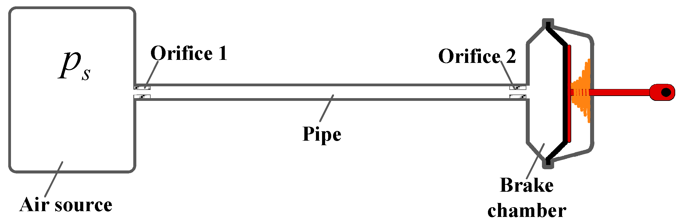
Thus, the simple circuit shown in Figure 2 is adopted as the research object in the present paper, which is composed of an air source, two orifices, a pipe, and a brake chamber. In the actual application, orifice 1 depends on the control valve and orifice 2 is the inlet orifice of the brake chamber. According to ISO6358 [24], the flow-rate characteristics of the components can be measured by the isothermal chamber (ITC) discharge method, and the time delay of the brake control valve can be obtained according to ISO19973 [25]. The resultant flow-rate characteristics of the components in a circuit can be calculated by referring to [23,26].
- (a)
- The working fluid (air) of the system follows all ideal gas laws;
- (b)
- There is no leakage from the fittings or the brake chamber;
- (c)
- The airflow in the pipe is a one-dimensional flow, and the parameters in each section are uniform.
2.1. Flow-Rate Characteristics of the Orifice
According to ISO6358, the sonic conductance C and the critical pressure ratio b are used as the main parameters to describe the flow-rate characteristics [24]. Thus, if we know the flow-rate characteristics of an orifice, the flow-rate output from the tank or the input to the brake chamber can be obtained according to the definition of the flow-rate characteristics. However, we will use numerical computation in the following discussion, so we are introducing a corrected formula proposed by Kassa [29] so as to avoid numerical divergence if the step size becomes too large. Hence, the mass flow rate of air through an orifice can be given as
where k1 is the linear gain obtained by
2.2. Modelling the Pipe
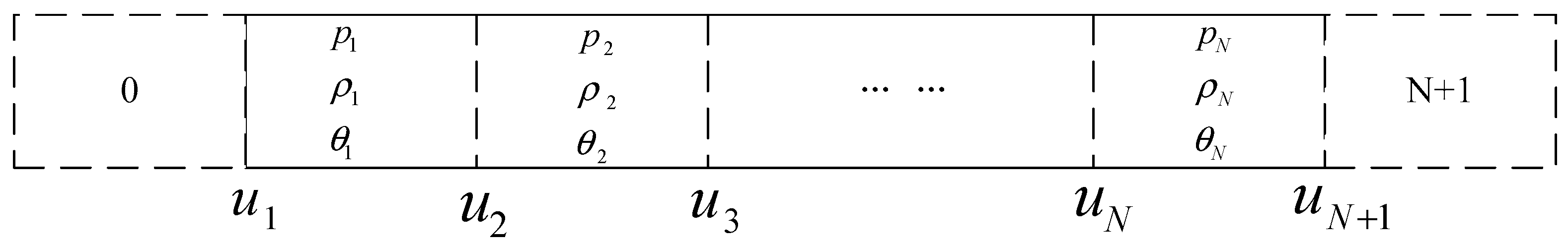
In a PBS, the pipe is the medium for air transmission and is the key component that causes time delays in the system. The length of the vehicle body could be up to 20 m for a large bus or a truck, so it is necessary to consider the influence of the pipe when it transmits pressure. The pipe is sufficiently long for both the pressure and temperature to be spatially and temporally dependent, so we deal with the pipe as a distributed-parameter component to enhance the analysis accuracy. Figure 3 shows the analysis model used for the pipe, in which each element in the dashed line is the control volume, and it is also the grid we will use in the next section.
The diameters of the pipes commonly used in pneumatic brake circuits are in the range 6–16 mm, which is very small compared with the pipe length. Hence, the flow in the pipe can be thought of as being a one-dimensional flow. According to gas dynamics, the air in the control volume satisfies the conservation of mass, momentum, and energy [30]. So, the control volume can be described by the control equations as follows:
To enhance the model accuracy, in Equations (3)–(5), we consider the friction loss and heat exchange, respectively, in terms of a friction loss coefficient λ and the heat convection q between the control volume and its surroundings. Coefficient λ is a function of the Reynolds number according to the flow regime and is expressed as follows:
Re is the Reynolds number given by , where u is the gas velocity, D is the diameter of pipe, and is kinematic viscosity.
And then the heat exchange q is given by
where and Pr is the Prandtl number, which is equal to 0.72 for air.
By using Equations (3)–(7), we comprehensively consider the factors related to nonlinear effects, whereupon the pressure, density, and temperature in each control volume can be solved accurately. Furthermore, we can obtain the regularity for these physical quantities that change temporally and spatially. However, it is difficult to solve these hyperbolic PDEs analytically because they include many nonlinear factors, such as heat exchange and friction. The methods used most commonly to solve PDEs are up-wind difference schemes, central difference schemes, and the Lax–Wendroff method [31]. However, these all deliver only either first-order or second-order accuracy, and their stability is very poor for a large pressure surge. Thus, to enhance the accuracy and stability, we introduce the CIP method with its third-order accuracy; the details will be explained later.
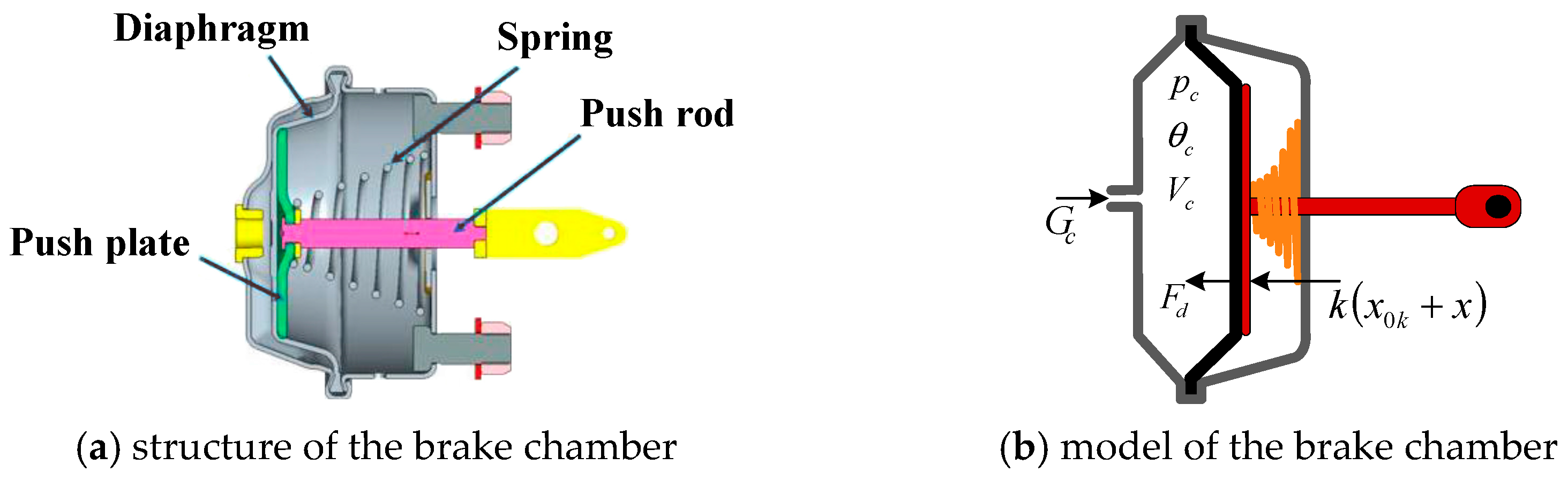
2.3. Modelling the Brake Chamber
Figure 4a shows the structure of the brake chamber, which consists of a diaphragm, a push plate, a push rod, and a spring, thereby forming two chambers. When braking is applied, the rod-less chamber is charged, the air expands to push the piston and push rod, and then the rod chamber is compressed. However, there are four holes in the rod chamber with diameters of 6–8 mm so that the air can be discharged to the atmosphere as quickly as possible, and this means that there is no back pressure in the rod chamber. Thus, we need only consider the rod-less chamber when modelling the brake chamber.
The main parameters are shown in Figure 4b. By differentiating the gas state equation with respect to time, the pressure response in the rod-less chamber is obtained as
To improve the accuracy of the model, we consider here the heat exchange in the brake chamber. Thus, according to the first law of thermodynamics, the energy flow in or out of the chamber always satisfies
where U is the internal energy, H is the enthalpy that flows in the chamber, W is the work done by the rod, and Q is the heat exchanged between the inner chamber and the surroundings through the wall, which can be expressed as follows according to Newton’s law of cooling:
The heat-exchange coefficient h can be measured using the stop method [32]. However, it changes during the charging process, so we adopt an average value here of h = 20. In addition, the model is adiabatic for h = 0, tending to isothermal has h → ∞.
By differentiating Equation (9) with respect to time and combining it with the equations , and the Mayer equation cp−cv = R, we obtain the temperature response as
The volume Vc of the diaphragm changes as that of a cone rather than a cylinder, and is given approximately by
The force on the piston is shown diagrammatically in Figure 4b, from which the kinematic equation of the push rod can be obtained as follows according to Newton’s second law of motion:
where is the effective loaded area, which changes during the stroke of the piston [33] and is expressed as
In Equation (13), Fd is the deforming force on the diaphragm, which also changes during the stroke and is expressed as
Through the three models established above, we obtain an analytical model for the brake pressure response. The method for obtaining solutions to this model is discussed in detail in Section 3.
3. Simulations and Experiments on Brake Pressure Response
3.1. Solving the Pipe Control Equations
3.1.1. CIP Method
First proposed by Yabe [18,19] in the 1980s, the CIP method is an effective way to solve hyperbolic PDEs. It uses the function value and its derivative on a spatial grid, and then a cubic interpolation is constructed so that the values between nodes can be solved inversely. The CIP method is an explicit scheme of numerical computation with third-order accuracy [20]. Equation (16) is a typical hyperbolic PDE:
If the speed u is positive and constant, the analytical solution is . This means that the value of a node at the next time step can be obtained from the current one; however, the location is not on the node but is shifted by an amount from it. As we know, is located between two nodes, so we need to solve the value at by interpolation. The highly accurate interpolation expression proposed by Yabe is given as
The coefficients in Equation (17) can be obtained using Equations (18)–(21):
when , , ; and if , , .
where ξ = −uiΔt.
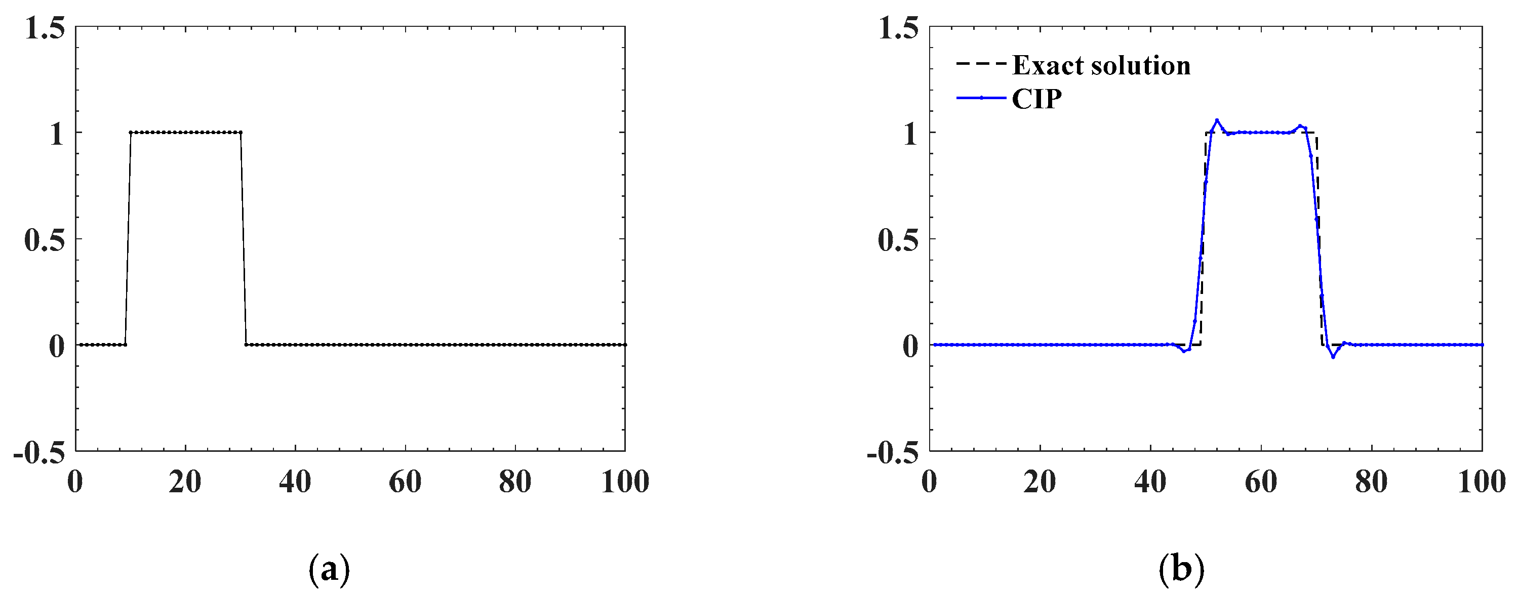
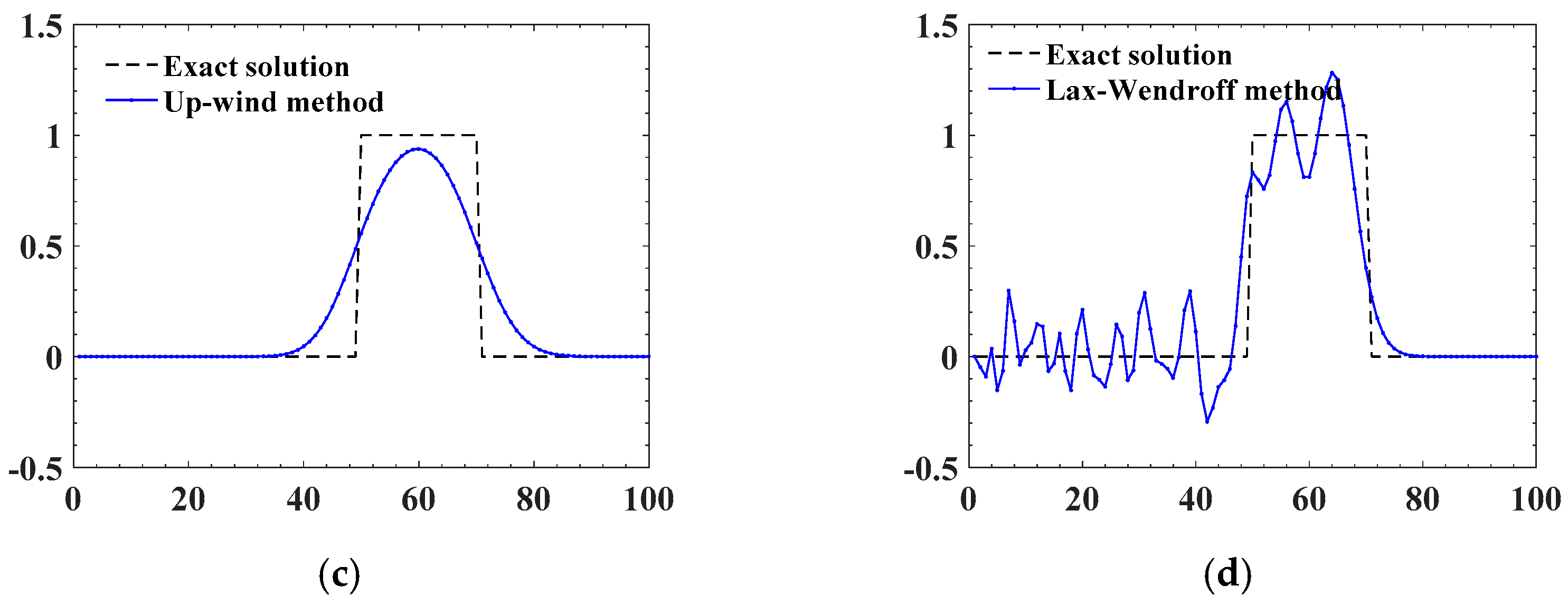
To verify the accuracy and suitablity of the CIP method, a rectangular wave, as shown in Figure 5a, was used to assess the advantages of the CIP method. The control equation is expressed as Equation (16). Moreover, the velocity of propagation is u = 1, the spacial step is Δx = 1, the time step is Δt = 0.1, and the results after 400 steps are shown in Figure 5b–d that includes the CIP method, the up-wind difference method, and the Lax–Wendroff method. Clearly, the CIP method is best suitable for a rectangular wave with large pressure difference. The up-wind method with first-order accuracy is the worst, and the Lax–Wendroff method with second-order accuracy can relativly express the wave-type well, but it has oscillation and divergence in the process. The pressure wave in the pneumatic brake system is large when the brake control valve opens or closes. Thus, it is better to introduce the CIP method for its stability and high accuracy for solving the pressure response with large pressure fluctuation.
3.1.2. Arrangement of the Control Equations
We rearranged Equations (3)–(5) with the CIP method, we rearrange them into advection and non-advection terms. Substituting the gas state equation into Equation (5), the new control equations can be written as
where the left-hand sides hold the advection terms and the right-hand sides hold the non-advection terms. We then rewrite Equations (22)–(24) in vector form as
where
3.1.3. Solving the Control Equations
According to the principle of the CIP method, we differentiate Equation (25) with respect to the spatial variable x, whereupon the derivative form of the equation is obtained as
The CIP method is used to solve hyperbolic PDEs of the form shown in Equation (4). Hence, we should separate the equation into advection and non-advection terms.
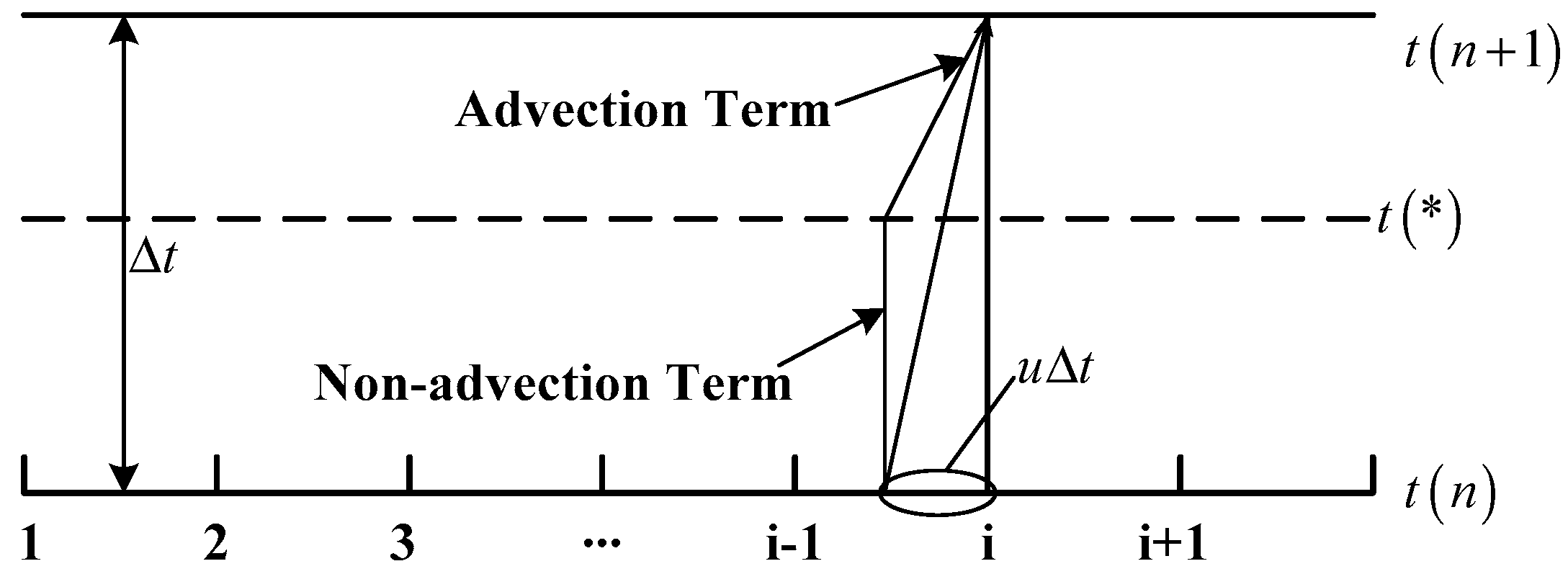
Figure 6 describes the detailed solving principle, in which t(n) indicates a parameter at the current time and t(n + 1) indicates the same parameter but at the next time step. The real process involves a physical quantity being transmitted from t(n) to t(n + 1) in one time step; however, we can deal with it in two steps. The first step is non-advection transmission, which transmits from t(n) to t*; the second step is advection transmission, which transmits from t* to t(n + 1). The value at can be obtained by using Equation (17).
The values of and can be solved directly with an up-wind method as
where
The advection term is
The quantities and are obtained from Equations (29) and (30). Substituting the values into Equations (18)–(21) allows Equations (32) and (33) to be solved using the CIP method.
3.2. Outlet Boundary Settings
According to the principle of the CIP method and Figure 6, the values on the inlet and outlet boundaries cannot be derived but should instead be set directly. Therefore, as shown in Figure 3, we add one more grid at the inlet and outlet separately. Grid zero stands for the air source, and grid N + 1 is the actuator linked to the pipe, which is the brake chamber in this paper. The parameters of grid zero are always the same as those of the air source in the tank, and we focus instead on the settings for grids N and N + 1.
To solve the pressure response in grid N, we deal with it here as a virtual small chamber whose volume is ; the other parameters are shown in Figure 7. The volume is so small that there is no time to exchange heat with the surroundings, so we handle it as an adiabatic chamber. The air flow into the chamber is Gin and the air consumption downstream is Gc, so the pressure response in the chamber can be obtained as
Rewriting Equation (34) in difference form, the pressure is
where
3.3. Discretisation of the Control Equations of the Brake Chamber
To solve the pressure response of the brake chamber simultaneously with that of the pipe, the brake chamber is handled as grid N + 1 and Equations (8), (11) and (13) are rewritten as difference schemes:
where and .
The control equations of the brake circuit were discrete in Section 3.1, Section 3.2 and Section 3.3 , including solving the pipe with the CIP method and the difference scheme used for the brake chamber. Lastly, the solution process is summarized in Figure 8 that is realized by a MATLAB m-file, which leads to obtaining the pressure response in the pipe and brake chamber simultaneously. The main function CIPVec called in Figure 8 can be found in Appendix A.
3.4. The Experiment on the Brake Pressure Response
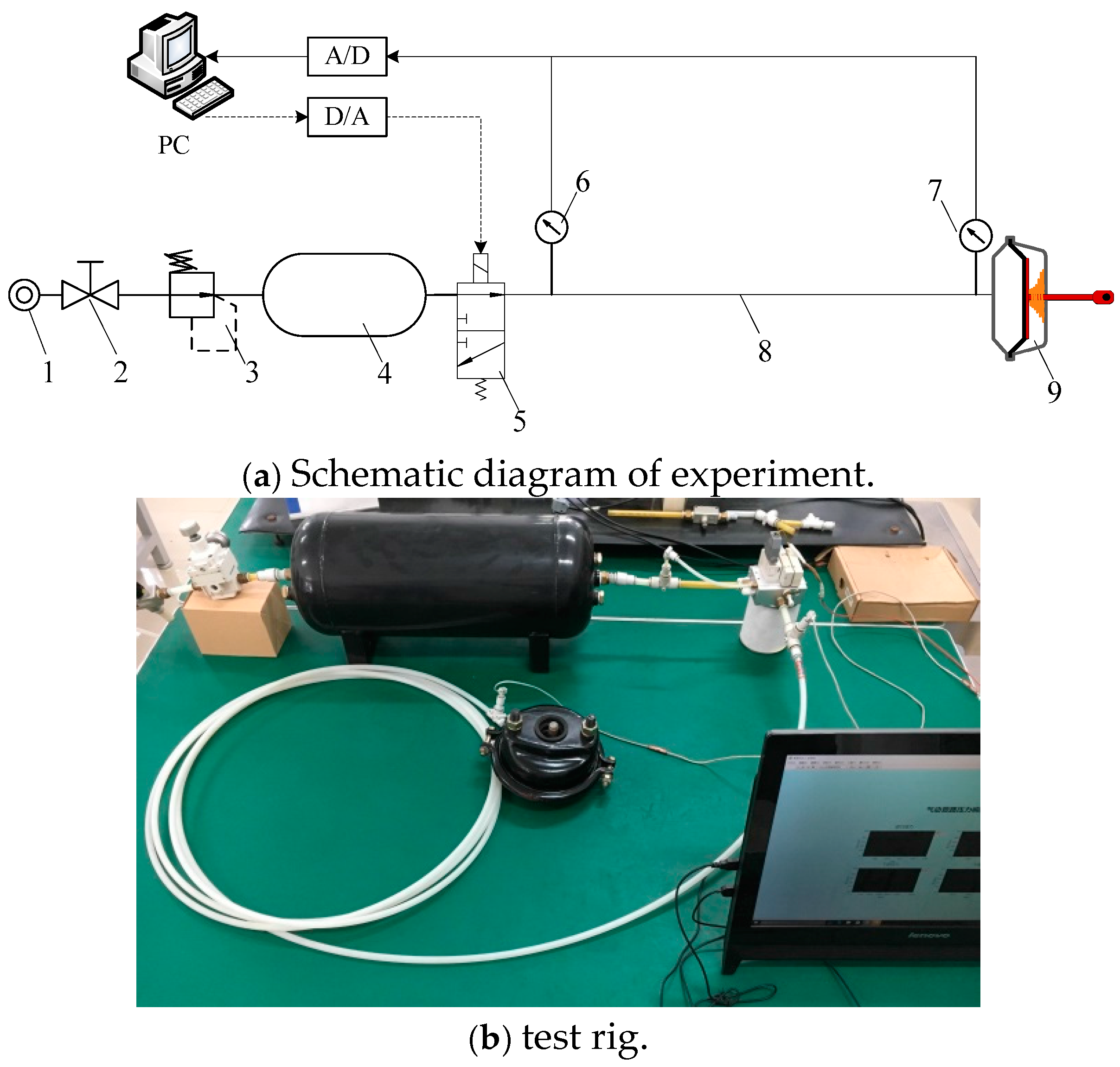
In this experiment, we focused on verifying the mathematical model and the influence of the pipe, so we used a solenoid valve instead of the brake control valve to simplify the measurements. The orifices in Figure 2 are replaced by the solenoid valve and fittings. A brake-circuit test rig was built, as shown in Figure 9. It consists of an air source, a precision regulator (IR3020, SMC), a buffer tank (27 L), a solenoid valve (SY5100, SMC), two pressure sensors (PSE540, SMC), a pipe (T1075, SMC), a brake chamber (C3519VS05D, DONGFENG), and a data acquisition card (NI6009). The accuracy of the pressure sensor is ±0.5% F.S.
4. Results and Discussion
4.1. Experimental Results and Analysis
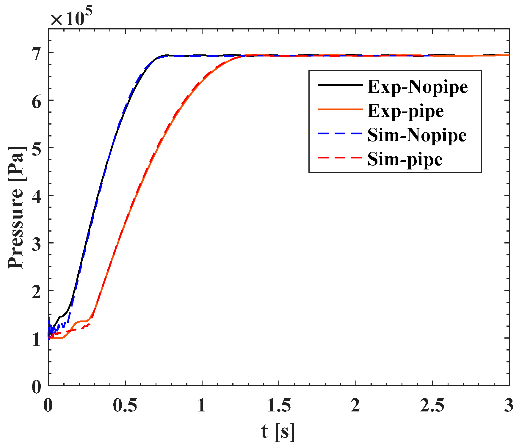
Figure 10 shows the comparison of the experiment and simulation results, and the main parameters settings in simulation are given in Table 2.
Figure 10 indicates that the charge time in the brake chamber is 0.7 s without a pipe and 1.2 s with one. Thus, the time delay is increased by 0.5 s by the pipe restricting the air transmission. For a vehicle being driven at high speed, 0.5 s could cause a serious traffic accident if the brakes cannot be applied promptly. Therefore, the pipe effect must be considered carefully when designing a brake system, and the time delay should be reasonably compensated. In addition, the simulation results are consistent with the experimental ones, which also helps to validate the mathematical models developed in this paper. However, if we look at the results carefully, there is a little deviation at the beginning of the charge. This is because the parameters of the rubber piston are complex and difficult to measure correctly, and the deforming force in the extension process is complex too. Thus, we used an approximate model to describe the piston that causes the deviation.
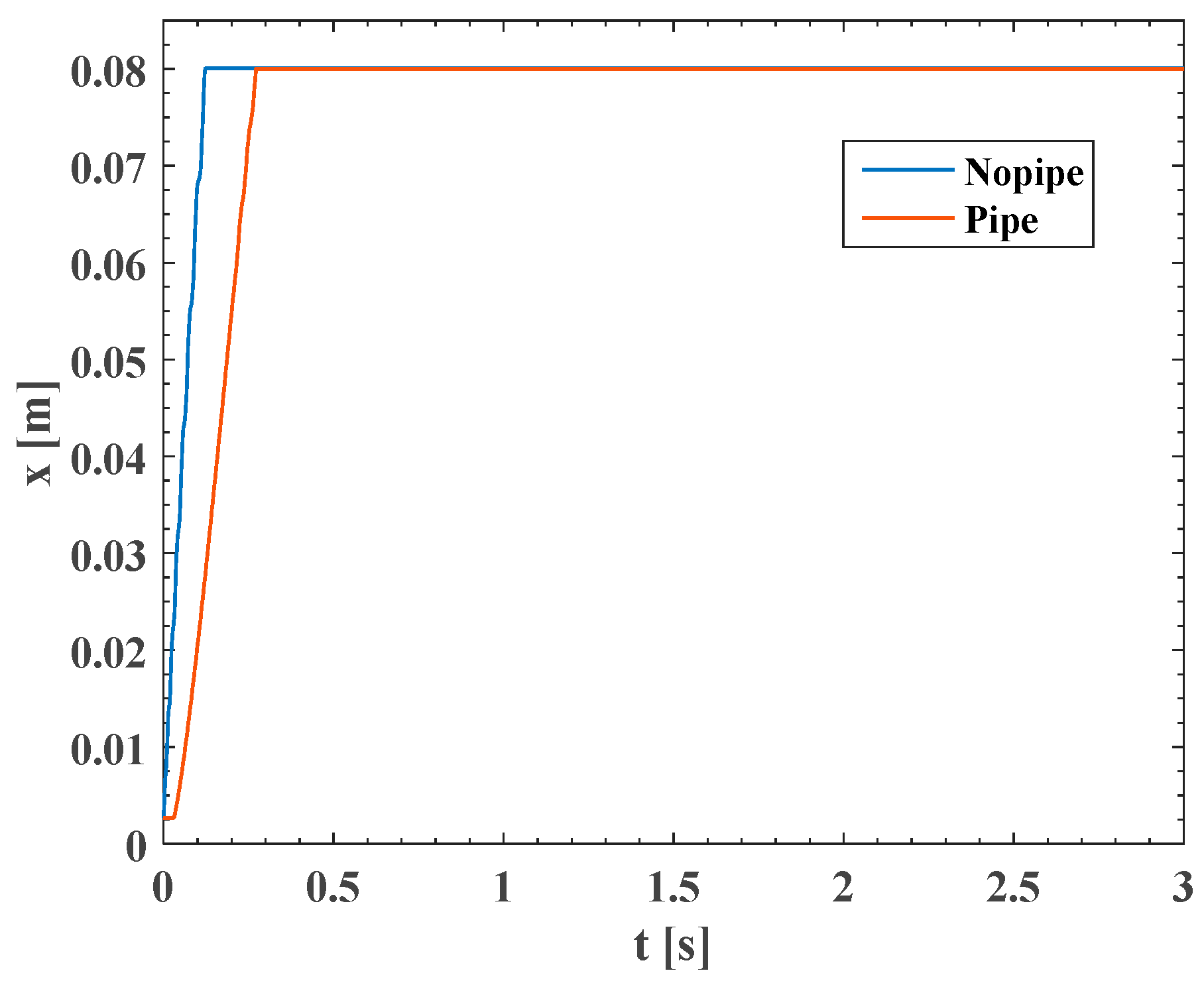
If we combine Figure 10 and Figure 11, it is obvious that the location of the deviation is exactly coincident with the process of the rod extending. Once the rod has extended fully, the rubber deformation has no effect, and the simulation coincides well with the experiment. Furthermore, the pressure in the initial part is very small and it does not begin to brake, so the deviation has little effect on the predicted braking force. Thus, all of this verifies that the CIP method is a precision method for predicting the pressure in the pipe. It also demonstrates that the model and method proposed in this paper are sufficiently accurate to calculate the pressure response of the brake system.
Now that the model has been verified experimentally, we turn our attention to modifying the values of various structural parameters in the simulation to study their effects.
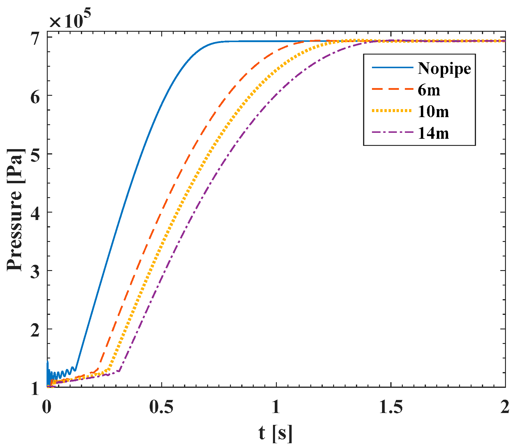
4.2. Influence of Pipe Length
The layout of the brake circuit varies according to the type of vehicle, which in turn could affect the brake pressure response or time delay. Figure 12 shows pressure response curves for different pipe lengths for an inner diameter of 7.5 mm. As the length is increased from 6 m to 14 m, the time delay increases by 0.15 s for every 4 m of pipe. This indicates that the longer the pipe, the more the time delay. Therefore, when we design a brake circuit the pipe should be as short as possible, we should reduce the number of bends, and we should arrange the circuit reasonably, all of which can help to minimise the time delay.
4.3. The Influence of the Pipe Diameter
The most common used pipe diameters for a PBS are in the range 6–16 mm. Figure 13 shows pressure response curves when the diameter is increased from 4 mm to 14 mm. In the simulation, the sonic conductance of the orifice was kept constant to focus on the effect of diameter. As shown, when the diameter varies from 4 to 6 mm, the times delay decreases significantly. However, when the diameter increases from 7.5 to 12 mm, the time delay slightly decreases. However, the time delay increases but does not decrease as the diameter increases from 14 to 16 mm. Clearly, the pipe is similar as a capacitance or resistance according to different pipe length. When the diameter is small, the resistance is with a dominant status compared to capacitance. However, as the diameter increases, the volume increases. Moreover, the condensance gets to be the main influencing factors. Therefore, the time delay decreases first and then increases. However, in actual applications, pipes with a diameter in the range of 4–6 mm are mostly used as control pipes and those in the range of 7.5–12 mm are used as transmission pipes. Therefore, the influence of diameter is relatively small compared to that of length, and so the diameter effect can be neglected. However, for the restriction of the brake control valves, the pipe diameter should be chosen to match the fittings. We can use a smaller diameter if that satisfies the requirements, but we should not use too narrow a pipe with too many transfer joints, because that would increase the local pressure loss.
4.4. Influence of Inlet/Outlet Sonic Conductance
Figure 13 indicates that the influence of the pipe diameter is minimal. However, for the pipe restriction, the diameter of the fittings is limited, so we should consider the influence of the inlet or outlet sonic conductance. Figure 14 shows pressure response curves for different orifice sizes. Here, O1 is orifice 1 in Figure 2 and O2 is orifice 2. By comparing curves 1 and 2, we see that the time delay increases significantly as the orifice shrinks. If we compare curves 3 and 4, we see that the pressure response depends on the orifice arrangement: when the larger orifice is in the front, the pressure response is quicker. The main reason for this phenomenon is that the orifice size restricts the flow rate; there will be a large pressure drop if the section area changes abruptly, whereupon the flow rate and charging speed will decrease simultaneously. Thus, when we design a brake circuit, the arrangement of the components should reduce gradually to decrease the local pressure drop.
4.5. Influence of the Thermodynamic Model
In the former, we have identified the influence of the pipe when the brake chamber is charged. However, if the brake chamber is modelled using different thermodynamic assumptions, the pressure response is different. The most-used model is either the adiabatic model or the isothermal model. To understand the influence of the thermodynamic model, we compare different ones here. As shown in Figure 15, when heat exchange is taken into consideration, the model is more like the adiabatic one. Figure 15 also shows the temperature change to be as high as 70 K, in which case the isothermal model produces large deviations and cannot reflect the real pressure response in the brake chamber.
4.6. Comphensive Analysis of Structure Parameters
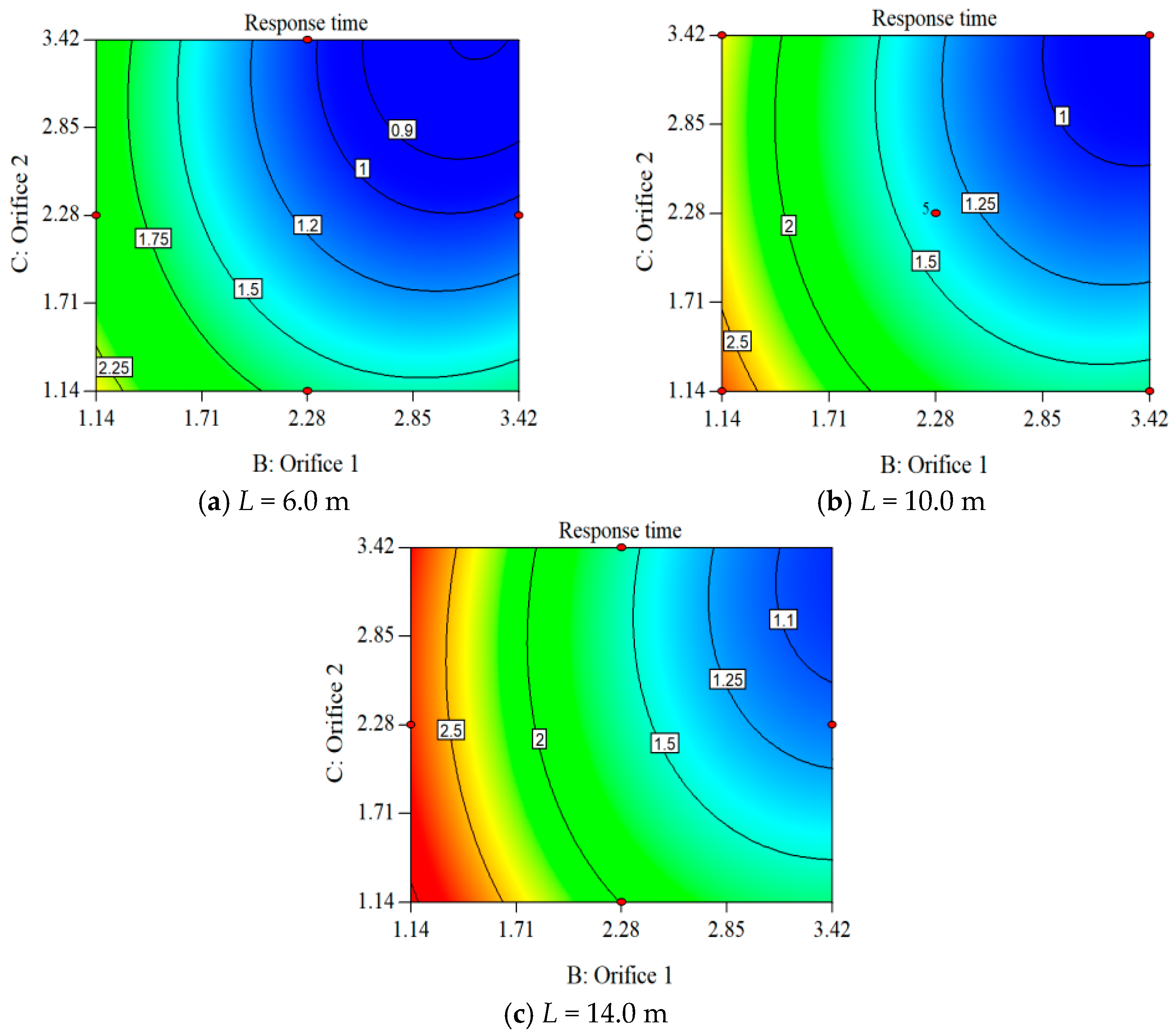
As shown in Figure 12, the pressure response time gets larger when the pipe length increases. However, here we focus more on the relationship between time delay and pipe length. In other words, we want to find out time delay that occurs due to different parameter configurations. Though the range of actuation pressure and pipe length is limited, the combination forms of these structure parameters are various. Then, we introduced the response surface method [34] to predict the regularity between different simulation conditions. Here a simulation experiment with three factors (Length, CO1, and CO2) and three levels (as shown in Table 3) was designed by Design-Expert [35]. In these experiment groups, the diameter was constant at 7.5 mm, and the heat exchange model was used. The experiment was run 17 times, as shown in Table 3, and the response times were obtained, as shown in Figure 16.
Figure 16 shows that the response time by contour and the white labels in the graph are the response times. Clearly, the response time varies significantly when the configuration changes. For example, when the pipe length is 10 m, the response time varies from 0.94 s to 2.66 s. It is also seen that increasing the sonic conductance of an orifice decreases the response time. However, if the orifice 1 is constant and relatively smaller, the response time will vary slightly by increasing the orifice 2. This graph also presents a reference for design and analysis.
5. Conclusions
In this study, a pressure response model of a brake circuit was developed by considering the influence of the pipe. The pipe model took into consideration heat transfer and unsteady friction, and was solved by introducing the CIP method with its third-order accuracy. Meanwhile, the brake-chamber model considered heat transfer, thereby further improving the accuracy. Lastly, the model was verified experimentally and was shown to be highly accurate and suitable. The conclusions drawn from this study can be summarised as follows:
- (1)
- Because there is a time delay associated with air flow in the pipe, the brake pressure response obviously lags. In this study, the time delay varies from 0.9 s to 2.85 s with a different parameters configuration; therefore, the time delay should be carefully considered when designing the brake circuit.
- (2)
- The brake pressure response time increased significantly with pipe length, but the diameter of a pipe has less effect when the diameter is in the range of 7.5–12 mm. Moreover, the effect of pipe volume gets larger compared with resistance when the diameter further increases.
- (3)
- The inlet and outlet sonic conductances affected the pressure response to different degrees. The time delay increases when the sonic conductance decreases, and they should be matched carefully.
- (4)
- The brake-chamber model was the most accurate when considering the heat transfer. Compared with the isothermal model, the adiabatic model was more accurate for temperature changes up to 70 K.
- (5)
- The CIP method could be used to calculate the pressure response in the pipe and was verified to be highly accurate and stable.
Here, we proposed the method and algorithm to solve the pressure response time of a pneumatic brake circuit. It is useful to simplify the process of designing brake systems. In the future, we intend to further develop this method and make the algorithms programmed. This will make it better suited to engineering applications, and it will also possess high efficiency and accuracy.
Acknowledgments
The authors acknowledge the SMC Corporation for the financial support and technical advice.
Author Contributions
Gangyan Li and Toshiharu Kagawa conceived this study and proposed the analysis method; Fan Yang designed the experiment; Jian Hua and Xingli Li performed the experiments and analyzed the data; Fan Yang wrote the paper and Gangyan Li modified the final paper.
Conflicts of Interest
The authors declare no conflict of interest.
Nomenclature
| A | area of piston [m2] |
| b | critical pressure ratio |
| cv | specific heat at constant volume [J/(kg·K)] |
| cp | specific heat at constant pressure [J/(kg·K)] |
| C | sonic conductance [m3/(s·Pa)] |
| d | diameter of brake chamber [m] |
| D | inner diameter of pipe [m] |
| e | inner energy [J] |
| Fd | deforming force [N] |
| G | mass flow rate [kg/s] |
| h | coefficient of heat convection [W/(m2·K)] |
| H | enthalpy [J] |
| k | spring constant [N/m] |
| L | length of pipe [m] |
| M | mass of piston [kg] |
| p | pressure [Pa] |
| R | gas state constant = 287 [J/(kg·K)] |
| s | stroke of push rod [m] |
| Sh | heat exchange area [m2] |
| t | time [s] |
| u | velocity [m/s] |
| Vc | volume [m3] |
| x | displacement [m] |
| κ | specific heat index = 1.4 |
| θ | temperature [K] |
| ρ | density [kg/m3] |
| Subscripts | |
| 0 | stand reference state (20 °C, 100 kPa) |
| 1 | upstream |
| 2 | downstream |
| c | brake chamber |
Appendix A
The main function of CIPVec called in Figure 8 is given as follows:
| function [FN,GN] = CIPVec(NX,YU,DT,DX,F,G) |
| % NX-the numbers of grids |
| % YU-the velocity of advection |
| % DT-the length of time step |
| % DX-the length of spatial step |
| % F/G-the parameters under solving and its differential |
| % FN/GN-the values of F/G in next time step |
| for i = 2:NX − 1 |
| if YU(i) < 0 |
| ISG = 1; |
| else |
| ISG = −1; |
| end |
| IUP = i + ISG; |
| XX = -YU(i)*DT; |
| FDIF = (F(IUP) − F(i))/DX*ISG; |
| XAM1 = (G(i) + G(IUP) − 2.0*FDIF)/(DX*DX); |
| XBM1 = (3.0*FDIF − 2*G(i) − G(IUP))/DX*ISG; |
| FN(i) = ((XAM1*XX + XBM1)*XX + G(i))*XX + F(i); |
| GN(i) = (3.0*XAM1*XX + 2.0*XBM1)*XX + G(i); |
| end |
References
- Fujino, K.; Taniguchi, K.; Yamamoto, N.; Youn, C.; Kagawa, T. Transient pressure and flow rate measurement of pneumatic power supply line in Shinkansen: Examination of unsteady characteristics in pneumatic supply system by experiment. In Proceedings of the 2010 SICE Annual Conference, Taipei, Taiwan, 18–21 August 2010; pp. 1664–1669. [Google Scholar]
- Selvaraj, M.; Gaikwad, S.; Suresh, A.K. Modeling and Simulation of Dynamic Behavior of Pneumatic Brake System at Vehicle Level. SAE Int. J. Commer. Veh. 2014, 11, 1–9. [Google Scholar] [CrossRef]
- Lopez, A.; Sherony, R.; Chien, S.; Li, L.; Qiang, Y.; Chen, Y. Analysis of the braking behaviour in pedestrian automatic emergency braking. In Proceedings of the 2015 IEEE 18th International Conference on Intelligent Transportation Systems (ITSC), Las Palmas, Spain, 15–18 September 2015; pp. 1117–1122. [Google Scholar]
- Karthikeyan, P.; Chaitanya, C.S.; Raju, N.J.; Subramanian, S.C. Modelling an electropneumatic brake system for commercial vehicles. IET Electr. Syst. Transp. 2011, 1, 41–48. [Google Scholar] [CrossRef]
- Fleming, B. Advances in automotive electronics [automotive electronics]. IEEE Veh. Technol. Mag. 2015, 10, 4–11. [Google Scholar] [CrossRef]
- Wang, Z.; Zhou, X.; Yang, C.; Chen, Z.; Wu, X. An Experimental Study on Hysteresis Characteristics of a Pneumatic Braking System for a Multi-Axle Heavy Vehicle in Emergency Braking Situations. Appl. Sci. 2017, 7, 799. [Google Scholar] [CrossRef]
- Qin, T. Research on Delay Time Analysis and Its Control Techniques of Bus Pneumatic Brake System. Ph.D. Thesis, Wuhan University of Technology, Wuhan, China, 2012. [Google Scholar]
- Long, X.; Hu, X. Optimization on the response time of pneumatic brake systems of commercial vehicle. Enterp. Sci. Technol. Dev. 2013, 365, 44–46. (In Chinese) [Google Scholar]
- Mithun, S.; Gayakwad, S. Modeling and simulation of pneumatic brake system used in heavy commercial vehicle. IOSR J. Mech. Civ. Eng. 2014, 11, 1–9. [Google Scholar] [CrossRef]
- Modeling and Simulation Vehicle Air Brake System. Available online: https://www.modelica.org/events/modelica2011/Proceedings/pages/papers/17_3_ID_144_a_fv.pdf (accessed on 13 September 2017).
- Li, S.; Bao, W. Analysis of transient hydraulic pressure pulsation in pipelines using MATLAB Simulink. Eng. Mech. 2006, 23, 184–188. [Google Scholar]
- Tokashiki, L.; Fujita, T.; Kagawa, T. Simulation on pneumatic cylinder including pipes. Hydraul. Pneum. 1997, 28, 766–771. (In Japanese) [Google Scholar] [CrossRef]
- Zielke, W. Frequency Dependent Friction in Transient Pipe Flow; University of Michigan: Ann Arbor, MI, USA, 1966. [Google Scholar]
- Kitagawa, A.; Kagawa, T.; Takenaka, T. High speed and accurate computing method for transient response of pneumatic transmission line using characteristics method. Trans. Soc. Instrum. Control Eng. 1984, 20, 648–653. [Google Scholar] [CrossRef]
- Hashimoto, K.; Imaeda, M.; Kikuchi, K. The analyses of transient responses of fluid lines by characteristics grid method. Hydraul. Pneum. 1985, 16, 140–146. (In Japanese) [Google Scholar] [CrossRef]
- Wei, W.; Du, N. Influence of braking pipe on braking performance for heavy haul train. J. Traffic Transp. Eng. 2011, 5, 49–54. [Google Scholar]
- Wei, W.; Wu, X. Influence of Brake Characteristics on Longitudinal Impulse of Train. J. Dalian Jiaotong Univ. 2012, 2, 1–5. [Google Scholar]
- Yabe, T.; Aoki, T.; Sakaguchi, G.; Wang, P.Y.; Ishikawa, T. The compact CIP (Cubic-Interpolated Pseudo-particle) method as a general hyperbolic solver. Comput. Fluids 1991, 19, 421–431. [Google Scholar] [CrossRef]
- Takewaki, H.; Nishiguchi, A.; Yabe, T. Cubic interpolated pseudo-particle method (CIP) for solving hyperbolic-type equations. J. Comput. Phys. 1985, 61, 261–268. [Google Scholar] [CrossRef]
- Zhao, X.; Liu, B.; Liang, X. Constrained interpolation profile (CIP) method and its application. J. Ship Mech. 2016, 20, 393–402. [Google Scholar]
- Zhao, X.; Fu, Y.; Zhang, D. Numerical simulation of flow past a cylinder using a CIP-based model. J. Harbin Eng. Univ. 2016, 37, 297–305. [Google Scholar]
- Pang, P.T.; Agnew, D. Brake System Component Characterization for System Response Performance: A System Level Test Method and Associated Theoretical Correlation; SAE Technical Paper; SAE International: Detroit, MI, USA, 2004. [Google Scholar]
- Yang, F.; Li, G.; Hu, J.; Liu, W.; Qi, W. Method for resultant and calculating the flow-rate characteristics of pneumatic circuit. In Proceedings of the 2015 International Conference on Fluid Power and Mechatronics (FPM), Harbin, China, 5–7 August 2015; pp. 379–384. [Google Scholar]
- Pneumatic Fluid Power—Determination of Flow-Rate Characteristic of Component Using Compressible Fluids—Part 1: General Rules and Test Methods for Steady-State Flow; ISO 6358-1; International Organization for Standardization (ISO): Geneva, Switzerland, 2013.
- Pneumatic Fluid Power—Assessment of Component Reliability by Testing—Part 2: Directional Control Valves; ISO 19973-2; International Organization for Standardization (ISO): Geneva, Switzerland, 2015.
- Wang, T.; Peng, G.; Toshiharu, K. Measurement and Resultant Methods of Flow-rate Characteristics of Small Pneumatic Valves. J. Mech. Eng. 2009, 45, 290–297. (In Chinese) [Google Scholar] [CrossRef]
- Niu, J.L.; Shi, Y.; Cao, Z.X.; Cai, M.L.; Chen, W.; Zhu, J.; Xu, W.Q. Study on air flow dynamic characteristic of mechanical ventilation of a lung simulator. Sci. China Technol. Sci. 2017, 60, 243–250. [Google Scholar] [CrossRef]
- Shi, Y.; Jia, G.W.; Cai, M.; Xu, W.Q. Study on the dynamics of local pressure boosting pneumatic system. Math. Probl. Eng. 2015, 2015, 849047. [Google Scholar] [CrossRef]
- Kaasa, G.-O.; Chapple, P.J.; Lie, B. Modeling of an electro-pneumatic cylinder actuator for nonlinear and adaptive control, with application to clutch actuation in heavy-duty trucks. In Proceedings of the 3rd FPNI PhD International Symposium on Fluid Power, Terrassa, Spain, 30 June–2 July 2004. [Google Scholar]
- Matsuo, K. Compressible Fluid Flow—Theory and Analysis of Internal Flow; Rikogakusha Publishing: Tokyo, Japan, 1999; pp. 145–147. [Google Scholar]
- Shiraishi, K.; Matsuoka, T. The simulation of acoustic wave propagation by using characteristic curves with CIP method. Butsuri Tansa 2006, 59, 261–274. (In Japanese) [Google Scholar] [CrossRef]
- Guo, Z.; Li, X.; Kagawa, T. Heat transfer effects on dynamic pressure response of pneumatic vacuum circuit. In Proceedings of the ASME/JSME 2011 8th Thermal Engineering Joint Conference, Honolulu, HI, USA, 13–17 March 2011. [Google Scholar]
- Qi, W.; Li, G.; Lu, Q.; Long, X. Influence of Bus Brake Chamber Inlet Diameter on Pressure Characteristic. Hydraul. Pneum. Seals 2016, 36, 21–25. (In Chinese) [Google Scholar]
- Nouby, M.; Mathivanan, D.; Srinivasan, K. A combined approach of complex eigenvalue analysis and design of experiments (DOE) to study disc brake squeal. Int. J. Eng. Sci. Technol. 2009, 1, 254–271. [Google Scholar] [CrossRef]
- Li, L.; Sai, Z.; Qiang, H. Application of response surface methodology in experiment design and optimization. Res. Explor. Lab. 2015, 34, 41–45. (In Chinese) [Google Scholar]
Figure 1.
Schematic of the pneumatic brake circuit of a bus.
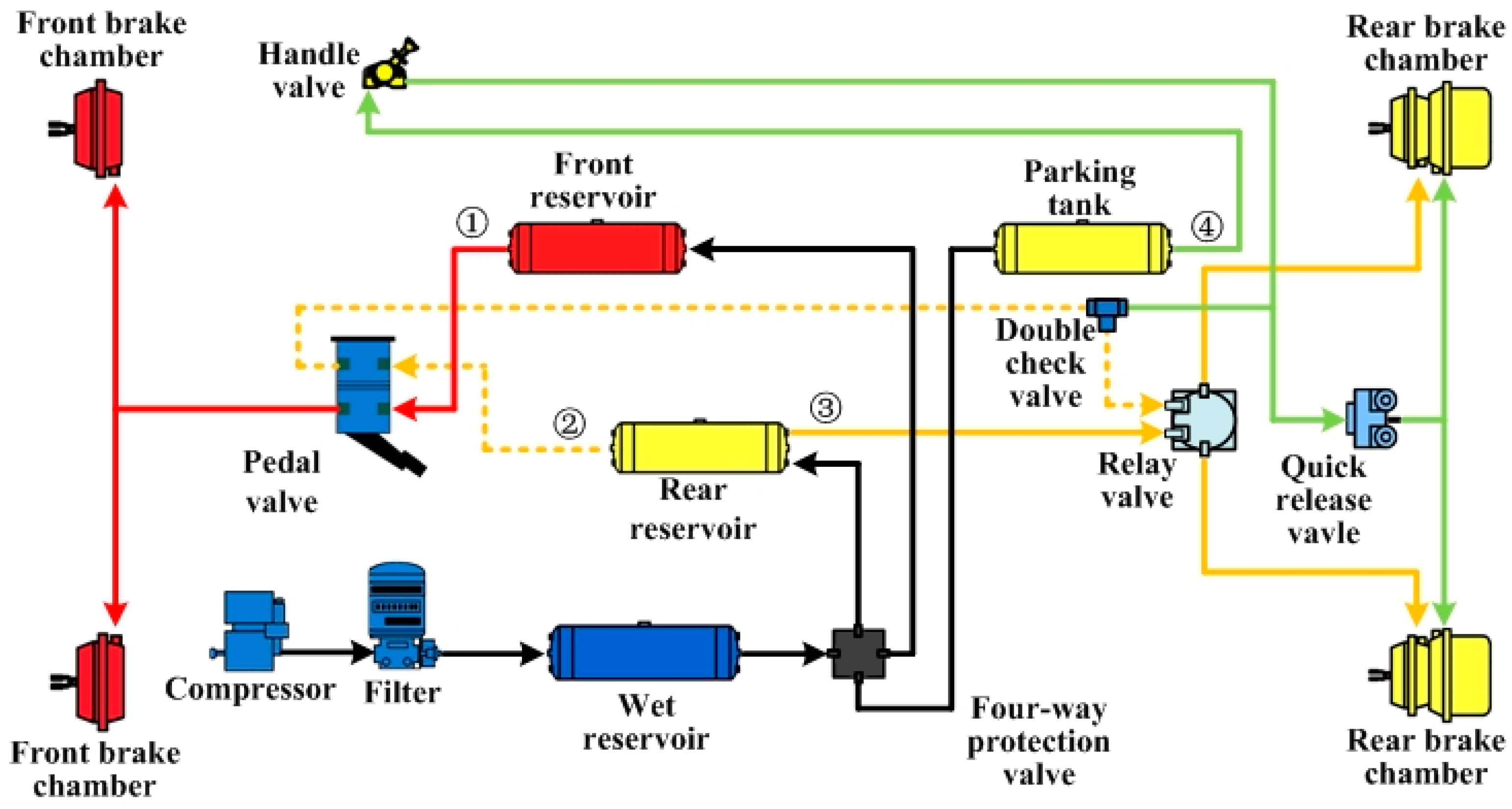
Figure 2.
Simplified pneumatic brake circuit.

Figure 3.
Analysis model of pipe.

Figure 4.
Structural diagram of brake chamber.

Figure 5.
Comparison of different difference schemes. (a) Initial value; (b) CIP method; (c) Up-wind method; (d) Lax–Wendroff method
Figure 5.
Comparison of different difference schemes. (a) Initial value; (b) CIP method; (c) Up-wind method; (d) Lax–Wendroff method


Figure 6.
Principle of CIP method.

Figure 7.
Model of the outlet boundary.
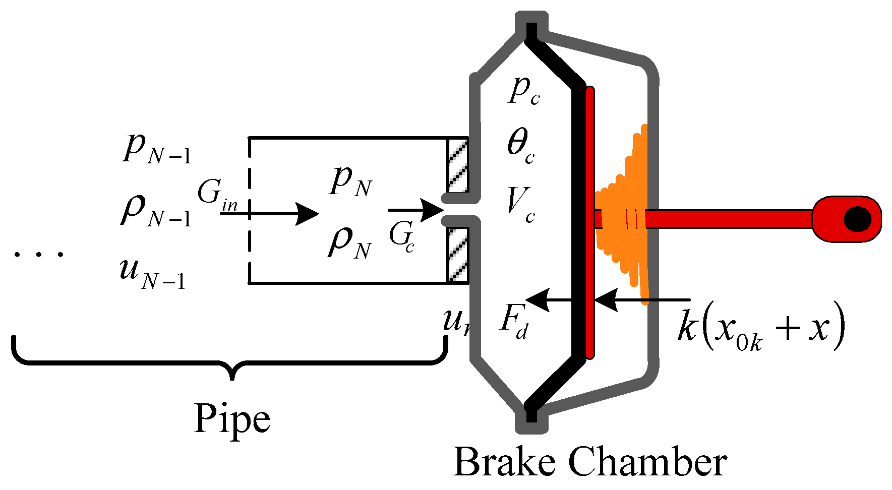
Figure 8.
Flow-chart of brake circuit simulation.
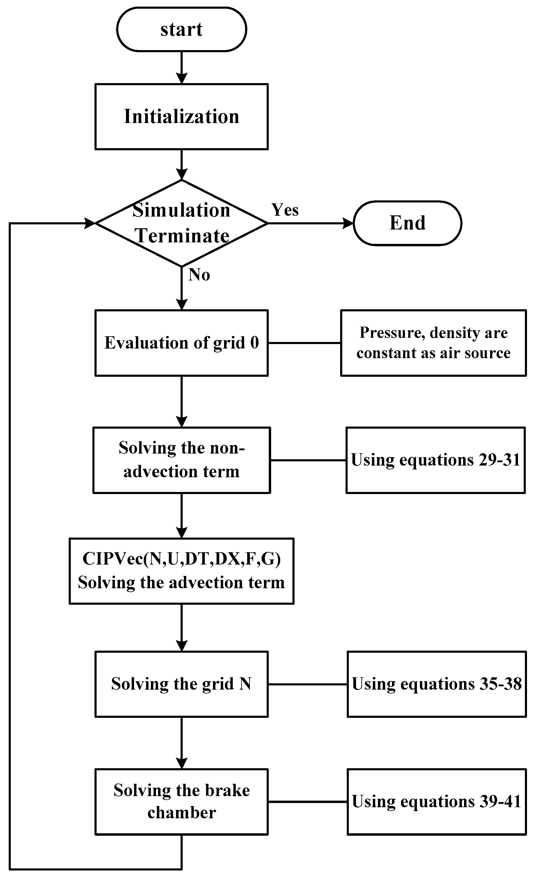
Figure 9.
Schematic diagram of pneumatic brake circuit. (a) Schematic diagram of experiment. 1—Air source; 2—shut-off valve; 3—precision regulator; 4—buffer tank; 5—solenoid valve; 6,7—pressure sensor; 8—pipe; 9-brake—chamber; and (b) test rig.
Figure 9.
Schematic diagram of pneumatic brake circuit. (a) Schematic diagram of experiment. 1—Air source; 2—shut-off valve; 3—precision regulator; 4—buffer tank; 5—solenoid valve; 6,7—pressure sensor; 8—pipe; 9-brake—chamber; and (b) test rig.

Figure 10.
Pressure response curves in brake chamber.

Figure 11.
Displacement curves of piston in brake chamber.

Figure 12.
Pressure curves for different pipe lengths.

Figure 13.
Pressure curves for different pipe diameters.
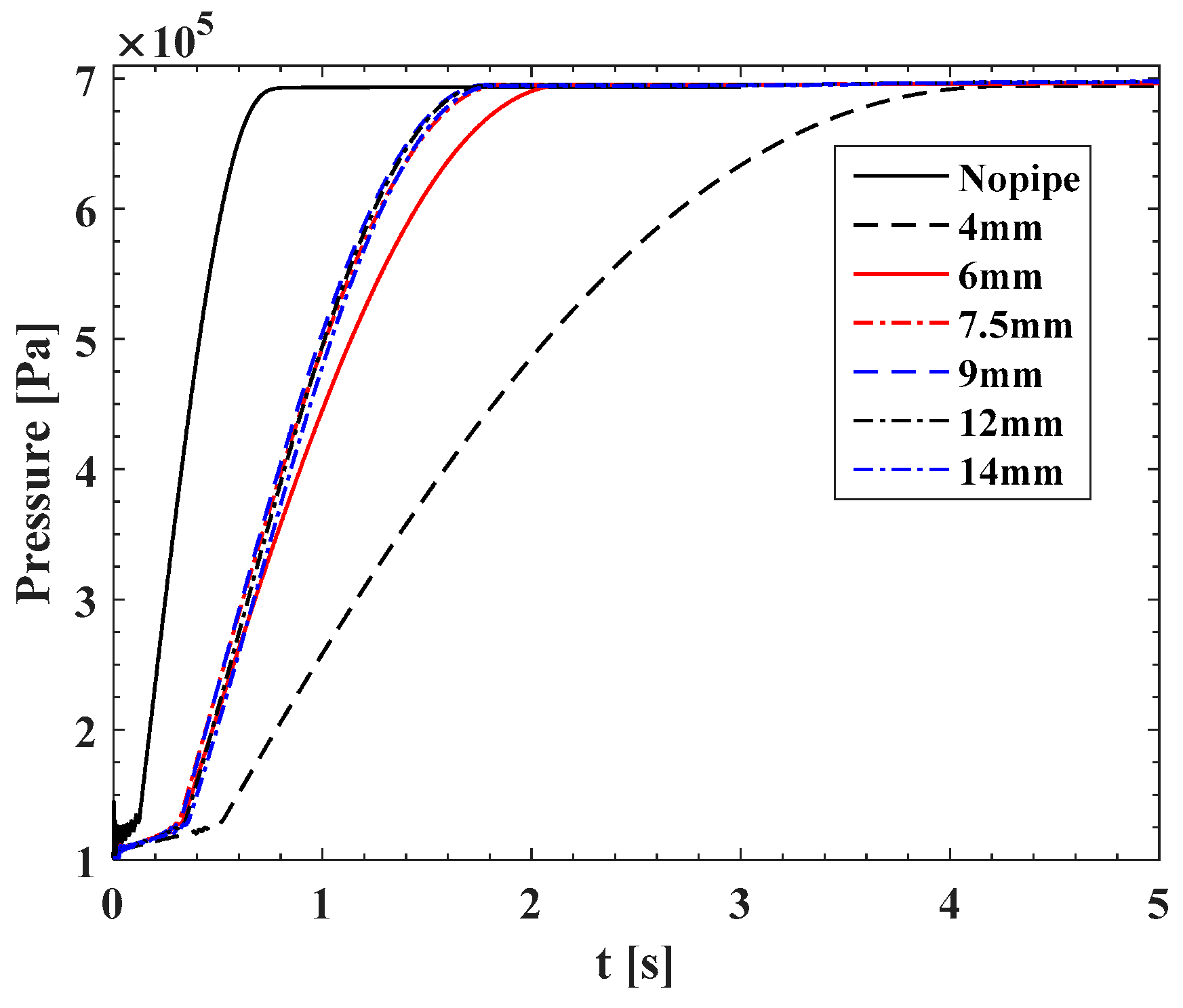
Figure 14.
Pressure curves for different sonic conductances.
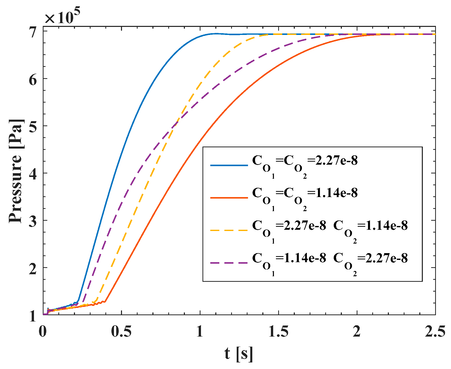
Figure 15.
Pressure and temperature curves for different thermodynamics models.
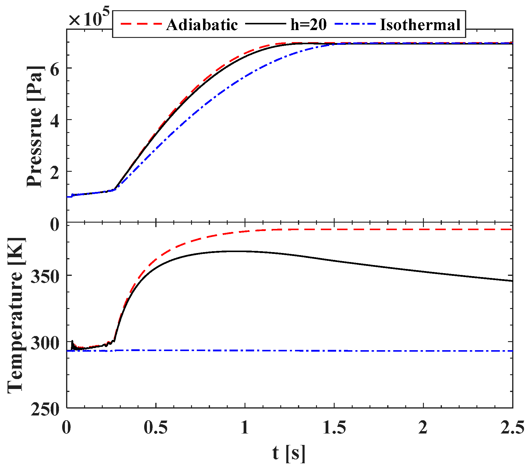
Figure 16.
Pressure response time for different parameters configuration.


Table 1.
Influence degree of time delay on braking distance.
| Time Delay (s) | Increasing of Brake Distance (m) | Influence Degree (%) | Remarks |
|---|---|---|---|
| 0.9 | 15.0 | 40.9 | The whole brake distance is assumed to satisfy the force law, and it is equal to 36.7 m |
| 0.7 | 11.7 | 31.8 | |
| 0.5 | 8.3 | 22.7 | |
| 0.3 | 5.0 | 13.6 |
Table 2.
Simulation parameters of brake pressure response.
| Components | Brake Chamber | Pipe | Solenoid Valve | |||||
|---|---|---|---|---|---|---|---|---|
| Parameters | s [mm] | k [N/m] | x0 [mm] | d [cm] | L [m] | D [mm] | C [m3/(s·Pa)] | b |
| Values | 80 | 3000 | 2.7 | 16 | 10 | 7.5 | 2.27 × 10⁻⁸ | 0.38 |
Table 3.
Arrangement of the simulation experiment.
| No. | Length [m] | CO1 [×10−8 m3/(s·Pa)] | CO2 [×10−8 m3/(s·Pa)] | Response Time [s] |
|---|---|---|---|---|
| 1 | 14.0 | 2.28 | 1.14 | 1.95 |
| 2 | 10.0 | 3.42 | 1.14 | 1.65 |
| 3 | 14.0 | 1.14 | 2.28 | 2.85 |
| 4 | 14.0 | 2.28 | 3.42 | 1.52 |
| 5 | 14.0 | 3.42 | 2.28 | 1.18 |
| 6 | 10.0 | 2.28 | 2.28 | 1.36 |
| 7 | 10.0 | 1.14 | 1.14 | 2.66 |
| 8 | 6.0 | 1.14 | 2.28 | 1.98 |
| 9 | 10.0 | 2.28 | 2.28 | 1.37 |
| 10 | 10.0 | 2.28 | 2.28 | 1.37 |
| 11 | 6.0 | 2.28 | 3.42 | 1.07 |
| 12 | 6.0 | 3.42 | 2.28 | 0.96 |
| 13 | 10.0 | 3.42 | 3.42 | 0.94 |
| 14 | 10.0 | 2.28 | 2.28 | 1.37 |
| 15 | 10.0 | 1.14 | 3.42 | 2.35 |
| 16 | 6.0 | 2.28 | 1.14 | 1.71 |
| 17 | 10.0 | 2.28 | 2.28 | 1.37 |
© 2017 by the authors. Licensee MDPI, Basel, Switzerland. This article is an open access article distributed under the terms and conditions of the Creative Commons Attribution (CC BY) license (http://creativecommons.org/licenses/by/4.0/).
Share and Cite
MDPI and ACS Style
Yang, F.; Li, G.; Hua, J.; Li, X.; Kagawa, T. A New Method for Analysing the Pressure Response Delay in a Pneumatic Brake System Caused by the Influence of Transmission Pipes. Appl. Sci. 2017, 7, 941. https://doi.org/10.3390/app7090941
AMA Style
Yang F, Li G, Hua J, Li X, Kagawa T. A New Method for Analysing the Pressure Response Delay in a Pneumatic Brake System Caused by the Influence of Transmission Pipes. Applied Sciences. 2017; 7(9):941. https://doi.org/10.3390/app7090941
Chicago/Turabian StyleYang, Fan, Gangyan Li, Jian Hua, Xingli Li, and Toshiharu Kagawa. 2017. "A New Method for Analysing the Pressure Response Delay in a Pneumatic Brake System Caused by the Influence of Transmission Pipes" Applied Sciences 7, no. 9: 941. https://doi.org/10.3390/app7090941
Note that from the first issue of 2016, this journal uses article numbers instead of page numbers. See further details here.