Practical Challenge of Shredded Documents: Clustering of Chinese Homologous Pieces

1
School of Physics and Optoelectronic Engineering, Xidian University, Xi’an 710071, China
2
School of Automation and Information Engineering, Xi’an University of Technology, Xi’an 710048, China
*
Author to whom correspondence should be addressed.
Appl. Sci. 2017, 7(9), 951; https://doi.org/10.3390/app7090951
Submission received: 20 July 2017
/
Revised: 7 September 2017
/
Accepted: 12 September 2017
/
Published: 15 September 2017
Abstract
:When recovering a shredded document that has numerous mixed pieces, the difficulty of the recovery process can be reduced by clustering, which is a method of grouping pieces that originally belonged to the same page. Restoring homologous shredded documents (pieces from different pages of the same file) is a frequent problem, and because these pieces have nearly indistinguishable visual characteristics, grouping them is extremely difficult. Clustering research has important practical significance for document recovery because homologous pieces are ubiquitous. Because of the wide usage of Chinese and the huge demand for Chinese shredded document recovery, our research focuses on Chinese homologous pieces. In this paper, we propose a method of completely clustering Chinese homologous pieces in which the distribution features of the characters in the pieces and the document layout are used to correlate adjacent pieces and cluster them in different areas of a document. The experimental results show that the proposed method has a good clustering effect on real pieces. For the dataset containing 10 page documents (a total of 462 pieces), its average accuracy is 97.19%.
1. Introduction
Shredded document recovery is a complicated and challenging problem that has been studied by many researchers. Paper documents are separated into large numbers of pieces when they are shredded. These pieces are highly similar and present chaotic sequences, thereby increasing the difficulty of document recovery. Shredded document recovery has important research value, and the relevant findings can be extensively applied in several fields, such as information security [1], judicial investigations [2], and archaeological research [3].
Shredded document recovery is a complicated non-deterministic polynomial-hard problem [4]. The recovery task includes several steps, and piece clustering is one of the key steps [5]. As the number of pieces increases, the difficulty of document recovery also increases [6]. In clustering, a large number of pieces are grouped into several clusters, and the pieces in the cluster are processed together, thereby reducing the difficulty of piece searching and improving the accuracy of piece matching [7]. Because of the high similarity between shreds, piece clustering is difficult.
Research on piece clustering can be divided into two categories.
The first piece clustering category is based on a single-page document. Wang et al. [8] considered piece clustering according to the distribution feature of a text line and assessed cluster validity by the matching proportion method. Sleit et al. [9] treated the clustering operation as a part of document reconstruction itself and used the cost function for piece matching and clustering. Richter et al. [10] utilized multimodal features, including shape, context, etc., to combine clusters and assemble shredded documents. Lei [11] used line information to cluster pieces from the same line. Similarly, Guo et al. [12] presented a row clustering method for shreds.
The second piece clustering category is based on multi-page documents. Ukovich et al. [5] employed a 12-dimension feature that included line spacing and paper/ink color. Based on the features, virtually shredded pieces from different files are clustered using hierarchical clustering. Schoier [13] used only the text line position as the feature to cluster pieces from multi-page documents, which have distinctly different page setups. Diem et al. [14] used several methods (color analysis, paper type analysis, and classification of the text) to cluster pieces from different sources. Chanda et al. [15] employed clustering as a preprocessing step for piece forensics and analyzed paper color and background texture to achieve piece clustering from different files. Liu et al. [16] proposed a spectral clustering algorithm that is based on the contour and color distribution of pieces, and several photos shredded by hand were clustered. Lalitha et al. [17] applied the shape information of pieces as the matching feature, clustered the different pages shredded by hand and reassembled the pieces.
Differing from the first study that focused on a few of pieces and used the clustering idea to achieve pieces matching and splicing. The second study must solve the problem of piece clustering, in which numerous pieces from different documents are mixed. Because of its highly applicable value, the second study is a hotspot in the current research of piece clustering. Although some achievements have been made in the second study, it focuses on the pieces that have distinct differences regarding page format (character size and lines spacing), appearance (paper color and piece shape), or content (writing style). These visual differences are very helpful for clustering. However, a real file usually has a unified document format, in which all pages of the document must present consistent paper color, character size, and text line spacing to satisfy people's reading habits [18]. When the file is shredded, the produced pieces are highly similar regarding page format, appearance, and content. Because these pieces are derived from the same file, we refer to them as homologous pieces, as shown in Figure 1. Unlike the study objects in existing research, this paper addresses homologous pieces with a similar appearance. Distinguishing the pieces from different pages is difficult. Minimal differences among homologous pieces are observed, which hinders clustering using the features proposed in previous studies. Due to the ubiquitous nature of homologous pieces (they are extensively distributed in shredded documents), research on homologous piece clustering is significant to real shredded document recovery. Because China is an influential country and the use of Chinese is extensive, millions of Chinese documents are produced every year; thus, Chinese shredded document recovery is in huge demand. Therefore, this paper focuses on the problem of Chinese homologous piece clustering.
The contributions of this paper are as follows.
- In contrast to existing studies, this paper addresses homologous pieces that have unified page format and high similarity with regard to content and appearance. As a result, clustering is very difficult. Since homologous pieces are prevalent in shredded documents and there is a high demand for recovery of these pieces, the study of this paper has important practical significance.
- Because a document page includes only one leftmost piece and one rightmost piece, this paper can calculate the number of pages by recognizing the leftmost and rightmost pieces, thereby establishing a basis for obtaining the optimal clustering number.
- By determining the correlations between characters and between characters and blank spaces in adjacent text lines, this paper matches the leftmost piece with the rightmost piece from the same page, thereby providing a good starting point for piece clustering.
- Proceeding from the document, which is the source of the pieces, we propose a method of piece clustering that is based on the document layout. This method distinguishes pieces by the area in the document to which they belonged and uses the correlations between shreds to achieve effective clustering.
2. Clustering Method for Chinese Homologous Pieces
The clustering of Chinese homologous pieces involves grouping the pieces that originally belonged to the same page. This paper illustrates the clustering process from several aspects, including the clustering number, the starting point of the clusters, and the clustering calculation. Moreover, this paper addresses strip-cut shredded pieces [19] formed from the shredded paper document by a shredder. These pieces are produced by the document being cut vertically by a shredder rather than horizontally or obliquely. The documents processed in this paper are Chinese documents. And these documents are the common printed documents in office, rather than handwritten documents which have different writing styles. Moreover, the documents processed in this paper are common single-sided documents, and double-sided documents are not within the scope of this paper.
2.1. Clustering Number
A validity problem for clustering is obtaining the optimal clustering number [6], which has a considerable influence on the clustering results. To determine the optimal clustering number of homologous pieces, we assume that all the pieces are present and then adopt the method proposed in [20] to encode the shreds. First, a piece is vertically divided into a series of blocks with the same size, as shown in Figure 2. Second, these blocks are transformed into the corresponding graphic types using a classifier based on five types of graphical Chinese characters, as shown in Figure 3. Finally, the piece is represented as a digital sequence.
An analysis of the digital number distribution in the pieces showed that in a page of a document, the type-1 and type-4 character graphs are most prevalent in the leftmost piece, while type-1 and type-5 character graphs are most prevalent in the rightmost piece, as shown in Figure 4. One page of a document has only one leftmost and one rightmost piece. If the leftmost and rightmost pieces can be identified in the shredded set, then the number of pages can be calculated based on the quantity of these pieces, and the clustering number can be obtained.
The proportion of type-1 and type-4 character graphs in each piece is calculated by Formula (1), and the proportion of type-1 and type-5 character graphs in each piece is calculated by Formula (2).
where indicates the number of the i-th type character graphs in a piece, with ; and represents the sum of all the types of character graphs in a piece.
Because piece recognition is impacted by noise interference at the piece edges and is affected by classification errors, it is difficult to exactly distinguish the pieces using a single threshold for or . Thus, in this paper, a dual threshold, and , is adopted to distinguish the values of or at different scopes. Then, the types of pieces are determined, where .
The evaluation of the leftmost piece is used as an example. According to Formula (1), the value of the test piece is calculated. When , the test piece is considered a leftmost piece; when , the test piece may or may not be the leftmost piece and evaluating it requires artificial assistance; and when , the test piece is not a leftmost piece.
The method for evaluating the rightmost piece based on the value is similar to the above method.
Using the above operation, the leftmost piece and the rightmost piece in the shreds set are identified, and the number of the leftmost piece and the number of the rightmost piece can be obtained. Then, and are input into Formula 3, and the clustering number is calculated.
2.2. Starting Point of Clusters
After performing the process described in Section 2.1, the leftmost and rightmost pieces of all documents can be obtained. However, a one-to-one relationship has not been established between the leftmost and rightmost pieces, which can cause serious problems when clustering; thus, the leftmost and rightmost pieces must be paired. The matched pieces will be the starting points of the clusters and provide the foundation for the following steps.
Although the content of a Chinese document is diverse, its layout is limited by the text format. Based on rules (the layout rules described in this paper are defined by the Layout Key for Official Document of Party and Government Organs (GB/T 9704-2012) promulgated by the General Administration of Quality Supervision, Inspection and Quarantine of the People’s Republic of China in 2012), such as “the first line of a paragraph should be indented; the end of a paragraph should wrap; sentences should be ended by a specific punctuation mark; certain punctuation should not be placed at the beginning of a text line”, etc. in a page of a document, the leftmost character (including text and punctuation) or blank space on a text line is related to the rightmost character or blank space on the previous line of text. Therefore, although a considerable horizontal distance is observed between the leftmost piece and the rightmost piece from the same page of a document, these pieces can be related through the characters or blank spaces in adjacent horizontal text lines.
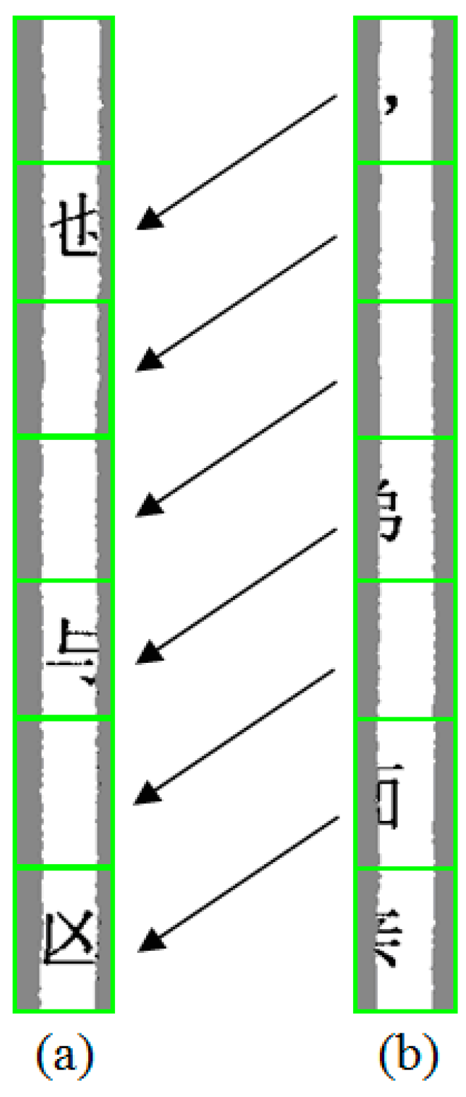
An example of the interrelationships among the leftmost and rightmost pieces from the same page is shown in Figure 5. The character in the first text line of the rightmost piece is a comma, indicating that the content of a sentence is paused rather than ended, and the character in the second text line of the leftmost piece is text, indicating that the content of the previous sentence continues. These two characters are closely related. Additionally, the block in the second text line of the rightmost piece is blank, indicating that the content of a paragraph has ended, and the block in the third text line of the leftmost piece is blank, indicating the indentation of the first text line at the beginning of a new paragraph. These two blanks are also closely related. The relationship between characters and blanks in adjacent horizontal text lines is similar.
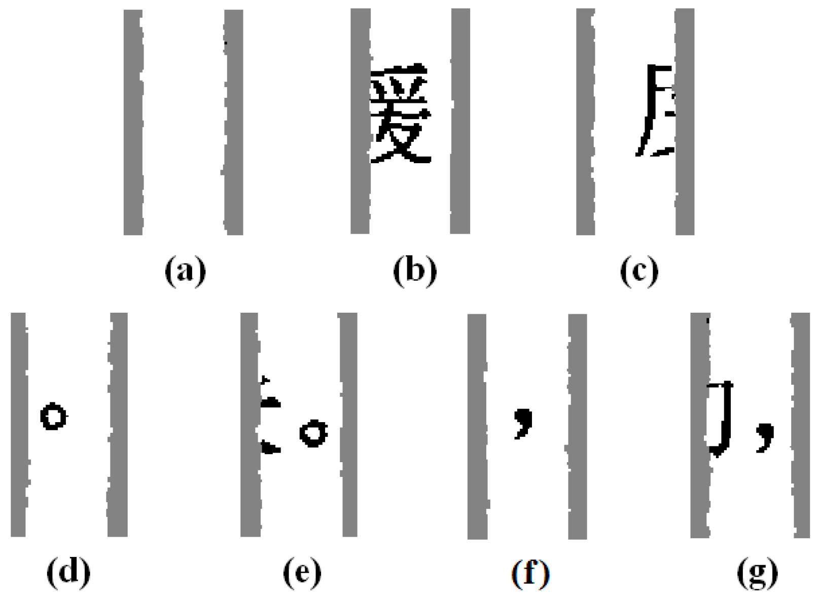
The above analysis indicates that the block in a piece can be divided into text, punctuation (punctuation symbols described in this paper are defined by the General Rules for Punctuation (GB/T 15834-2011) promulgated by the General Administration of Quality Supervision, Inspection and Quarantine of the People’s Republic of China in 2011), and blank spaces according to its attributes. Because different types of punctuation lead to different degrees of relevance between two sentences [21], the block of punctuation must be further divided. Considerable differences are observed in the frequency of punctuation (in particular, the frequency of commas and periods in Chinese documents is much greater than that of other punctuation [22]); therefore, for punctuation in the leftmost piece and the rightmost piece, this paper only considers commas and periods while ignoring other punctuation. Blocks in the leftmost piece and the rightmost piece are divided into four types. A type I block is a blank, as shown in Figure 6a; a type II block only contains text, as shown in Figure 6b,c; a type III block contains a period, as shown in Figure 6d,e; and a type IV block contains a comma, as shown in Figure 6f,g.
Because of restrictions in the document layout, the distributions of these four types of blocks in the leftmost piece and the rightmost piece are different. The type I, type II, type III, and type IV blocks occur in the rightmost piece, whereas only the type I and type II blocks occur in the leftmost piece. We describe the degree of correlation of a block in a text line of the rightmost piece and a block in the next text line of the leftmost piece via the probability shown in Table 1.
In Table 1, represents the block type in a text line of the rightmost piece and represents the block type in the next text line of the leftmost piece. Table 1 reflects the probability of occurrence of different types of leftmost blocks for different types of rightmost blocks.
The operation to match the rightmost piece with the leftmost piece is as follows: First, every piece is divided into a series of blocks in the vertical direction. Second, to classify the blocks, the text, periods, commas, and blanks in the blocks are distinguished by the method described in [23]. Third, a rightmost piece is selected arbitrarily, and the matching scores of and all the leftmost pieces are calculated:
where represents the i-th rightmost piece, represents the matching score between the i-th rightmost piece and the j-th leftmost piece, and represents the total number of leftmost pieces. is expressed by the cumulative value of the correlation of the block in the leftmost piece and the block in the rightmost piece.
where represents the number of text lines (number of blocks) in a piece and represents the degree of correlation between the block in the k-th text line of the rightmost piece and the block in the k + 1-th text line of the leftmost piece.
Subsequently, the leftmost piece with the highest matching score to is found; thus, is a leftmost piece that came from the same page as .
where represents the index number corresponding to the leftmost piece.
The above steps are repeated until all the rightmost and leftmost pieces are paired; then, the entire matching algorithm ends.
2.3. Piece Clustering Based on the Regional Division
As a carrier of characters, a document can be divided into several paragraphs according to the content hierarchy, and explicit boundary markers occur between the different paragraphs [24,25]. Different documents lead to different paragraph layouts because of the diverse content [26]. However, in the same document, the paragraph layout in different regions is correlated because of the constraints of the writing format. As a derivative of the document, the piece also has the corresponding attribute of the document; therefore, the layouts of pieces from different pages are different, while the layouts of pieces from the same page are relevant.
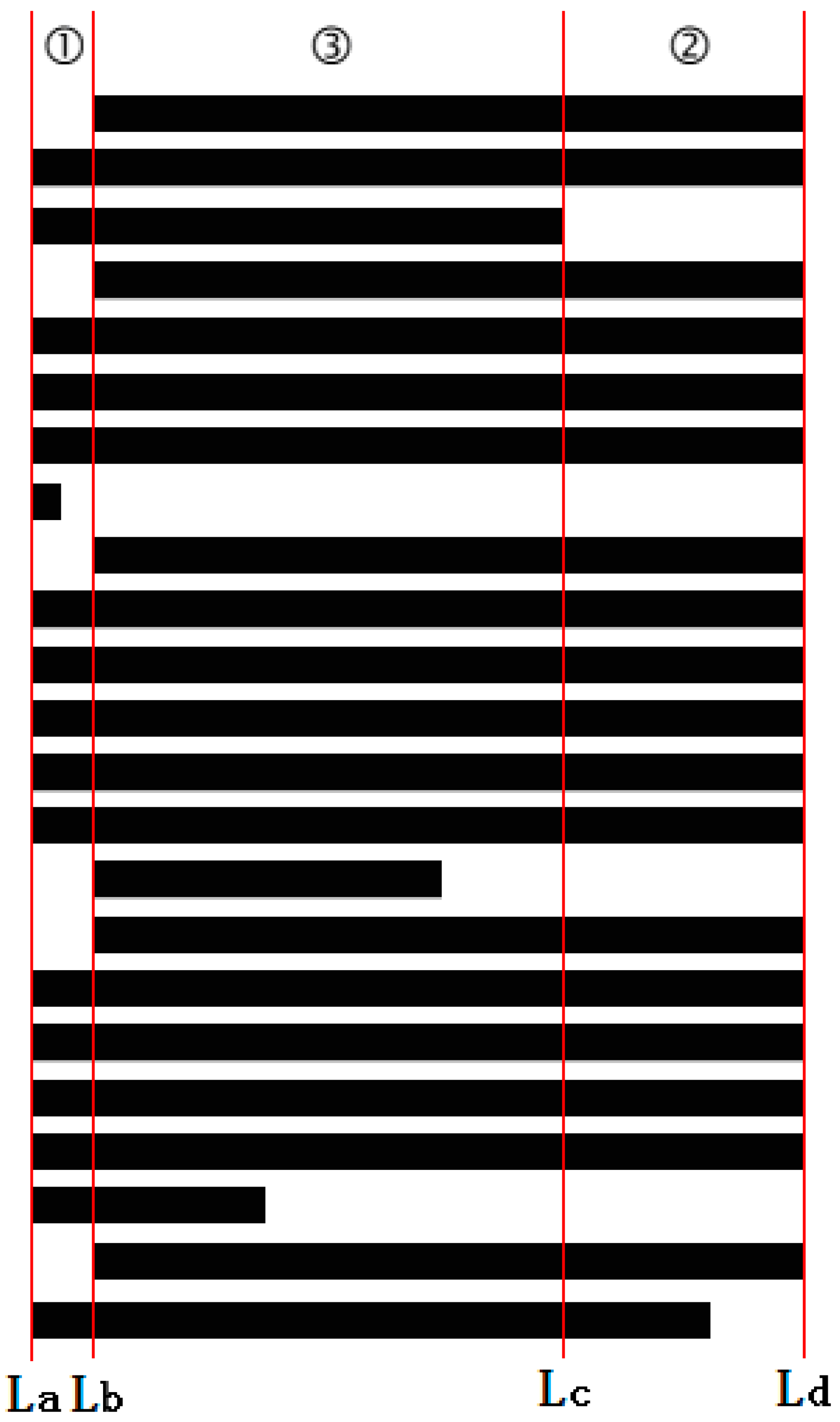
Based on the above analysis, a page of a shredded document is divided into three areas, as shown in Figure 7. The beginning of each paragraph in the document is area 1; the end of each paragraph in the document is area 2; and the middle region of the document is area 3. The contents marked by black represent text or punctuation, and the contents marked by white represent blank spaces. The red line indicates the leftmost piece, the red line indicates the critical piece between area 1 and area 3, the red line indicates the critical piece between area 3 and area 2, and the red line indicates the rightmost piece.
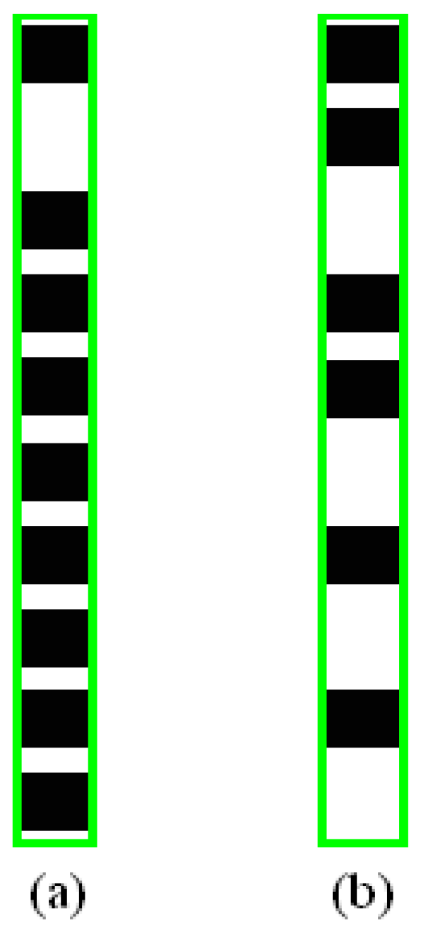
For real pieces, the range of the three areas in a document is not fixed because the paragraph layouts of different documents are not the same, which means that the positions of and vary among different documents. As shown in Figure 8, to clearly divide the regions where the pieces belong, we divide the pieces (excluding the leftmost and rightmost pieces) into dense pieces and sparse pieces with a blank line ratio because the character distribution in a document appears to be “dense in the middle, sparse on both sides” (because of the presence of blanks at the beginning and end of a paragraph).
where represents the total number of blocks along the vertical direction of a piece (the total number of text lines in a piece) and represents the total number of blank blocks in the vertical direction of a piece (the total number of blank lines in a piece). A shred with a value of less than 0.15 is defined as a dense piece, and a shred with a value of greater than or equal to 0.15 is defined as a sparse piece.
In general, the dense pieces are located in area 3 of a document, while the sparse pieces are located in areas 1 and 2. The sparse pieces associated with are located in area 1, and the sparse pieces associated with are located in area 2. Because and are in critical positions, both dense and sparse pieces can occur. In this paper, is a dense piece and is a sparse piece. Note that there are differences in the number of dense and sparse pieces from different pages.
In this paper, pieces are clustered based on regional divisions. The algorithm is composed of three parts: piece clustering in area 1, piece clustering in area 2, and piece clustering in area 3. The system flowchart is shown in Figure 9.
2.3.1. Piece Clustering in Area 1
From the layout, the pieces in area 1 are located on the left side of the document. Because area 1 is affected by the indentation, the range of area 1 in the horizontal direction is narrow; therefore, the area contains few shreds. In addition, these pieces are closely related because the shredded characters in the horizontal direction are correlated.
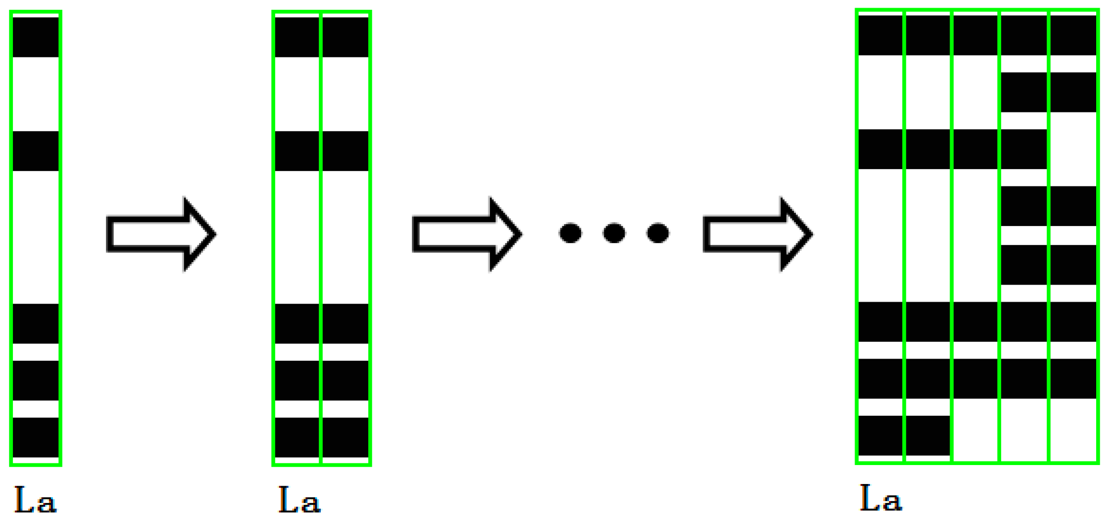
Based on the above analysis, we use the leftmost piece , which is obtained in Section 2.2, as the starting point of clustering in area 1, and use the basic matching algorithm proposed in reference [20], which utilizes the number of mismatched combinations and the relevance between pieces to measure the matching degree of pieces, to perform piece matching from left to right. As shown in Figure 10, is the starting point and the pieces on the right side of are agglomerated gradually.
The clustering operations proceed as follows: First, one shred (i.e., the leftmost piece in the i-th page of the document) is chosen randomly from all the leftmost pieces obtained in Section 2.2 and is used as the starting point. Second, by applying the basic matching algorithm (proposed in [19]) from left to right, a piece is found that matches in the set that includes all the dense and sparse pieces to be tested. Third, the two matched pieces are regarded as a whole, and the basic matching algorithm is used to match them with other pieces. The above steps are repeated until two dense pieces are continuously matched, and the assembly process that begins with is completed. We use the second matched dense piece as the critical piece . Then, the assembly process that begins with the other leftmost piece is completed by the same method. When all the assembly processes are complete, piece clustering in area 1 terminates.
As this matching process proceeds, the number of pieces in set is gradually reduced. In addition, to incorporate the influence of document skew (because people do not place documents vertically into a shredder) on the blank and character distribution in the shreds, two continuous dense pieces are set as the clustering end condition in this paper and the second dense piece (rather than the first dense piece) is set as a critical shred between area 1 and area 3.
2.3.2. Piece Clustering in Area 2
The pieces in area 2 are located on the right side of an entire document. Because the usual Chinese document typography includes a horizontal arrangement in which words start from the left side [27], area 2 mainly reflects the layout of the ends of paragraphs. As shown in Figure 11, three types of characters (words and punctuation) and blank distributions are observed in the horizontal direction at area 2. The first type is “from character to character”, which means that the paragraph does not end or the paragraph ends just at the rightmost area of a document; therefore, the entire line in area 2 consists of characters (see the regions surrounded by a red border in Figure 11). The second type is the “from blank to blank”, which means that the paragraph has ended in the front area; therefore, the entire region in area 2 is blank (see the regions surrounded by a blue border in Figure 11). The third type is the “from character to blank”, which means that the paragraph ends in area 2 and the left side of the line is a character; therefore, the right side is blank (see the regions surrounded by a green border in Figure 11).
In Figure 11, because the position of the end of a paragraph is indeterminate, we use the rightmost part of area 2 in a document as the starting point, and from right to left, the blanks may not be continuous, although the characters must be continuous. Therefore, for the shreds in area 2, this paper proposes a clustering algorithm based on the line position of characters (LPC algorithm). Flowchart of LPC algorithm is shown in Figure 12, and each step of LPC algorithm is described in detail as follows.
| LPC (line position of characters) Algorithm: |
|
It should be noted that the number of character blocks contained in the sparse pieces clustered with is greater than or equal to the number of character blocks contained in , as shown in Figure 13, because in area 2 of a document, the rightmost character distribution is the sparsest, and as the position moves to the left, the sparseness gradually decreases.
In the set of rightmost pieces, the probability that all character lines in a piece are contained by another piece is small, as shown in Equation (8). Therefore, the pieces from the different pages of documents in area 2 are unlikely to be misclassified, and the clustering method using the line position of characters is reliable.
where is the total number of blocks in a piece, is the number of character blocks in a piece, and , , represents the combination value of and .
2.3.3. Piece Clustering in Area 3
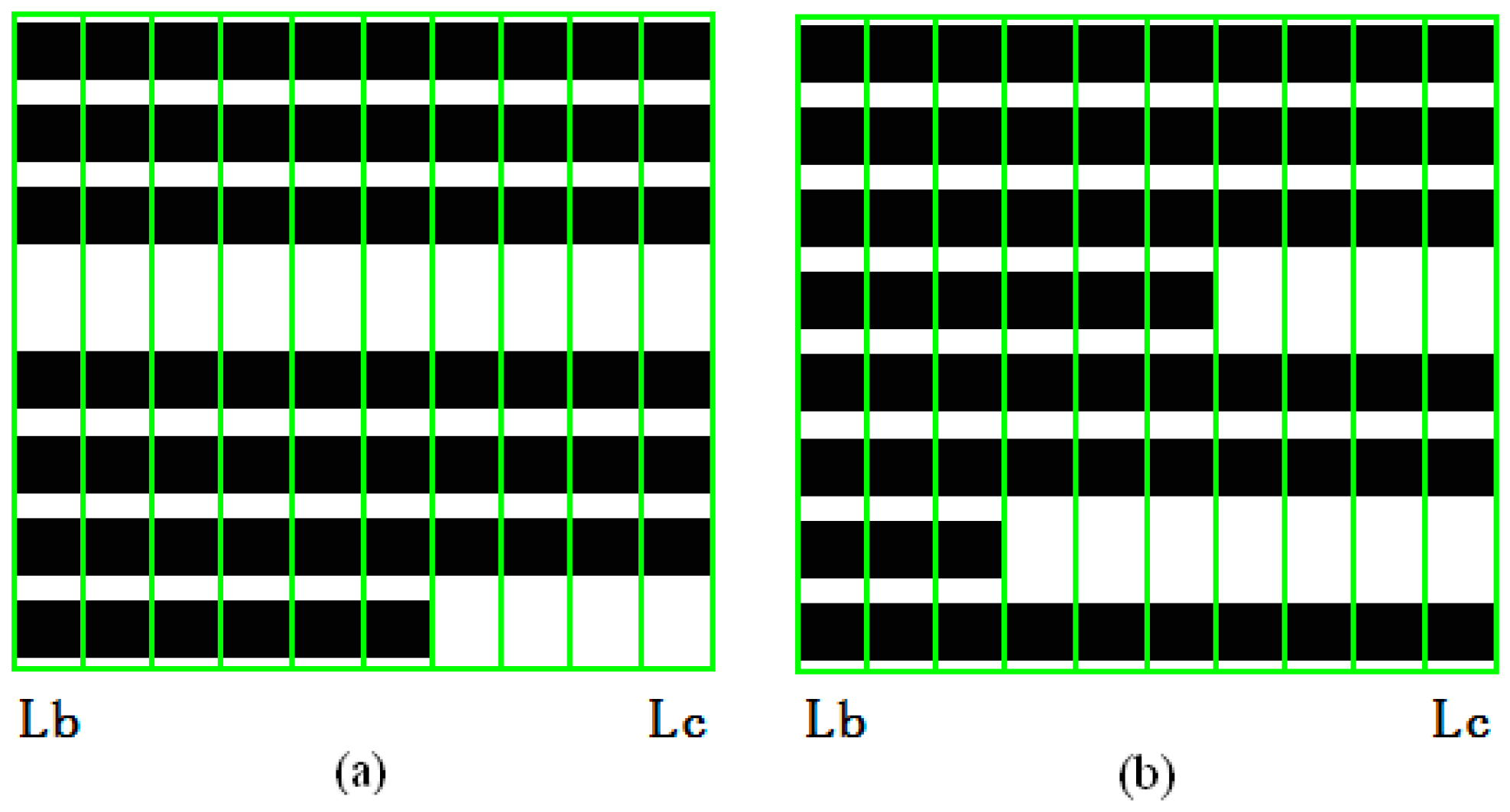
For area 3 of a document, the left and right boundary pieces are and , respectively, and these pieces on the same page can be obtained from Section 2.3.1 and Section 2.3.2. From the view of boundary shreds, the pieces in area 3 can be divided into two cases. In the first case, the boundary pieces and have blank blocks in the same line, as shown in Figure 14a; and in the second case, the boundary pieces and do not have blank blocks in the same line, as shown in Figure 14b.
Based on the above analysis, this paper proposes a double-pronged attack strategy and gradual agglomeration strategy to achieve clustering.
In the double-pronged attack strategy, which is applied for Figure 14a, because the text and punctuation in the paragraph are continuous in the horizontal direction instead of intermittent [29], when the two boundary pieces and from the same page have one or more blank blocks in the same line, then the paragraphs in these line positions have ended; therefore, all pieces in area 3 of this page of a document are also blank blocks in these line positions. If the pieces have the same blank blocks with both boundary shreds, then they are in the same cluster as two boundary shreds; otherwise, they are not.
In the gradual agglomeration strategy, which is applied for Figure 14b, because the end of a paragraph is random, the pieces in area 3 and both boundary shreds lack uniform distributions of characters and blanks. The interrelationships of the text structures (blocks) in the adjacent pieces are used to gradually match the pieces of area 3 with the boundary shred. Using the basic matching algorithm proposed in reference [20], the boundary shred is taken as a starting point; then, the pieces in area 3 are gradually absorbed into the cluster via matching from right to left. When the matching degree of pieces reaches a threshold, the clustering is complete.
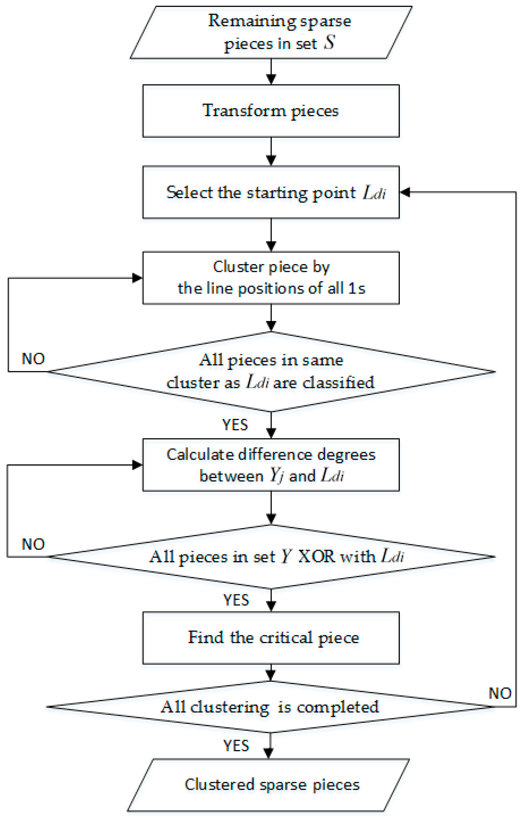
The following steps constitute the clustering algorithm, which uses the blanks on the same line to realize piece clustering in area 3. We refer to this algorithm as the “blanks on the same line” (BSL) algorithm, and flowchart of BSL algorithm is shown in Figure 15.
| BSL (blanks on the same line) Algorithm: |
|
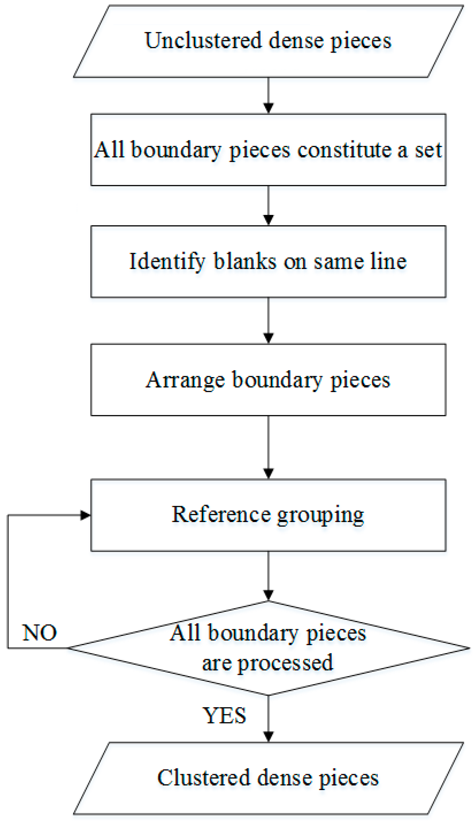
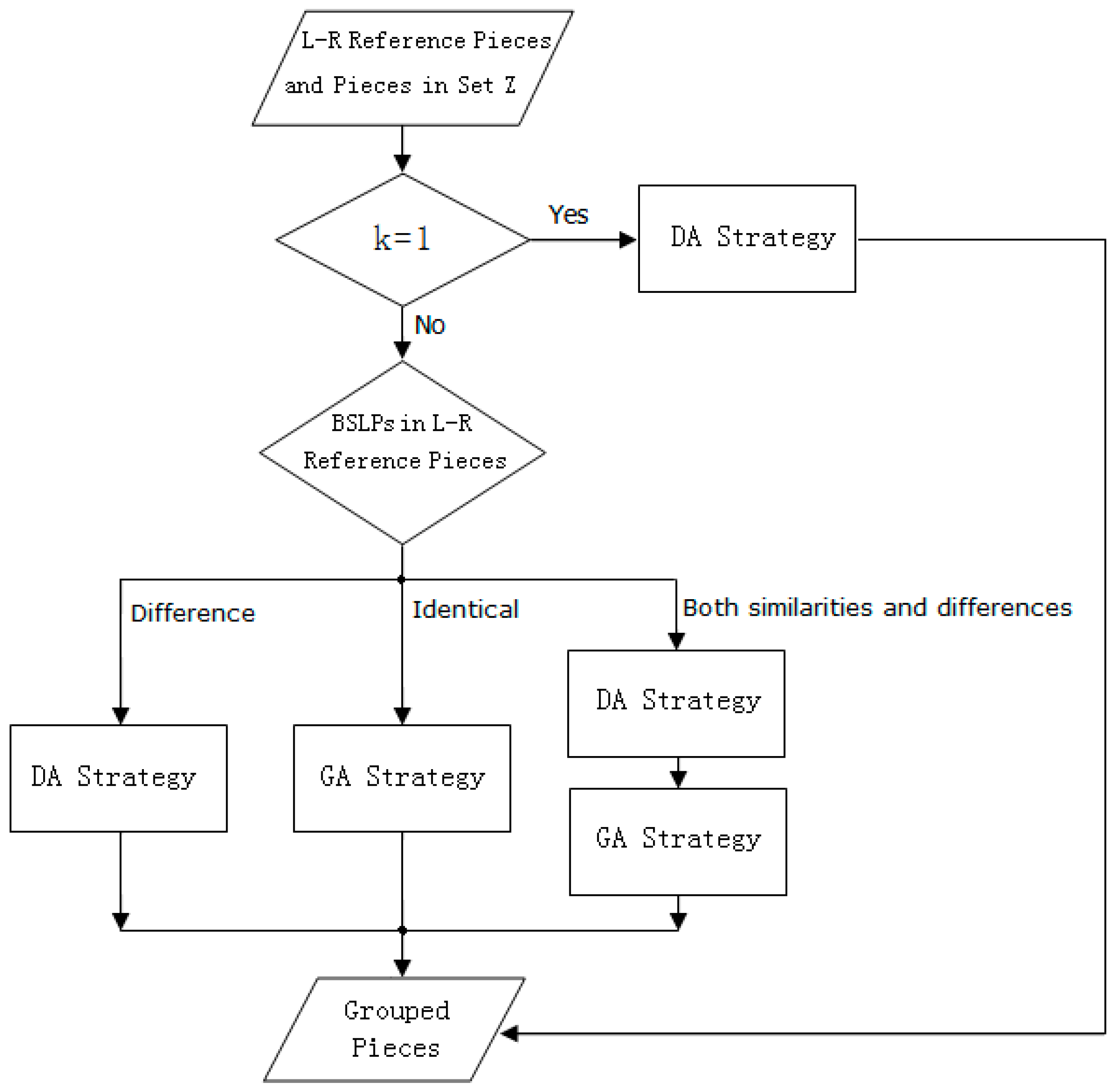
In the above algorithm, the reference grouping is an important part of realizing clustering, and its algorithm flowchart is shown in Figure 16. When the pieces in set are clustered, the number of pairs of left-right reference pieces (L-R reference pieces), i.e., , needs to be determined first. If , then the shreds are clustered using the double-pronged attack strategy (DA Strategy). If , then there are several pairs of L-R reference pieces, and according to the relationship of blanks on the same line position (BSLP) in different pairs of L-R reference pieces, we divide the pairs into three cases. For the first case, the BSLPs in pairs of left-right reference pieces are different. We take each pair of left-right reference pieces as the reference and use the DA Strategy to group the shreds. For the second case, the BSLPs in pairs of left-right reference pieces are identical. We take each pair of left-right reference pieces as the reference and use the gradual agglomeration strategy (GA Strategy) to group the shreds. For the third case, in pairs of left-right reference pieces, the BSLPs in pairs of the pieces are different, and the BSLPs in pairs of the pieces are identical, where . First, we take pairs of left-right reference pieces as the reference and use the DA Strategy to group the shreds. Second, we take pairs of left-right reference pieces as the reference and use the GA Strategy to group the shreds.
It should be noted that if a BSL is not observed in a pair of left-right reference pieces, we use the GA Strategy to group the shreds.
3. Experimental Results and Discussion
The method proposed in this paper is tested with real pieces. Ten-page documents from a long file are randomly selected as the original dataset. In the dataset, the paper size is A4, the paper color is white, and the type of paper is blank paper not squared paper. All documents are edited using Microsoft Office Word (Microsoft Corporation, Redmond, WA, USA) following the unified format: the font is Song style, the character color is black, the character size is small four, and the line spacing is 1.5. All documents are shredded by a Sunwood ST9290 shredder (Sunwood Holding Group Co., Ltd., Yuhuan, Zhejiang, China), and 462 pieces are produced in total (excluding the blank shreds); each piece has a width of 3 mm. The experiment is executed on a computer (Mingsu-U2, Ningdong Electronic Technology Co., Ltd, Guangzhou, Guangdong, China) with an Intel Core 2 3.0 GHz CPU, 4 GB memory, and a 500 GB hard disk.
In the original dataset (the dataset S1 in supplementary), the 10-page documents are designated A to J, and all shreds in each page document are numbered in sequence; for example, the original index numbers of the pieces in document A range from A1 to A46. In the actual test, because shreds from different pages are mixed together and the shred sequences are disrupted, the pieces are renumbered from 1 to 462 to constitute the test dataset. In the experimental process, the test index numbers of shreds are visible, and the original index numbers of shreds are invisible.
3.1. Clustering Number Results
The clustering numbers of the test dataset can be obtained by the process described in Section 2.1. The method for calculating the clustering number must first identify all the leftmost and rightmost pieces in the dataset. The size of in Formula (1) is the basis for judging whether a shred is the leftmost piece and the size of in Formula (2) is the basis for judging whether a shred is the rightmost piece. Therefore, based on the detection results for 100 pages of documents in the experiment, including 4668 shreds, we set the dual thresholds of to and , and the dual thresholds of to and . The identification results of the leftmost and rightmost pieces in the test dataset are shown in Figure 17 and Figure 18, respectively.
Figure 17 shows the identification results for the leftmost pieces. The values of different shreds in Figure 17 indicate that there are 10 shreds in the range but none in the range , which means that the number of leftmost pieces is 10 and can be obtained without manual assistance. Figure 18 shows the identification results for the rightmost pieces. Similar to the above analysis, we know that the number of rightmost pieces is 10. A comparison with the original index numbers of shreds shows that these 20 shreds are the leftmost and rightmost pieces. Therefore, although the identification of actual shreds is affected by noise interference at the edge of a piece and classification errors, the method proposed in Section 2.1 can effectively identify the leftmost and rightmost pieces. Based on the number of leftmost and rightmost pieces, the clustering number of shreds in the test dataset is calculated as 10.
3.2. Results for the Starting Points of Clusters
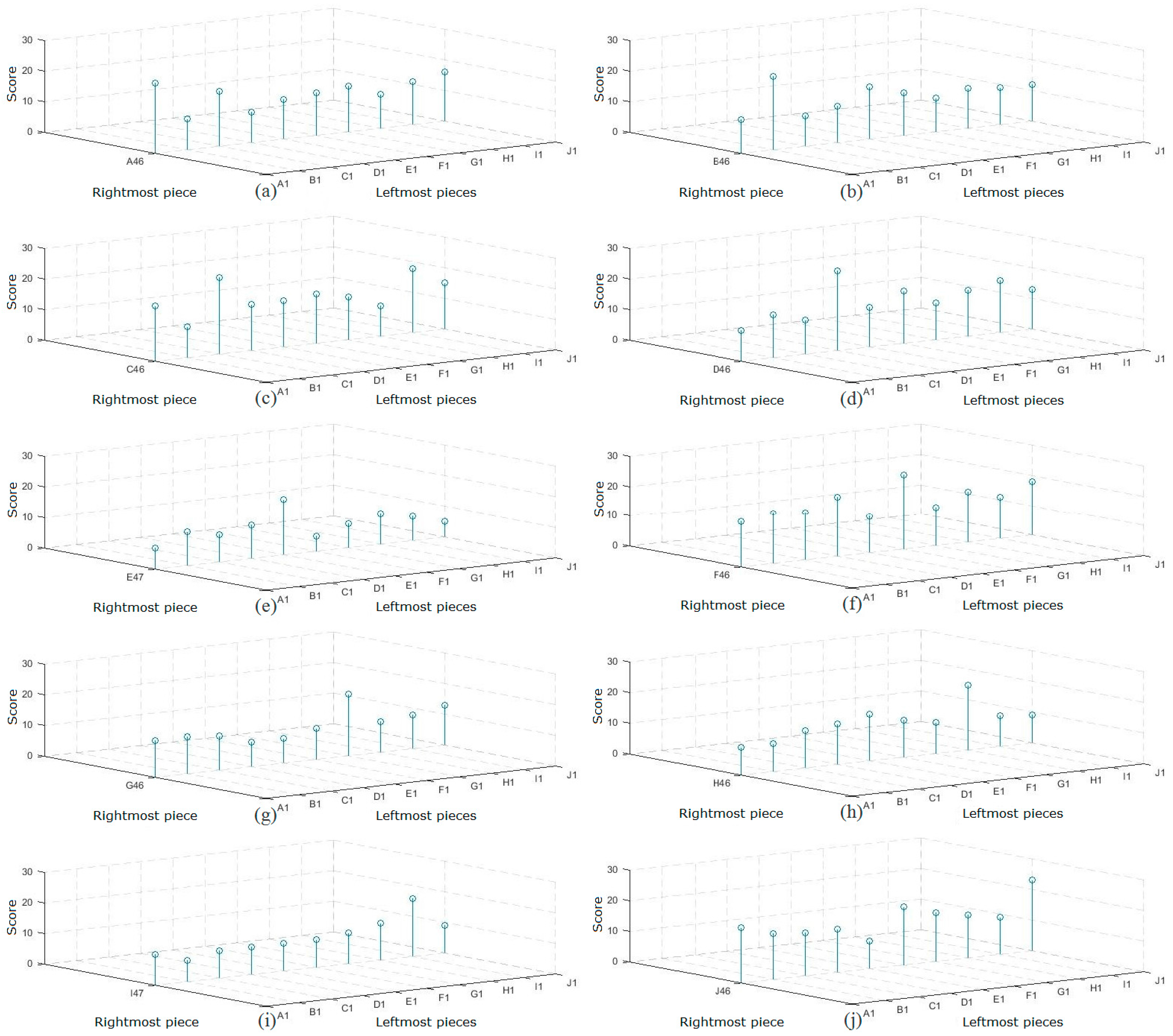
For the leftmost and rightmost pieces obtained in Section 2.1, we use the method proposed in Section 2.2 to calculate matching scores between each rightmost and all leftmost pieces, respectively. The results are shown in Figure 19. The matching score between the rightmost and leftmost pieces from the same page is greater than the matching score between the rightmost and leftmost pieces from different pages. Although the matching scores for several pages are not high (the loss of character information and misjudgment of a few blocks by noise affects the matching scores between shreds), as shown in Figure 19e, the final matching result is not impeded. Because the misjudged blocks are in the minority, the matching scores between the rightmost and leftmost pieces from the same page are clearly higher than the matching scores of other shreds.
To clarify the matching relationship of the rightmost and leftmost pieces, we use the original index number instead of the test index number to mark each piece.
3.3. Results of Piece Clustering Based on Regional Divisions
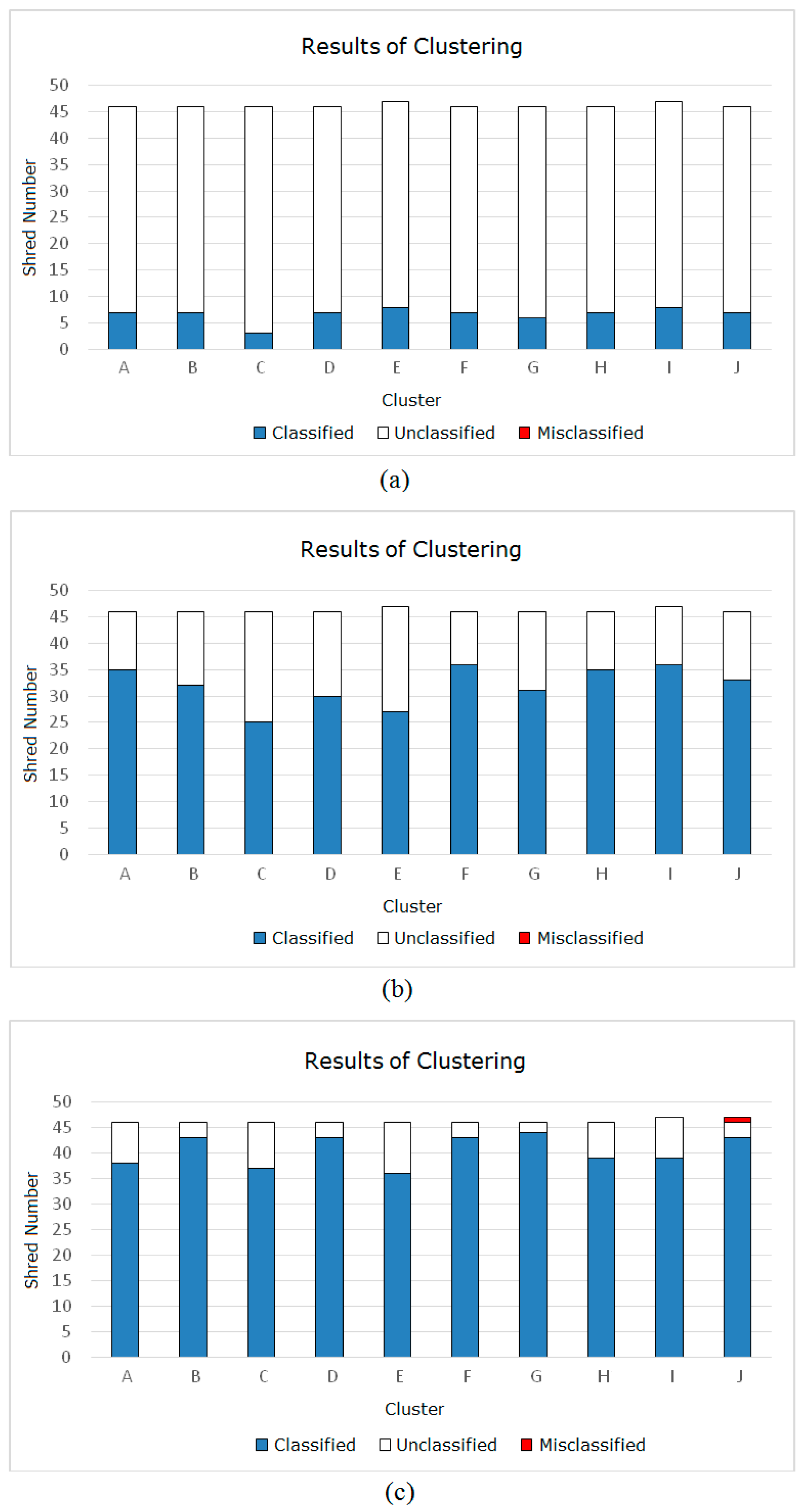
Based on the pairing of rightmost pieces with leftmost pieces described in Section 2.2, we adopt the method proposed in Section 2.3 to cluster the shreds in the test dataset. Figure 20a–c indicate the clustering results of each stage of Section 2.3. Figure 20a represents the clustering results after Section 2.3.1 processing; Figure 20b represents the clustering results after Section 2.3.2 processing; and Figure 20c represents the clustering results after Section 2.3.3 processing. To clearly reflect the clustering results of each stage, we use a histogram to describe the piece clustering process in each page of the document.
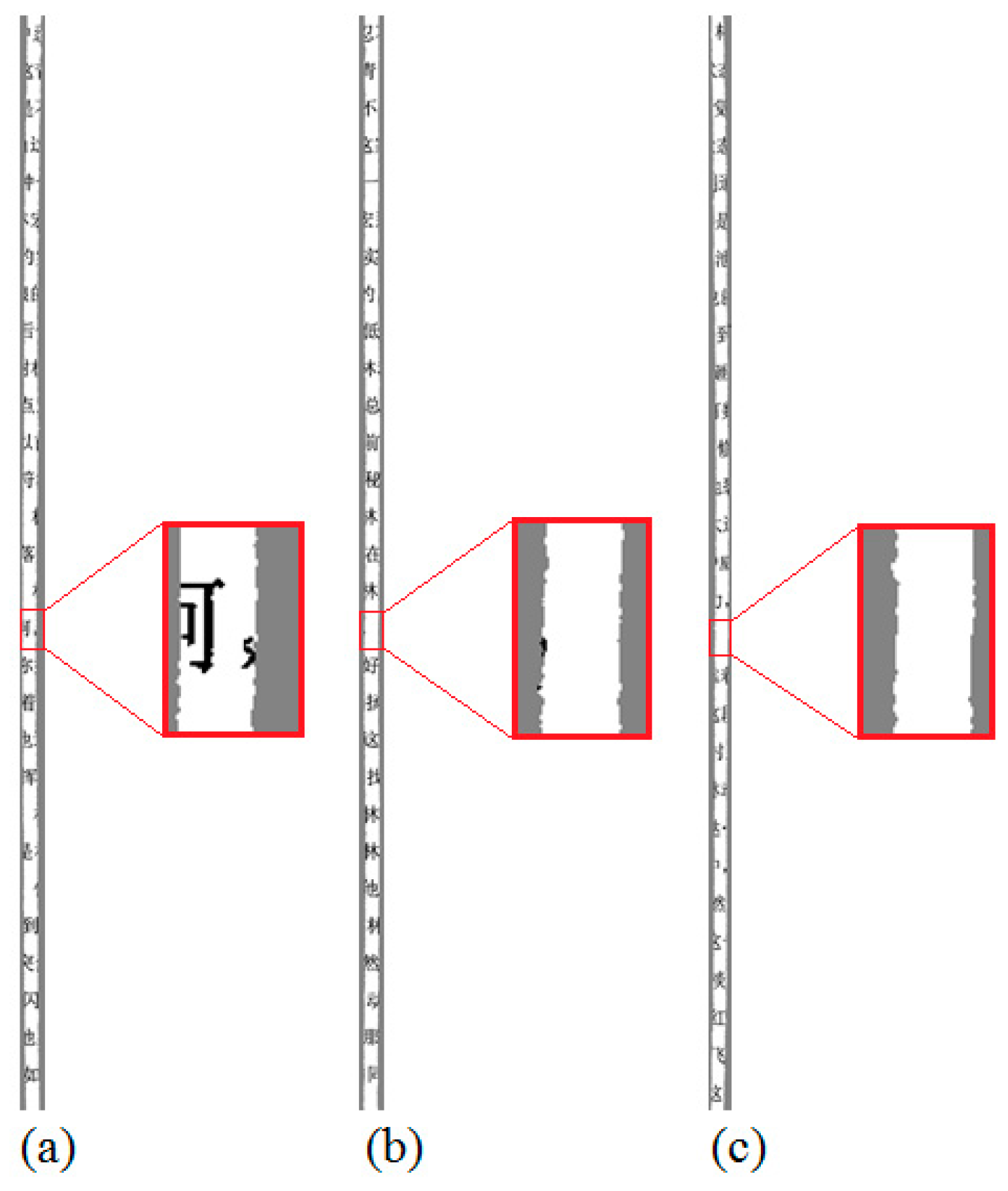
As shown in Figure 20, the number of shreds in each cluster gradually increases in stepwise fashion during clustering. The number of shreds in each cluster in area 1 is low, as shown in Figure 20a, while the number of shreds in each cluster in area 2 is higher, as shown in Figure 20b. This distribution is consistent with the actual layout of the document. In addition, misclassified shreds were not generated during these two parts of the clustering process, which shows that the method is effective. One misclassified shred occurred in Section 2.3.3, as shown in Figure 20c, and the cause of this misclassified shred is shown in Figure 21. Because the misclassified shred (the original index number is E11) contains only a small fraction of a comma in the 17th line (the comma is split into two pieces), it causes a block that should include punctuation to be judged as a blank block; however, this misjudgment leads to a shred E11 where the dense pieces in cluster J have blanks on the same line. Therefore, when the dense pieces in cluster J are clustered under the DA Strategy, shred E11 is incorrectly classified into cluster J.
However, 56 shreds (12.12% in total) remain unclassified, as shown in Figure 20c, which illustrates that under conditions with various real shreds, the method proposed in this paper has certain deficiencies; thus, further improvements must be made to classify the residual shreds.
3.4. Treatment of Residual Shreds
The residual shreds are composed of 44 sparse pieces and 12 dense pieces. First, we analyze the sparse pieces in the majority and find that the reason why they are not clustered is due to misjudgments of block type caused primarily by noise at the edge of a shred and a small part of a word or a punctuation mark in a shred (caused by shredder slicing), as shown in Figure 22.
Although differences may occur in the layout of a character and a blank between different shreds, neighboring shreds from the same page usually present a similar layout [28]. Therefore, even if a few blocks in the shred are misjudged, the layouts of the neighbor shreds from the same page are still closely related. Based on the above analysis, we use the total number of the same type of blocks between two shreds to assess the residual sparse pieces. As shown in Figure 23, a line-by-line comparison of the blocks between two shreds is executed along the vertical direction. If the types of two blocks are the same, then the line is marked as ; otherwise, it is marked as . The sum of is the total number of the same types of blocks , and can reflect the neighborhood degree of two shreds.
The specific process of residual sparse piece clustering is as follows.
A sparse piece is selected randomly from the set of residual sparse pieces .
where represents the i-th residual sparse piece and indicates the total number of residual sparse pieces.
The total number of the same types of blocks between and shreds that have been classified is calculated separately, and the calculation results form a set :
where represents the total number of the same types of blocks between the i-th residual sparse piece and the j-th shred that has been classified; and indicates the total number of shreds that have been classified.
Then, we search for the shred , which has the highest total number of the same types of blocks between and itself:
where represents the test index number of the corresponding shred.
If the value of is unique, then and are considered to be in the same cluster and is incorporated into the same cluster as ; however, if has values (), then the set must be evaluated. consists of candidate shreds:
where represents the x-th candidate shred. If all shreds in are from the same cluster, then is incorporated into the cluster, whereas if the shreds in are from different clusters, then is marked as an unclassifiable shred.
The same method is used to evaluate the other residual sparse pieces until all residual sparse pieces have been processed. Then, the algorithm is complete.
Experiments demonstrate that these improvements are effective. Figure 24 presents the results of processing residual sparse pieces. All residual sparse pieces are incorporated into the correct clusters, and the shreds that are not yet classified are dense pieces. These findings illustrate that the improvements fully exploit the relevance between neighbor pieces, correct for the negative effect of a few blocks misjudged in the original method, and further improve the accuracy of piece clustering.
Second, the residual dense pieces are not classified because certain factors, such as information loss at the edge of a shred and classifier error, affect these shreds when they are clustered according to the GA Strategy. Because of these effects, the shreds are unable to meet the match conditions; thus, they remain unclassified. In addition, because there are many characters and few blanks in a dense piece, the dense pieces from different pages often have the same or similar layouts. Therefore, the method of processing residual sparse pieces does not effectively manage these shreds. Ultimately, 12 dense pieces failed to cluster.
3.5. Summary
After performing the processing described in Section 3.1 to Section 3.4, the clustering results in the test dataset are obtained, as shown in Table 2. The average accuracy of clustering is 97.19% (449/462), 12 shreds are not classified, and one shred is misclassified. These results show that the clustering method proposed in this paper has a high accuracy and a low error rate. Moreover, for homologous pieces that appear indistinguishable, the method proposed in this paper can fully exploit their internal relationships and differences to achieve effective clustering. Although a shortage of shred processing occurs in area 3 of a document, considering the complexity of real shreds, which are affected by noise interference, information loss, and other factors, the clustering results of Table 2 are satisfactory. Additionally, from the point of view of time complexity, the complexity of our algorithm in various stages is not high, with the exception of the process of Section 2.1. The time consumption of this algorithm is acceptable. The time complexity is in Section 2.1 (process of computing the clustering number). Because the training and testing of the classifier for recognizing five different types of blocks in shreds is very time-consuming. The time complexity is in Section 2.2 (process of identifying the starting point of clusters). Since the number of shreds that are processed in this stage is substantially less than the total number of shreds, the time consumption in this stage is minimal. The time complexity is in Section 2.3 (process of achieving piece clustering based on the regional division). In this stage, the complexity of the piece clustering in area 1 and area 3 is greater than the complexity of the piece clustering in area 2.
Additionally, to clearly demonstrate the clustering effect of our method, we employ k-means clustering and hierarchical clustering to test the dataset based on the features of the paragraph layout proposed in this paper. We compared the clustering effect of these two methods with the method proposed in this paper.
We use the common clustering evaluation indexes—purity and silhouette coefficient—as the standards of evaluation. the expression of purity [7] is expressed as:
where indicates purity, indicates the number of clusters, indicates the number of predefined classes, indicates the i-th cluster, and indicates the j-th class.
The expression of silhouette coefficients is expressed as:
where indicates Silhouette coefficient, indicates the number of clustered pieces, indicates the average dissimilarity of the i-th piece with all other pieces within the same cluster, indicates the lowest average dissimilarity of the i-th piece to any other cluster, of which the i-th piece is not a member.
Table 3 shows the clustering effect of different algorithms. The clustering number of k-means clustering is ten. Because the initialization of k-means clustering is random, the purity and silhouette coefficient are the averaging results of 10,000 runs. The clustering number of hierarchical clustering is ten. We use the minimum variance algorithm to create a hierarchical cluster tree in the process of clustering.
As shown in Table 3, compared with other two methods, the method proposed in this paper has obvious advantages in terms of the clustering effect. This is because, at the beginning of the clustering, our method can accurately obtain the starting points of clusters (namely the leftmost and the rightmost pieces from the same page), and these starting points can provide clear guidance for the clustering of other pieces. Additionally, we fully mine the document property of the pieces, and the pieces in different areas are distinguished and associated effectively based on the feature of paragraph layout. Meanwhile, according to the similarity of adjacent pieces in the layout, the interference of individual blocks is suppressed in clustering by using the total number of the same types of blocks. The clustering effect is obviously improved. From the evaluation results, the purity of our method is very high, and the silhouette coefficient is not very high. It is because that the paragraph layouts in different areas of a document are different, and the paragraph layouts in the same area of a document are similar. Accordingly, for a cluster of pieces from a document, there is a high similarity between pieces in the same area, and the similarity between pieces in different areas is not high. The silhouette coefficient uses the similarity of pieces as an important basis for evaluating clustering results in the range of an entire cluster, and it does not adequately reflect the similarity of homologous pieces in a small range. Thus the silhouette coefficient of our method is not very high. For the k-means clustering, the algorithm only uses the layout similarity of characters and blanks to cluster, but it ignores the differences and correlations between pieces in different areas of a page. Thus the pieces from different pages are clustered because of the similar layout, and the separations between different clusters are not high. Moreover, initial centers of clusters that are randomly selected also have an influence on the clustering. The clustering effect of the k-means algorithm is not good, its purity is 67.72%, and its silhouette coefficient is 0.4158. For the hierarchical clustering, although its purity and silhouette coefficient are higher than the k-means, it only realizes clustering based on the layout similarity between pieces, and it does not consider the differences and correlations between pieces from the perspective of the overall document layout, which means that some pieces that came from a page are divided into different clusters because of the different layouts. Therefore, the clustering effect of the hierarchical algorithm is not satisfactory.
4. Conclusions
This paper presents a novel clustering method for Chinese homologous pieces that are difficult to distinguish visually. The pieces are clustered by three steps: computing the clustering number, identifying the starting point of clusters, and achieving piece clustering based on the regional division. In the step of computing the clustering number, based on the distribution features of characters in the piece, the leftmost and rightmost pieces in the documents are recognized, and the clustering number is calculated. In the step of identifying the starting point of clusters, this paper employs the correlation of syntax in adjacent text lines, and the leftmost piece and the rightmost piece which come from the same page are exactly matched. In the step of achieving piece clustering based on the regional division, according to the document layout, the pieces are distinguished in different areas of the document, and piece clustering is achieved by the correlation among pieces in different areas. The experimental results show that the proposed method can effectively achieve the clustering of real pieces. Moreover, this method lays the foundation for the resolution of homologous shredded document recovery.
It is worthy to mention that although this paper addresses shredded plain text documents, it still has an application value for the shredded documents with figures and images. In contrast to homologous pieces in the plain text document (the pieces are very similar with regard to content, and a lack of effective feature distinguishes the pieces), the shredded documents with figures and images contain easily extractable features and achieve clustering because the figures and images have potential differences with regard to size and position in real documents. However, document is different from photograph after all. Characters take the primary position in a document. The distribution of characters in different areas of a document remains dense and sparse, a correlation exists among characters in different areas, and the paragraph layout feature of a document remains in the pieces. Thus, we can also apply the method proposed in this paper to process the shredded documents with figures and images. Because figures and images are added to a document, the total relevance of the characters of the pieces in the horizontal direction is weakened, and it has a certain extent effect on piece clustering. The features of figures and images can be used to easily distinguish the pieces, and they can promote the realization of piece clustering. We need extensive research toward documents with figures and images, which will also be a major direction in our future research.
In future studies, we will investigate homologous clustering, which contains images and tables based on the solution for the shredded plain text document in this paper. We expect to employ a technical method to solve the question of piece clustering based on multi-page documents. Considering that the documents processed in this paper are Chinese documents and that the Chinese language has a text structure that is similar to Vietnamese and Japanese, we will attempt to apply the method proposed in this paper to the piece clustering of documents in these two languages in future studies. From a broader point of view, although the languages in different countries differ, many similarities exist in the paragraph layout among documents in different languages. The cornerstones of the algorithm proposed in this paper exist. Thus, if the idea of this paper is combined with other methods, it will help researchers solve the piece clustering problem of different language documents. Additionally, there are differences in the pieces produced by a shredder because of different cutting methods. This paper addresses strip-cut shredded documents; however, whether the proposed method is still valid for cross-cut shredded documents requires further testing.
Supplementary Materials
The following are available online at https://www.mdpi.com/2076-3417/7/9/951/s1, Dataset S1: The original dataset used in the experiment.
Acknowledgments
Support for this program is provided by Xidian University. Additional support has been provided by Xi’an University of Technology. The authors thank Professor Hong Zhu for her valuable suggestions, as well as Siqi Shi and Yang Liu for their comments on the manuscript.
Author Contributions
Nan Xing and Jianqi Zhang conceived and designed the experiments; Nan Xing and Furong Cao performed the experiments; Nan Xing and Pengfei Liu analyzed the data; Furong Cao contributed analysis tools; and Nan Xing wrote the paper.
Conflicts of Interest
The authors declare no conflict of interest.
References
- Butler, P.; Chakraborty, P.; Ramakrishan, N. The Deshredder: A Visual Analytic Approach to Reconstructing Shredded Documents. In Proceedings of the IEEE Conference on Visual Analytics Science and Technology (VAST), Seattle, WA, USA, 14–19 October 2012; IEEE: Washington, DC, USA, 2012; pp. 113–122. [Google Scholar]
- Ukovich, A.; Ramponi, G.; Doulaverakis, H.; Kompatsiaris, Y.; Strintzis, M.G. Shredded Document Reconstruction Using MPEG-7 Standard Descriptors. In Proceedings of the Fourth IEEE International Symposium on Signal Processing and Information Technology, Rome, Italy, 18–21 December 2004; IEEE: Washington, DC, USA, 2012; pp. 334–337. [Google Scholar]
- Sagiroglu, M.S.; Ercil, A. A Texture Based Matching Approach for Automated Assembly of Puzzles. In Proceedings of the 18th International Conference on Pattern Recognition, Hong Kong, China, 20–24 August 2006; IEEE: Washington, DC, USA, 2006; pp. 1036–1041. [Google Scholar]
- Prandtstetter, M. Hybrid Optimization Methods for Warehouse Logistics and the Reconstruction of Destroyed Paper Documents. Ph.D. Thesis, Vienna University of Technology, Vienna, Austria, 2009. [Google Scholar]
- Ukovich, A.; Ramponi, G. Feature extraction and clustering for the computer-aided reconstruction of strip-cut shredded documents. J. Electron. Imaging 2008, 17, 013008. [Google Scholar] [CrossRef]
- Ukovich, A. Image Processing for Security Applications: Document Reconstruction and Video Enhancement. Ph.D. Thesis, University of Trieste, Trieste, Italy, March 2007. [Google Scholar]
- Ukovich, A.; Zacchigna, A.; Ramponi, G.; Schoier, G. Using Clustering for Document Reconstruction. In Proceedings of the IS&T/SPIE Electronic Imaging—Image Processing: Algorithms and Systems, Neural Networks, and Machine Learning, San Jose, CA, USA, 16–17 January 2006; SPIE: Bellingham, WA, USA, 2006; pp. 168–179. [Google Scholar]
- Wang, Y.; Ji, D.C. A Two-Stage Approach for Reconstruction of Cross-Cut Shredded Text Documents. In Proceedings of the Tenth International Conference on Computational Intelligence and Security, Kunming, China, 15–16 November 2014; IEEE: Washington, DC, USA, 2014; pp. 12–16. [Google Scholar]
- Sleit, A.; Massad, Y.; Musaddaq, M. An alternative clustering approach for reconstructing cross cut shredded text documents. Telecommun. Syst. 2013, 52, 1491–1501. [Google Scholar] [CrossRef]
- Richter, F.; Ries, C.X.; Cebron, N.; Lienhart, R. Learning to reassemble shredded documents. IEEE Trans. Multimed. 2013, 15, 582–593. [Google Scholar] [CrossRef]
- Lei, W. Features for the reconstruction of cross cut shredded Chinese text documents. Pak. J. Stat. 2014, 30, 1487–1494. [Google Scholar]
- Guo, S.; Lao, S.; Guo, J.; Xiang, H. A Semi-Automatic Solution Archive for Cross-Cut Shredded Text Documents Reconstruction. In Proceedings of the 8th International Conference on Image and Graphics, Tianjin, China, 13–16 August 2015; Springer: Cham, Germany, 2015; pp. 447–461. [Google Scholar]
- Schoier, G. An algorithm for document reconstruction. In Proceedings of the Analysis Modeling of Complex Data in Behavioural and Social Sciences, Anacapri, Italy, 3–4 September 2012; SIS: Roma, Italy, 2012; pp. 1–4. [Google Scholar]
- Diem, M.; Kleber, F.; Sablatnig, R. Document Analysis Applied to Fragments: Feature Set for the Reconstruction of Torn Documents. In Proceedings of the 9th IAPR International Workshop on Document Analysis Systems, Boston, MA, USA, 9–11 June 2010; ACM: New York, NY, USA, 2010; pp. 393–400. [Google Scholar]
- Chanda, S.; Franke, K.; Pal, U. Clustering Document Fragments Using Background Color and Texture Information. In Proceedings of the IS&T/SPIE Electronic Imaging—Document Recognition and Retrieval XIX, Burlingame, CA, USA, 24 Janaury 2012; SPIE: Bellingham, WA, USA, 2012. [Google Scholar]
- Liu, H.; Cao, S.; Yan, S. Automated assembly of shredded pieces from multiple photos. IEEE Trans. Multimed. 2011, 13, 1154–1162. [Google Scholar] [CrossRef]
- Lalitha, K.S.; Sukhendu, D.; Arun, M.; Koshy, V. Graph-Based Clustering for Apictorial Jigsaw Puzzles of Hand Shredded Content-less Pages. In Proceedings of the Eighth International Conference on Intelligent Human Computer Interaction, Pilani, India, 12–13 December 2016; Springer: Cham, Germany, 2016; pp. 135–147. [Google Scholar]
- Du, Q. A Study in Modern Chinese Text Image and Typographic Norms. Ph.D. Thesis, China Central Academy of Fine Arts, Beijing, China, 2014. [Google Scholar]
- De Smet, P.; De Bock, J.; Philips, W. Semiautomatic Reconstruction of Strip-Shredded Documents. In Proceedings of the IS&T/SPIE Electronic Imaging—Image and Video Communications and Processing 2005, San Jose, CA, USA, 18–20 January 2005; SPIE: Bellingham, WA, USA, 2005; pp. 239–248. [Google Scholar]
- Xing, N.; Zhang, J. Graphical-character-based shredded Chinese document reconstruction. Multimed. Tools Appl. 2017, 76, 12871–12891. [Google Scholar] [CrossRef]
- Ding, J. New Standard Based on 2011 Usage of Punctuation. Master’s Thesis, Peking University, Beijing, China, 2011. [Google Scholar]
- Guo, P. Research on the Chinese Punctuation since the 20th Century. Ph.D. Thesis, Central China Normal University, Wuhan, China, 2006. [Google Scholar]
- Xue, W. Extraction and Recognition of Punctuation Marks in Chinese Document Layout. Master’s Thesis, Nanjing University of Science and Technology, Nanjing, China, 2006. [Google Scholar]
- Longacre, R.E. The paragraph as a grammatical unit in discourse and syntax. Syntax Semant. 1979, 12, 115–134. [Google Scholar]
- Hinds, J. Paragraph structure and pronominalization. Pap. Linguist. 1977, 10, 77–99. [Google Scholar] [CrossRef]
- Li, N.; Tian, Y.; Hou, X.; Liang, Q. A discussion relationship between revisable and non-revisable document formats. Acta Electron. Sin. 2008, 36, 128–132. [Google Scholar]
- Wang, D.; Cui, Z.; Ge, L.; Li, Y. The research on visual recognition performance differences between horizontal layout and vertical layout in both English and Chinese characters. Chin. J. Ergon. 2014, 20, 13–17. [Google Scholar]
- Lin, H.-Y.; Fan-Chiang, W.-C. Reconstruction of shredded document based on image feature matching. Expert Syst. Appl. 2012, 39, 3324–3332. [Google Scholar] [CrossRef]
- Jia, Y.-M.; Wu, J. A document processing model supporting multilingual text layout direction. J. Chin. Inf. Process. 2007, 21, 60–66. [Google Scholar]
Figure 1.
Example of homologous pieces. All the pieces in this figure are derived from the same file: (a) and (b) belong to the first page of the document; (c) and (d) belong to the second page of the document; (e) and (f) belong to the third page of the document.
Figure 1.
Example of homologous pieces. All the pieces in this figure are derived from the same file: (a) and (b) belong to the first page of the document; (c) and (d) belong to the second page of the document; (e) and (f) belong to the third page of the document.

Figure 2.
Piece divided into a series of blocks.

Figure 3.
Five types of graphical Chinese characters. The numbers 1, 2, 3, 4, and 5 indicate different types of graphical Chinese characters.
Figure 3.
Five types of graphical Chinese characters. The numbers 1, 2, 3, 4, and 5 indicate different types of graphical Chinese characters.

Figure 4.
Leftmost piece, middle piece, rightmost piece, and their corresponding digital sequences: (a) leftmost piece and (d) corresponding digital sequence; (b) middle piece and (e) corresponding digital sequence; (c) rightmost piece and (f) corresponding digital sequence.
Figure 4.
Leftmost piece, middle piece, rightmost piece, and their corresponding digital sequences: (a) leftmost piece and (d) corresponding digital sequence; (b) middle piece and (e) corresponding digital sequence; (c) rightmost piece and (f) corresponding digital sequence.

Figure 5.
Example of the interrelationships among the leftmost piece and the rightmost piece on the same page: (a) leftmost piece of the document; (b) rightmost piece of the document. The green frame represents the space range of the block in each text line.
Figure 5.
Example of the interrelationships among the leftmost piece and the rightmost piece on the same page: (a) leftmost piece of the document; (b) rightmost piece of the document. The green frame represents the space range of the block in each text line.

Figure 6.
Four types of blocks: (a) a type I block; (b) a type II block; (c) a type II block; (d) a type III block; (e) a type III block; (f) a type IV block; (g) a type IV block.
Figure 6.
Four types of blocks: (a) a type I block; (b) a type II block; (c) a type II block; (d) a type III block; (e) a type III block; (f) a type IV block; (g) a type IV block.

Figure 7.
Page of a document divided into three areas.

Figure 8.
Example of a dense piece and sparse piece: (a) dense piece; (b) sparse piece. The black area represents characters, and the white area represents blank spaces.
Figure 8.
Example of a dense piece and sparse piece: (a) dense piece; (b) sparse piece. The black area represents characters, and the white area represents blank spaces.

Figure 9.
System flowchart of the piece clustering algorithm.

Figure 10.
Process of piece clustering in area 1.

Figure 11.
Different distributions of characters and blanks in area 2.

Figure 12.
Flowchart of LPC (line position of characters) algorithm.

Figure 13.
Comparison of the number of character blocks contained in the pieces of area 2. The red boxes mark the character blocks with the same line position in the different pieces.
Figure 13.
Comparison of the number of character blocks contained in the pieces of area 2. The red boxes mark the character blocks with the same line position in the different pieces.

Figure 14.
Distribution of pieces in area 3 of a document: (a) the boundary pieces and have blank blocks in the same line; (b) the boundary pieces and do not have blank blocks in the same line.
Figure 14.
Distribution of pieces in area 3 of a document: (a) the boundary pieces and have blank blocks in the same line; (b) the boundary pieces and do not have blank blocks in the same line.

Figure 15.
Flowchart of BSL (blanks on the same line) algorithm.

Figure 16.
Algorithm flowchart of reference grouping.

Figure 17.
Identification results for the leftmost pieces. The ordinate represents the value of the proportion in a shred and the abscissa represents the shreds in the test dataset.
Figure 17.
Identification results for the leftmost pieces. The ordinate represents the value of the proportion in a shred and the abscissa represents the shreds in the test dataset.

Figure 18.
Identification results for the rightmost pieces. The ordinate represents the value of the proportion in a shred and the abscissa represents the shreds in the test dataset.
Figure 18.
Identification results for the rightmost pieces. The ordinate represents the value of the proportion in a shred and the abscissa represents the shreds in the test dataset.

Figure 19.
Matching results between each rightmost piece and all leftmost pieces: (a) the rightmost piece in document A and all leftmost pieces; (b) the rightmost piece in document B and all leftmost pieces; (c) the rightmost piece in document C and all leftmost pieces; (d) the rightmost piece in document D and all leftmost pieces; (e) the rightmost piece in document E and all leftmost pieces; (f) the rightmost piece in document F and all leftmost pieces; (g) the rightmost piece in document G and all leftmost pieces; (h) the rightmost piece in document H and all leftmost pieces; (i) the rightmost piece in document I and all leftmost pieces; (j) the rightmost piece in document J and all leftmost pieces.

Figure 20.
Clustering results of each stage of Section 2.3: (a) clustering results after Section 2.3.1 processing; (b) clustering results after Section 2.3.2 processing; (c) clustering results after Section 2.3.1 processing.
Figure 20.
Clustering results of each stage of Section 2.3: (a) clustering results after Section 2.3.1 processing; (b) clustering results after Section 2.3.2 processing; (c) clustering results after Section 2.3.1 processing.

Figure 21.
Causes of misclassified shreds: (a) dense piece E10 adjacent to E11; (b) dense piece E11; (c) one of the dense pieces in cluster J.
Figure 21.
Causes of misclassified shreds: (a) dense piece E10 adjacent to E11; (b) dense piece E11; (c) one of the dense pieces in cluster J.

Figure 22.
Examples of a small part of a word or a punctuation mark in a shred. (a) a small part of a punctuation mark in a shred; (b) a small part of a word in a shred.
Figure 22.
Examples of a small part of a word or a punctuation mark in a shred. (a) a small part of a punctuation mark in a shred; (b) a small part of a word in a shred.

Figure 23.
Total number of the same types of blocks between two shreds.

Figure 24.
Results of processing residual sparse pieces.


Table 1.
Correlation of two blocks in the rightmost piece and the leftmost piece.
| i | Type I | Type II | Type III | Type IV | |
|---|---|---|---|---|---|
| j | |||||
| Type I | 1 | 0 | 0.5 | 0 | |
| Type II | 0 | 1 | 0.5 | 1 | |
Table 2.
Final clustering results.
| Cluster | Original Shred Number | Classified Shred Number | Unclassified Shred Number | Misclassified Shred Number |
|---|---|---|---|---|
| A | 46 | 41 | 5 | 0 |
| B | 46 | 46 | 0 | 0 |
| C | 46 | 46 | 0 | 0 |
| D | 46 | 46 | 0 | 0 |
| E | 47 | 39 | 7 | 1 |
| F | 46 | 46 | 0 | 0 |
| G | 46 | 46 | 0 | 0 |
| H | 46 | 46 | 0 | 0 |
| I | 47 | 47 | 0 | 0 |
| J | 46 | 46 | 0 | 0 |
| Total | 462 | 449 | 12 | 1 |
Table 3.
Clustering effect of different algorithms.
| Algorithm | Purity | Silhouette Coefficient |
|---|---|---|
| Our Method | 99.79% | 0.5627 |
| K-means Clustering | 67.72% | 0.4158 |
| Hierarchical Clustering | 73.70% | 0.4362 |
© 2017 by the authors. Licensee MDPI, Basel, Switzerland. This article is an open access article distributed under the terms and conditions of the Creative Commons Attribution (CC BY) license (http://creativecommons.org/licenses/by/4.0/).
Share and Cite
MDPI and ACS Style
Xing, N.; Zhang, J.; Cao, F.; Liu, P. Practical Challenge of Shredded Documents: Clustering of Chinese Homologous Pieces. Appl. Sci. 2017, 7, 951. https://doi.org/10.3390/app7090951
AMA Style
Xing N, Zhang J, Cao F, Liu P. Practical Challenge of Shredded Documents: Clustering of Chinese Homologous Pieces. Applied Sciences. 2017; 7(9):951. https://doi.org/10.3390/app7090951
Chicago/Turabian StyleXing, Nan, Jianqi Zhang, Furong Cao, and Pengfei Liu. 2017. "Practical Challenge of Shredded Documents: Clustering of Chinese Homologous Pieces" Applied Sciences 7, no. 9: 951. https://doi.org/10.3390/app7090951
Note that from the first issue of 2016, this journal uses article numbers instead of page numbers. See further details here.