CO₂ with Mechanical Subcooling vs. CO₂ Cascade Cycles for Medium Temperature Commercial Refrigeration Applications Thermodynamic Analysis

Abstract

A recent trend to spread the use of CO₂ refrigeration cycles in warm regions of the world is to combine a CO₂ cycle with another one using a high performance refrigerant. Two alternatives are being considered: cascade and mechanical subcooling systems. Both respond to a similar configuration of the refrigeration cycle, they being based on the use of two compressors and same number of heat exchangers. However, the compressor, heat exchanger sizes and energy performance differ a lot between them. This work, using experimental relations for CO₂ and R1234yf semi-hermetic compressors analyzes in depth both alternatives under the warm climate of Spain. In general, it was concluded that the CO₂ refrigeration solution with mechanical subcooling would cover all the conditions with high overall energy efficiency, thus it being recommended for further extension of the CO₂ refrigeration applications.

1. Introduction

Carbon dioxide was spread out all over the world as refrigerant because it combines excellent environmental (GWP = 1) and safety properties (A1), despite its differences in regards to traditional refrigerants, such as high working pressures, low critical temperature and high densities. After the approval of the F-Gas Regulation [1] in Europe in 2014, the implication in the industry with this refrigerant was taken a step forward, especially in commercial refrigeration, whose systems are extreme energy consumers and commonly characterized by large leakage rates of refrigerant. Regarding the environmental impact, the use of CO₂ practically eliminates the direct effect of the refrigeration system, thanks to its low GWP. However, the indirect impact associated with the energy consumption of the plant is an issue still under analysis and contrast among the scientific community and the industry sector. In cold regions of the planet, with low average annual temperatures below 14–15 °C, the standard CO₂ cycles perform with energy efficiency levels higher than the conventional HFC-based plants [2]. However, when the environment temperature rises, the standard CO₂ systems [3] are not able to reach the performance of the formers, and thus, advanced and more complex systems must be considered to be able to mitigate indirect impact of the system.

The search for improvements in CO₂ standard refrigeration cycles follow two main directions: new components and the combination of CO₂ cycles with other systems. Regarding new components, the CO₂ expander concept is still under maturation, few experimental works were found in the literature, such as the experimental tests with a rotary vane expander of Jia et al. [4] and with a two-rolling piston expander of Hu et al. [5]. However, great progress was achieved in the last decade regarding the ejector technology; it was already implemented in many plants all over the world, where the energy improvements were experimentally demonstrated [6]. Now, research on ejector technology is focused on achieving adaptable ejectors to all the operation range of the plants, such as the multi-ejector concept of Hafner et al. [7] or the adjustable ejector concept of Lawrence and Elbel [8], among others. On the other side, scientists and industry are working on the thermal integration of CO₂ refrigeration cycles with other energy systems to obtain higher overall energy efficiency to make CO₂ more competitive. The attempts correspond to the integration of the CO₂ refrigeration plants with water heating systems and air conditioning systems [9], desiccant wheels [10], absorption plants [11], etc.; where in all the cases important overall increases of the energy efficiency were achieved.

Another type of CO₂ combined refrigeration system, widely implemented in the last decade in the commercial sector, is the cascade system using CO₂ as low temperature refrigerant [12]. This combination corresponds to the thermal coupling of two single stage cycles working with different refrigerants, where the high temperature cycle keeps the CO₂ low temperature cycle always in subcritical conditions, thus avoiding the high operating pressures of CO₂ and the need for regulation of the high pressure in transcritical conditions [13]. As analyzed by Llopis et al. [14], this cycle overcomes the energy efficiency levels of standard CO₂ refrigeration cycles and it reaches comparable coefficient of performance (COP) values than the current systems in commercial refrigeration at low evaporation levels and high environment temperatures. In addition, from the point of view of environmental impact, this system presents low values of TEWI among the solutions adapted to the new F-Gas Regulation. Similar to the cascade solution, since the operating cycle is equivalent, another CO₂ combined cycle is attracting attention in the last years, the thermal joining of a CO₂ cycle with a dedicated mechanical subcooling system. This option was studied from a theoretical point of view by Hafner et al. [15], Gullo el. at. [16] and Llopis et al. [17], and from an experimental point of view by Nebot-Andrés et al. [18] and Eikevik et al. [19]. This cycle is characterized by a main refrigeration cycle working with CO₂ that can be operated in subcritical or transcritical modes which is helped by another vapor compression system, the dedicated mechanical subcooling cycle, providing CO₂ a large subcooling at the exit of the gas-cooler/condenser. The benefits of this combination are a large increment of the cooling capacity, reductions of the optimum CO₂ high working pressure and an important increment of the overall energy efficiency. Nebot-Andrés et al. [18], for an evaporation level of 0 °C, increments on cooling capacity of 34.9% were measured and, referring to COP, increments of 22.8% at 30.2 °C of heat rejection temperature. At 40 °C of heat rejection temperature, the increments are 40.7% of cooling capacity and 17.3% of COP. These increments are calculated considering a single-stage CO₂ transcritical plant without internal heat exchanger as base line.

These last approaches, i.e., the cascaded CO₂ and the subcooled CO₂ solutions, are being considered to spread the use of CO₂ in centralized refrigeration systems at a medium temperature level in medium to warm regions of the planet such as Spain or Italy. As mentioned, both refrigeration schemes have similar configuration of the refrigeration cycle: one rack of compressors for the CO₂ and another for the high temperature/subcooling cycle and same number of heat exchangers. However, they have differences in the operation of the components that compose the cycle. One of the main differences, which is discussed in Section 2, is that the high-pressure CO₂ heat exchangers can operate as single-phase/two-phase or two-phase/two-phase (cascade) heat exchangers, being the heat transfer rate different in each operating mode. This work aims to analyze which cycle configuration (cascade or mechanical subcooling) is recommended for different operating conditions. The analysis is based on simplified models close to reality, since they use real performances of the compressors. The comparison provides clear conclusions about the application range, advantages and disadvantages of each cycle. In the paper, first, the optimum operating conditions of each cycle are established; then for the optimum conditions, the reached COP values and the ratio of electrical consumption of the compressors are presented. Next, energy efficiency results of both solutions are merged to determine at which operating conditions each solution is the best performing system. Finally, both systems are evaluated under the different climate conditions of Spain to obtain clear conclusions about their possible implementation.

2. Refrigeration Cycles, Models and Assumptions

The cascade refrigeration cycle and the mechanical subcooling (MS) cycle can be represented by the refrigeration scheme detailed in Figure 1. Essentially, both systems include these main components with the following operating characteristics:

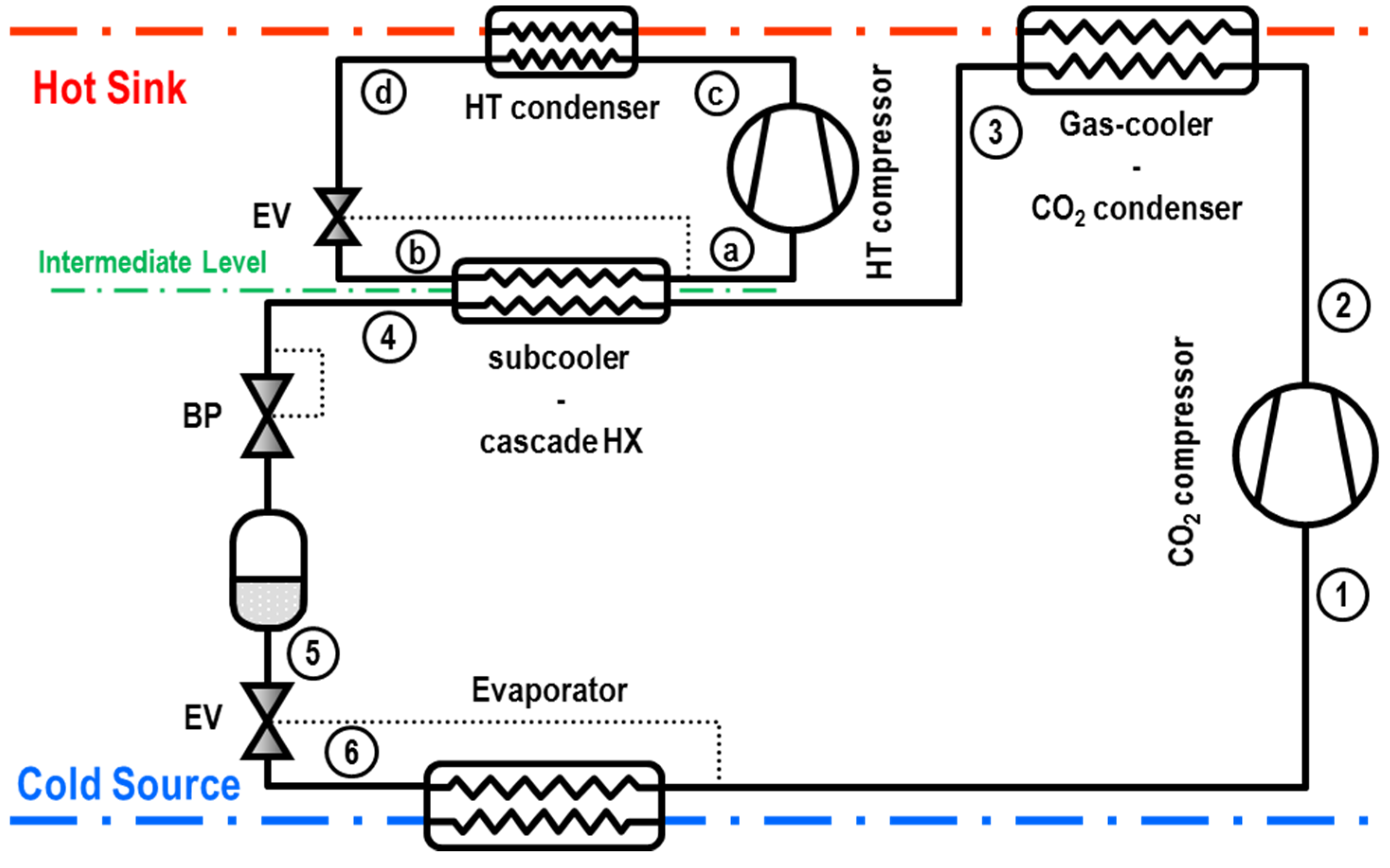
• A main cycle, working with CO₂ as refrigerant, which absorbs energy from the cold source.
• A CO₂ compressor, subcritical-rated for the cascade configuration and transcritical-rated for the MS configuration.
• A CO₂ gas-cooler, which performs heat rejection to the hot sink.
• A second CO₂ heat exchanger acting as CO₂ condenser for the cascade system and as CO₂ subcooler for the MS configuration.
• An expansion system: composed of the ‘vessel + expansion valve’ for the cascade configuration and of a ‘back-pressure + vessel + expansion valve’ for the MS cycle.
• An auxiliary single-stage refrigeration cycle: working with another refrigerant (HCs, HFOs, NH₃, HFCs) as high temperature cycle in the cascade configuration and as dedicated mechanical subcooling cycle for the MS configuration. The auxiliary system, whose refrigerant is not distributed to the cooling appliances, absorbs heat from the intermediate temperature level and performs heat rejection to the same hot sink as the main cycle. In the cascade configuration, the auxiliary cycle performs CO₂ condensation and in the MS it only subcools the CO₂ at the exit of the gas-cooler.

The operation of the cycle of Figure 1 as cascade or as MS cycle will depend on the hot sink temperature (T_H) and on the high-pressure fixed by the back-pressure valve (P_high), as detailed in the following subsections.

2.1. CO₂ Refrigeration Cycle with Mechanical Subcooling (MS Cycle)

Essentially, the CO₂ refrigeration cycle with mechanical subcooling corresponds to a main CO₂ single-stage cycle that uses an auxiliary cycle, with small capacity, to provide subcooling at the exit of the gas-cooler/condenser [17]. This cycle operates in subcritical or transcritical conditions depending on the heat rejection temperature (T_H) and on the high-pressure established by the back-pressure valve (P_high).

The transition from subcritical to transcritical conditions was investigated by Ge et al. [20], Shao et al. [21], Tsamos el at. [22] and Sanchez et al. [23] for standard CO₂ refrigeration cycles, however, no reference for the transition was found when the CO₂ cycle uses a mechanical subcooling system. For the analysis of the MS cycle, the transition from transcritical to subcritical was established in terms of the maximum COP value reached by each operating mode although this transition in real plants would be difficult. The considerations are the following:

If saturation pressure of CO₂ at T_H is lower than the pressure fixed by the back-pressure (P_high) and this last is lower than the critical pressure of CO₂ (73.773 bar), the optimum operation conditions will be in subcritical-mode with liquid subcooling. These boundary conditions are detailed by Equation (1), and the corresponding pressure-enthalpy diagram of CO₂ represented in Figure 2. In this type of operation, the first CO₂ heat exchanger acts as condenser (point 2 to 3) and the subcooler subcools liquid CO₂ (points 3 to 4). The case of partial condensation in the CO₂ heat exchanger (point 2 to 3*) is possible, but the best energy results are obtained for complete condensation.

$${\mathrm{P}}_{\mathrm{sat},{\mathrm{CO}}_2}\left({\mathrm{T}}_{\mathrm{H}}\right)<{\mathrm{P}}_{\mathrm{high}}\le {\mathrm{P}}_{\mathrm{crit},{\mathrm{CO}}_2}$$

(1)

$${\mathrm{P}}_{\mathrm{high}}>{\mathrm{P}}_{\mathrm{crit},{\mathrm{CO}}_2}$$

(2)

For pressures fixed by the back-pressure (P_high) higher than the critical pressure, Equation (2), the optimum operating conditions are in transcritical mode, as represented by Figure 3. For this mode of operation, the first CO₂ heat exchanger acts as gas-cooler (point 2 to 3) and the subcooler subcools gas or liquid depending on the high-pressure and T_H temperature (in red). The intermediate temperature (T_I) corresponds to the evaporating level of the high pressure cicle, in green, and is always lower than T_H.

2.2. Cascade Refrigeration Cycle

Cascade refrigeration cycle corresponds to the combination of two main refrigeration cycles, one cycle working with CO₂ in the low temperature level, which is condensed and maintained in subcritical, by another cycle that uses a refrigerant with good performance at high evaporation temperatures. In this case, both cycles are necessary, since the operation of the low temperature cycle depends on the operation of the high temperature cycle. In addition in this case, the high temperature cycle has similar or higher cooling capacity than the low temperature cycle.

Figure 4 represents the operation of the CO₂ cycle in a cascade system. This is the mode of operation if the condition established by Equation (3) or Equation (4) is satisfied. That is, when the pressure established by the back-pressure (if present) or by the thermal equilibrium of condensation (P_high) is lower than the CO₂ saturation pressure at T_H, Equation (3). As established in Equation (4), if T_H is higher than the critical temperature of CO₂, the high-pressure (P_high) must be lower than the critical one to satisfy the condition.

$${\mathrm{P}}_{\mathrm{high}}<{\mathrm{P}}_{\mathrm{sat},{\mathrm{CO}}_2}\left({\mathrm{T}}_{\mathrm{H}}\right){ \mathrm{if} \mathrm{T}}_{\mathrm{H}}\le {\mathrm{T}}_{\mathrm{crit},{\mathrm{CO}}_2,} \mathrm{OR}$$

(3)

$${\mathrm{P}}_{\mathrm{high}}<{\mathrm{P}}_{\mathrm{crit},{\mathrm{CO}}_2}{ \mathrm{if} \mathrm{T}}_{\mathrm{H}}>{\mathrm{T}}_{\mathrm{crit},{\mathrm{CO}}_2}$$

(4)

In the subcritical mode, the gas-cooler performs a small heat rejection to T_H and then the high-temperature cycle condenses CO₂ until saturated liquid. Subcooling is possible, but it offers worse results than the exit in saturation conditions because the intermediate temperature will need to descend.

This cycle was experimentally investigated by Dopazo et al. [24] using NH₃/CO₂ and Sanz et al. [12] using HFC134a/CO₂.

2.3. Calculation Models and Assumptions

We performed the analysis of the MS and the cascade cycles using simplified but realistic models, which assumptions are detailed then.

CO₂ compressor for both configurations is modeled using the overall efficiency as a linear relation with the compression ratio, as detailed by Equation (5). We fitted this relation using experimental data of a semi-hermetic single-stage CO₂ compressor able to operate in subcritical or transcritical [23].

$${\mathsf{\eta }}_{\mathrm{G},{\mathrm{CO}}_2}=0.7359-0.0517{\mathrm{t}}_{{\mathrm{CO}}_2}$$

(5)

For either the MS and cascade configurations, an approach temperature in gas-cooler of 5 K regards the environment temperature and 10 K of superheating degree in evaporator are chosen. For the MS configuration, when working in transcritical conditions, the high-pressure is established by the back-pressure. The tunable parameters are the high-pressure and the subcooling degree in subcooler (SUB = T₃ − T₄). Both parameters are optimized to obtain the best performing conditions. When working in subcritical, high pressure is computed as saturation temperature of CO₂ at the environment temperature plus a temperature difference in condenser of 5 K, to maintain the same reference level as in transcritical. The exit of the condenser is considered in saturation. Only the subcooling degree in the subcooler is free, it being optimized in the calculations. For the cascade configuration, the tunable variable is the temperature of the intermediate level, being the CO₂ condensing temperature taken as reference and optimized in the calculations. In this case, the exit condition of CO₂ of the cascade heat exchanger is considered in saturation. For both cycles, the lamination processes are assumed isenthalpic and pressure losses and heat transfer to the environment in the lines are neglected.

Regarding the secondary refrigerant, R1234yf is selected for the MS cycle and for the high-temperature cycle. This HFO is one of the new generation of refrigerants introduced to the market with the aim of substitute the R134, being an alternative with low GWP but light inflammable (A2L), that can perform as drop-in replacement. Aprea et al. [25] find out that this drop-in allows increasing the cooling capacity, being a refrigerant suitable for new plants and plants that are already working.

The overall efficiency of the compressor is also adjusted as a linear relation with the compression ratio, as detailed by Equation (6), in this case fitted from experimental data of a semi-hermetic compressor [26].

$${\mathsf{\eta }}_{\mathrm{G},\mathrm{R}1234\mathrm{yf}}=0.9721-0.0533{\mathrm{t}}_{\mathrm{R}1234\mathrm{yf}}$$

(6)

The high-temperature cycle or dedicated mechanical subcooling cycle, is thermally linked to the CO₂ cycle using two different approaches: when working as condenser in the cascade configuration, the evaporation temperature of R1234yf is considered to be 5 K below the CO₂ condensing temperature [12], thus being optimized during the calculation. On the other hand, when this cycle operates as mechanical subcooler, its evaporation temperature is computed considering a thermal effectiveness of the subcooler of 60%, Equation (7), being this effectiveness the average value measured in [27]. This temperature is indirectly optimized by tuning of the optimum subcooling degree in the CO₂ cycle.

$${\mathrm{T}}_{\mathrm{o},\mathrm{R}1234\mathrm{yf},\mathrm{MS}}={\mathrm{T}}_3-\frac{\mathrm{SUB}}{\mathsf{\epsilon }}={\mathrm{T}}_3-\frac{{\mathrm{T}}_3-{\mathrm{T}}_4}{\mathsf{\epsilon }}$$

(7)

For this cycle, a degree of superheat in the evaporator of 5 K is chosen. The exit of the condenser is in saturation and the expansion process is isenthalpic. Also, pressure losses and heat transfer to the environment in pipes are neglected.

The relation between the refrigerant mass flow rates of both cycles is obtained through the energy balance in the subcooler/cascade HX as established by Equation (8) according to nomenclature of Figure 1.

$$\frac{{\dot{\mathrm{m}}}_{\mathrm{R}1234\mathrm{yf}}}{{\dot{\mathrm{m}}}_{{\mathrm{CO}}_2}}=\frac{{\mathrm{h}}_3-{\mathrm{h}}_4}{{\mathrm{h}}_{\mathrm{a}}-{\mathrm{h}}_{\mathrm{b}}}$$

(8)

Using relation (8), the main energy parameters can be expressed as a function of the refrigerant enthalpies and the overall efficiencies of the compressors. Equation (9) expresses the overall COP of the cycle combination as quotient between the cooling capacity of the CO₂ cycle and the sum of power consumptions of both compressors. Equation (10) establishes the relation between the power consumption of the MS/cascade compressor regards the power consumption of the CO₂ compressor, it being an indicative of the size of the auxiliary cycle.

$$\mathrm{COP}=\frac{{\dot{\mathrm{Q}}}_{\mathrm{O}}}{{\mathrm{P}}_{\mathrm{C},{\mathrm{CO}}_2}+{\mathrm{P}}_{\mathrm{C},\mathrm{R}1234\mathrm{yf}}}=\frac{{\mathrm{h}}_1-{\mathrm{h}}_4}{\frac{{\mathrm{h}}_{2,\mathrm{s}}-{\mathrm{h}}_1}{{\mathsf{\eta }}_{\mathrm{G},{\mathrm{CO}}_2}}+\frac{{\mathrm{h}}_3-{\mathrm{h}}_4}{{\mathrm{h}}_{\mathrm{a}}-{\mathrm{h}}_{\mathrm{b}}}\times \frac{{\mathrm{h}}_{\mathrm{c},\mathrm{s}}-{\mathrm{h}}_{\mathrm{a}}}{{\mathsf{\eta }}_{\mathrm{G},\mathrm{R}1234\mathrm{yf}}}}$$

(9)

$$\frac{{\mathrm{P}}_{\mathrm{C},\mathrm{R}1234\mathrm{yf}}}{{\mathrm{P}}_{\mathrm{C},{\mathrm{CO}}_2}}=\frac{\left({\mathrm{h}}_3-{\mathrm{h}}_4\right)\times \left({\mathrm{h}}_{\mathrm{c},\mathrm{s}}-{\mathrm{h}}_{\mathrm{a}}\right)}{\left({\mathrm{h}}_{\mathrm{a}}-{\mathrm{h}}_{\mathrm{b}}\right)\times \left({\mathrm{h}}_{2,\mathrm{s}}-{\mathrm{h}}_1\right)}\times \frac{{\mathsf{\eta }}_{\mathrm{G},{\mathrm{CO}}_2}}{{\mathsf{\eta }}_{\mathrm{G},\mathrm{R}1234\mathrm{yf}}}$$

(10)

All the thermophysical properties of the refrigerants have been calculated using Refprop database [28].

3. Results

This section establishes the optimum operating conditions of the CO₂ refrigeration cycle with mechanical subcooling (Section 3.1) and of the cascade cycle using CO₂ as low temperature fluid (Section 3.2) using the model detailed in Section 2. The evaluation was made considering environment temperatures from 15 to 40 °C and evaporating levels from 5 to −20 °C. No lower evaporating levels were analyzed because −20 °C corresponds to the lowest evaporating temperature at which the CO₂ compressor used to build the correlations can be operated. For lower evaporating levels, two stage solutions should be considered.

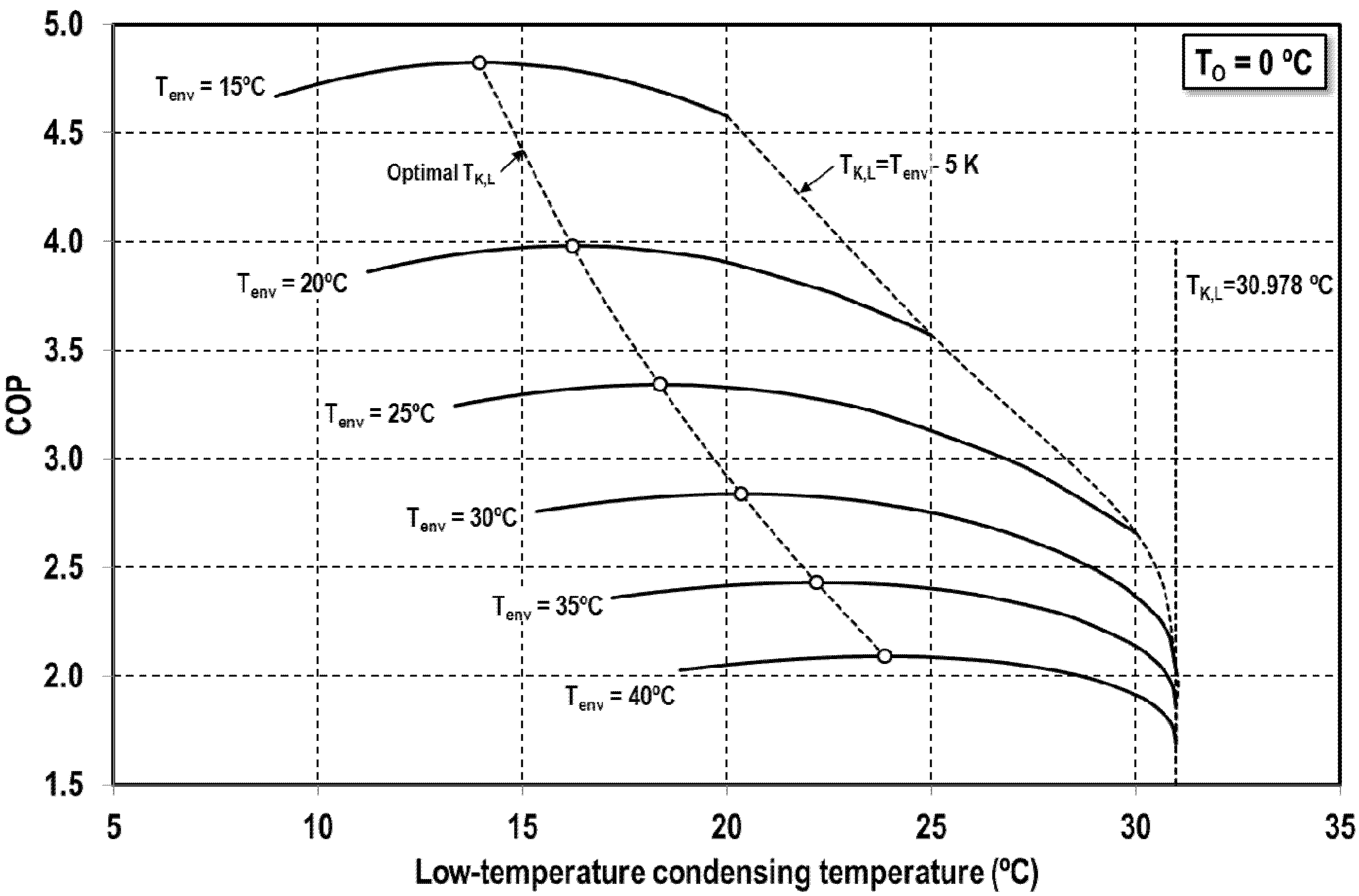
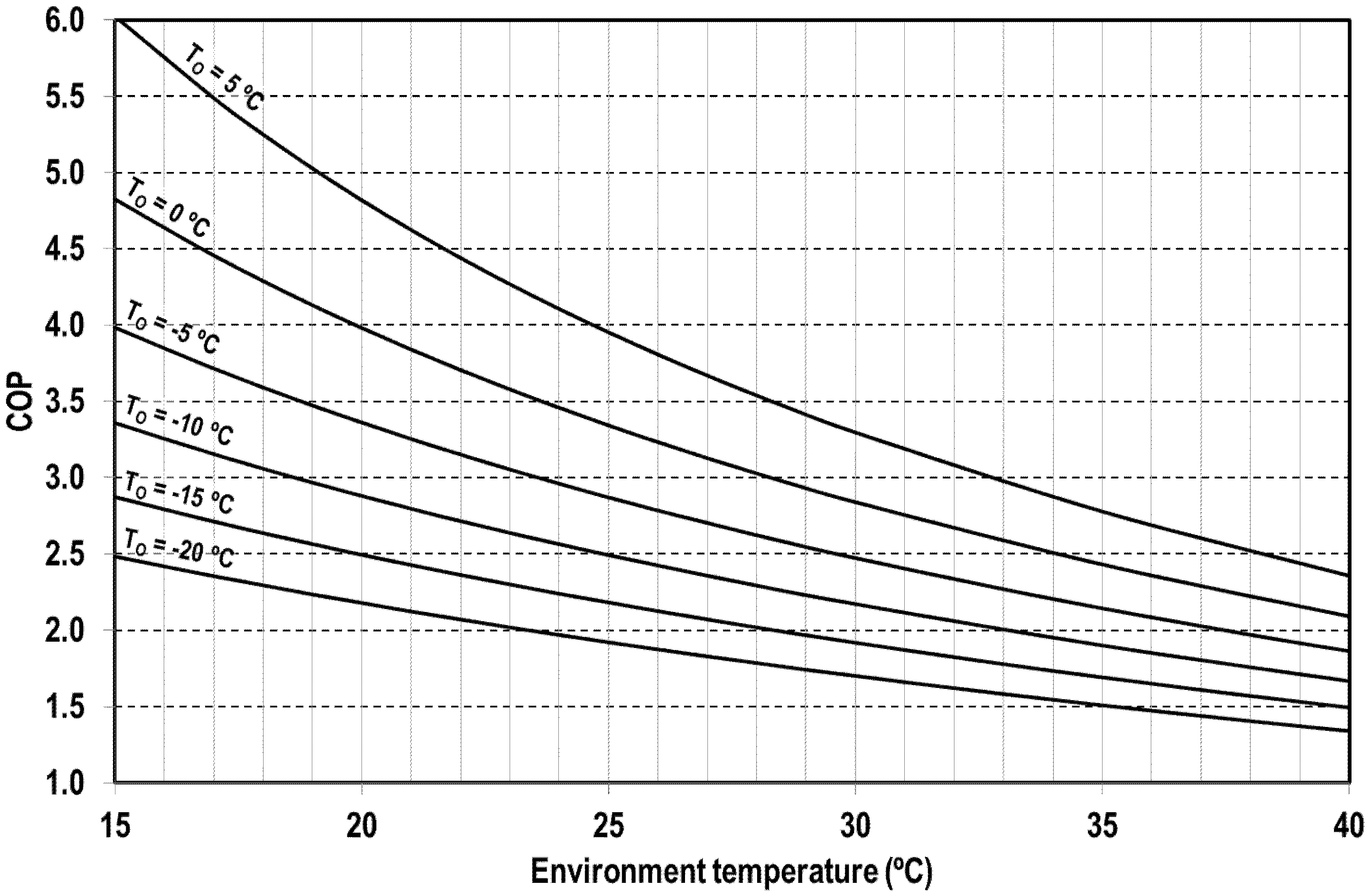
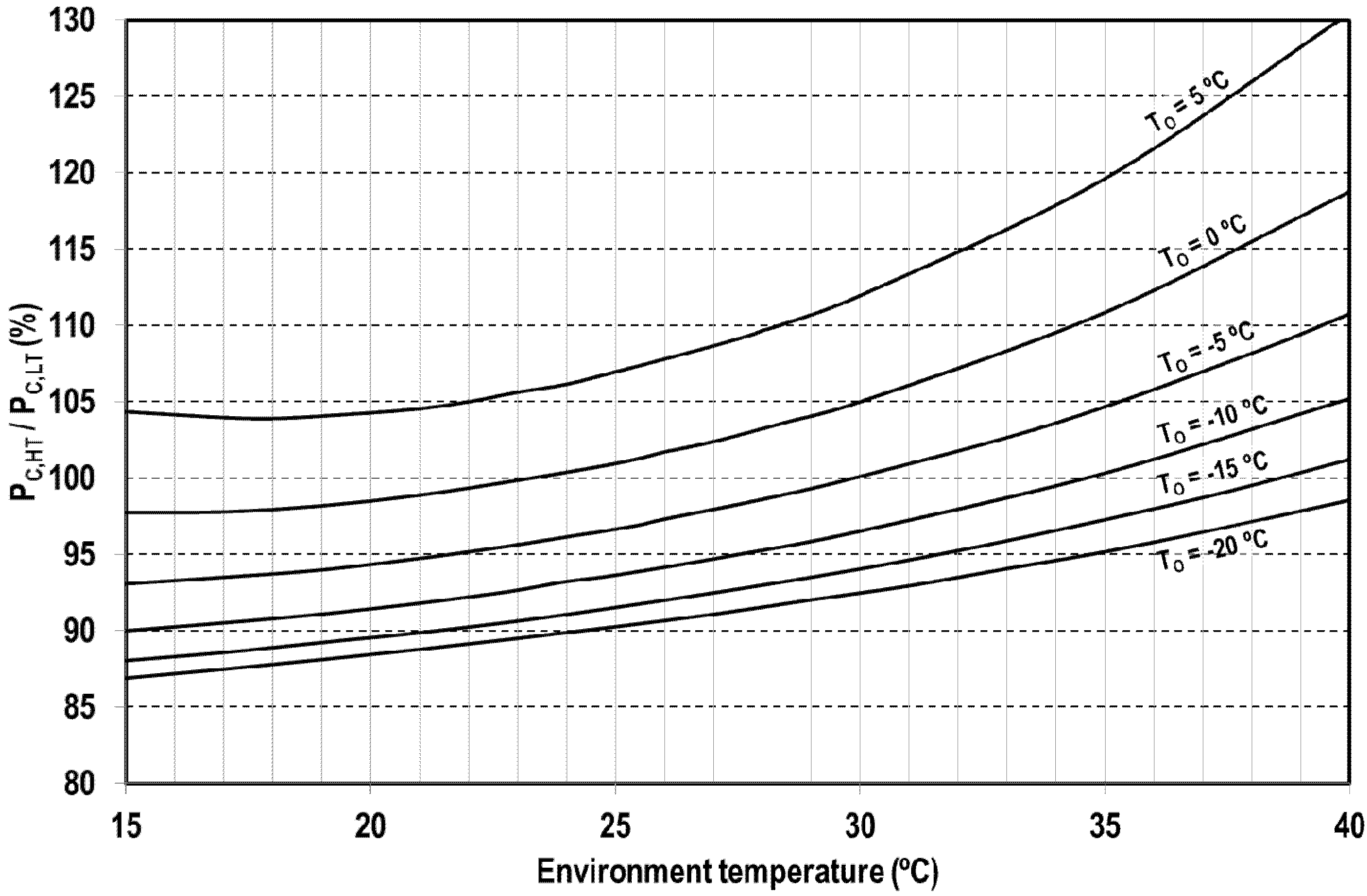
3.1. Operating Conditions of the CO₂ Cycle with Mechanical Subcooling

As mentioned, the operating parameters to be tuned to obtain the best performing conditions of the CO₂ cycle with mechanical subcooling are the pressure at the gas-cooler (P_high) and the degree of subcooling provided by the auxiliary system (SUB). To illustrate the behavior of this cycle, the dependence of the overall COP, Equation (9), versus the environment temperature and the subcooling degree for an evaporating level of 0 °C is presented in Figure 5. Data of Figure 5 are evaluated for the optimum gas-cooler pressures. For environment temperatures below 25 °C the best results are in subcritical operation and for warmer temperatures in transcritical. As it can be observed, for any environment temperature, an optimum degree of subcooling exists, maximizing the overall COP. Furthermore, it is observed that the subcooling degree increases when going to warmer temperatures.

Maximum COP for the considered range and the corresponding optimum subcooling degrees are detailed in Figure 6 and Figure 7, respectively, for all the considered range. As it can be observed in Figure 6, the transition between subcritical to transcritical operation occurs, from a theoretical energy point of view, at an environment temperature of 25.3 ± 0.2 °C. Since this temperature is commonly reached in any location, the plant must be designed to be able to operate in subcritical conditions when possible, since forcing it to operate in transcritical would result in reductions of COP. That means that the first CO₂ heat exchanger must be sized as condenser, but it must be ready to operate also as gas-cooler. The trend is the same as in pure CO₂ transcritical systems, as it can be observed in the work presented by Sanchez D. et al. [23]. Another important aspect is that the presence of the optimum subcooling degree disappears when temperature difference between T_C and T_H is high. It can be observed for the operation at −5 °C and below. It will be mentioned later, but the reason is that at a high temperature lift the MS cycle is overcome by the cascade solution.

Finally, the ratio between the power consumption of the auxiliary cycle (R1234yf) and the main compressor (CO₂), Equation (10), are represented in percentage for the optimum operating conditions in Figure 8. For the considered range, the needed power consumption of the auxiliary compressor ranges from 4% at an evaporation of 5 °C and environment temperature of 15 °C to 21% approximately for 5 °C at 40 °C. The most important observation is that sizing the auxiliary compressor for high environment temperatures will cover the operation in transcritical and subcritical without problems.

3.2. Operating Conditions of the Cascade Cycle

For the cascade cycle, the parameter that must be optimized is the intermediate temperature level (T_I), the condensing temperature of CO₂ (T_K,L) being considered in this case for its representation. As mentioned, exit of CO₂ cascade condenser is in saturation, no subcooling is considered, because it provides lower efficiency results. Figure 9 presents the evolution of the overall COP of the cascade solution for an evaporation level of 0 °C for all the considered environment temperatures. Limits of variation of T_K,L are any temperature over the evaporating pressure up to a condensing temperature 5 K below the environment temperature (if T_env < 25.978 °C) or the critical temperature. In Figure 9 it becomes clear that an optimum T_K,L temperature exists. No more emphasis is done because different authors studied it in detail [29,30]. COP values at the optimum T_K,L are presented in Figure 10. In contrast to the COP evolutions of the MS cycle, it needs to be highlighted that the reduction of COP of cascade systems due to variations of the environment temperature is smoother, being these systems less sensitive to variations of environmental conditions, as previously mentioned by Llopis et al. [14]. Also, to compare the design of the cascade system, the ratio of the high-temperature and low-temperature power consumption are presented in Figure 11. In this case, the power consumption of the high-temperature compressor inside the evaluated range is of the same order of magnitude as that of the CO₂ cycle. With a design of the plant as cascade, it could operate with the MS cycle but not the other way round.

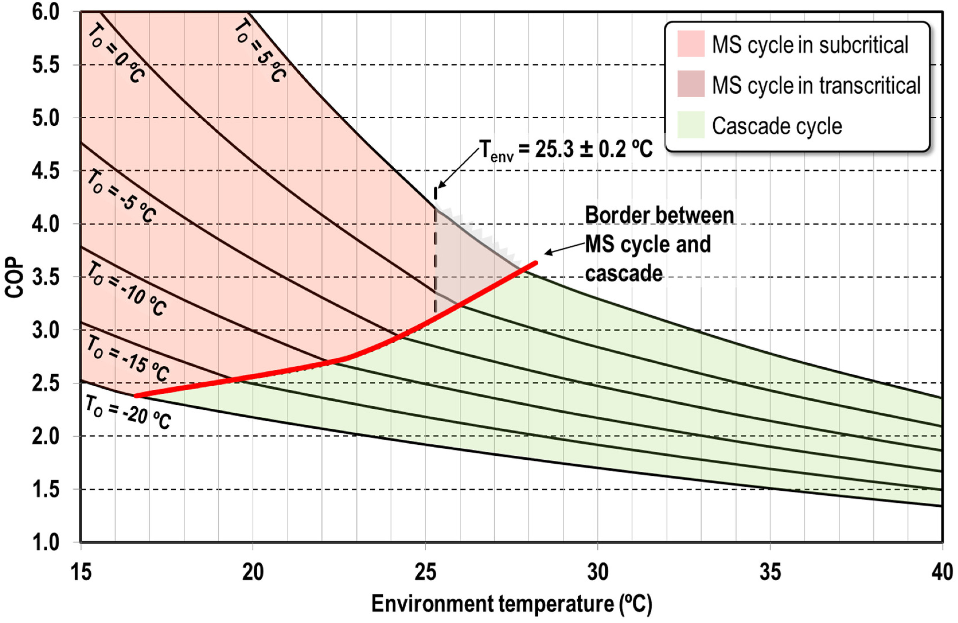
4. Discussion of Results

The optimum operating conditions of both cycles were analyzed in Section 3. As mentioned, both refrigeration cycles respond to the same scheme of operation (Figure 1) and may be able to operate with one scheme or the other if some components of the plant are over-sized. However, in practice, only one design of the plant is implemented due to economic reasons, for example: if the plant is designed to be operated in both modes the cascade/subcooler heat exchanger must be sized as cascade heat exchanger, while if it were designed to be operated as MS cycle the subcooler would be size reduced. The same happens for the gas-cooler, a gas-cooler of a cascade system is smaller than that of the MS cycle. Furthermore, if optimum COP results of both solutions are compared (Figure 6 and Figure 10) it can be seen that the MS cycle offers the best results at low environment temperatures and the cascade at high temperatures. Thus, this section is devoted to compare the COP values offered by both solutions. First, the recommended operating range of each cycle is analyzed in terms of COP, and then the results are translated to the different climatic regions of Spain through the computation of the average annual COP. The objective is to obtain conclusions about which system would be more recommended for a given evaporating level in a given climatic region.

4.1. Recommended Operating Conditions

COP values offered by both cycle configurations are merged in Figure 12, where the COP value at each evaporating and environment level corresponds to the best performing system. As it can be observed, the cascade system gets over the MS solution at high environment temperatures and low evaporating levels. In fact, the environment temperature for a given evaporating level that defines the border of both systems is expressed by Equation (11), which was fitted from the results of the models. At environment temperatures above the value given by Equation (11), the cascade solution operates with highest COP. Also, the optimum modes of operation of the MS cycle are depicted in Figure 12. The operating conditions between an environment temperature of 25.3 °C and that defined by Equation (11) will be in transcritical conditions, whereas all lower environment levels the best performing cycle will be in subcritical. As it is observed in Figure 12, the environmental conditions at which the plant would be operated in transcritical are very narrow, which means that the correct design of the first CO₂ heat exchanger would be as condenser. In an attempt to summarize all the results of Figure 12, the COP dependence of both cycles versus the temperature difference between the cold and hot sources, Equation (12), is presented in Figure 13. Data used in Figure 13 correspond to all the calculated points to represent Figure 12. It can be observed that the MS cycle offers highest COP values at reduced temperature lifts and the cascade the other way round. The limit is at a temperature lift of 28.5 K approximately. However, it is important to note that the difference between the COP values of the MS cycle regards the cascade are higher at low temperature lifts that the difference between them at high temperature lifts. Those COP differences will condition the operation of the system along different environment temperatures, therefore a climatic evaluation would be needed to compare both cycles. That is discussed in Section 4.2.

$${\mathrm{T}}_{\mathrm{env}}=25.95+0.4{\mathrm{T}}_{\mathrm{o}}$$

(11)

$$∆\mathrm{T}={\mathrm{T}}_{\mathrm{env}}-{\mathrm{T}}_{\mathrm{o}}$$

(12)

Although in Figure 12 it seems that a smooth transition between the MS and the cascade cycle would be possible, it will only happen when the cycle is sized to operate in both configurations. To illustrate this reasoning, the compressor’s displacements for the low and high temperature cycles for both configurations are presented in Figure 14. Those data correspond to the displacements for a refrigeration plant with 50 kW of cooling capacity designed for an environment temperature of 30 °C. It can be observed that the differences of the CO₂ compressor are not much significant between both cycles’ solutions, but the compressor of the cascade cycle would be up to 300% higher than that needed for the MS cycle. If the plant is sized to be operated as MS cycle, its operation as cascade would not be possible because of the compressors, and, although not evaluated, because of the size of the subcooler and the gas-cooler.

4.2. Operation in Different Climate Conditions

As mentioned by Minetto et al. [31], the superiority of one refrigeration system regards another in terms of energy efficiency must be discussed with reference to the climatic conditions of the installation site and the characteristics of cooling profile. In agreement with them, and in order to obtain conclusions about the performance of the MS cycle configuration regards the cascade design, in this subsection an evaluation of the systems at different climate conditions is reported. In this case, a climatic evaluation was made using the BIN temperature methodology [32] with the Energy Plus meteorological data (https://energyplus.net/weather) for different locations in Spain. This methodology groups the number of annual hours in which a certain temperature was recorded, allowing an accurate representation of the annual climate.

In fact, the energy performance of the systems was evaluated for the twelve climatic regions of Spain [33],

Table 1. Reference Spanish cities for the evaluation of the systems. Climatic regions, temperature BINs, hours of operation and cooling load profiles.

City			León	Pamplona	Teruel	Albacete	La Coruña	Barcelona	Granada	Toledo	Castellón de la Plana	Sevilla	Málaga	Almería
Spanish climatic region			E1	D1	D2	D3	C1	C2	C3	C4	B3	B4	A3	A4
Average annual temperature (°C)			10.79	12.22	11.55	13.51	14.14	15.37	14.88	15.57	16.74	18.25	17.99	18.54
Temperature BIN	AC cooling load (%)	Commercial cooling load (%)	Annual hours inside the temperature BIN
<−3	0	0.5	0	0	0	0	0	0	0	0	0	0	0	0
−3 to −1	0	0.5	0	0	0	0	0	0	0	0	0	0	0	0
−1 to 1	0	0.5	248	0	391	0	0	0	0	0	0	0	0	0
1 to 3	0	0.5	990	341	878	633	0	0	248	155	0	0	0	0
3 to 5	0	0.5	936	962	875	847	0	0	692	602	0	0	0	0
5 to 7	0	0.5	847	1114	633	817	0	540	843	663	124	62	0	0
7 to 9	0	0.5	915	819	887	571	537	909	571	876	903	754	62	0
9 to 11	0	0.5	818	884	734	981	1697	1057	827	663	968	846	996	810
11 to 13	0	0.5	943	846	751	604	1364	819	668	949	813	785	1055	943
13 to 15	0	0.5	826	944	855	756	1553	1063	851	572	854	789	941	933
15 to 17	0	0.5	552	765	733	669	1556	824	814	638	943	858	884	975
17 to 19	0	0.5	492	615	522	705	950	817	795	578	909	841	1061	1094
19 to 21	0	0.5	244	430	430	583	673	1046	612	764	976	1008	1002	851
21 to 23	0.2	0.5	304	274	213	339	430	613	307	615	800	581	919	1068
23 to 25	0.4	0.6	304	304	244	306	0	518	461	431	552	581	738	800
25 to 27	0.6	0.7	155	276	273	273	0	337	214	275	394	523	397	488
27 to 29	0.8	0.8	186	186	217	304	0	217	243	183	338	275	426	458
29 to 31	1	0.9	0	0	124	124	0	0	273	393	186	243	279	340
31 to 33	1	1	0	0	0	217	0	0	124	155	0	304	0	0
>33	1	1	0	0	0	31	0	0	217	248	0	310	0	0

, covering cold, mild and warm climates, using 20 temperature BINs from −3 to 33 °C of dry bulb temperature. For the evaluation, two simplified cooling load profiles were considered. Representing air-conditioning (AC) applications, no cooling load was considered below 21 °C, a linear dependence on the cooling load from temperatures above 21 up to 29 °C and 100% from 29 °C on. For commercial applications a constant value of 50% of cooling load up to 23 °C, linear dependence from 23 to 31 °C and 100% from 31 ºC on. Cooling load profiles are detailed in Table 1.

Using the meteorological data of dry-bulb temperature, an averaged COP value for both cycle configurations was evaluated using Equation (13). Where COP (T_env,i) is the COP of each system evaluated at the average temperature of the ‘i’ temperature BIN, NH_i is the number of hours of operation inside the ‘i’ temperature BIN and FQ_i the cooling load fraction inside the ‘i’ temperature BIN.

$$\overline{\mathrm{COP}}=\frac{{{\displaystyle \sum }}_{\mathrm{i}=1}^{\mathrm{nbin}}\left[\mathrm{COP}\left({\mathrm{T}}_{\mathrm{env},\mathrm{i}}\right)\times {\mathrm{NH}}_{\mathrm{i}}\times {\mathrm{FQ}}_{\mathrm{i}}\right]}{{{\displaystyle \sum }}_{\mathrm{i}=1}^{\mathrm{nbin}}\left({\mathrm{NH}}_{\mathrm{i}}\times {\mathrm{FQ}}_{\mathrm{i}}\right)}$$

(13)

Averaged COP values for both refrigeration systems, for the different climatic regions using the cooling load profiles detailed in Table 1, are summarized in

Table 2. Averaged annual COP of cascade and MS cycles for Spanish Climate Regions.

Climatic Region	E1	D1	D2	D3	C1	C2	C3	C4	B3	B4	A3	A4
Cascade cycle annual averaged COP
To = 5 °C (AC)	3.74	3.72	3.57	3.41	4.30	3.79	3.33	3.33	3.66	3.34	3.63	3.63
To = 0 °C	4.51	4.45	4.42	4.23	4.53	4.26	4.13	4.04	4.11	3.87	4.00	3.94
To = −5 °C	3.75	3.70	3.68	3.54	3.77	3.56	3.46	3.39	3.45	3.26	3.37	3.32
To = −10 °C	3.18	3.14	3.12	3.01	3.19	3.03	2.95	2.90	2.95	2.80	2.88	2.84
To = −15 °C	2.73	2.70	2.69	2.60	2.74	2.61	2.55	2.51	2.54	2.42	2.49	2.46
To = −20 °C	2.37	2.35	2.33	2.26	2.38	2.27	2.22	2.18	2.22	2.12	2.17	2.15
MS cycle annual averaged COP
To = 5 °C (AC)	3.92	3.88	3.65	3.43	4.82	4.00	3.32	3.33	3.80	3.34	3.76	3.76
To = 0 °C	5.65	5.52	5.48	5.14	5.67	5.16	4.97	4.81	4.89	4.49	4.68	4.56
To = −5 °C	4.38	4.29	4.26	4.02	4.40	4.04	3.89	3.78	3.85	3.55	3.70	3.62
To = −10 °C	3.50	3.44	3.41	3.23	3.52	3.25	3.14	3.06	3.11	2.89	3.00	2.94
To = −15 °C	2.86	2.81	2.79	2.65	2.87	2.67	2.58	2.51	2.56	2.38	2.48	2.43
To = −20 °C	2.36	2.32	2.30	2.19	2.37	2.21	2.13	2.08	2.12	1.98	2.06	2.02
Climatic region	E1	D1	D2	D3	C1	C2	C3	C4	B3	B4	A3	A4
Cascade cycle annual averaged COP
To = 5 °C (AC)	3.74	3.72	3.57	3.41	4.30	3.79	3.33	3.33	3.66	3.34	3.63	3.63
To = 0 °C	4.51	4.45	4.42	4.23	4.53	4.26	4.13	4.04	4.11	3.87	4.00	3.94
To = −5 °C	3.75	3.70	3.68	3.54	3.77	3.56	3.46	3.39	3.45	3.26	3.37	3.32
To = −10 °C	3.18	3.14	3.12	3.01	3.19	3.03	2.95	2.90	2.95	2.80	2.88	2.84
To = −15 °C	2.73	2.70	2.69	2.60	2.74	2.61	2.55	2.51	2.54	2.42	2.49	2.46
To = −20 °C	2.37	2.35	2.33	2.26	2.38	2.27	2.22	2.18	2.22	2.12	2.17	2.15
MS cycle annual averaged COP
To = 5 °C (AC)	3.92	3.88	3.65	3.43	4.82	4.00	3.32	3.33	3.80	3.34	3.76	3.76
To = 0 °C	5.65	5.52	5.48	5.14	5.67	5.16	4.97	4.81	4.89	4.49	4.68	4.56
To = −5 °C	4.38	4.29	4.26	4.02	4.40	4.04	3.89	3.78	3.85	3.55	3.70	3.62
To = −10 °C	3.50	3.44	3.41	3.23	3.52	3.25	3.14	3.06	3.11	2.89	3.00	2.94
To = −15 °C	2.86	2.81	2.79	2.65	2.87	2.67	2.58	2.51	2.56	2.38	2.48	2.43
To = −20 °C	2.36	2.32	2.30	2.19	2.37	2.21	2.13	2.08	2.12	1.98	2.06	2.02

. Regarding AC application (T_o = 5 °C), it can be seen that the MS cycle over performs the cascade configuration for all the climatic regions except for the D3, C3, C4 and B4, that are regions with high environment temperatures during summer, where both configuration perform similar. Regarding the general application, for evaporating temperatures from 0 to −20 °C, the MS cycle also presents highest performance for all the climatic regions up to an evaporating level of −10 °C. At −15 °C both solutions perform similar and for −20 °C the cascade solution is the best performing. The differences between both refrigeration systems for the different climate conditions and the different evaporating levels and cooling load profiles are represented in Figure 15 as percentage variation from the MS cycle COP values, according to Equation (14). Values of Equation (14) represent the average annual COP advantage of the MS cycle regard the cascade cycle. It can be observed that the MS cycle is recommended from an energy point of view for any evaporating level higher or equal to −10 °C, both systems similar perform at −15 °C and the cascade should be recommended for the temperature level of −20 °C.

$$∆\mathrm{COP} (\%)=\frac{{\mathrm{COP}}_{\mathrm{MS}}-{\mathrm{COP}}_{\mathrm{casc}}}{{\mathrm{COP}}_{\mathrm{casc}}}\times 100$$

(14)

As previously mentioned, both refrigeration cycle designs could be implemented in a system if some of the components are oversized, mainly the high temperature compressor, subcooler and gas-cooler/condenser, although it is not commonly done. Nonetheless, if only one cycle of operation is selected, it is important to quantify what would be its overall performance regards a plant with possibility to operate as cascade or as MS cycle, that would be the plant that will offer the best average annual COP values. To quantify the differences of the individual systems, their average annual COP values according to Equation (13) were compared to the ones obtained by an ideal refrigeration system with COP values equal to the maximum COP values of the MS or the cascade system. Percentage annual COP deviations regards the ideal system are specified in

Table 3. Percentage deviation of annual COP values of MS and cascade cycles regards the best system.

Climatic Region	E1	D1	D2	D3	C1	C2	C3	C4	B3	B4	A3	A4
Cascade cycle
To = 5 °C (AC)	−4.7	−4.3	−3.1	−2.6	−10.9	−5.2	−2.5	−2.8	−4.3	−2.7	−4.2	−4.1
To = 0 °C	−20.2	−19.6	−19.6	−18.2	−20.0	−17.5	−17.4	−16.6	−16.2	−14.6	−14.9	−14.2
To = −5 °C	−14.6	−14.1	−14.1	−12.9	−14.3	−12.3	−12.3	−11.6	−11.2	−10.0	−10.1	−9.5
To = −10 °C	−9.7	−9.3	−9.3	−8.4	−9.3	−7.8	−7.9	−7.4	−6.9	−6.1	−6.2	−5.7
To = −15 °C	−5.5	−5.2	−5.2	−4.6	−5.0	−4.1	−4.2	−4.0	−3.6	−3.1	−3.1	−2.8
To = −20 °C	−1.4	−1.3	−1.3	−1.1	−1.1	−1.0	−1.0	−1.0	−0.8	−0.7	−0.7	−0.6
MS cycle
To = 5 °C (AC)	−0.2	−0.2	−0.8	−2.0	0.0	−0.1	−2.7	−2.8	−0.7	−2.7	−0.8	−0.8
To = 0 °C	−0.1	−0.1	−0.2	−0.5	0.0	−0.1	−0.7	−0.9	−0.4	−1.1	−0.5	−0.6
To = −5 °C	−0.3	−0.3	−0.5	−1.0	0.0	−0.5	−1.3	−1.5	−0.8	−1.9	−1.1	−1.3
To = −10 °C	−0.6	−0.7	−0.9	−1.6	−0.1	−1.0	−2.0	−2.4	−1.6	−3.1	−2.1	−2.4
To = −15 °C	−1.1	−1.3	−1.5	−2.5	−0.4	−2.0	−3.1	−3.7	−2.9	−4.7	−3.6	−4.1
To = −20 °C	−1.9	−2.4	−2.6	−4.0	−1.5	−3.8	−4.8	−5.6	−5.0	−7.1	−6.1	−6.7

for the different Spanish climate regions, and represented for two representative cases in Figure 16, which correspond to the operation at −5 °C and −20 °C of evaporating temperature. As it can be observed, any individual system has reductions of annual COP values regards the optimum or best system, since in some hours of the year the other solution would be more performing. That occurs for all the climatic regions and evaporating levels except for the climatic region C1 with evaporating levels from 5 to −5 °C. In general, for all the climatic regions, the system that better performs is the MS cycle configuration, with annual deviations from the best system up to 5% at evaporating levels higher or equal than −15 °C. On the other side, if the considered evaporating level is −20 °C, the solution with less deviation from the ideal system is the cascade, however, it is important to note that the MS cycle will have deviations lower than 5% regards the ideal system for all the climatic regions except for the C4, B4, A3 and A4. That indicates that although the MS cycle does not reach the performance of the cascade solution at −20 °C, its average annual performance would be good enough for all the climatic conditions without large reductions of efficiency. This solution will avoid the over sizing of the plant, and thus, allow to operate with a lower cost plant.

5. Conclusions

This communication analyzes two modes of operation of a CO₂-based two-stage refrigeration cycle with equivalent design that can be operated as cascade refrigeration system or as a CO₂ refrigeration plant with dedicated mechanical subcooling system. Both schemes are being considered now to spread the use of CO₂ in medium and warm regions of the planet for medium temperature applications.

Using relations of the overall efficiency of compressors, adjusted from experimental data of a semi-hermetic CO₂ and a semi-hermetic R1234yf compressors, a simplified model of both cycles was developed. With the thermodynamic models, the optimum operating conditions of each refrigeration cycle, covering evaporating temperatures from −20 to 5 °C and environment temperatures from 15 to 40 °C, were determined. Then, by merging the COP values of each refrigeration solution, the external conditions at which each refrigeration solution is the best performing were established. Furthermore, the analysis was translated for the different climatic regions of Spain to compare the systems.

Regarding the CO₂ refrigeration cycle with mechanical subcooling, it was concluded that the environment temperature that will limit the operation in subcritical or transcritical is 25.3 °C, thus the design of the gas-cooler would be always as condenser, since the region at which this system will operate in transcritical is very narrow. Furthermore, the optimum subcooling degree results higher at lowest evaporating levels and high environment levels. Nonetheless, the maximum ratio of power consumption of the mechanical subcooling compressor will not exceed from 21% of the power consumption of the CO₂ compressor.

It was concluded that the cascade configuration using CO₂ as low temperature refrigerant will have highest performance than the MS cycle when the temperature lift between the cold and heat sources is higher than 28.5 K. However, in this case the power consumption of the high-temperature cycle will be even higher than the power consumption of the CO₂ rack.

The analysis was extended to the different climatic regions of Spain using a based temperature-BIN methodology. It was calculated that the MS cycle would offer highest energy efficiencies in overall-year operation than the cascade solution for evaporating levels below −15 °C, including the air-conditioning application. However, at the evaporating level of −20 °C the cascade solution will over perform the MS cycle. Also, the individual systems were compared to an ideal refrigeration cycle that could be operated as CO₂ with mechanical subcooling or as cascade at any climatic condition, which is called the best system. The average annual COP of each individual system was compared with the best system. It was observed that the MS cycle will have annual reductions of efficiency up to 5% at evaporating levels higher or equal than −15 °C, and also reductions below 5% at the evaporating level of −20 °C except for 4 climatic regions of Spain.

As general conclusion of this work, it can be affirmed that if this cycle configuration is sized as cascade or as a single-stage cycle with mechanical subcooling, the configuration that will offer the best performing levels at the analyzed conditions would be the CO₂ refrigeration cycle with mechanical subcooling.

References and Notes

1. European Commission. Regulation (EU) No 517/2014 of the European Parliament and of the Council of 16 April 2014 on Fluorinated Greenhouse Gases and Repealing Regulation (EC) No 842/2006, 2014.
2. Hafner, A.; Hemmingsen, A.K. R744 refrigeration technologies for supermarkets in warm climates. In Proceedings of the 24th IIR International Congress of Refrigeration, Yokohama, Japan, 16–22 August 2015. [Google Scholar]
3. Kim, M.H.; Pettersen, J.; Bullard, C.W. Fundamental process and system design issues in CO2 vapor compression systems. Prog. Energy Combust. Sci. 2004, 30, 119–174. [Google Scholar] [CrossRef]
4. Jia, X.; Zhang, B.; Pu, L.; Guo, B.; Peng, X. Improved rotary vane expander for trans-critical CO2 cycle by introducing high-pressure gas into the vane slots. Int. J. Refrig. 2011, 34, 732–741. [Google Scholar] [CrossRef]
5. Hu, J.; Li, M.; Zhao, L.; Xia, B.; Ma, L. Improvement and experimental research of CO2 two-rolling piston expander. Energy 2015, 93, 2199–2207. [Google Scholar] [CrossRef]
6. Elbel, S.; Lawrence, N. Review of recent developments in advanced ejector technology. Int. J. Refrig. 2016, 62, 1–18. [Google Scholar] [CrossRef]
7. Hafner, A.; Banasiak, K.; Herdlitschka, T.; Fredslund, K.; Girotto, S.; Haida, M.; Smolka, J. ‘R744 Ejector System Case: Italian Supermarket, Spiazzo’, in Refrigeration Science and Technology. 2016; 471–478. [Google Scholar]
8. Lawrence, N.; Elbel, S. ‘Experimental Study on Control Methods for Transcritical Co2 Two-Phase Ejector Systems at Off-Design Conditions’, in Refrigeration Science and Technology. 2016; 511–518. [Google Scholar]
9. Karampour, M.; Sawalha, S. ‘Integration of Heating and Air Conditioning into a Co2 Trans-Critical Booster System with Parallel Compression Part I: Evaluation of Key Operating Parameters Using Field Measurements’, in Refrigeration Science and Technology. 2016; 323–331. [Google Scholar]
10. Aprea, C.; Greco, A.; Maiorino, A. The application of a desiccant wheel to increase the energetic performances of a transcritical cycle. Energy Convers. Manag. 2015, 89, 222–230. [Google Scholar] [CrossRef]
11. Arora, A.; Singh, N.K.; Monga, S.; Kumar, O. Energy and exergy analysis of a combined transcritical CO2 compression refrigeration and single effect H2O-LiBr vapour absorption system. Int. J. Exergy 2011, 9, 453–471. [Google Scholar] [CrossRef]
12. Sanz-Kock, C.; Llopis, R.; Sánchez, D.; Cabello, R.; Torrella, E. Experimental evaluation of a R134a/CO2 cascade refrigeration plant. Appl. Therm. Eng. 2014, 73, 39–48. [Google Scholar] [CrossRef]
13. Peñarrocha, I.; Llopis, R.; Tárrega, L.; Sánchez, D.; Cabello, R. A new approach to optimize the energy efficiency of CO2 transcritical refrigeration plants. Appl. Therm. Eng. 2014, 67, 137–146. [Google Scholar] [CrossRef]
14. Llopis, R.; Sánchez, D.; Sanz-Kock, C.; Cabello, R.; Torrella, E. Energy and environmental comparison of two-stage solutions for commercial refrigeration at low temperature: Fluids and systems. Appl. Energy 2015, 138, 133–142. [Google Scholar] [CrossRef]
15. Hafner, A.; Hemmingsen, A.K.; Van De Ven, A. ‘R744 Refrigeration System Configurations for Supermarkets in Warm Climates’, in Refrigeration Science and Technology. 2014; 125–133. [Google Scholar]
16. Gullo, P.; Elmegaard, B.; Cortella, G. Energy and environmental performance assessment of R744 booster supermarket refrigeration systems operating in warm climates. Int. J. Refrig. 2016, 64, 61–79. [Google Scholar] [CrossRef] [Green Version]
17. Llopis, R.; Cabello, R.; Sánchez, D.; Torrella, E. Energy improvements of CO2 transcritical refrigeration cycles using dedicated mechanical subcooling. Int. J. Refrig. 2015, 55, 129–141. [Google Scholar] [CrossRef]
18. Nebot-Andrés, L.; Llopis, R.; Sánchez, D.; Cabello, R. Experimental evaluation of a dedicated mechanical subcooling system in a CO2 transcritical refrigeration cycle, Refrigeration Science and Technology. 2016; 965–972. [Google Scholar]
19. Eikevik, T.M.; Bertelsen, S.; Haugsdal, S.; Tolstorebrov, I.; Jensen, S. ‘Co2 Refrigeration System with Integrated Propan Subcooler for Supermarkets in Warm Climate’, in Refrigeration Science and Technology. 2016; 211–218. [Google Scholar]
20. Ge, Y.T.; Tassou, S.A.; Santosa, I.D.; Tsamos, K. Design optimisation of CO2 gas cooler/condenser in a refrigeration system. Appl. Energy 2015, 160, 973–981. [Google Scholar] [CrossRef]
21. Shao, L.L.; Zhang, C.L. Thermodynamic transition from subcritical to transcritical CO2 cycle. Int. J. Refrig. 2016, 64, 123–129. [Google Scholar] [CrossRef]
22. Tsamos, K.M.; Ge, Y.T.; Santosa, I.D.M.C.; Tassou, S.A. Experimental investigation of gas cooler/condenser designs and effects on a CO2 booster system. Appl. Energy. 2017, 186, 470–479. [Google Scholar] [CrossRef]
23. Sánchez, D.; Patiño, J.; Sanz-Kock, C.; Llopis, R.; Cabello, R.; Torrella, E. Energetic evaluation of a CO2 refrigeration plant working in supercritical and subcritical conditions. Appl. Therm. Eng. 2014, 66, 227–238. [Google Scholar] [CrossRef]
24. Dopazo, J.A.; Fernández-Seara, J. Experimental evaluation of a cascade refrigeration system prototype with CO2 and NH3 for freezing process applications. Int. J. Refrig. 2011, 34, 257–267. [Google Scholar] [CrossRef]
25. Aprea, C.; Greco, A.; Maiorino, A. An experimental investigation on the substitution of HFC134a with HFO1234YF in a domestic refrigerator. Appl. Therm. Eng. 2016, 106, 959–967. [Google Scholar] [CrossRef]
26. Sánchez, D.; Torrella, E.; Cabello, R.; Llopis, R. Influence of the superheat associated to a semihermetic compressor of a transcritical CO2 refrigeration plant. Appl. Therm. Eng. 2010, 30, 302–309. [Google Scholar] [CrossRef]
27. Llopis, R.; Nebot-Andrés, L.; Cabello, R.; Sánchez, D.; Catalán-Gil, J. Experimental evaluation of a CO2 transcritical refrigeration plant with dedicated mechanical subcooling. Int. J. Refrig. 2016, 69, 361–368. [Google Scholar] [CrossRef]
28. Lemmon, E.W.; Huber, M.L.; McLinden, M.O. REFPROP, NIST Standard Reference Database 23, v.9.1; National Institute of Standards: Gaithersburg, MD, USA, 2013.
29. Torrella, E.; Llopis, R.; Cabello, R. Experimental evaluation of the inter-stage conditions of a two-stage refrigeration cycle using a compound compressor. Int. J. Refrig. 2009, 32, 307–315. [Google Scholar] [CrossRef]
30. Lee, T.S.; Liu, C.H.; Chen, T.W. Thermodynamic analysis of optimal condensing temperature of cascade-condenser in CO2/NH3 cascade refrigeration systems. Int. J. Refrig. 2006, 29, 1100–1108. [Google Scholar] [CrossRef]
31. Minetto, S.; Rossetti, A.; Girotto, S.; Marinetti, S. ‘Seasonal Performance of Supermarket Refrigeration Systems’, in Refrigeration Science and Technology. 2016; 455–462. [Google Scholar]
32. The Australian Institute of Refrigeration, Air Conditioning and Heating (AIRAH), Methods of calculating Total Equivalent Warming Impact (TEWI) 2012. Available online: http://www.airah.org.au/imis15_prod/Content_Files/BestPracticeGuides/Best_Practice_Tewi_June2012.pdf (accessed on 21 April 2017).
33. Ministry of Housing, Royal Decree 314/2006, Spanish Technical Building Code. HE Enegy Saving Document. Available online: http://www.codigotecnico.org/ (accessed on 17 March 2017).
Figure 1. Schematic representation of cascade and CO2 with mechanical subcooling.
Applsci 07 00955 g001
Figure 2. Pressure-enthalpy diagram of mechanical subcooling (MS) cycle in subcritical conditions.
Applsci 07 00955 g002
Figure 3. Pressure-enthalpy diagram of MS cycle in transcritical conditions.
Applsci 07 00955 g003
Figure 4. Pressure-enthalpy diagram of the low temperature cycle (CO2) of the cascade.
Applsci 07 00955 g004
Figure 5. COP dependence on the subcooling degree of MS cycle. (To = 0 °C).
Applsci 07 00955 g005
Figure 6. COP of the MS cycle at optimum conditions.
Applsci 07 00955 g006
Figure 7. Optimum subcooling degrees of the MS cycle.
Applsci 07 00955 g007
Figure 8. Ratio of compressor’s power consumptions of the MS cycle.
Applsci 07 00955 g008
Figure 9. COP dependence on the low-temperature condensing temperature of cascade system. (To = 0 °C).
Applsci 07 00955 g009
Figure 10. COP of the cascade cycle at optimum conditions.
Applsci 07 00955 g010
Figure 11. Ratio of compressor’s power consumptions of the cascade cycle.
Applsci 07 00955 g011
Figure 12. Best performing cycle for the different operating conditions.
Applsci 07 00955 g012
Figure 13. COP dependence on cold and hot sink temperature lift. MS and cascade cycles.
Applsci 07 00955 g013
Figure 14. Compressor’s displacements of a plant with 50 kW capacity at an environment at 30 °C.
Applsci 07 00955 g014
Figure 15. COP percentage variation of MS cycle vs. the cascade system at different climatic condition.
Applsci 07 00955 g015
Figure 16. Percentage average annual COP deviations of MS and cascade cycles regards the best system.
Applsci 07 00955 g016