Calculation of Noise Barrier Insertion Loss Based on Varied Vehicle Frequencies

1
School of Engineering, Sun Yat-sen University, Guangzhou 510275, China
2
Guangdong Provincial Key Laboratory of Intelligent Transportation System, Guangzhou 510275, China
3
Dongguan Geographic Information and Urban Planning Research Center, Dongguan 523129, China
*
Author to whom correspondence should be addressed.
Appl. Sci. 2018, 8(1), 100; https://doi.org/10.3390/app8010100
Submission received: 14 December 2017
/
Revised: 2 January 2018
/
Accepted: 5 January 2018
/
Published: 11 January 2018
(This article belongs to the Special Issue Modelling, Simulation and Data Analysis in Acoustical Problems)
Abstract
:A single frequency of 500 Hz is used as the equivalent frequency for traffic noise to calculate the approximate diffraction in current road barrier designs. However, the noise frequency changes according to the different types of vehicles moving at various speeds. The primary objective of this study is the development of a method of calculating the insertion loss based on frequencies. First, the noise emissions of a large number of vehicles classified by speed and type were measured to obtain data the noise spectrum. The corresponding relation between vehicle type, speed, and noise frequency was obtained. Next, the impact of different frequencies on the insertion loss was analyzed and was verified to be reasonable in experiments with different propagation distances compared to the analysis of a pure 500 Hz sound. In addition, calculations were applied in a case with different traffic flows, and the effect of a road noise barrier with different types of constituents and flow speeds were analyzed. The results show that sound pressure levels behind a barrier of a heavy vehicle flow or with a high speed are notably elevated.
1. Introduction
The rapidly increasing number of vehicles is in the world, especially in many developing countries, has raised the serious problem of traffic noise [1,2,3]. Traffic noise is disturbing to the daily routine of residents along the roads [4]. Many issues, physiological [5] and psychological [6] health problems, are demonstrated to be related to a noisy environment. To reduce traffic noise, one of the most effective methods is to set noise barriers along the roads [7].
Current research on noise barriers primarily focuses on noise calculation [8,9], the effects of barrier shapes [10,11], and the design of barriers [12,13,14,15]. As one of the important aspects, prediction of the insertion loss by the noise barrier has been attracting the attention of scholars, and both mathematical and experimental approaches have been developed. The mathematical formula was first developed by Sommerfeld in 1896 [16] and has been subsequently developed by many other scholars. As such, rigorous diffraction results can be calculated in mathematical methods, e.g., the Boundary Element Method [17], the Finite Element Method (FEM) [18], and the Finite Difference Method (FDM) [19]. In many cases, the typical procedure for the mathematical computation is too complicated to be applicable to the engineering application. Alternatively, comprehensive sets of data have been measured to plot the experimental attenuation of noise barrier since 1940 [20]. The most famous data set is the Maekawa chart [21], and many experimental formulae were developed based on Maekawa’s original chart [22,23], including Kurze and Anderson’s derived formula [24]. Kurze and Anderson’s formula is widely used and is regarded as the simplest experimental practice for application in China and many other countries. Fresnel number, which is the single parameter in Kurze and Anderson’s diffraction formulae, is the ratio between the path length difference and half of the sound wavelength [25,26].
In practical application, the path length difference of a noise barrier is defined by a particular source-barrier-receiver geometry and easily measured. However, because of the multiple frequency components of traffic noise, the computation of diffraction is always time consuming. The noise frequency changes according to the different types of vehicles travelling at various speeds. Hence, the noise protection performance of the barrier depends on the traffic flow states. For simplicity, an equivalent frequency of 550 Hz can be set to represent the total frequency band in the calculation of diffraction suggested in the FHWA traffic noise model [27]. In the 1/3rd-octave-band spectrum, the frequency of 500 Hz is used in the approximate calculation of diffraction and noise reduction effect of a sound barrier [9,28,29,30,31]. However, the data used was collected from 1993 and 1995, and the characteristics of vehicle noise have changed since then because of the variety of vehicle types and speeds [32]. Moreover, in the micro traffic noise prediction model, the reduction effect of a noise barrier should consider every vehicle to be point source. Therefore, a single 500 Hz frequency is not adequate in the noise reduction calculation of a sound barrier.
In this paper, data of the noise spectrum of different vehicles in a variety of speed ranges were measured to calculate the equivalent frequency. The corresponding relationships among vehicle type, speed, and noise frequency were obtained. Several path length differences were preset to calculate the 1/3rd-octave-band diffraction and the total diffraction. Next, verification experiments were established to ensure the calculation accuracy of barrier diffraction based on different equivalent frequencies. Last, an application of the approach to different traffic flows is implemented, and the effects of a barrier to traffic noise for different speeds and different types of constituents are analyzed.
2. Methods
2.1. Measurement Method of Vehicle Noise Spectrum Data
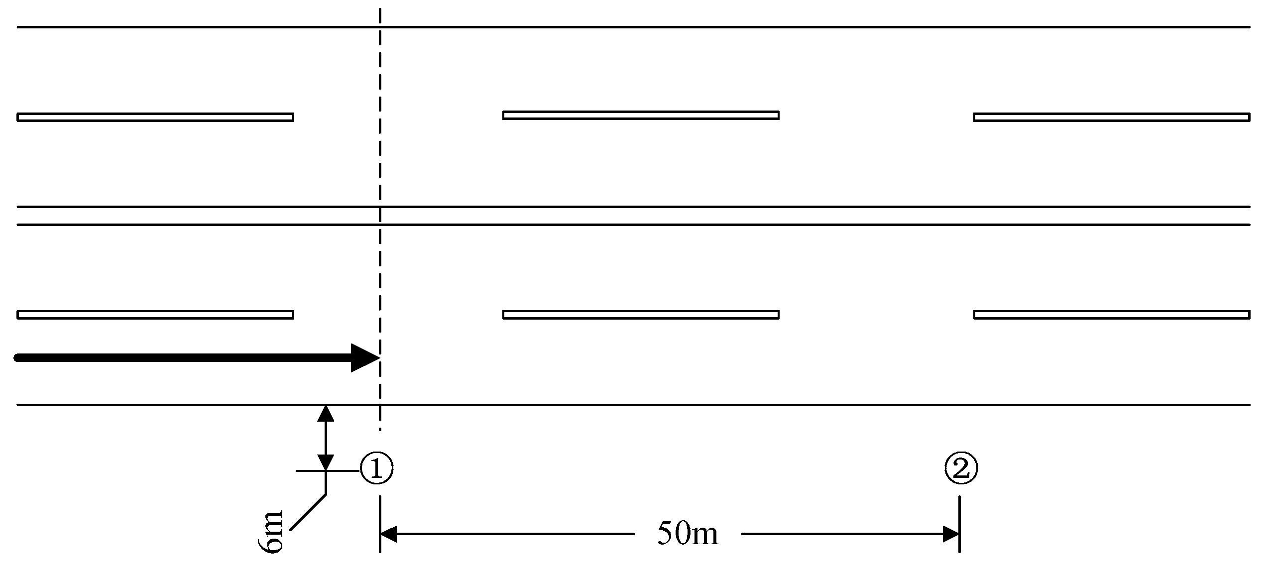
The measurements were conducted on the roadside of seven typical dry roads in Guangzhou, China, with a surface constructed of asphalt concrete. The parameters of surface could refer to the Chinese standard JTG F40-2004 (Technical Specification for Construction of Asphalt Pavements) [33]. To avoid possible disturbances, the samples were collected in places far away from intersections, rivers, and populated areas. The chosen urban roads have the following speed limits: 2 roads with 70 km/h, 3 roads with 60 km/h, 1 road with 50 km/h, and 1 road with 40 km/h. The spectrum was captured when the A-weighted sound pressure level during a vehicle pass-by was at its maximum, and the sampling frequency of sound level meter was 23 Hz, i.e., 23 spectra per second. Only one vehicle was measured at a time. In Figure 1, the locations of the measurement sites are shown. Both sites were 1.2 m high and 6 m to the roadside with a distance of 50 m to each other. In the experiment, the subject vehicles only moved from left to right alone. As the single vehicle passed by measurement site 1, the noise spectrum data were recorded by a digital noise recorder. The vehicle speed had little variation between points 1 and 2 while traveling on a long-straight road with a very sparse traffic flow. The vehicle speed was detected by a laser speedometer at measurement site 2.
In this paper, the vehicles are classified into three categories: heavy cars, middle cars, and light cars. The 1/3rd-octave-band sound pressure level (SPL) and the total SPL are included in the noise spectral data. All the noise data are A-weighted.
In this paper, 1351 sets of valid data were collected, among which 973 sets were light car data, 166 sets were middle car data, and 212 sets were heavy car data. The distribution of the samples is shown in Table 1.
2.2. Noise Spectra of Different Vehicle Types and Speeds
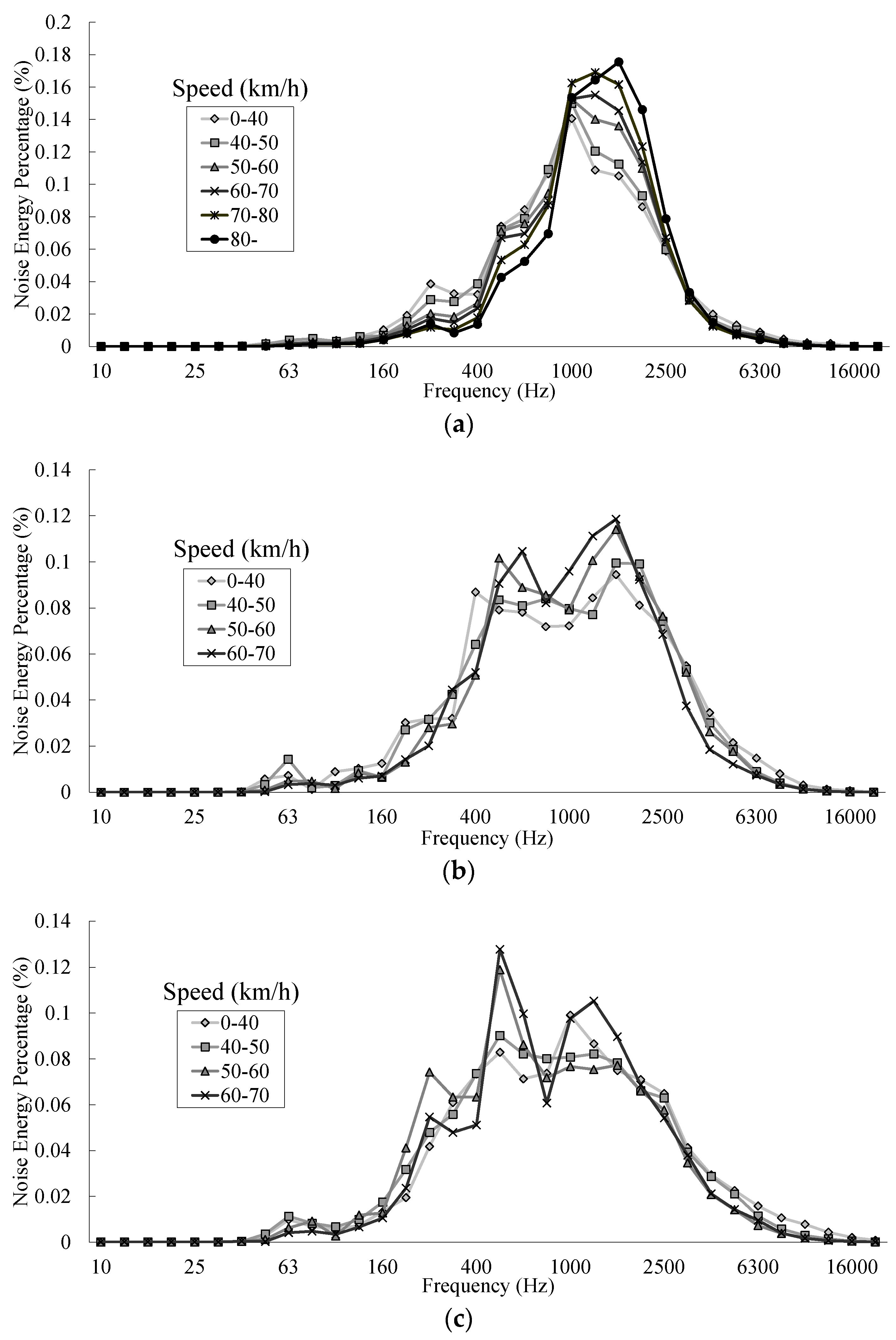
To analyze the frequency characteristics of traffic noise of different types of vehicle with various speed, the 1/3rd octave band spectrum data of vehicles were recorded, including 34 frequencies from 10 Hz to 20,000 Hz. To facilitate the analysis of the frequency characteristics, the following ranges are defined: frequencies from 10 Hz to 315 Hz are low frequency; 400 Hz to 800 Hz are medium-low frequency; 1000 Hz to 2500 Hz are medium-high frequency; 3150 Hz to 20,000 Hz are high frequency. To analyses the frequency characteristics of traffic noise and exclude the effect of SPL, the noise energy percentage of the 1/3rd octave band spectrum was calculated [34], as given by the following formulas (Equations (1)–(3)):
where is the number of vehicles, is the number of frequencies; is the SPL (dB), is the relative value of noise energy (dimensionless quantities), is the noise energy percentage (%), and is the mean percentage of noise energy (%).
From the equations, the SPL of each frequency of each vehicle is transformed to the noise energy percentage of each frequency. Figure 2 depicts the average noise energy percentage versus frequency for each type of vehicle with different speeds.
As shown in Figure 2, the noise energy percentage of the different speeds of three types of vehicles were performed with the 1/3rd octave band spectrum frequencies in the range of 10–20,000 Hz. The following points can be made:
- For a light vehicle, the noise energy is concentrated in the range of 500–2500 Hz, with peak frequency at approximately 1250 Hz. For a middle vehicle, the noise energy is concentrated in the range of 315–2500 Hz, with peak frequency at approximately 1600 Hz. For a heavy vehicle, the noise energy is concentrated in the range of 315–2500 Hz, with peak frequency at approximately 500 Hz.
- Speed will affect the SPL of a vehicle and the frequency characteristics of a vehicle. Noise spectra exhibit a trend of concentrating as the speed increase. Take the light vehicle case as an example, the noise energy percentage at the primary frequency range of 1000 Hz to 2500 Hz increases with speed, whereas the percentage of insignificant frequencies, such as low and medium-low frequencies, decrease with speeds. In addition, the main frequencies increase as the speed grows, especially for a light vehicle.
- The noise frequencies of the heavy vehicles are mainly medium-low frequency and medium-high frequency, which is quite different from the noise frequencies of light and middle vehicles, as their frequencies are mainly medium-high frequency.
- The emission noise of a vehicle can be divided into engine noise and tire/asphalt noise. Most of the light vehicles have gasoline engines. The contribution of engine noise is far less than the tire/asphalt noise. The proportion of diesel engines is high when for middle vehicles and heavy vehicles. The noise caused by diesel engine represents a large proportion, leading to a bi-modal trend in the noise spectra, which is in agreement with the rules presented by previous studies [34,35].
2.3. The Calculation Method of Insertion Loss
The center frequency with the minimum mean deviation between the 1/3rd-octave-band diffraction and the total diffraction is the equivalent frequency [36]. The equivalent frequency could be used in the approximate calculation of barrier attenuation. The results of the approximate calculation are close to the direct calculation using the whole spectrum as parameters, and the total error is always less than 1 dB. The procedures for calculating the insertion loss in this paper are presented below. Generally, several path length differences were preset first to calculate the 1/3rd-octave-band diffraction and the total diffraction. The detailed calculations are shown as follows:
- (1)
- Seven path length differences from 0.01 m to 10 m were preset first: 0.01 m, 0.1 m, 0.5 m, 1 m, 2.5 m, 5 m, 10 m;
- (2)
- The data were collected at the noise measurement site without the noise reduction effect of the barrier, and contained the 1/3rd-octave-band SPL and the total SPL L, where i is the sequence number of the 1/3rd-octave-band center frequency;
- (3)
- Through the diffraction formula, the diffraction of every 1/3rd-octave-band center frequency could be calculated as follows (Equation (4)):where is the path length difference and f is the 1/3rd-octave-band center frequency;
- (4)
- For a certain path length difference, the total SPL with the reduction effect of noise barrier can be calculated as (Equations (5) and (6))where is the 1/3rd-octave-band SPL with the reduction effect of barrier;
- (5)
- The following equation is used to yield the total diffraction (Equation (7)):
- (6)
- After calculating the total diffraction and the 1/3rd-octave-band diffraction with seven preset path length differences, the mean deviation between and can be obtained (Equation (8)).
3. Experimental Verification
Two verifying experiments were conducted: an insertion loss experiment and a distance attenuation experiment. In the experiments, vehicle noise was recorded next to the roads and subsequently played in the audio amplifier to emulate a point sound source that was used to measure actual insertion loss of noise barrier. For every type of car at different speed range, the synthesized point source consisted of five recorded audio samples. The length of each audio sample is 8 s.
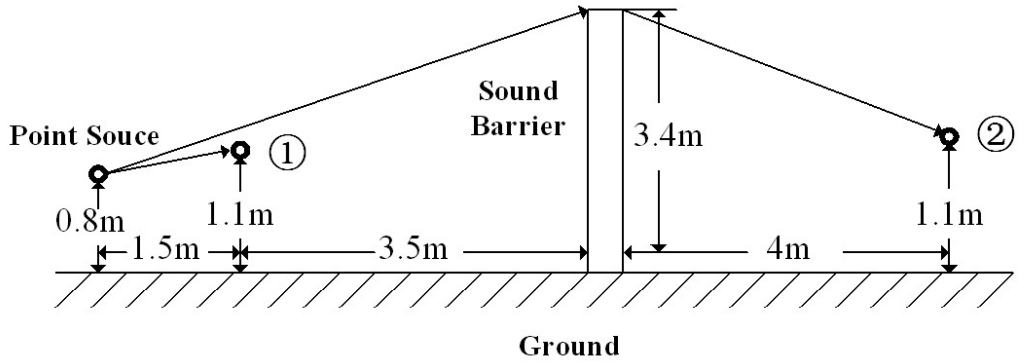
The insertion loss experiment was conducted to collect sound level pressure data in front of and behind the noise barrier. A schematic of the experiment is shown in Figure 3.
Two noise recorders were installed, one at measurement site 1 and the other at measurement site 2, to collect noise data and compute the noise levels and , respectively. The insertion loss of barrier is the difference between and . The computed equivalent noise levels are shown in Table 2.
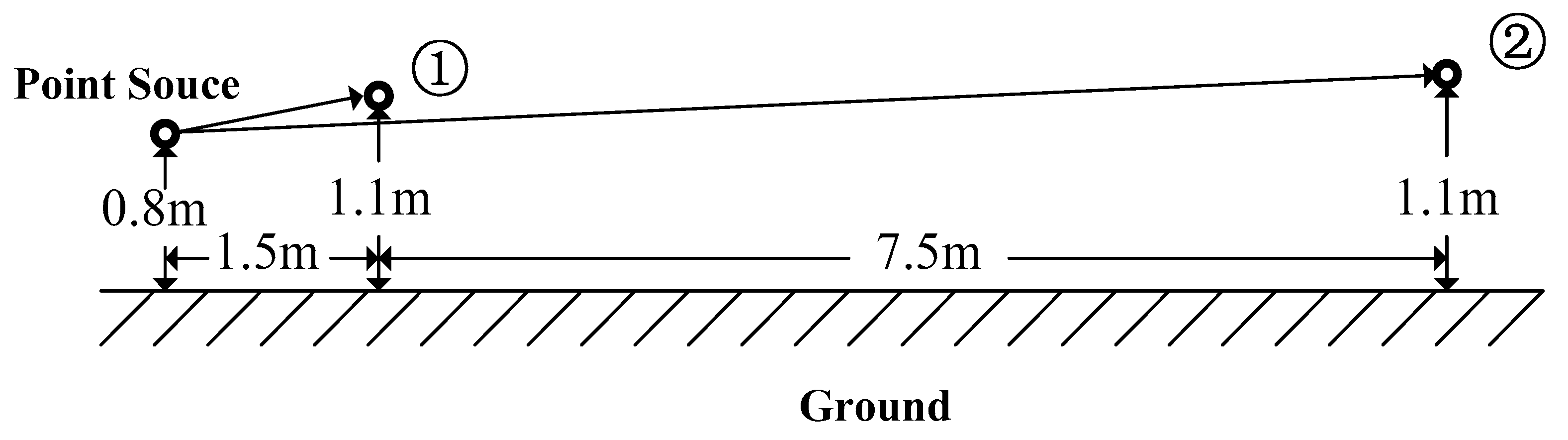
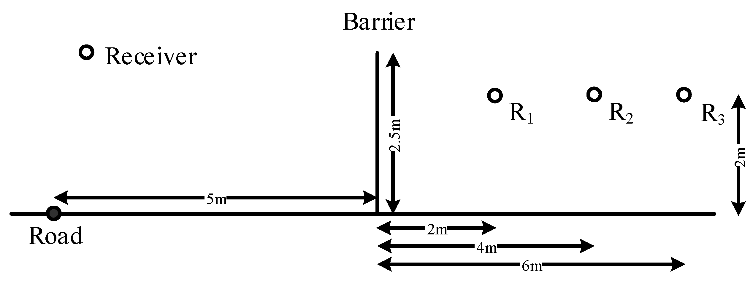
To obtain the actual value of diffraction, noise attenuation as a function of distance between the two measurement sites should be considered. The noise data were measured in an open space near the sound barrier to avoid possible errors introduced by the change of the experimental locations. Because noise attenuation with distance is independent of the frequency of the sound source [20], the sound source audios were merged into three categories in the experiment: heavy car, middle car, and light car. The geometric configuration of measurement is shown in Figure 4.
Noise recorders were installed in measurement site 1 and measurement site 2. The data are summarized in Table 3. Noise attenuation with distance for heavy, middle, and light vehicles are 11.16 dB, 11.03 dB, and 11.13 dB, respectively. The average of the three is defined as . In this instance, = 11.11 dB.
From the experimental verification, the actual value of diffraction by barrier was determined as follows (Equation (9)):
The theoretical value of diffraction is defined as (Equation (10))
where is the Fresnel number, .
Equations (9) and (10) are mainly applied to near-field conditions. According to reference [20], Equation (11) should be satisfied (Equation (11)).
where D is the distance from the sound source to the receivers’ center, d is the step of the receivers, and is the wave length. The speed of sound is 340 m/s.
In the experiment, D is calculated as approximately 5.26 m, d is set as 0.5 m in environmental acoustics calculation, and the wave length is in a range of [2.125, 0.054] with a primary frequency range of 160 Hz to 6300 Hz. Thus, Equation (11) is satisfied. The experimental setup can be considered with the theoretical formulation of the Fresnel number N.
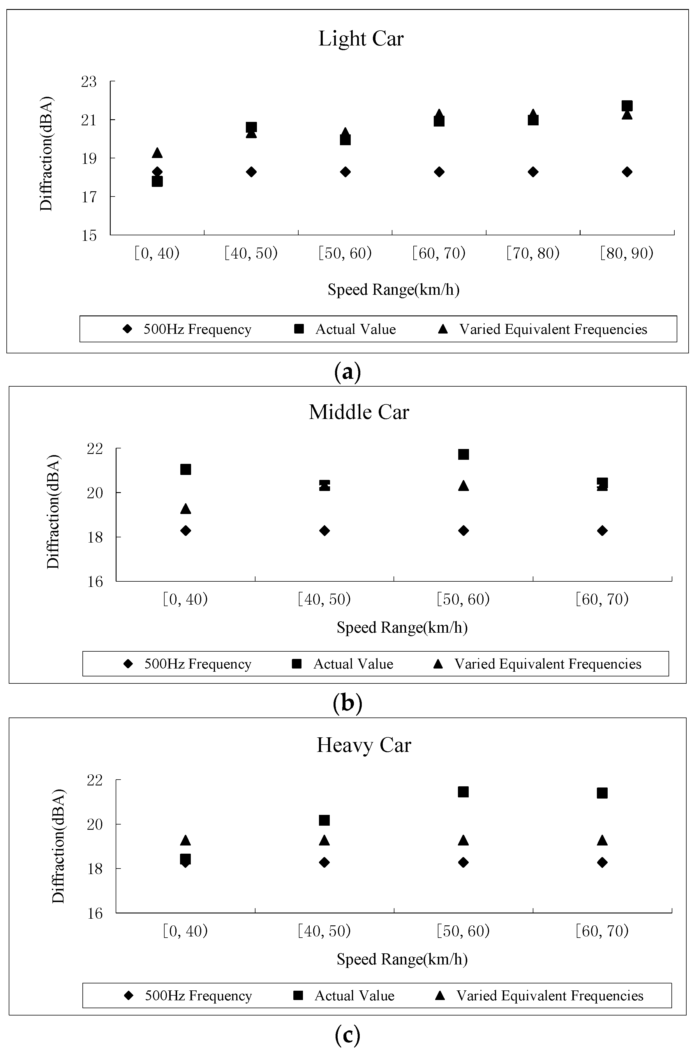
Two types of equivalent frequencies were used to yield the theoretical value of diffraction: one was the 500 Hz frequency, and the other was the varied equivalent frequencies computed in this paper. The actual value and the theoretical values are shown in Figure 5. The figure reveals that the error of diffraction calculated with the variety of noise equivalent frequencies is less than that calculated with 500 Hz frequency alone. Under the same experimental conditions, the average error using the 500 Hz frequency is approximately 2.3 dB, whereas the average error with the variety of noise equivalent frequencies is approximately 0.9 dB. With a difference of approximately 1.4 dB, the accuracy of the proposed method in calculating the noise barrier diffraction is undoubtedly more justified.
4. Effects of a Road Noise Barrier with Different Flow States
As shown in Figure 6, there is a two-dimensional sound field involving a sufficiently long enough sound barrier and a line road traffic noise source that is parallel to both the sound barrier and the ground. Three receivers (R1, R2, and R3) are chosen to analyze the effect of a road noise barrier with different type constituents and flow speed; all the receivers are sheltered by the barrier. The insertion losses of all receivers are calculated with different flow speed and the proportion of heavy vehicles. For each point, the SPL is calculated. The insertion loss of barrier can be defined as (Equation (12))
where SPL0 is the SPL at the receiver when the barrier is absent and SPLb is the SPL at the same receiver when the barrier is present.
LD = SPL0−SPLb
4.1. Effect of Vehicle Type
Traffic noise caused by heavy vehicles is quite different in frequencies compared to other vehicles based on the results of Section 2.2. Hence, the effects of the proportion of heavy vehicles on insertion loss of barrier were analyzed. The speed of the vehicles in this part is set as 50 km/h, and the flow of 1000 vehicles per hour consists of light and heavy vehicles with 11 different proportions. To ensure that the results are not affected by the different vehicles’ sound source strong, the emission intensity of each vehicle source is set as 85 dB. Traffic noise for different heavy vehicle proportions (0, 10%, 20%, 30%, 40%, 50%, 60%, 70%, 80%, 90%, and 100%) on each point was calculated.
With different proportions of heavy vehicles, the insertion losses at three points are shown in Figure 7. LD presents a distinct pattern regarding points R1, R2, and R3, and the insertion loss at all of the receivers have relationships with the proportion of heavy vehicles. For point 1, LD and heavy vehicles a (%) follow the linear relationship of LD = −0.0293a + 24.661, i.e., 10 percent of heavy vehicles can cause a 0.29 dB decline on insertion loss in this scene. The results show that the SPL behind a barrier of a heavy vehicle flow is approximately 2.3 dB higher than that a light vehicle flow with the same source emission intensity. The same rule is also applicable to the overall shadow area. The heavy vehicles have more acoustical constituents at low frequencies compared to light vehicles, which are more significantly shaded by barriers. The insertion loss of heavy vehicle flow is the highest, followed by the insertion loss of mixed traffic flow, and the insertion loss of light vehicle flow is the lowest; this result indicates that the lower-frequency sound can bypass the barrier more easily. Thus, flow control of heavy vehicles whose sound is concentrated in low frequencies is an effective measure to improve the acoustic environment near roadways.
4.2. Effect of Flow Speed
Vehicle noise characteristics of various speeds are different in frequencies according to the results of Section 2.2. Hence, the effects of different traffic flow speeds on the insertion loss of a noise barrier were analyzed. The flow of 1000 vehicles per hour consists of light and heavy vehicles with seven different flow speeds. The emission intensity of each vehicle source is set as 85 dB. Traffic noise with different traffic flow speeds (30 km/h, 40 km/h, 50 km/h, 60 km/h, 70 km/h, 80 km/h, and 90 km/h) on each point was calculated. Light vehicle flow, middle traffic flow, heavy vehicle flow, and mixed traffic flow (with 30% heavy vehicles) were considered in this section.
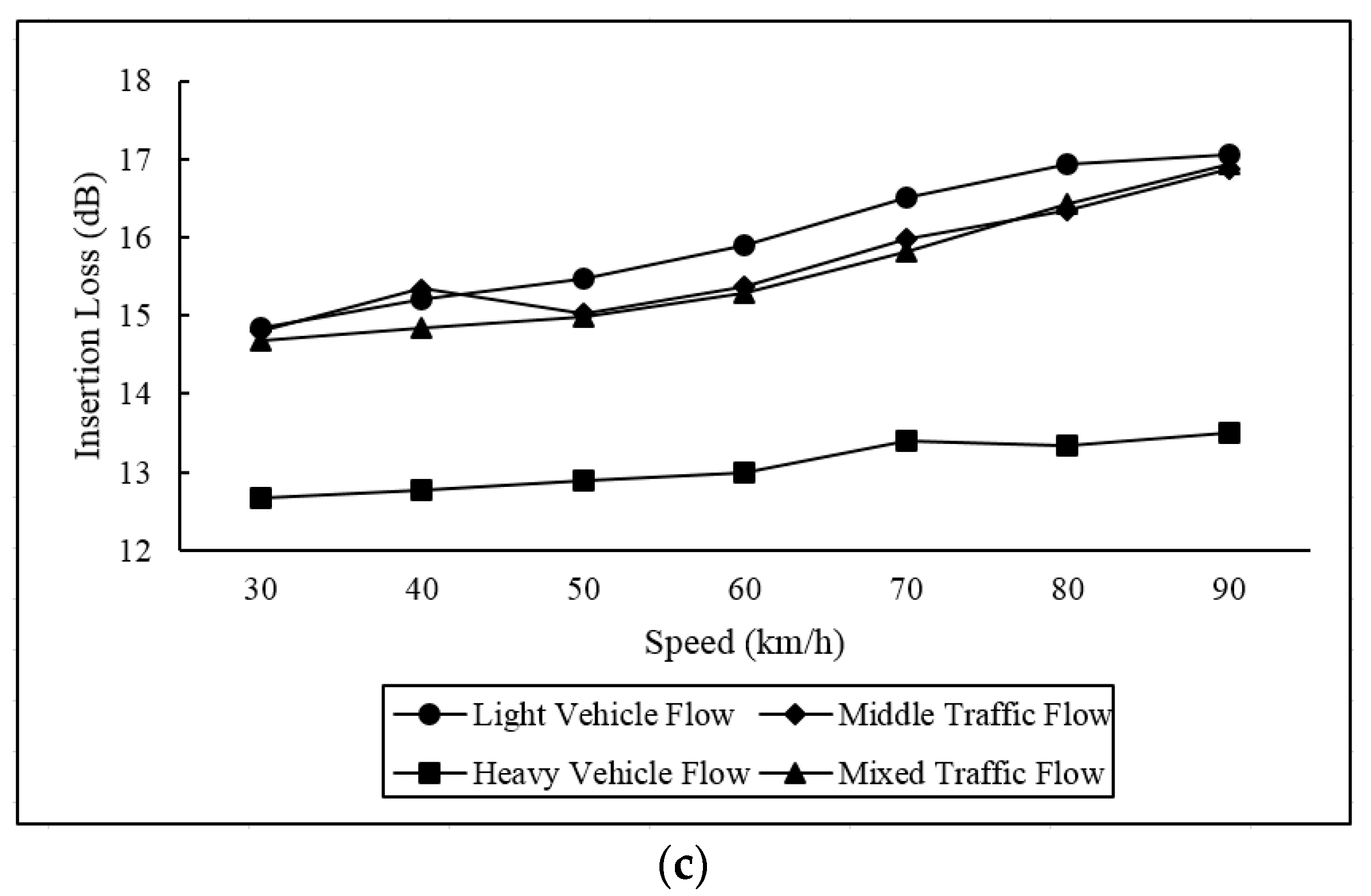
With different type constituents and speeds of traffic flow, the insertion losses at three points are shown in Figure 8. From the results of the calculated LD values, the analysis is as follows:
- The insertion losses of barrier increase with the flow speeds grow at all chosen points, regardless of the composition of vehicle types. For example, when the speed is below 40 km/h, the insertion loss of light vehicle flow at R1 is approximately 23.7 dB, and the insertion loss increases non-linearly as the speed increases. At the speed of 90 km/h, the LD value reached approximately 26.3 dB.
- Figure 8 clearly shows that the noise barrier has sound-shading effects in all situations. The trend of increase of insertion loss with speed is observed, and the trend is considerably more obvious for light vehicle flow, middle traffic flow, and mixed traffic flow compared to heavy vehicle flow. The added LD value at R1 of a 30–90 km/h speed range of light vehicle flow, middle traffic flow, and mixed traffic flow is 2.65 dB, 1.73 dB, and 2.33 dB, respectively. However, the added insertion loss value of the same speed range of heavy vehicle flow is only 0.36 dB, which is considerably smaller. The data at R2 and R3 present the same rule because the main acoustics of light vehicle and middle vehicle are shifted to higher frequencies, whereas the main acoustics of heavy vehicle are slightly changed in frequency.
- From the values, the SPL behind a barrier of a common mixed traffic flow with high speed is approximately 2 dB lower than the level with a low speed with the same source emission intensity. For a heavy vehicle flow, the sound pressure levels behind a barrier are little different with high or low flow speed.
5. Conclusions
A method for insertion loss calculation of a road noise barrier based on frequencies was presented in this paper. The proposed method realizes a more accurate calculation compared to the commonly used method based on a single 500-Hz sound. Several path length differences were preset to calculate the 1/3rd-octave-band diffraction and the total diffraction. Using different weights of spectrum according to the experimental noise data and traffic flow state, the insertion loss can be accurately calculated.
The method was verified by experiments with approximately 1.4 dB improvement in accuracy. The varied equivalent frequencies can be applied in the microscopic simulation of traffic noise, in which all different types of cars are considered to be the point source in the road network.
The noise protection of a road noise barrier with different flow states was analyzed based on a case study. The sound pressure level behind a barrier of a heavy vehicle flow is approximately 2.3 dB higher than that of a light vehicle flow with the same source emission intensity. The sound pressure level behind a barrier of a common mixed traffic flow with high speed is approximately 2 dB lower than the level with a low speed with the same source emission intensity. A road with high speed and high light vehicle proportion flow is recommended to establish a noise barrier.
Acknowledgments
This work was supported by the National Natural Science Foundation of China (No. 11574407) and the Fundamental Research Funds for the Central Universities (No. 17lgpy55).
Author Contributions
This paper is a result of the full collaboration of all the authors. Ming Cai and Haibo Wang conceived and designed the experiments; Peng Luo performed the experiments; Haibo Wang and Peng Luo analyzed the data; Haibo Wang wrote the paper.
Conflicts of Interest
The authors declare no conflict of interest.
References
- Dehrashid, S.S.A.; Nassiri, P. Traffic noise assessment in the main roads of Sanandaj, Iran. J. Low Freq. Noise Vib. Act. Control 2015, 34, 39–48. [Google Scholar] [CrossRef]
- Garacia, J.S.; Solano, J.J.P.; Serrano, M.C.; Camba, E.A.N.; Castel, S.F.; Asensi, A.S.; Suay, F.M. Spatial statistical analysis of urban noise data from a WASN gathered by an IoT system: Application to a small city. Appl. Sci. Basel 2016, 6, 380. [Google Scholar] [CrossRef]
- Morel, J.; Marquisfavre, C.; Dubois, D.; Pierrette, M. Road traffic in urban areas: A perceptual and cognitive typology of pass-by noises. Acta Acust. United Acust. 2012, 98, 166–178. [Google Scholar] [CrossRef]
- Di, G.Q.; Liu, X.Y.; Lin, Q.L.; Zheng, Y.; He, L.J. The relationship between urban combined traffic noise and annoyance: An investigation in Dalian, north of China. Sci. Total Environ. 2012, 432, 189–194. [Google Scholar] [CrossRef] [PubMed]
- Roswall, N.; Raaschou-Nielsen, O.; Ketzel, M.; Overvad, K.; Halkjær, J.; Sørensen, M. Modeled traffic noise at the residence and colorectal cancer incidence: A cohort study. Cancer Cause Control 2017, 28, 745–753. [Google Scholar] [CrossRef] [PubMed]
- Oiamo, T.H.; Luginaah, I.N.; Baxter, J. Cumulative effects of noise and odour annoyances on environmental and health related quality of life. Soc. Sci. Med. 2015, 146, 191–203. [Google Scholar] [CrossRef] [PubMed]
- Monazzam, M.R.; Fard, S.M.B. Performance of passive and reactive profiled median barriers in traffic noise reduction. Appl. Phys. Eng. 2011, 12, 78–86. [Google Scholar] [CrossRef]
- Reiter, P.; Wehr, R.; Ziegelwanger, H. Simulation and measurement of noise barrier sound-reflection properties. Appl. Acoust. 2017, 123, 133–142. [Google Scholar] [CrossRef]
- Monazzam, M.R.; Lam, Y.W. Performance of profiled single noise barriers covered with quadratic residue diffusers. Appl. Acoust. 2005, 66, 709–730. [Google Scholar] [CrossRef]
- Voropayev, S.I.; Ovenden, N.C.; Fernando, H.J.S.; Donovan, P.R. Finding optimal geometries for noise barrier tops using scaled experiments. J. Acoust. Soc. Am. 2017, 141, 722–736. [Google Scholar] [CrossRef] [PubMed]
- Ishizuka, T.; Fujiwara, K. Performance of noise barriers with various edge shapes and acoustical conditions. Appl. Acoust. 2004, 65, 125–141. [Google Scholar] [CrossRef]
- Arenas, J.P. Potential problems with environmental sound barriers when used in mitigating surface transportation noise. Sci. Total Environ. 2008, 405, 173–179. [Google Scholar] [CrossRef] [PubMed]
- Zhao, W.C.; Chen, L.L.; Zheng, C.J.; Liu, C.; Chen, H.B. Design of absorbing material distribution for sound barrier using topology optimization. Struct. Multidiscip. Optim. 2017, 56, 315–329. [Google Scholar] [CrossRef]
- Joynt, J. A Sustainable Approach to Environmental Noise Barrier Design. Ph.D. Thesis, University of Sheffield, Sheffield, UK, 2006. [Google Scholar]
- Kotzen, B.; English, C. Environmental Noise Barriers: A Guide to Their Acoustic and Visual Design; E & FN Spon-Routledge: London, UK, 1999. [Google Scholar]
- Sommerfeld, A. Mathematische theorie der diffraktion. Math. Ann. 1896, 47, 317–374. [Google Scholar] [CrossRef]
- Wang, H.B.; Cai, M.; Zhong, S.Q.; Li, F. Sound field study of a building near a roadway via the boundary element method. J. Low Freq. Noise Vib. Act. Control 2017, in press. [Google Scholar] [CrossRef]
- He, Z.C.; Li, G.Y.; Liu, G.R.; Cheng, A.G.; Li, E. Numerical investigation of ES-FEM with various mass redistribution for acoustic problems. Appl. Acoust. 2015, 89, 222–233. [Google Scholar] [CrossRef]
- Hiraishi, M.; Tsutahara, M.; Leung, R.C.K. Numerical simulation of sound generation in a mixing layer by the finite difference lattice Boltzmann method. Comput. Math. Appl. 2010, 59, 2403–2410. [Google Scholar] [CrossRef]
- Ma, D.Y.; Shen, H. Hankbook of Acoustics; SciPress: Beijing, China, 2004. [Google Scholar]
- Maekawa, Z. Noise reduction by screens. Appl. Acoust. 1968, 1, 157–173. [Google Scholar] [CrossRef]
- Yamamoto, K.; Takagi, K. Expressions of Maekawa’s chart for computation. Appl. Acoust. 1992, 37, 75–82. [Google Scholar] [CrossRef]
- Menounou, P. A correction to Maekawa’s curve for the insertion loss behind barriers. J. Acoust. Soc. Am. 2001, 110, 1828–1838. [Google Scholar] [CrossRef] [PubMed]
- Kurze, U.J.; Anderson, G.S. Sound attenuation by barriers. Appl. Acoust. 1971, 4, 35–53. [Google Scholar] [CrossRef]
- Cianfrini, C.; Corcione, M.; Fontana, L. Experimental verification of the acoustic performance of diffusive roadside noise barriers. Appl. Acoust. 2007, 68, 1357–1372. [Google Scholar] [CrossRef]
- Li, K.M.; Wong, H.Y. A review of commonly used analytical and empirical formulae for predicting sound diffracted by a thin screen. Appl. Acoust. 2005, 66, 45–75. [Google Scholar] [CrossRef]
- Anderson, G.S.; Menge, C.W.; Rossano, C.F.; Armstrong, R.E.; Ronning, S.A.; Fleming, G.G.; Lee, C.S.Y. FHWA traffic noise model, version 1.0: Introduction to its capacities and screen components. Wall J. 1996, 22, 14–17. [Google Scholar]
- Shu, N.; Cohn, L.F.; Kim, T.K. Improving traffic-noise model insertion loss accuracy based on diffraction and reflection theories. J. Transp. Eng. 2007, 133, 281–287. [Google Scholar] [CrossRef]
- Monazzam, M.R.; Nassiri, P. Contribution of quadratic residue diffusers to efficiency of tilted profile parallel highway noise barriers. Iran. J. Environ. Health Sci. Eng. 2009, 6, 271–284. [Google Scholar]
- Grubeša, S.; Domitrović, H.; Jambrošić, K. Performance of traffic noise barriers with varying cross-section. PROMET-Traffic Transp. 2011, 23, 161–168. [Google Scholar] [CrossRef]
- Huang, X.; Zou, H.; Qiu, X. A preliminary study on the performance of indoor active noise barriers based on 2D simulations. Build. Environ. 2015, 94, 891–899. [Google Scholar] [CrossRef]
- Chen, S.M.; Wang, D.F.; Liang, J. Sound quality analysis and prediction of vehicle interior noise based on grey system theory. Fluct. Noise Lett. 2012, 11, 1250016. [Google Scholar] [CrossRef]
- Ministry of Communications of the People’s Republic of China. Technical Specification for Construction of Asphalt Pavements; JTG F40-2004; Ministry of Communications of the People’s Republic of China: Beijing, China, 2005.
- Cai, M.; Zhong, S.Q.; Wang, H.B.; Chen, Y.X.; Zeng, W.X. Study of the traffic noise source intensity emission model and the frequency characteristics for a wet asphalt road. Appl. Acoust. 2017, 123, 55–63. [Google Scholar] [CrossRef]
- Zhang, Y.F. Road Traffic Environmental Engineering; China Communications Press: Beijing, China, 2001. [Google Scholar]
- Ministry of Environmental Protection of the People’s Republic of China. Norm on Acoustical Design and Measurement of Noise Barriers; HJ/T 90-2004; Ministry of Environmental Protection of the People’s Republic of China: Beijing, China, 2004.
Figure 1.
Locations of the Measurement Spots.

Figure 2.
Noise energy percentage with the 1/3rd octave band spectrum frequencies at different speeds of three types of vehicles. (a) light vehicles; (b) middle vehicles; (c) heavy vehicles.
Figure 2.
Noise energy percentage with the 1/3rd octave band spectrum frequencies at different speeds of three types of vehicles. (a) light vehicles; (b) middle vehicles; (c) heavy vehicles.

Figure 3.
Insertion loss experiment.

Figure 4.
Noise attenuation experiment with distance.

Figure 5.
Comparisons between 500 Hz frequency and the variety of equivalent frequencies for diffraction by barrier. (a) light vehicle; (b) middle vehicle; (c) heavy vehicle.
Figure 5.
Comparisons between 500 Hz frequency and the variety of equivalent frequencies for diffraction by barrier. (a) light vehicle; (b) middle vehicle; (c) heavy vehicle.

Figure 6.
A case of noise calculation behind a road sound barrier.

Figure 7.
Insertion loss of the road barrier with different proportions of heavy vehicles.

Figure 8.
Insertion loss of barrier with different flow speeds. (a) Point R1; (b) Point R2; (c) Point R3.
Figure 8.
Insertion loss of barrier with different flow speeds. (a) Point R1; (b) Point R2; (c) Point R3.


Table 1.
Distribution of the samples of vehicle noise spectra.
| Speed | Light Car | Middle Car | Heavy Car |
|---|---|---|---|
| [0, 40) km/h | 39 | 23 | 41 |
| [40, 50) km/h | 186 | 48 | 80 |
| [50, 60) km/h | 317 | 57 | 55 |
| [60, 70) km/h | 222 | 38 | 36 |
| [70, 80) km/h | 134 | ||
| ≥80 km/h | 75 |
Table 2.
Noise levels computed in the insertion loss experiment (dB).
| Speed (km/h) | Light Car | Middle Car | Heavy Car | |||
|---|---|---|---|---|---|---|
| [0, 40) | 75.21 | 46.31 | 84.26 | 52.11 | 83.91 | 54.38 |
| [40, 50) | 80.69 | 48.98 | 83.85 | 52.42 | 80.12 | 48.84 |
| [50, 60) | 80.09 | 49.03 | 86.59 | 53.76 | 85.95 | 53.39 |
| [60, 70) | 82.17 | 50.14 | 85.53 | 53.99 | 86.68 | 54.17 |
| [70, 80) | 82.74 | 50.65 | ||||
| ≥80 | 85.30 | 52.48 | ||||
Table 3.
Data collected in the noise attenuation experiment with distance (dB).
| Vehicle Type | |||
|---|---|---|---|
| Light Car | 82.02 | 70.86 | 11.16 |
| Middle Car | 84.13 | 73.10 | 11.03 |
| Heavy Car | 84.02 | 72.89 | 11.13 |
© 2018 by the authors. Licensee MDPI, Basel, Switzerland. This article is an open access article distributed under the terms and conditions of the Creative Commons Attribution (CC BY) license (http://creativecommons.org/licenses/by/4.0/).
Share and Cite
MDPI and ACS Style
Wang, H.; Luo, P.; Cai, M. Calculation of Noise Barrier Insertion Loss Based on Varied Vehicle Frequencies. Appl. Sci. 2018, 8, 100. https://doi.org/10.3390/app8010100
AMA Style
Wang H, Luo P, Cai M. Calculation of Noise Barrier Insertion Loss Based on Varied Vehicle Frequencies. Applied Sciences. 2018; 8(1):100. https://doi.org/10.3390/app8010100
Chicago/Turabian StyleWang, Haibo, Peng Luo, and Ming Cai. 2018. "Calculation of Noise Barrier Insertion Loss Based on Varied Vehicle Frequencies" Applied Sciences 8, no. 1: 100. https://doi.org/10.3390/app8010100
Note that from the first issue of 2016, this journal uses article numbers instead of page numbers. See further details here.