
Application of Machine Learning for the Spatial Analysis of Binaural Room Impulse Responses


Communication Technologies Research Group, Department of Electronic Engineering, University of York, York YO10 5DD, UK
*
Author to whom correspondence should be addressed.
†
Current address: Audio Lab, Department of Electronic Engineering, University of York, York YO10 5DD, UK.
‡
Binaural model code, neural network code, and direct sound and reflection dataset will be made available at: 10.5281/zenodo.1038021.
Appl. Sci. 2018, 8(1), 105; https://doi.org/10.3390/app8010105
Submission received: 30 October 2017
/
Revised: 12 December 2017
/
Accepted: 26 December 2017
/
Published: 12 January 2018
(This article belongs to the Special Issue Sound and Music Computing)
Abstract
:Spatial impulse response analysis techniques are commonly used in the field of acoustics, as they help to characterise the interaction of sound with an enclosed environment. This paper presents a novel approach for spatial analyses of binaural impulse responses, using a binaural model fronted neural network. The proposed method uses binaural cues utilised by the human auditory system, which are mapped by the neural network to the azimuth direction of arrival classes. A cascade-correlation neural network was trained using a multi-conditional training dataset of head-related impulse responses with added noise. The neural network is tested using a set of binaural impulse responses captured using two dummy head microphones in an anechoic chamber, with a reflective boundary positioned to produce a reflection with a known direction of arrival. Results showed that the neural network was generalisable for the direct sound of the binaural room impulse responses for both dummy head microphones. However, it was found to be less accurate at predicting the direction of arrival of the reflections. The work indicates the potential of using such an algorithm for the spatial analysis of binaural impulse responses, while indicating where the method applied needs to be made more robust for more general application.
1. Introduction
A Binaural room impulse response (BRIR) is a measurement of the response of a room to an excitation from an (ideally) impulsive sound. The BRIR is comprised of the superposition of the direct source-to-receiver sound component, discrete reflections produced from interactions with a limited number of boundary surfaces, together with the densely-distributed, exponentially-decaying reverberant tail that results from repeated surface interactions. In particular, a BRIR is characterised by the receiver having the properties of a typical human head, that is two independent channels of information separated appropriately, and subject to spatial variation imparted by the pinnae and head. Therefore, the BRIR is uniquely defined by the location, shape and acoustic properties of reflective surfaces, together with the source and receiver position and orientation.
The BRIR is therefore a representation of the reverberant characteristics of an environment and is commonly used throughout the fields of acoustics and signal processing. Through the use of convolution, the reverberant characteristics of the room, as captured within the BRIR, can be imparted onto other audio signals, giving the perception of listening to that audio signal as if it were recorded in the BRIR measurement position. This technique for producing artificial reverberation has numerous applications, including: music production, game sound design, alongside other audio-visual media. In acoustics, the spatiotemporal characteristics of reflections arising from sound propagation and interaction within a given bounded space can be captured through measuring the room impulse response for a given source/receiver pair. One problem associated with this form of analysis is obtaining a prediction for the direction of arrival (DoA) of these reflections. Understanding the DoA of reflections can allow for the formulation of reflection backpropagation and geometric inference algorithms, amongst other features, that reveal the properties of the given acoustic environment for which the impulse response was obtained. This has applications in robot audition, sound source localisation tasks, as well as room acoustic analysis, treatment and simulation. These algorithms can be used to develop an understanding of signal propagation in a room, allowing the point of origin for acoustic events arriving at the receiver to be found. This knowledge of the signal propagation in the environment can then be used to acoustically treat the environment, improving the perceptibility of signals produced within the environment. Conversely, the inferred geometry can be used to simulate the acoustic response of the room to a different source and receiver through the use of computational acoustic simulation techniques.
Existing methods [1,2,3] have approached reflection DoA estimation using four or more channels, while methods looking at localising the components in two-channel BRIRs have generally shown poor accuracy for predicting the DoA of the reflections in these BRIRs [4]. This paper investigates a novel approach to using neural networks for DoA estimation for the direct and reflected sound components in BRIRs. The reduction in the number of channels available for analyses significantly adds to the complexity of extracting highly accurate direction of arrival predictions.
The human auditory system is a complex, but robust system, capable of undertaking sound localisation tasks under varying conditions with relative ease [5]. The binaural nature of the auditory system leads to two main interaural localisation cues: interaural time difference (ITD), the time of arrival difference between the signals arriving at the two ears, and interaural level difference (ILD), the frequency-dependent difference in signal loudness at the two ears due to the difference in propagation path and acoustic shadowing produced by the head [5,6]. In addition to these interaural cues, it has been shown that the auditory system makes use of self-motion [7] and the spectral filtering produced by the pinnae to improve localisation accuracy, particularly with regards to elevation and front-back confusion [5,8].
Given the robustness of the auditory system at performing localisation tasks [5], it should be possible to produce a computational approach using the same auditory cues. Due to the nature of the human auditory system, machine-hearing approaches are often implemented in binaural localisation algorithms, typically using either Gaussian mixture models (GMMs) [9,10,11] or neural networks (NNs) [12,13,14,15]. In most cases, the data presented to the machine-hearing algorithm fit into one of two categories: binaural cues (ITD and ILD) or spectral cues. Previous machine-hearing approaches to binaural localisation have shown good results across the training data and, in some cases, good generalisability across unknown data from different datasets [9,10,11,12,13,14,15].
In [14], a cochlear model was used to pre-process head-related impulse responses (HRIRs), the output of which was then used to calculate the ITD and ILD. Two different cochlear models for ITD and ILD calculation were used, as well as feeding the cochlear model output to the NN. The results presented showed that the NN was able to build up a spatial map from raw output of the cochlear model, which performed better under test conditions than using the binaural cues calculated from the output of the cochlea model.
Backman et al. [13] used a feature vector comprised of the cross-correlation function and ILD to train their NNs, which were able to produce highly accurate results within the training data. However, upon presenting the NN with unknown data, it was found to have poor generalisation.
In [12], Palomäki et al. presented approaches using a self-organising map and a multi-layer perceptron trained using the ITD and ILD values calculated from a binaural model. They found that both were capable of producing accurate results within the training data, with the self-organising map requiring the addition of head rotation to help disambiguate cue similarity between the front and back hemispheres [12]. Their findings suggested that a much larger dataset is required to achieve generalisation with the multi-layer perceptron.
In [9,10,11], GMMs trained using the ITD and ILD were used to classify the DoA. In both cases, the GMMs were found to produce accurate azimuthal DoA estimates. Their findings showed that the GMM’s ability to accurately predict azimuth DoA was affected by the source and receiver distance and the reverberation time, with larger source-receiver distances and reverberation times generally reducing the accuracy of the model [9,10]. The results presented in [9] showed that a GMM trained with a multi-conditional training (MCT) dataset was able to localise a signal using two different binaural dummy heads with high accuracy.
Ding et al. [16] used the supervised binaural mapping technique, to map binaural features to 2D directions, which were then used to localise a sound source’s azimuth and elevation position. They presented results displaying the effect of reverberation on prediction accuracy, showing that prediction accuracy decreased as reverberation times increased. They additionally showed that the use of a binaural dereverberation technique improved prediction accuracy across all reverberation times [16].
Recent work by Ma et al. [15] compared the use of GMM and deep NNs (DNNs) for the azimuthal DoA estimation task. The DNN made use of head rotation produced by a KEMAR unit (KEMAR: Knowles Electronics Manikin for Acoustic Research) is a head and torso simulator designed specifically for, and commonly used in, binaural acoustic research) [17] fitted with a motorised head. It was found that the addition of head rotation reduced the ambiguity between front and back and that DNNs outperformed GMMs, with DNNs proving better at discerning between the front and back hemispheres.
Work presented by Vesa et al. [4] investigated the problem of DoA analysis of the component parts of a BRIR. They used the continuous-wavelet transform to create a frequency domain representation of the signal, which is used to compute the ILD and ITD across frequency bands. The DoA is then computed by iterating over a database of reference HRIRs and finding the reference HRIR with the closest matching ILD and ITD values to the component of the BRIR being analysed; the DoA is then assumed to be the same as the reference HRIR. They reported mean angular errors between 28.7° and 54.4° for the component parts of the measured BRIRs.
This paper presents a novel approach for the spatial analysis of two-channel BRIRs, using a binaural model fronted NN to estimate the azimuthal direction of arrival for the direct sound and reflected components (direct sound is used to refer to the signal emitted by a loudspeaker arriving at the receiver, and the reflected component refers to a reflected copy of the emitted signal arriving at the receiver after incidence with a reflective surface) of the BRIRs. It develops and extends the approach adopted in [15] in terms of the processing used by the binaural model to extract the interaural cues, the use of a cascade-correlation neural network as opposed to the multi-layer perceptron to map the binaural cues to the direction of arrival classes, the nature of the sound components being analysed—short pulses relating to the direct sound and reflected components of a BRIR as opposed to continuous speech signals—and the method by which measurement orientations are implemented and analysed by the NN. In this paper, multiple measurement orientations are presented simultaneously to the NN, whereas in [15], multiple orientations are presented as rotations produced by a motorised head with the signals being analysed separately by the NN, which allowed for active sound source localisation in an environment.
The following sections are organised as follows; in Section 2, the implementation of the binaural model and NN, the data model used and the methodology used to generate a test dataset are discussed; Section 3 presents the test results; Section 4 discusses the findings; and Section 5 concludes the paper.
2. Materials and Methods
The proposed method uses a binaural model to produce representations of the time of arrival and frequency-dependent level differences between the signals arriving at the left and right ear of a dummy head microphone. This binaural model is used to produce a set of interaural cues for the direct sound and each detectable reflection within a BRIR. These cues alone are not sufficient to provide accurate localisation of sound sources, due to interaural cue similarities observed at mirrored source positions in the front/rear hemispheres. To distinguish between sounds arriving from either the front or rear of the head, an additional set of binaural cues is generated for the corresponding direct sound and reflected component of a BRIR captured with the dummy head having been rotated by °. Presenting the NN with both the original measurement and one captured after rotating the receiver helps reduce front-back confusions, arising due to similarities in binaural cues for positions mirrored in the front and back hemispheres. The use of a rotation of ° was used in this study based on tests run with different rotation angles, which are presented in Section 2.2. These sets of interaural cues are then interpreted by a cascade-correlation NN, producing a prediction of the DoA for the direct sound and each detected reflection in the BRIR. The NN is trained with an MCT dataset of interaural cues extracted from HRIRs measured with a KEMAR 45BC binaural dummy head microphone, with added simulated spatially white noise at different signal-to-noise ratios. The NN is trained using mini-batches of the training dataset, and optimised using the adaptive moment (ADAM) optimiser; with the order of the training data randomised at the end of the training iteration.
2.1. Binaural Model
A binaural model inspired by the work presented in [18,19] is used to compute the temporal and frequency-dependent level differences between the signals arriving at the left and right ears of a listener. Both the temporal and spectral feature spaces provide directionally-dependent cues, produced by path differences between ears and acoustic shadowing produced by the presence of the head, which allow the human auditory system to localise a sound source in an environment [6,20]. These directionally-dependent feature spaces are used in this study to produce a feature vector that can be analysed by an NN to estimate the direction of arrival.
Prior to running the analysis of the binaural signals, the signal vectors being analysed are zero-padded by 2000 samples accounting for signal delay introduced by the application of a gammatone filter bank. This ensures that no part of the signal is lost when dealing with small windows of sound, where the filter delay would push the signal outside of the represented sample range. The zero-padded signals are then passed through a bank of 64 gammatone filters spaced equally from 80 Hz to 22 kHz using the equivalent rectangular bandwidth scale. The gammatone filter implementation in Malcolm Slaney’s ‘Auditory Toolbox’ [21] was used in this study. The output of the cochlea is then approximated using the cochleagram function in [22] with a window size of six samples and an overlap of one sample; this produces an map of auditory nerve firing rates across time-frequency units, where N is the number of time samples and F is the number of gammatone filters. The cochleagram is calculated as:
where is the cochleagram output for the left channel for gammatone filter f at frame number n, is the filtered left channel of audio at gammatone filter f and time frame , which is six samples in length and signifies vector transposition [22]. The cochleagram was used to extract the features as opposed to extracting directly from the gammatone filters, as it was found to produce more accurate results when passed to the NN.
The interaural cues are then computed across the whole cochleagram producing a single set of interaural cues for each binaural signal being analysed. The first of these interaural cues is the interaural cross-correlation (IACC) function, which is computed for each frequency band as the cross-correlation between the whole approximated cochlea output and for the left and right channel, respectively, with a maximum lag of ms. The maximum lag of ms was chosen based on the maximum time delays suggested by Pulkki et al. for their binaural model proposed in [18]. The cross-correlation function is then normalised by,
where is the cross-correlation between the left and right approximated cochlea outputs for gammatone filter f. The IACC is then averaged across the 64 gammatone filters, producing the temporal feature space for the analysed signal. The maximum peak in the IACC function represents the signal delay between the left and right ear. The decision to use the entire IACC function as opposed to the ITD was based on the findings presented in [15], which suggested that features within the IACC function, such as the relationship between the main peak and any side bands, varied with azimuthal direction of arrival.
The ILD is then calculated from the cochleagram output in decibels as the loudness ratio between the two ears for each gammatone filter f such that,
where and are the approximated cochlea output for gammatone filter f for signal x, for the left (l) and right (r) ear at time window t, and T is the total number of time windows. An example of the IACC and ILD feature vector for a HRIR at azimuth = 90° and elevation = 0° can be seen in Figure 1.
In this study, the binaural model is used to analyse binaural signals with a sampling rate of 44.1 kHz; the output of the binaural model is then an IACC function vector of length 99 and an ILD vector of length 64. This produces a feature space for a single binaural signal of length 163.
2.2. Neural Network Data Model
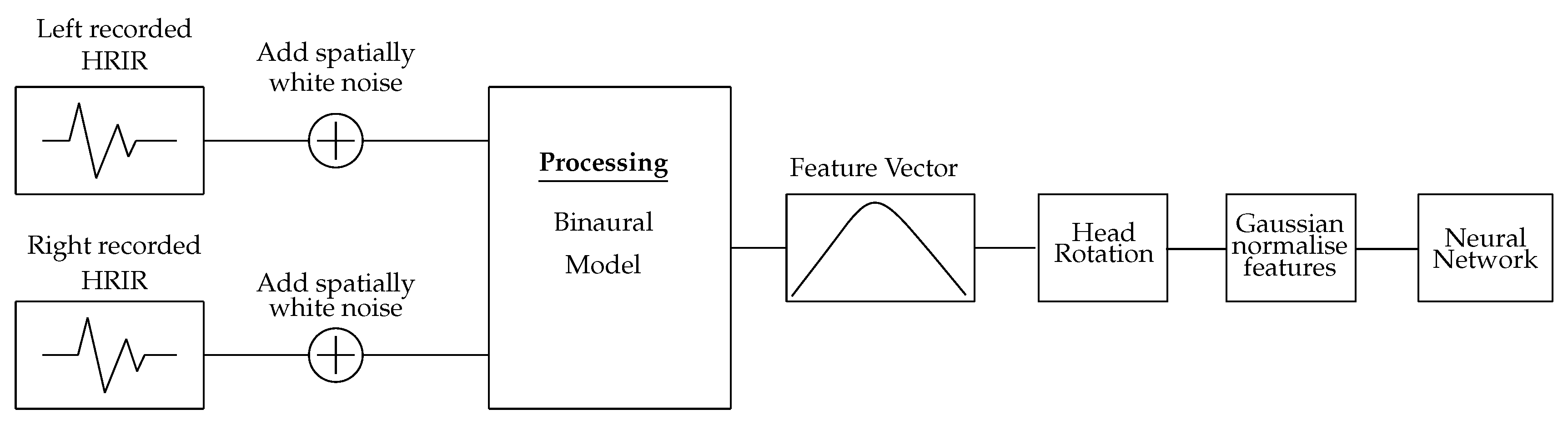
The binaural model presented in Section 2.1 is used to generate a training feature matrix using the un-compensated ‘raw’ SADIE KEMAR dataset [23]. This dataset contains an HRIR grid of 1550 points: 5° increments across the azimuth in steps of 10° elevation. To train the NN, only the HRIRs relating to 0° elevation were used, providing a dataset of 104 HRIRs. A multi-conditional training (MCT) dataset is created by adding spatially white noise to the HRIRs at 0 dB, 10 dB and 20 dB signal-to-noise ratios. This spatially white noise is generated by convolving Gaussian white noise with all 1550 HRIRs in the SADIE KEMAR dataset and averaging the resulting localised noise across the 1550 positions; producing a spatially white noise signal matrix [15]. This addition of spatially white noise is based on the findings in [9,10,15], which found that training the NN with data under different noise conditions improved generalisation. These HRIRs with added spatially white noise are then analysed by the binaural model and the output used to create the feature vector. The neural network is only trained using these HRIRs with noise mixtures, and no reflected components of BRIRs are included as part of the training data
Two training matrices are created by concatenating the feature vector of one HRIR with the feature vector produced by an HRIR corresponding to either a ° or ° rotation of KEMAR with the same signal-to-noise ratio. This produces two feature matrices with which two neural networks can be trained with, one for each rotation. The use of an NN for each fixed rotation angle was found to produce more accurate results than having one NN trained for both.
The use of ‘head rotation’ has a biological precedence, in that humans use head rotation to focus on the location of a sound source; disambiguating front-back confusions that occur due to interaural cue similarities between signals arriving from opposing locations in the front and back hemispheres [6,20]. In this study, the equivalent effect of implementing a head rotation is realised by taking the impulse response measurements at two additional fixed measurement orientations (at ±90°). The use of fixed rotations reduces the number of additional signals needed to train the NN and reduces the number of additional measurements that need to be recorded. The use of additional measurement positions corresponding to receiver rotations of ° was found to produce lower maximum errors when compared to rotations of °, ° and ° (Table 1). The two training matrices are used to train two NN, one for each rotation, and the network trained with the ° rotation dataset is used to predict the DoA for signals that originate on the left hemisphere, while the ° NN is used to predict the DoA for signals on the right hemisphere. Each of these NNs is trained with the full azimuth range to allow the NNs to predict the DoA for signals with ambiguous feature vectors that may be classified as originating from the wrong hemisphere. When testing the NN, the additional measurement positions are assigned to the signals based on the location of the maximum peak in the IACC feature vector. If the peak index in the IACC is less than 50 (signal originated in the left hemisphere), a receiver rotation of ° is applied; otherwise, a receiver rotation of ° is used. To normalise the numeric values, the training data were Gaussian-normalised to ensure each feature had zero mean and unit variance. The processing workflow for the training data can be seen in Figure 2.
2.3. Neural Network
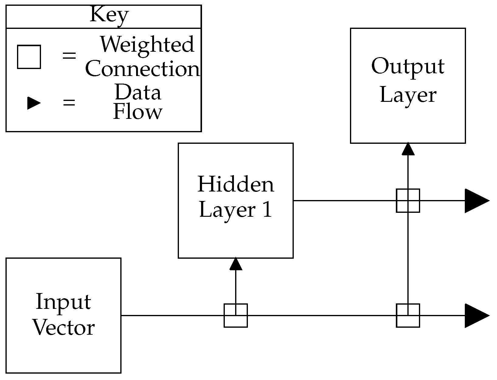
TensorFlow [24], a commonly-used python library designed for the development and execution of machine learning algorithms, is used to implement a cascade-correlation NN, the topology of which connects the input feature vector to every layer within the NN. Additionally, all layers’ outputs are connected to subsequent layers in the NN, as in Figure 3 [25]. The use of NN over GMM was chosen based on findings in [15], which suggested that DNN outperformed GMM for binaural localisation tasks. The decision to use the cascade-correlation NN was based on comparisons between the cascade-correlation NN architecture and the MLP, which showed that the cascade-correlation NN arrived at a more accurate solution with less training required compared to the MLP (Table 2).
The NN consists of an input layer, one hidden layer and an output layer. The input layer contains one node for each feature in the training data; the hidden layer contains 128 neurons each with a hyperbolic tangent activation function; and the output layer contains 360 neurons, one for each azimuth direction from 0° to 359°. Using 360 output neurons as opposed to 104 (one for each angle of the training dataset) allows the NN to make attempts at predicting the DoA for both known and unknown source positions. A softmax activation function is then applied to the output layer of the NN, producing a probability vector predicting the likelihood of the analysed signal having arrived from each of the 360 possible DoAs.
Each data point, whether it be a feature in the input feature vector or the output of a previous layer, is connected to a neuron via a weighted connection. The summed response of all the weighted connections linked to a neuron defines that neuron’s level of activation when presented with a specific data configuration, a bias is then applied to this activation level. These weights and biases for each layer of the NN are initialised with random values, with the weights distributed such that they will be zero mean and have a standard deviation () defined as:
where m is the number of inputs to hidden layer i [26].
The NN is trained over a maximum of 600 epochs, with the training terminating once the NN reached 100% accuracy or improvement saturation. Improvement saturation is defined as no improvement over a training period equal to of the total number of epochs. Mini-batches are used to train the NN with sizes equal to of the training data. The order of the training data is randomised after each epoch, so the NN never receives the same batch of data twice. The adaptive moment estimation (ADAM) optimiser [27] is used for training, using a learning rate of 0.001, a value of 0.9, a value of 0.99 and an value of . The values define the exponential decay for the moment estimates, and is the numerical stability constant [27].
The NN’s targets are defined as a vector of size 360, with a one in the index relating to the DoA and all other entries equal to zero. The DoA is therefore extracted from the probability vector produced by the NN as the angle with the highest probability such that,
where represents the probability of azimuth angle given the feature vector x. The probability is calculated as,
where w denotes a set of weights, is the output biases and is the output from the hidden layer calculated as,
2.4. Testing Methodology
A key measure of the success of an NN is its ability to generalise across different datasets other than that with which it was trained. To test the generalisability of the proposed NN, a dataset was produced in an anechoic chamber for both a KEMAR 45BC [17] and Neumann KU100 [28] binaural dummy head, using an Equator D5 coaxial loudspeaker [29]. The exponential sine sweep method [30] was used to generate the BRIRs, with a swept frequency range of 20 Hz to 22 kHz over ten seconds. To be able to test the NN’s performance at predicting the DoA of reflections, a flat wooden reflective surface mounted on a stand was placed in the anechoic chamber, such that a reflection with a known DoA would be produced (Figure 4). This allows for the accuracy of the NN at predicting the DoA for a reflected signal to be tested, without the presence of overlapping reflections that could occur in non-controlled environments. To approximate an omnidirectional sound source, the BRIRs were averaged over four speaker rotations (0°, 90°, 180° and 270°); omnidirectional sources are often desired in impulse response measurements for acoustic analysis [31], as they produce approximately equal acoustic excitation throughout the room. The extent to which this averaged loudspeaker response will be omnidirectional will vary across different loudspeakers, particularly at higher frequencies where loudspeakers tend to be more directional. Averaging the response of the room over speaker rotations does result in some spectral variation, particularly with noisier signals; however, this workflow is similar to that employed when measuring the impulse response of a room.
To calculate the required location of the reflective surface such that a known DoA would be produced, a simple MATLAB image source model based on [32] was used to calculate a point of incidence on a wall that would produce a first order reflection in a 3 m × 3 m × 3 m room with the receiver positioned in the centre of the room. The reflective surface was then placed in the anechoic chamber based on the angle of arrival and distance between the receiver and calculated point of incidence. Although care was taken to ensure accurate positioning of the individual parts of the system, it is prone to misalignments due to the floating floor in the anechoic chamber, which can lead to DoAs that differ from that which is expected.
With these BRIRs only having two sources of impulsive sounds, the direct sound and first reflection, a simple method for separating these signals was employed. Firstly, the maximum absolute peak in the signal is detected and assumed to belong to the direct sound. A 170 sample frame around the peak location indexed at was used to separate the direct sound from the signal. It was ensured that all segmented audio samples only contained audio pertaining to the direct sound. The process was then run again to detect the location of the reflected component, and each segment was checked to ensure only audio pertaining to the reflected component was present (see Figure 5 for an example BRIR with window locations). When dealing with BRIRs measured in less controlled environments, a method for systematically detecting discrete reflections in the BRIR is required, and various methods have been proposed in the literature to detect reflections in impulse responses, including [4,33,34,35].
The separated signals were then analysed using the binaural model and a test data matrix generated by combining the segmented direct or reflected component with the corresponding rotated signal (as described in Section 2.2). The positively and negatively rotated test feature vectors were stored in separate matrices and used to test the NN trained with the corresponding rotation dataset (as described in Section 2.2). The data was then Gaussian normalised across each feature in the feature vector, using the mean and standard deviations calculated from the training data.
The generated test data consisted of 144 of these BRIRs, with source positions from 0° to 357.5° and reflections from 1° to 358.5° using a turntable to rotate the binaural dummy head in steps of 2.5° (with the angles rounded for comparison with the NN’s output). This provided 288 angles with which to test the NN: 144 direct sounds and 144 reflections. The turntable was covered in acoustic foam to attempt to eliminate any reflections that it would produce.
3. Results
The two NNs trained with the SADIE HRIR dataset (as described in Section 2.1 and Section 2.2) were tested with the components of the measured test BRIRs (as described in Section 2.4), with the outputs concatenated to produce the resulting direction of arrival for the direct and reflected components. The angular error was then computed as the difference between the NN predictions and the target values. The training of the neural network generally terminated due to saturation in output performance within 122 epochs, with an accuracy of 95% and a maximum error of 5°. Statistical analysis of the prediction errors was performed using MATLAB’s one-way analysis of variance (ANOVA) function [36] and is reported in the format: ANOVA(F(between group degrees of freedom, within groups degree of freedom) = F value, p = significance), all of these values are returned by the anova1 function [36].
A baseline method used as a reference to compare results obtained from the NN can be derived from the ITD equation (Equation (8) taken from [37]) rearranged for calculating the DoA,
where d is the distance between the two ears, is the DoA, and c is the speed of sound [37]. The ITD value used for the baseline DoA predictions was measured by locating the maximum peak in the IACC feature vector, as calculated using the binaural model proposed in Section 2.1. The index for this peak in the IACC feature vector relates to one of 99 ITD values linearly spaced from −1.1 ms to 1.1 ms.
In Table 3, the neural network accuracy across the test data is presented. The results show that for the direct sound, the neural network predicted 64.58% and 68.06% of the DoAs within 5° for the KEMAR and KU100 dummy head, respectively. Although when analysing direct sound captured with the KU100, a greater percentage of predictions are within ° of the target value, the neural network makes a greater number of exact predictions and has lower relative error for KEMAR. This observation is expected given the different morpho-acoustic properties of each head and their ears, which could lead to differences in the observed interaural cues, particularly those dependent on spectral information. The results show that the neural network performs worse when analysing the reflected components. In this case, the reflected component measured with the KU100 is more accurately localised, with lower maximum error, relative error, root mean squared error and number of front-back confusions. Comparisons between the accuracy of the proposed method with the baseline shows that the NN is capable of reaching a higher degree of accuracy, with lower angular error and fewer front-back confusions.
In Figure 6, comparisons between the direct sound and reflected component for BRIRs captured with the KEMAR 45BC are presented. The boxplots show that for the direct sound, a maximum error of 12° and median error of 5° (mean error of 4.20°) were observed, while the reflected component has a maximum error of 30° and median of 8.5° (mean error of 10.87°). There is a significant difference in the neural network performance between the direct sound and reflected component, ANOVA(F(1,286) = 83.99, p < 0.01). This observed difference could result from the difference in signal path distance, which was found to reduce prediction accuracy in [9,10]. May et al. reported that as source-receiver distances increased, and therefore the signal level relative to the noise floor or room reverberation decreased, the accuracy of the GMM predictions decreased. They reported that, averaged over seven reverb times, the number of anomalous predictions made by the GMM increased by 9% between a source-receiver distance of 2 m compared to a source-receiver distance of 1 m. Further causes of error could be due to system misalignment at point of measurement or lower signal-to-noise ratios (SNR) occurring due to signal absorption at the reflector and larger propagation path (source-reflector-receiver); an average SNR of approximately 22.40 dB and 13.14 dB was observed across the direct and reflected component, respectively.
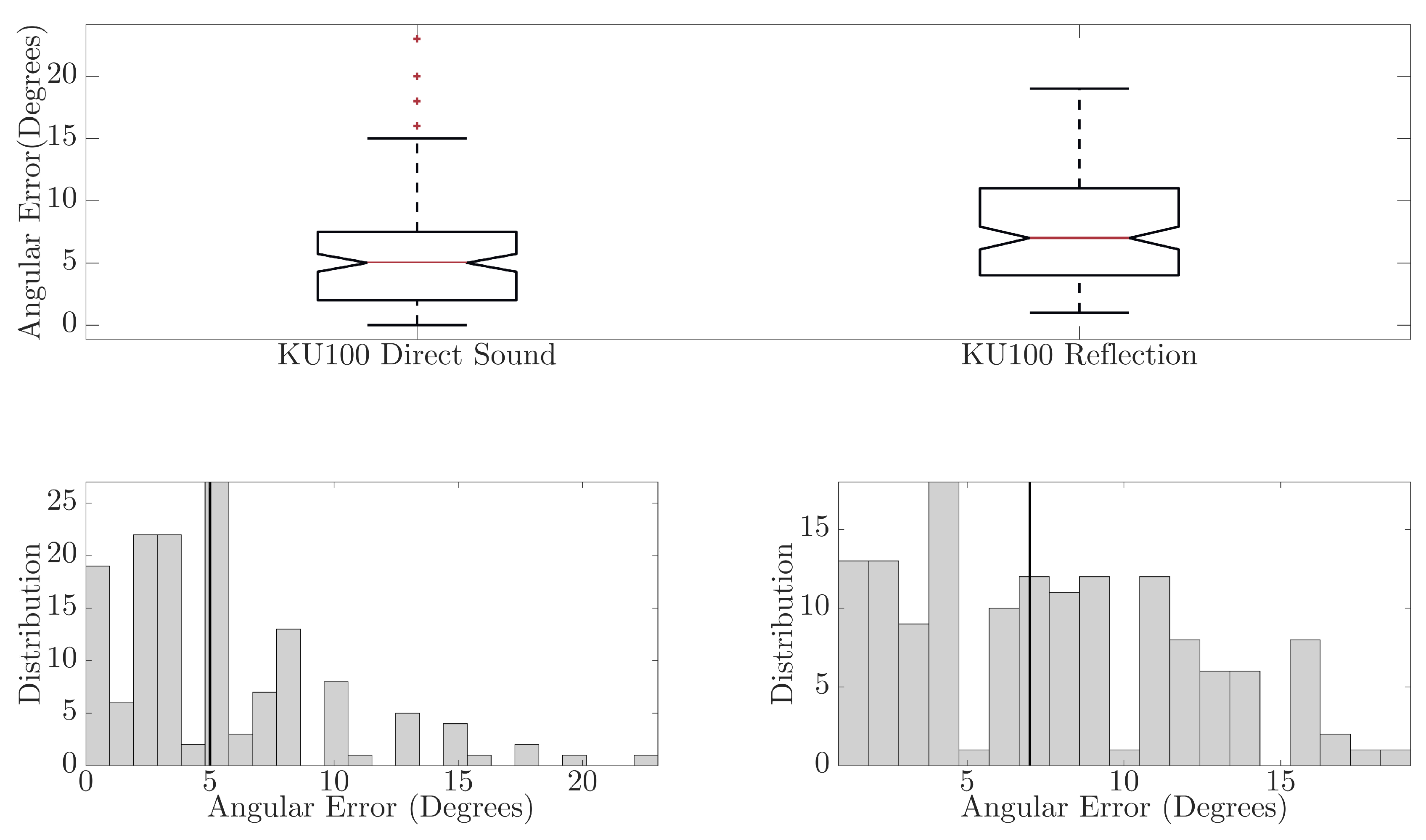
In Figure 7, the comparison between direct sound and reflected component for BRIRs captured using the KU100 are presented. The boxplots show that for the direct sound, a maximum error of 23° is observed and a median error of 5° (mean error of 5.15°), and the reflected component had a maximum error of 19° and median of 7° (mean error of 7.51°). Although the maximum and median errors are not too dissimilar between the predictions for the direct sound and reflected component, there is a significant difference in the distribution of the angular errors, ANOVA(F(1,286) = 18.85, p < 0.01). The direct sound DoA predictions are generally more accurate than those for the reflected component. As with the findings for the KEMAR, this could be due to the difference in signal paths between the direct sound and reflected component, system misalignment or lower SNR; an average SNR of approximately 22.41 dB and 10.91 dB was observed across direct sound and reflected components, respectively.
In Figure 8, the comparison between the two binaural dummy heads is presented for both the direct sound and reflected components of the BRIRs. The box plots show that there is no significant difference between the medians for the direct sound, and while the maximum error observed for DoA predictions with the KU100 is higher than that of the KEMAR, there is no significant difference in the angular errors between the two binaural dummy heads, ANOVA(F(1,286) = 4.29, p = 0.04). This would suggest that for at least the direct sound, the NN is generalisable to new data, including those which are produced using a different binaural dummy head microphone from those which were used to train the NN. However, comparing the angular errors observed in the output of the NN for the reflected component shows that the KU100 has a significantly lower median angular error and performs significantly better overall when analysing the reflected components captured with the KU100, ANOVA(F(1,286) = 18.23, p < 0.01). This observation does not match what would be expected given that the NN was trained with HRIRs captured using a KEMAR unit, suggesting that the NN should perform better or comparably when predicting the DoA for reflected signals captured using another KEMAR over the results obtained with the KU100.
Figure 6 and Figure 7 compare the accuracy of the NN predictions for direct and reflected components for each head. The difference between the direct sound and reflected component is more dissimilar for BRIRs captured with the KEMAR than the KU100, possibly suggesting the presence of an external factor that is creating ambiguity in the measured binaural cues for the reflected components captured using the KEMAR. Furthermore, comparing the interaural cues (Figure 9 and Figure 10) between the direct sound and reflected components of the BRIR for the KEMAR and KU100 measurements shows a more distinct blurring for the reflected components measured with the KEMAR when compared to those measured with the KU100. This could suggest that a source of interference is present in the KEMAR measurements that is producing ambiguity in the measured signals’ interaural cues. This could be due to noise present within the system and environment or misalignment in the measurement system for the KEMAR measurements; leading to the production of erroneous reflected signals.
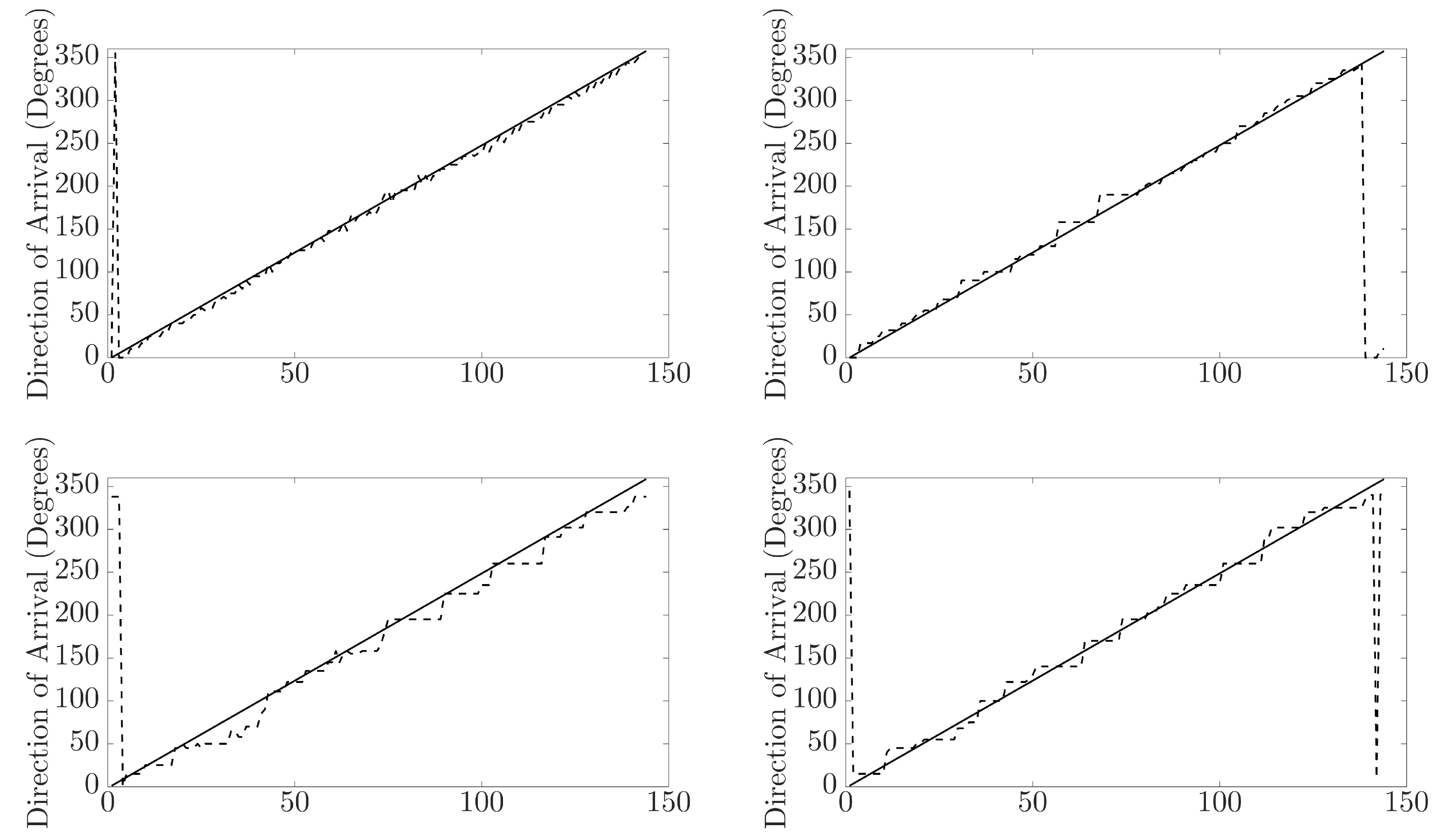
By investigating the neural networks’ predicted direction of arrival compared against the expected, insight can be gained into any patterns occurring in the NN output predictions. Additionally, it will show how capable the NN is at predicting the DoA for signals with a DoA not represented within the training data. In Figure 11, the predicted direction of arrival by the neural network (dashed line) is compared against the expected direction of arrival (solid line), and the plot shows the comparison for the KEMAR direct sound measurement predictions (top left), KEMAR reflection measurement predictions (bottom left), KU100 direct sound measurement predictions (top right) and KU100 reflection measurement predictions (bottom right). Generally, the direct sound measurement predictions are mapped to the closest matching DoA represented in the training database, suggesting that the NN is incapable of making predictions for untrained directions of arrival. In the case of the reflections, the NN predictions tend to plateau over a larger range of expected azimuth DoA. This observation further shows the impact of the blurring of the interaural cues (Figure 9 and Figure 10) producing regions of ambiguous cues in the reflection measurements, causing the NN to produces regions of the same DoA prediction.
4. Discussion
The results presented in Section 3 show that there is no significant difference in the accuracy of the NN when analysing the direct sound of BRIRs captured with both the KEMAR 45BC and the KU100. However, the accuracy of the NN is significantly reduced when analysing the reflected component of the BRIRs, with the NN performing better at predicting the DoA of reflected components measured with the KU100. A reduction in performance would be expected between the direct sound and reflected component, due to the lower signal-to-noise ratio that would be observed for the reflected component. It is of interest that reflections measured with the KU100 are more accurately localised than those measured with the KEMAR 45BC; this could be due to a greater degree of system misalignment in the KEMAR 45BC measurements that was not present in the KU100 measurements. An additional difference that could lead to more accurate predictions being made for the KU100 could be the diffuse-field flat frequency response of the KU100, which could produce more consistent spectral cues for the reflected component (as seen in Figure 10), leading to more accurate direction of arrival predictions by the neural network.
Analysis over different degrees of measurement orientation rotations (Table 1) showed that while the number of predictions within ° varies little between degrees of rotation, the maximum error in the neural networks’ prediction decreases as the angle of rotation increases. Larger degrees of rotation would produce greater differences in interaural cues between the rotated and original signal, allowing the neural network to produce more accurate predictions under noisier conditions where the interaural cues become blurred. The use of additional measurement orientations decreases the number of front-back confusions, with generally larger degrees of receiver rotations producing fewer front-back hemisphere errors, except when using °. Using larger degrees of rotation has the additional benefit of reducing the maximum predictions errors made by the neural network; this could be due to the greater rotational mobility allowing signals at the rear of the listener to be focused more in the frontal hemisphere; producing more accurate direction of arrival predictions. It is interesting that there is a greater percentage of front-back confusions for the KEMAR 45BC compared to the KU100; this could be due to differences in system alignment causing positions close to 90° and 270° (source facing the left or right ear) to originate from the opposite hemisphere.
The lack of significant difference between the direct sounds measured with the two binaural dummy heads agrees with the findings of May et al. [11], who found that a GMM trained with an MCT dataset was able to localise sounds captured with two different binaural dummy heads. The notable difference between the KEMAR 45BC and KU100 include: morphological differences of the head and ears between binaural dummy head microphones; the KEMAR 45BC has a torso; the KU100’s microphones have a flat diffuse-field frequency response; and the material used for the dummy head microphones.
The overall accuracy of the method presented in this paper is, however, lower than that found in [11]. This could be a result of the type of signals being analysed, which, in this study, are 3.8 ms-long impulsive signals as opposed to longer speech samples. Compared to more recent NN-based algorithms [15], the proposed algorithm under performs compared to reported findings of 83.8% to 100% accuracy across different test scenarios. However, their analyses only considered signals in the frontal hemisphere around the head and considered longer audio samples for the localisation problem.
Comparing the proposed method to that presented in [12] shows that the proposed method achieves lower relative errors for the direct sound and reflections measured with both binaural dummy head microphones, compared to the 24.0% reported for real test sources using a multi-layered perceptron in [12].
The average errors reported in this paper are lower than that presented in [4], which reported average errors in the range of 28.7° and 54.4° when analysing the components of measured BRIRs. However, the results presented in [4] considered reflections with reflection orders greater than first, and therefore, further analyses of the proposed NNs’ performance with full BRIRs is required for more direct comparisons to be made.
Future work will focus on improving the accuracy of the model for azimuth DoA estimation, using measured binaural room impulse responses to assess the accuracy of the neural network as reflection order and propagation path distance increases. The proposed model will then be extended on to consider estimation of elevation DoA, providing complete directional analysis of the binaural room impulse responses; the aim being for the final method to be integrated within a geometry inference and reflection backpropagation algorithm, allowing for in-depth analysis of the acoustics of a room. However, this will require higher accuracy in the DoA predictions for the reflections. Further avenues of research to improve the robustness of the algorithm could include: the use of noise reduction techniques to ideally reduce the ambiguity in the binaural cues, increasing the size of the training database used to train the neural network, investigation into using different representations of interaural cues and how they are extracted from the signals, using reflections to train the NN in addition to the HRIRs or the use of a different machine learning classifier.
5. Conclusions
The aim of this study was to investigate the application of neural networks in the spatial analysis of binaural room impulse responses. The neural network was tested using binaural room impulse responses captured using two different binaural dummy heads. The neural network was shown to have no significant difference in accuracy when analysing the direct sound of the binaural room impulse response across the two binaural dummy heads, with 64.58% and 68.06% of the predictions being within ° of the expected values for KEMAR and the KU100, respectively. However, upon presenting the NN with reflected components for analysis, the accuracy of the predictions was significantly reduced. The NN also generally produces more accurate results for reflected components of the binaural room impulse response captured with the KU100. Comparisons of the interaural cues for the direct sound and reflected components show a distinct blurring in the cues for the reflected components measured with KEMAR, which is present to a lesser extent for the KU100. This blurring could be a product of lower signal-to-noise ratios or misalignment in the measurement systems, leading to greater ambiguity in the measurements. The results presented in this paper show the potential of using this technique as a tool for analysing binaural room impulse responses, while indicating that further work is required to improve the robustness of the algorithm for analysing reflections and signals with lower signal-to-noise ratios. Further development of this algorithm will investigate the application of the neural network for elevation direction of arrival analysis and integration of the method with geometry inference and reflection back-propagation algorithms, allowing for analysis of a room’s geometry and its affect on sounds played within it.
Acknowledgments
Funding was provided by a UK Engineering and Physical Sciences Research Council (EPSRC) Doctoral Training Award, the Department of Electronic Engineering at the University of York, and in part by Digital Creativity Labs, EPSRC Grant Number: EP/M023265/1.
Author Contributions
Michael Lovedee-Turner developed the concepts, algorithms and experiments and wrote the paper. Damian Murphy supervised the project and paper writing, providing input throughout the development process.
Conflicts of Interest
The authors declare no conflict of interest
Abbreviations
The following abbreviations are used in this manuscript:
| DoA | Direction of arrival |
| ITD | Interaural time difference |
| ILD | Interaural level difference |
| HRIR | Head-related impulse responses |
| NN | Neural network |
| DNN | Deep neural networks |
| GMM | Gaussian mixture model |
| IACC | Interaural cross-correlation |
| FFT | Fast Fourier transform |
| MCT | Multi-conditional training |
| ADAM | Adaptive moment estimation |
| BRIR | Binaural room impulse responses |
| SNR | Signal-to-noise ratio |
| ANOVA | Analysis of variance |
References
- Pulkki, V.; Merimaa, J. Spatial impulse response rendering II: Reproduction of diffuse sound and listening tests. J. Audio Eng. Soc. 2006, 54, 3–20. [Google Scholar]
- Pulkki, V. Spatial sound reproduction with directional audio coding. J. Audio Eng. Soc. 2007, 55, 503–516. [Google Scholar]
- Tervo, S.; Pätynen, J.; Lokki, T. Acoustic reflection path tracing using a highly directional loudspeaker. In Proceedings of the IEEE Workshop on Applications of Signal Processing to Audio and Acoustics, New Paltz, NY, USA, 18–21 October 2009; pp. 245–248. [Google Scholar]
- Vesa, S.; Lokki, T. Segmentation and Analysis of Early Reflections From a Binaural Room Impulse Response; Technical report; Helsinki University of Technology: Helsinki, Finland, 2009. [Google Scholar]
- Kohlrausch, A.; Braasch, J.; Kolosssa, D.; Blauert, J. An introduction to binaural processing. In The Technology of Binaural Listening; Blauert, J., Ed.; Springer-Verlag: Berlin/Heidelberg, Germany, 2013; pp. 1–32. [Google Scholar]
- Howard, D.; Angus, J. Acoustics and Psychoacoustics, 4th ed.; Elsevier Science: Cambridge, UK, 2009. [Google Scholar]
- Zhong, X. Localize a sound source in self motion with ITD Cues. In Dynamic Spatial Hearing by Human and Robot Listeners; Arizona State University: Tempe, AS, USA, 2015; pp. 52–68. [Google Scholar]
- Musicant, A.D.; Butler, R.A. The influence of pinnae-based spectral cues on sound localization. J. Acoust. Soc. Am. 1984, 75, 1195–1200. [Google Scholar] [CrossRef] [PubMed]
- May, T.; Van De Par, S.; Kohlrausch, A. A probabilistic model for robust localization based on a binaural auditory front-end. IEEE Trans. Audio Speech Lang. Process. 2011, 19, 1–13. [Google Scholar] [CrossRef]
- Woodruff, J.; Wang, D. Binaural localization of multiple sources in reverberant and noisy environments. IEEE Trans. Acoust. Speech Signal Process. 2012, 20, 1503–1512. [Google Scholar] [CrossRef]
- May, T.; Ma, N.; Brown, G.J. Robust localisation of multiple speakers exploiting head movements and multi-conditional training of binaural cues. In Proceedings of the IEEE International Conference on Acoustics, Speech and Signal Processing (ICASSP), Brisbane, Australia, 19–24 April 2015; pp. 2679–2683. [Google Scholar]
- Palomäki, K.; Pulkki, V.; Karjalainen, M. Neural network approach to analyze spatial sound. In Proceedings of the AES 16th International Conference: Spatial Sound Reproduction, Rovaniemi, Finland, 10–12 April 1999; pp. 233–245. [Google Scholar]
- Backman, J.; Karjalainen, M. Modelling of human directional and spatial hearing using neural networks. In Proceedings of the IEEE International Conference on Acoustics, Speech, and Signal Processing, Minneapolis, MN, USA, 27–30 April 1993; pp. I-125–I-128. [Google Scholar]
- Yuhas, B.P. Automated Sound Localization Through Adaptation. In Proceedings of the International Joint Conference on Neural Networks (IJCNN), Baltimore, MD, USA, 7–11 June 1992; pp. II-907–II-912. [Google Scholar]
- Ma, N.; Brown, G.J.; May, T. Exploiting deep neural networks and head movements for binaural localisation of multiple speakers in reverberant conditions. In Interspeech; International Speech Communication Association: Baixas, France, 2015; pp. 1–5. [Google Scholar]
- Ding, J.; Wang, J.; Zheng, C.; Peng, R.; Li, X. Analysis of Binaural Features for Supervised Localization in Reverberant Environments. In Proceedings of Audio Engineering Society Convention 141; Audio Engineering Society: Los Angeles, CA, USA, 2016; pp. 1–9. [Google Scholar]
- GRAS. KEMAR Model 45BC. 2016. Available online: http://www.gras.dk/45bc.html (accessed on 25 October 2016).
- Pulkki, V.; Karjalainen, M.; Huopaniemi, J. Analyzing Virtual Sound Source Attributes Using Binaural Auditory Model. J. Audio Eng. Soc. 1999, 47, 203–217. [Google Scholar]
- Woodruff, J.; Wang, D. Sequential organization of speech in reverberant environments by integrating monaural grouping and binaural localization. IEEE Trans. Audio Speech Lang. Process. 2010, 18, 1856–1866. [Google Scholar] [CrossRef]
- Middlebrooks, J.C.; Green, D.M. Sound Localization By Human Listeners. Ann. Rev. Pyschol. 1991, 42, 135–159. [Google Scholar] [CrossRef] [PubMed]
- Slaney, M. Auditory Toolbox. 1998. Available online: https://engineering.purdue.edu/~malcolm/interval/1998-010/ (accessed on 28 December 2017).
- Gao, B. Cochleagram and IS-NMF2D for Blind Source Separation. 2014. Available online: http://uk.mathworks.com/matlabcentral/fileexchange/48622-cochleagram-and-is-nmf2d-for-blind-source-separation?focused=3855900&tab=function (accessed on 28 December 2017).
- Kearney, G. SADIE Binaural Measurements. 2016. Available online: http://www.york.ac.uk/sadie-project/binaural.html (accessed on 28 December 2017).
- Google. TensorFlow. Available online: https://www.tensorflow.org/ (accessed on 28 December 2017).
- Fahlman, S.E.; Lebiere, C. The Cascade-Correlation Learning Architecture. In Advances in Neural Information Processing Systems 2; Morgan Kaufmann Publishers Inc.: San Francisco, CA, USA, 1990; pp. 524–532. [Google Scholar]
- LeCun, Y.A.; Bottou, L.; Orr, G.B.; Müller, K.R. Efficient BackProp. In Neural Networks: Tricks of the Trade; Springer: Berlin/Heidelberg, Germany, 1998; pp. 9–50. [Google Scholar]
- Kingma, D.; Ba, J. Adam: A method for stochastic optimization. In Proceedings of the International Conference on Learning Representations, San Diego, CA, USA, 7–9 May 2015; pp. 1–15. [Google Scholar]
- Neumann. Dummy Head KU100. Available online: https://www.neumann.com/?lang=en&id=current_microphones&cid=ku100_description (accessed on 28 December 2017).
- Equator Audio. Equator D5 Coaxial Loudpseakers. Available online: http://www.equatoraudio.com/New-Improved-D5-Studio-Monitors-Pair-p/d5.htm (accessed on 28 November 2017).
- Farina, A. Simultaneous measurement of impulse response and distortion with a swept-sine technique. In Proceedings of the108th Convention, Paris, France, 19–22 February 2000; pp. 1–15. [Google Scholar]
- British Standards Institution. BSI Standard ISO 3382-1: Acoustics—Measurements of Room Acoustic Parameters Part 1: Performance Spaces (ISO 3382-1:2009). 2009. Available online: https://www.iso.org/standard/40979.html (accessed on 5 January 2018).
- Allen, J.B. Image method for efficiently simulating small-room acoustics. J. Acoust. Soc. Am. 1979, 65, 943. [Google Scholar] [CrossRef]
- Kelly, I.; Boland, F. Detecting Arrivals in Room Impulse Responses with Dynamic Time Warping. IEEE/ACM Trans. Audio Speech Lang. Process. 2013, 22, 1139–1147. [Google Scholar] [CrossRef]
- Remaggi, L.; Jackson, P.J.B.; Coleman, P.; Wang, W. Acoustic Reflector Localization: Novel Image Source Reversion and Direct Localization Methods. IEEE/ACM Trans. Audio Speech Lang. Process. 2017, 25, 296–309. [Google Scholar] [CrossRef]
- Defrance, G.; Daudet, L.; Polack, J.D. Detecting arrivals within room impulse responses using matching pursuit. In Proceedings of the 11th International Conference on Digital Audio Effects (DAFx-08), Espoo, Finland, 1–4 September 2008; pp. 1–4. [Google Scholar]
- MATLAB. Anova1. 2017. Available online: https://uk.mathworks.com/help/stats/anova1.html (accessed on 28 December 2017).
- Howard, D.; Angus, J. Interaural time difference. In Acoustics and Psychoacoustics, 2nd ed.; Focal Press: Oxford, UK, 2001. [Google Scholar]
Figure 1.
Example of the interaural cross-correlation function (top) and interaural level difference (bottom) for a HRIR with a source positioned at azimuth = 90° and elevation = 0°.
Figure 1.
Example of the interaural cross-correlation function (top) and interaural level difference (bottom) for a HRIR with a source positioned at azimuth = 90° and elevation = 0°.
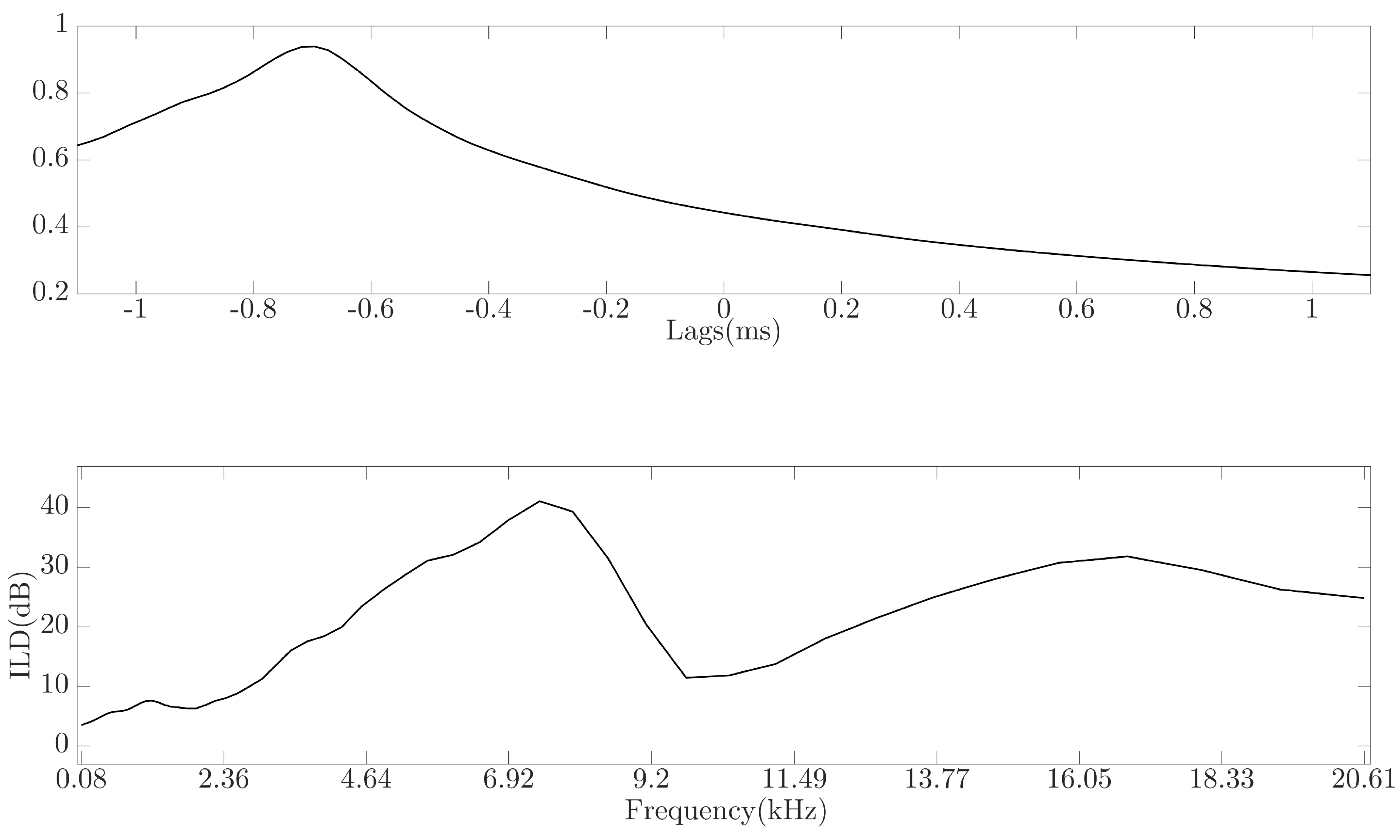
Figure 2.
Signal processing chain used to generate the training data used to train the neural network.
Figure 2.
Signal processing chain used to generate the training data used to train the neural network.

Figure 3.
Cascade-correlation neural network topology used, where triangles signify the data flow and squares are weighted connections between the hidden layers and the incoming data.
Figure 3.
Cascade-correlation neural network topology used, where triangles signify the data flow and squares are weighted connections between the hidden layers and the incoming data.

Figure 4.
Measurement setup showing the reflective surface (A), KEMAR 45BC (B) and Equator D5 Coaxial Loudspeaker (C).
Figure 4.
Measurement setup showing the reflective surface (A), KEMAR 45BC (B) and Equator D5 Coaxial Loudspeaker (C).
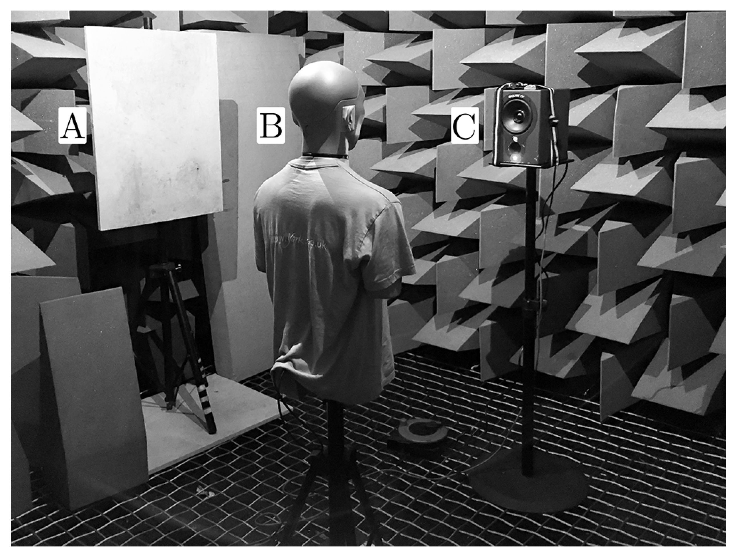
Figure 5.
Example binaural room impulse response generated with source at azimuth = 0° and reflector at azimuth = 71°; the solid line is the left channel of the impulse response; the dotted line is the right channel of the impulse response; and the windowed area denotes the segmented regions using the technique discussed in Section 2.4.
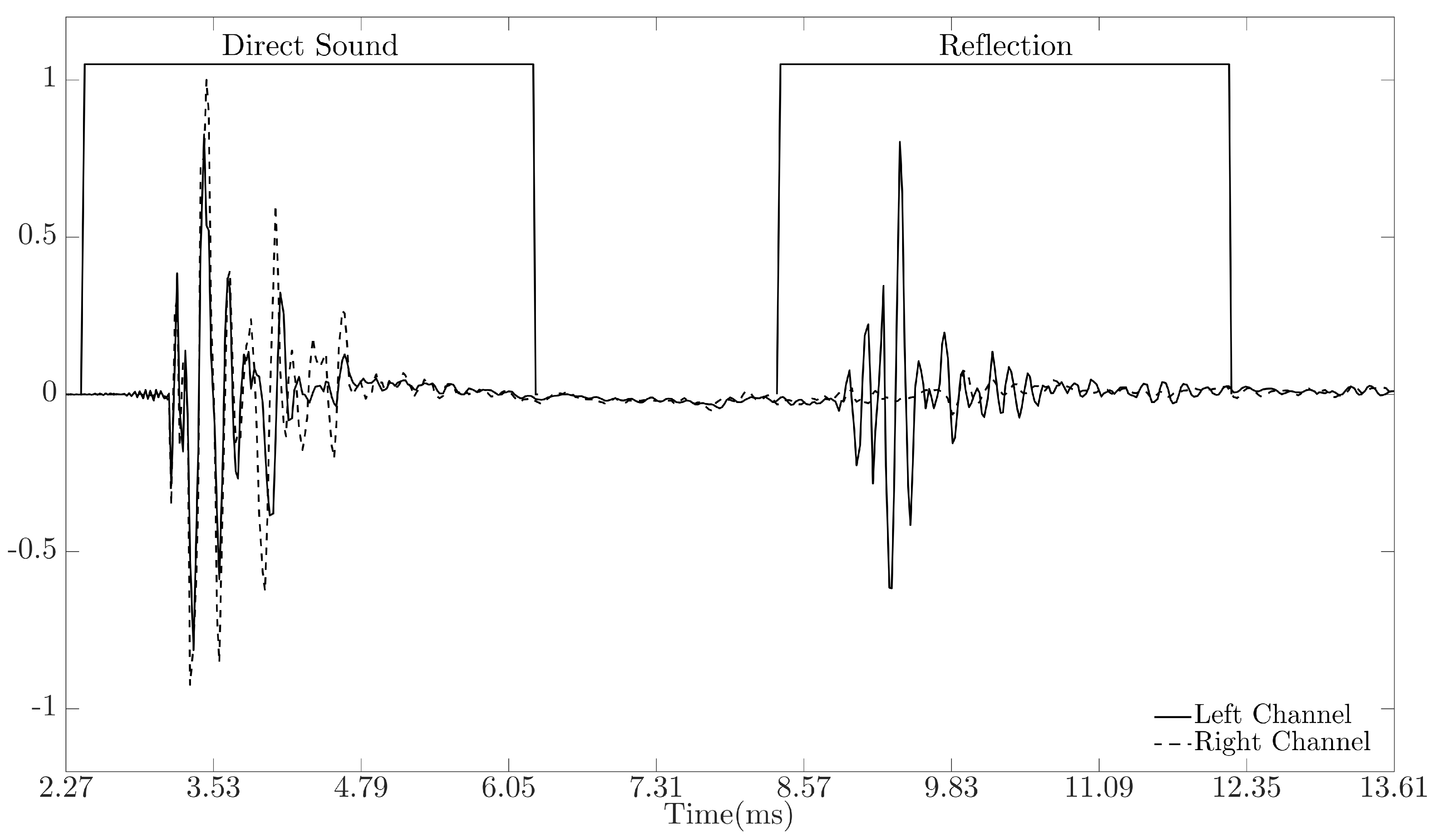
Figure 6.
Comparison of angular errors in the neural network direction of arrival predictions for measurements with the KEMAR 45BC. The top image is a boxplot comparison of the angular error in the neural network predictions for the direct sound and reflected components. The bottom left is a histogram showing the error distribution for the direction of arrival predictions of the direct sound, and the bottom right is the error distribution for the direction of arrival predictions of the reflected components. The black line on the histograms depicts the median angular error.
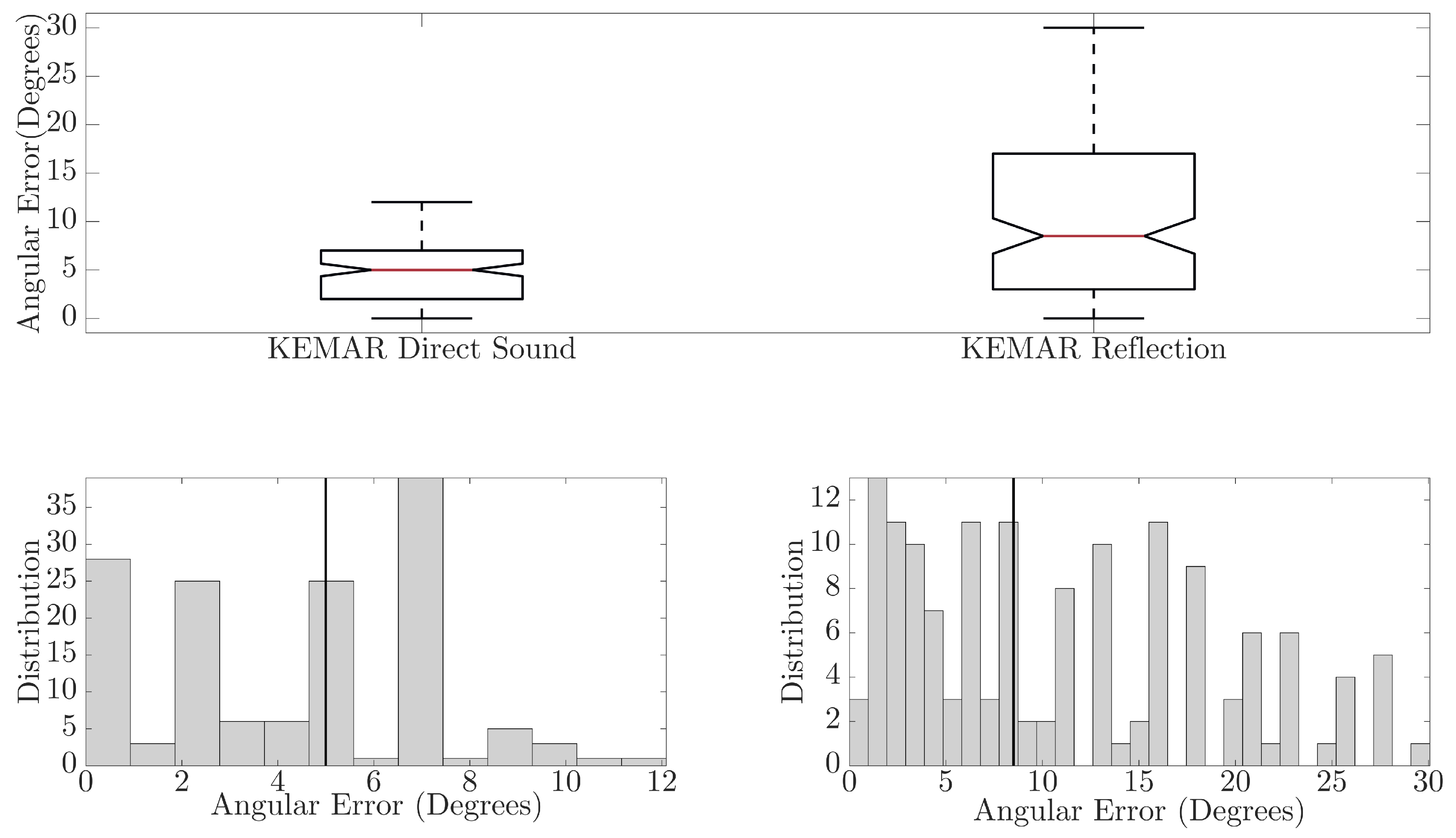
Figure 7.
Comparison of angular errors in the neural network direction of arrival predictions for measurements with the KU100. The top image is a boxplot comparison of the angular error in the neural network predictions for the direct sound and reflected components; the bottom left is a histogram showing the error distribution for the direction of arrival predictions of the direct sound; and the bottom right is the error distribution for the direction of arrival predictions of the reflected components. The black line on the histograms depicts the median angular error.

Figure 8.
Boxplot comparison of angular errors in the neural network direction of arrival predictions between the KEMAR and KU100 dummy heads for direct sound (top) and reflected (bottom) components.
Figure 8.
Boxplot comparison of angular errors in the neural network direction of arrival predictions between the KEMAR and KU100 dummy heads for direct sound (top) and reflected (bottom) components.
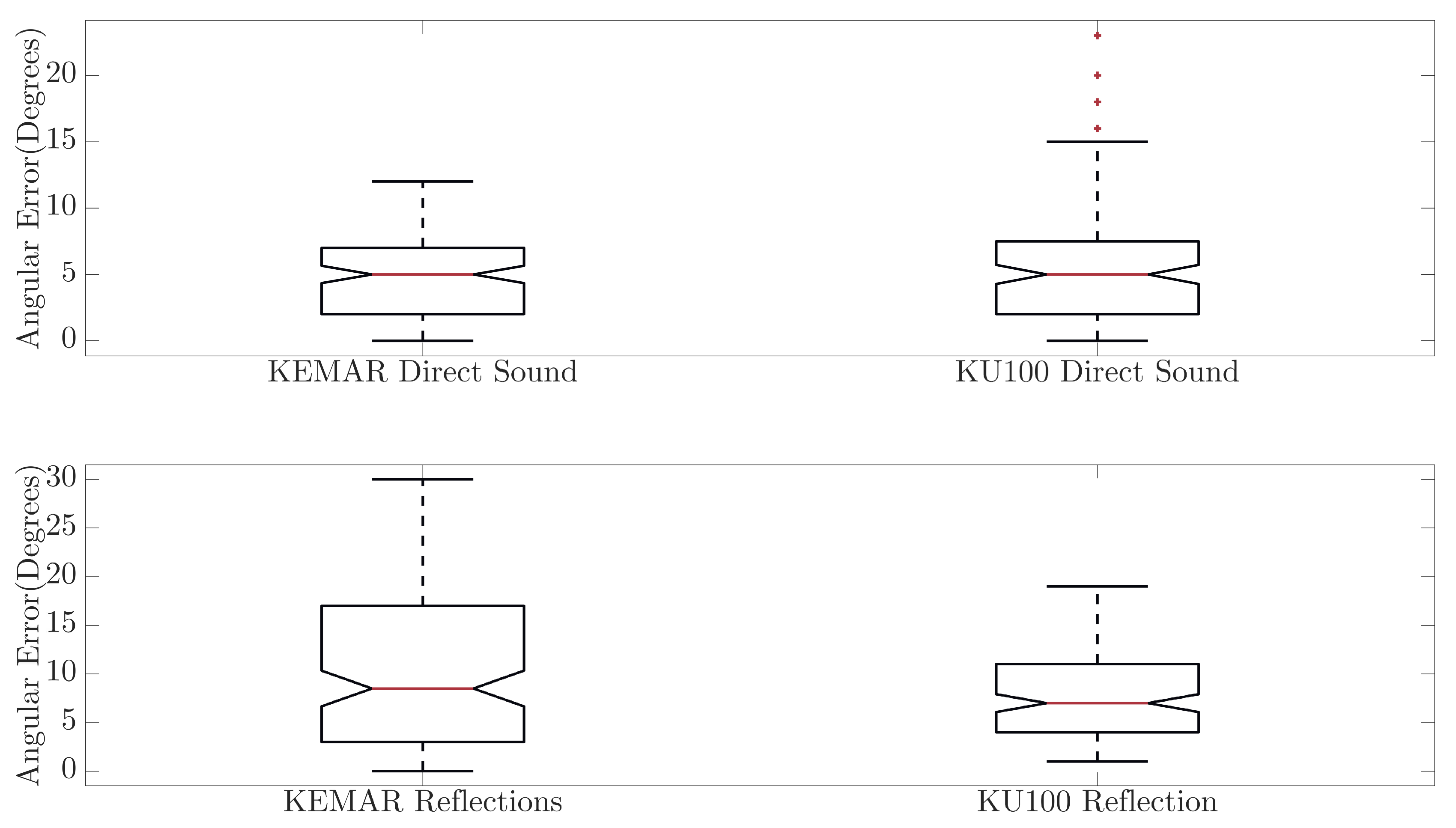
Figure 9.
Comparison of interaural cross correlation across the direction of arrival for the KEMAR measured direct sound (top left), KEMAR measured reflection (bottom left), KU100 measured direct sound (top right) and KU100 measured reflection (bottom right).
Figure 9.
Comparison of interaural cross correlation across the direction of arrival for the KEMAR measured direct sound (top left), KEMAR measured reflection (bottom left), KU100 measured direct sound (top right) and KU100 measured reflection (bottom right).
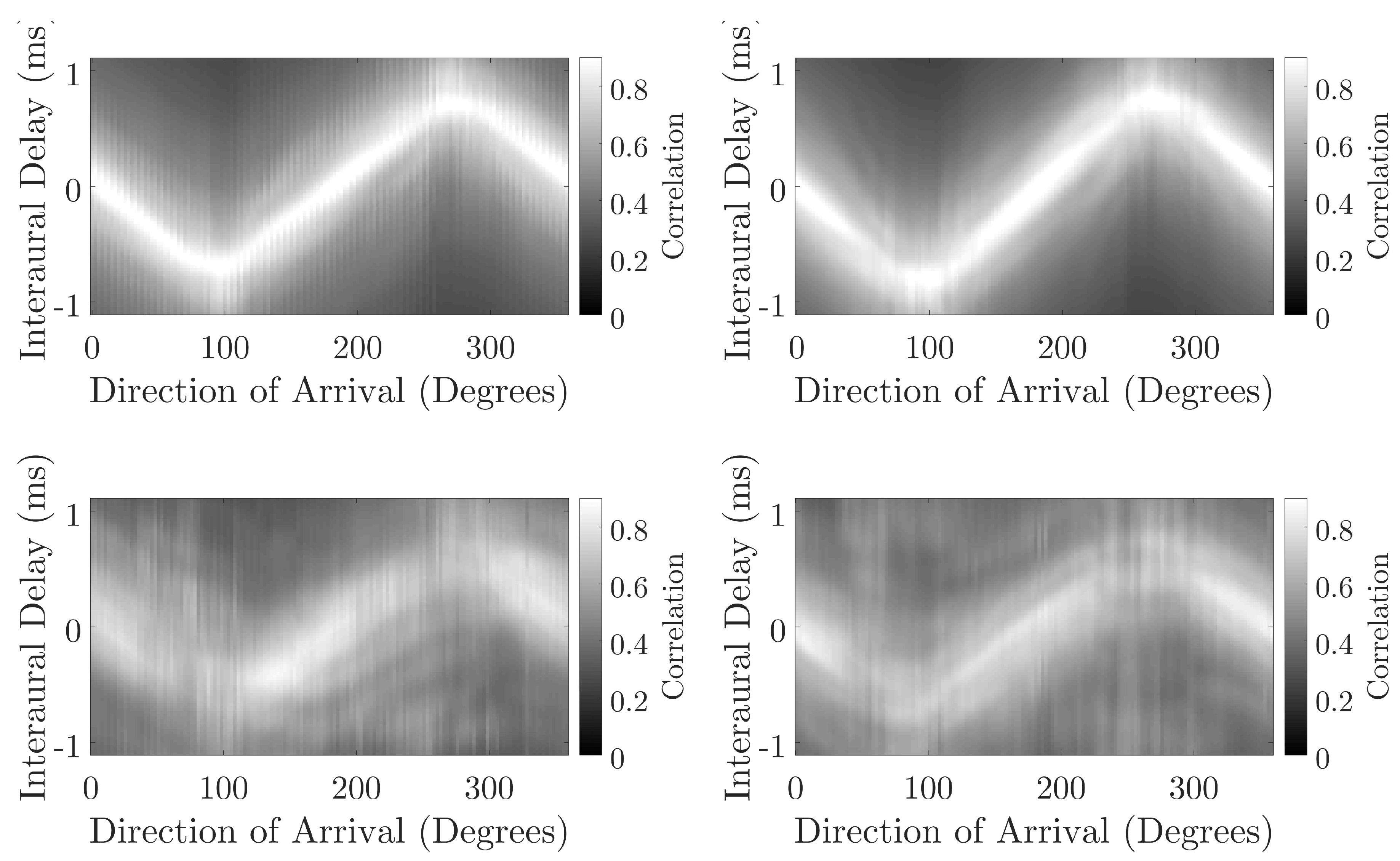
Figure 10.
Comparison of interaural level difference across the direction of arrival for the KEMAR measured direct sound (top left), KEMAR measured reflection (bottom left), KU100 measured direct sound (top right) and KU100 measured reflection (bottom right).
Figure 10.
Comparison of interaural level difference across the direction of arrival for the KEMAR measured direct sound (top left), KEMAR measured reflection (bottom left), KU100 measured direct sound (top right) and KU100 measured reflection (bottom right).
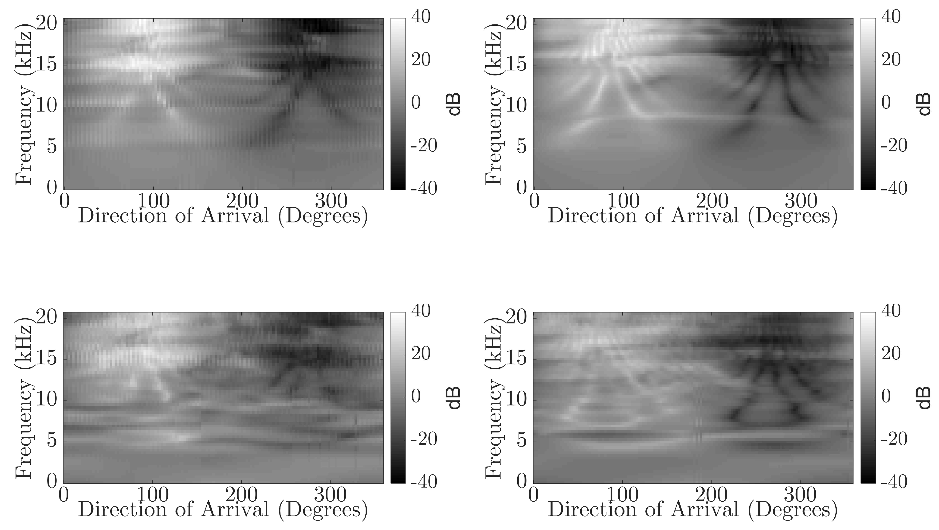
Figure 11.
Plots of neural network predicted direction of arrival (dotted black line) vs. expected direction of arrival (solid line). The top left plot is for the KEMAR direct sound; the top right plot is for the KU100 direct sound; the bottom left is for the KEMAR reflection; and the bottom right is for the KU100 reflections.

Table 1.
Direction of arrival accuracy comparison for the reflected component measured with the KEMAR 45BC for different fixed receiver rotation angles.
Table 1.
Direction of arrival accuracy comparison for the reflected component measured with the KEMAR 45BC for different fixed receiver rotation angles.
| Rotation | Within ±5° | Front-Back Confusions | Max Error |
|---|---|---|---|
| KEMAR Reflections | |||
| ° | 29.86% | 15.28% | 173 |
| ° | 34.03% | 6.25% | 54 |
| ° | 29.17% | 9.72% | 50 |
| ° | 32.64% | 9.03% | 30 |
Table 2.
Comparison of prediction accuracy for the reflected component measured with the KEMAR 45BC using additional measurements at receiver rotations of ° using a multi-layer perceptron and cascade-correlation neural network. Both the multi-layer perceptron and the cascade-correlation neural network had one hidden layer with 128 neurons and an output layer with 360 neurons and were trained using the procedure discussed in Section 2.3.
| Neural Network | Within ±5° | Run Time |
|---|---|---|
| KEMAR Reflections (Test Data) | ||
| multi-layer perceptron | 26.39% | 390 Epochs 40 s |
| cascade-correlation | 32.64% | 244 Epochs 28 s |
Table 3.
Direction of arrival accuracy comparison for the direct sound and reflected components measured with the KEMAR and KU100 binaural dummy heads, for both the cascade-correlation neural network and the baseline method.
Table 3.
Direction of arrival accuracy comparison for the direct sound and reflected components measured with the KEMAR and KU100 binaural dummy heads, for both the cascade-correlation neural network and the baseline method.
| Head | Exact | Within ±1° | Within ±5° | Front-Back Confusions | Average Relative Error | Root Mean Squared Error |
|---|---|---|---|---|---|---|
| Cascade-Correlation Neural Network | ||||||
| Direct Component | ||||||
| KEMAR | 17.36% | 21.53% | 64.58% | 1.39% | 7.10% | 5.18° |
| KU100 | 13.19% | 17.36% | 68.06% | 0% | 6.90% | 6.86° |
| Reflected Component | ||||||
| KEMAR | 2.08% | 11.11% | 32.64% | 9.03% | 23.61% | 13.59° |
| KU100 | 0% | 9.03% | 37.50% | 2.78% | 15.43% | 8.85° |
| Baseline Method | ||||||
| Direct Component | ||||||
| KEMAR | 1.39% | 2.78% | 11.81% | 49.31% | 38.78% | 66.37° |
| KU100 | 1.39% | 3.47% | 13.19% | 50% | 36.01% | 65.66° |
| Reflected Component | ||||||
| KEMAR | 0% | 2.78% | 11.11% | 49.31% | 38.85% | 67.31° |
| KU100 | 0% | 4.86% | 21.53% | 49.31% | 36.81% | 70.23° |
© 2018 by the authors. Licensee MDPI, Basel, Switzerland. This article is an open access article distributed under the terms and conditions of the Creative Commons Attribution (CC BY) license (http://creativecommons.org/licenses/by/4.0/).
Share and Cite
MDPI and ACS Style
Lovedee-Turner, M.; Murphy, D. Application of Machine Learning for the Spatial Analysis of Binaural Room Impulse Responses. Appl. Sci. 2018, 8, 105. https://doi.org/10.3390/app8010105
AMA Style
Lovedee-Turner M, Murphy D. Application of Machine Learning for the Spatial Analysis of Binaural Room Impulse Responses. Applied Sciences. 2018; 8(1):105. https://doi.org/10.3390/app8010105
Chicago/Turabian StyleLovedee-Turner, Michael, and Damian Murphy. 2018. "Application of Machine Learning for the Spatial Analysis of Binaural Room Impulse Responses" Applied Sciences 8, no. 1: 105. https://doi.org/10.3390/app8010105
Note that from the first issue of 2016, this journal uses article numbers instead of page numbers. See further details here.