Electromechanical Anisotropy at the Ferroelectric to Relaxor Transition of (Bi_0.5Na_0.5)_0.94Ba_0.06TiO₃ Ceramics from the Thermal Evolution of Resonance Curves

Abstract

(Bi_0.5Na_0.5)_0.94Ba_0.06TiO₃ dense ceramics were obtained from autocombustion sol-gel synthesized nanopowders and sintered at 1050 °C for 1–2 h for the study of the electromechanical anisotropy. Measurement of the complex impedance spectrum was carried out on thin ceramic disks, thickness-poled, as a function of the temperature from 16 °C up to the vanishing of the electromechanical resonances at the ferroelectric to relaxor transition near 100 °C. The spectrum comprises the fundamental radial extensional mode and three overtones of this, together with the fundamental thickness extensional mode, coupled with other complex modes. Thermal evolution of the spectrum shows anisotropic behavior. Piezoelectric, elastic, and dielectric material coefficients, including all losses, were determined from iterative analysis of the complex impedance curves at the planar, thickness, and shear virtually monomodal resonances of disks and shear plates, thickness-poled. d₃₃ was measured quasi-statically at 100 Hz. This set of data was used as the initial condition for the optimization of the numerical calculation by finite elements of the full spectrum of the disk, from 100 kHz to 1.9 MHz, to determine the thermal evolution of the material coefficients. An appropriate measurement strategy to study electromechanical anisotropy of piezoelectric ceramics has been developed.

1. Introduction

Lead-free ceramics with composition at the solid solution system of (1 − x)(Bi_0.5Na_0.5)TiO₃-xBaTiO₃ (BNBT100x) with x = 0.06 have been widely studied in recent years due to their complex crystal structure, exhibiting a field induced phase transition at the nano-scale between short-range ordered and ferroelectric, long-range ordered, polar states [1,2]. The thermal depolarization accompanied by the inhibition of the piezoelectric activity [1] has a multiple origin [3,4]. On the one hand, there is a thermal randomization of the polarization at the ferroelectric domains. On the other hand, there is a thermally stimulated and non-abrupt transition, without macroscopic symmetry breaking, from the long-range ordered ferroelectric structure induced by the field to an ergodic relaxor at ~100 °C, well below the transition to the non-polar paraelectric phase.

Piezoelectric ceramics in the linear range are modeled using constitutive equations that link two mechanical macroscopic magnitudes, strain S and stress T, with two electric magnitudes, the electric field E and the electric displacement D. The parameters in the constitutive equations give information about macroscopic behavior, however they are related with the microscopic mechanisms. For this reason, we aim to determine all parameters in the constitutive equations as a function of the temperature in order to obtain information about the depolarization process. We use measurements of the complex impedance as a function of the frequency of resonators of a given geometry for this purpose. The analysis of these resonance spectra will be made here using alternative methods to that of current standards for measurements of piezoelectric ceramics [5], at present under revision.

The simplest magnitude to measure the behavior of a piezoelectric ceramics is the electric impedance Z. The electric impedance is a complex number function of the angular frequency ω, if the system remains linear, Z(ω) determines the electric current when a sinusoidal voltage is applied. Almost all piezoelectric ceramic characterization work uses electric impedance or its inverse function, the admittance Y(ω). Sometimes, it is necessary to identify a resonant peak, in this case the electric conductance G(ω) presents a maximum when the electric power consumed by the sample is maximum, G(ω) is the real part of the admittance. For the anti-resonance frequency, the real part of the impedance R(ω) can be used [6].

In the present case, we need a methodology to determine all parameters as a function of the temperature using only one sample. This sample is thermally depolarized, producing changes in the resonance spectrum as a function of temperature. One alternative to do that is using an iterative methodology based in finite-element method (FEM) simulation [6,7,8]. The use of FEM based minimization techniques to obtain the parameters in the piezoelectric models was successfully implemented by several groups in recent years [9,10,11]. This sort of analysis of impedance curves is not yet incorporated in the standard for measurements [5].

FEM simulation gives an impedance curve numerically computed from a certain set of parameters. The methodology makes an optimization to minimize the difference between the numerical and the experimental impedance curves. The simulations are made using axisymmetric elements allowing the complete simulation of a disk using the symmetry. The output is the electrical impedance as a function of frequency, giving all resonances in the disk including radial thickness and coupled modes. This methodology can be applied for ferro-piezoelectric ceramics with axial 6 mm macroscopic symmetry.

Specific problems and material characteristics require the study of a suitable measurement strategy for the determination of a valid full set of material parameters. In this case, we have no additional information about the range of validity of the parameters. For this reason, the FEM optimization is supported by the information obtained from other samples using monomodal resonances.

The techniques based on the iterative analysis of impedance curves consider one-dimensional models and monomodal resonances which use different resonance modes and resonator shapes to identify different material parameters, and also provide an alternative to standard procedures and their results that are appropriated for the three-dimensional modeling of piezoceramics [12,13].

In a previous work, material coefficients of BNBT ceramics were determined as a function of the temperature using an iterative process of analysis of impedance curves at the monomodal electromechanical resonances of thickness-poled thin disks (radial) and plates (shear) [1,4,14]. Measurements were made as the sample was heated. The studied ceramics were obtained by hot pressing (at 800 °C for 2 h) from autocombustion sol-gel powder and recrystallization (at 1050 °C for 2 h) to minimize grain size and non-stoichiometry [15]. Depolarization temperatures were obtained well above 100 °C when they were measured from uncoupled shear resonances of, thickness-poled, thin plates. Shear resonances were still detected at 140 °C [1]. When depolarization was determined from the planar or thickness mode of thin disks, thickness-poled, depolarization took place at 100 °C. This distinct thermal evolution have been observed in the BNBT100x system, not only for BNBT6 [1,4,14], but also for BNBT4 [16,17]. Since each resonance mode studied is related with a different set of material parameters, the observed phenomenology [1,4,14,16,17] reveals the anisotropy of the depolarization process when studied by measurement of the electromechanical resonances. However, in these previous works the resonance modes were measured using different samples, specially constructed to uncouple different resonances.

Here we are exploring the thermal depolarization and related phase transition from measurements in a sample where all modes, both pure and coupled modes, contribute together. In this way, we can assess such electromechanical anisotropy of the thermal depolarization beyond any doubt.

In this work, two different results are presented. On the one hand, the evolution of the resonance modes (radial, thickness, and other complex modes) of a BNBT6 thin disk is evaluated as a function of the temperature. The evaluation is made on the resonance frequency and in the modulus of the electrical impedance. On the other hand, we jointly characterize the thermal evolution of the material parameters, extracted from analysis of the impedance spectra using only one sample by methods that are a feasible and advantageous alternatives to the current standards of measurements.

2. Materials and Methods

Ceramics were prepared from autocombustion sol-gel nanopowders synthesized at 500 °C, from acetate and nitrates, as explained elsewhere [18]. Pressed pellets were sintered in two steps using moderate maximum temperatures (1050 °C for 1–2 h) to avoid loss of volatiles. Thin sintered ceramic disks and plates were electroded at the major faces with silver paste, sintered at 400 °C, and poled in silicon oil bath from 120 °C to 50 °C, cooling with an applied field of 30 KV·cm⁻¹, for 30 min. Shear plates were re-electroded for the electrical measurements.

Measurements of complex impedance of disks and plates were made using precision impedance analyzers (Hewlett-Packard, Palo Alto, CA, USA). Model HP4194A was used for the measurements as a function of the temperature, until the inhibition of the piezoelectricity, in situ at an ad hoc sample-holder with a heating module. The sample holder and the temperature control were specially designed for this application. The 16 °C corresponds to room temperature, after that a 5 °C step was used starting from 35 °C up to 105 °C, since in the first interval (16–35 °C) the variation is irrelevant to the aim of the work.

Model HP4192A-LF, connected to a computer with the appropriate software implemented [19], was used for the in situ iterative analysis of resonance curves.

To obtain the complete parameters set, a minimization of the difference between the numerical and the experimental impedance curve is performed. The literature does not provide a complete matrix characterization of these ceramics that could be used as initial conditions for the numerical calculation of the impedance spectra of a thin disk. In order to determine such an initial condition, comprising 10 material coefficients including all losses—piezoelectric, dielectric, and elastic—the iterative analysis of complex impedance curves [12,13,19] of thin disks and shear plates, thickness-poled, was used. To determine d₃₃, a quasi-static measurement was carried out on a thin disk at 100 Hz using a Berlincourt piezometer (Channel products Inc., Chesterland, OH, USA).

After this first condition, the optimization methodology presented in [6,7] was used. Although there may be more efficient solutions, the methodology based in the Nelder–Mead algorithm [20] is generally robust and easy to implement, which are reasons why it was selected here. This methodology can determine all the complex coefficients in the linear piezoelectric model using only one sample. FEM simulations are performed using square with four nodes using complex numbers for all parameters in the model. The geometry is assumed axisymmetric and the material is assumed homogenous and isotropic. After performing a convergence analysis, the element size is fixed in 10 μm, giving 40 elements for one wave length in the thickness mode frequency. Additional details about the implementation of the methodology and the FEM code are in the work of Perez et al. [6,21].This is suitable for this case when we are looking for the simultaneous evolution of the parameters as a function of the temperature including the coupled modes. There are different ways to express the constitutive equations, here we use the method adopted by the IEEE standard [5].

$$T_p=c_{pq}^E{S}_q-e_{kp}{E}_k$$

(1)

$$D_i=e_{iq}{S}_q+{\epsilon }_{ik}^S{E}_k$$

(2)

Due to symmetry, only 10 independent parameters are used to represent a piezoelectric material with axial 6mm macroscopic symmetry. All parameters are complex numbers in order to take in to account the energy losses. The determination involves five elastic constants ($c_{11}^E$, $c_{12}^E$, $c_{13}^E$, $c_{44}^E$, $c_{33}^E$), three piezoelectric (e₃₁, e₃₃, e₁₅), and two dielectric (${\epsilon }_{11}^S$, ${\epsilon }_{33}^S$). Using the initial seed obtained from the one-dimensional analysis, a sensitivity analysis is performed over the real part of the model. Here we obtain different information for the analysis that follows next. First, most of the sensitivity parameters are optimized first as presented by Perez et al. [5]. Second, the parameters are linked with the different resonance modes in order to found a relationship between the changes in the resonance frequency and the parameter value. Finally, we identify the less sensitive parameters to evaluate the results, for this less sensitive set the results must be compared with other samples using different geometry.

The sensitivity is evaluated using the conductivity G and the resistance R, the results are shown in the next section and in the supplementary materials. Here the classical local sensitivity analysis is used as proposed by Perez et al. [6,7,21]. A global sensitivity analysis [22] is not necessary for the actual purposes.

Finally, the parameters are optimized using the Nelder–Mead algorithm [20]. The simulations are performed using an in-house FEM software in MATLAB that allows the modeling of piezoelectric structures with complex properties. The used element is the four-noded axisymmetric isoparametric piezoelectric 2D solid element. In this case, the grid is squared with 100 μm sides. All simulations in the optimization process use axisymmetric elements. In the next section, the fitting of the simulated impedance and the resonance modes is shown. In order to see the vibration shape for each mode, a 2D simulation is performed using commercial software and presented in the supplementary materials.

3. Results

3.1. Impedance Measurements as a Function of the Temperature

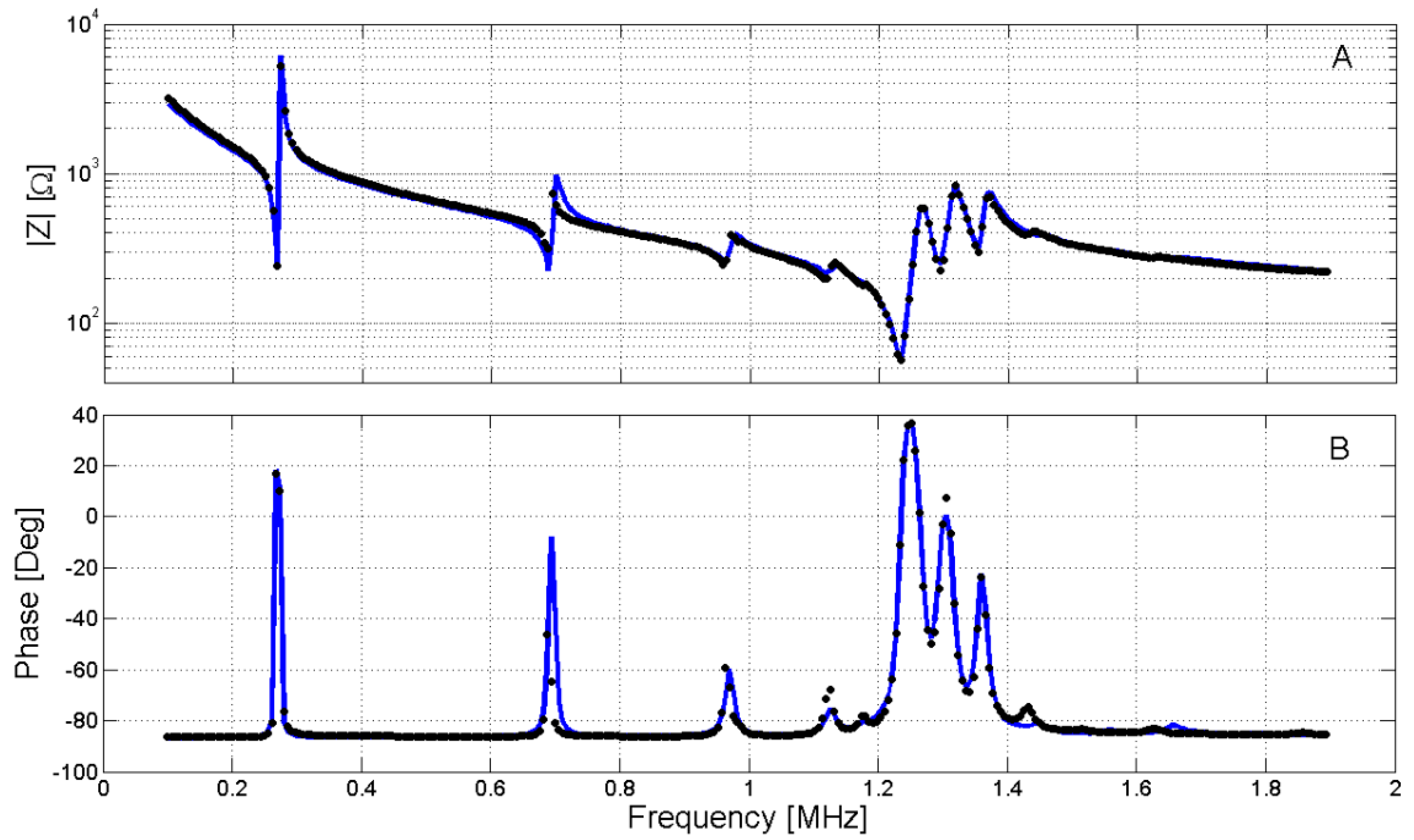
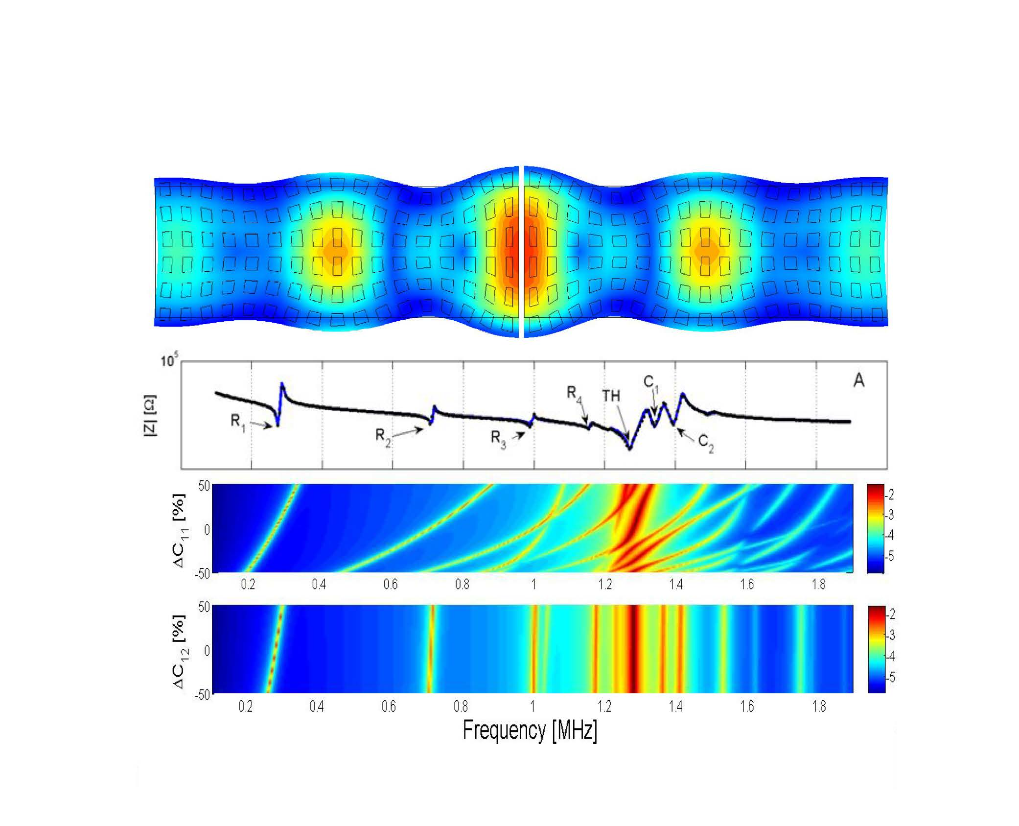
Figure 1A,B shows the measured complex modulus and phase, respectively, measured in the interval from 100 kHz to 1.9 MHz for a BNBT6 thin disk (m = 0.950 g, t = 1.91 mm and D = 10.60 mm) at 35 °C. Figure 1C,D show also an alternative representation of the complex impedance (Z) as the peaks of the real part (Resistance (R)) of Z and the real part (Conductance (G)) of the complex admittance (Y). These peaks are used for the determination of the frequencies of interest for the iterative analysis.

As the fundamental radial resonance is sharp and since the number of points to measure in the spectrum was determined so as to make the problem manageable, the accuracy of determination of |Z|_max for this mode was not sufficient to clearly show the tendency of its thermal evolution. It is here analyzed by the evolution of the overtones (R₂, R₃, R₄).

The spectrum comprises the fundamental radial extensional mode and three overtones of this, together with the fundamental thickness extensional mode and other complex modes [6].

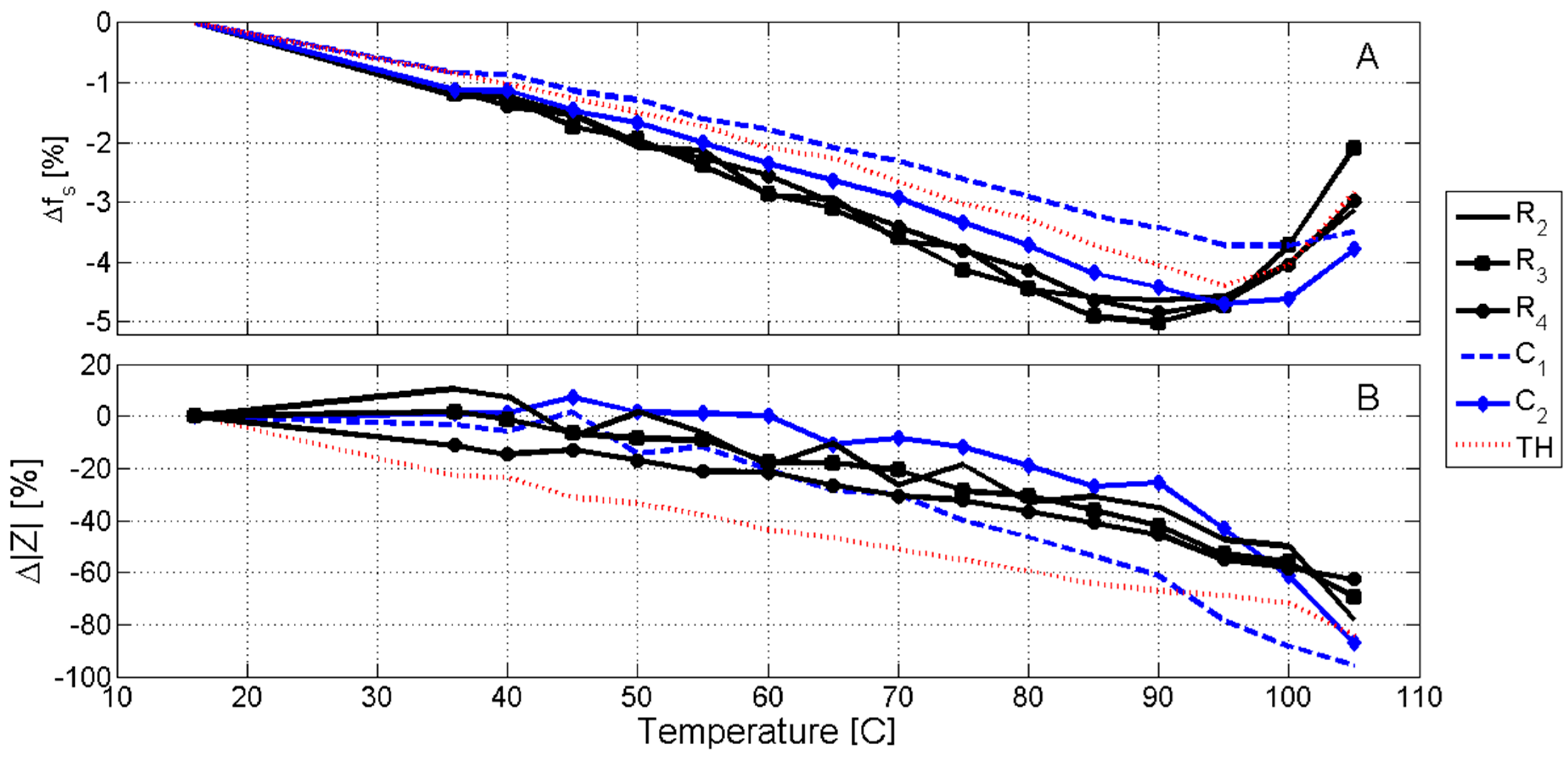
Figure 2A,B shows the evolution of the frequency of resonance and the modulus of the electric impedance for all temperatures. The resonances highlighted in Figure 2 can be observed for all temperatures in the selected range.

From the analysis of Figure 2, we can note a different behavior in the frequencies for the radial modes compared with the thickness and the complex modes. Qualitatively, the frequencies of all modes decrease linearly up to a temperature close to 85 °C. Above this temperature, the frequency increases rapidly. To estimate the temperature of the minimum frequency, a quadratic interpolation is performed near the minimum of each response.

Table 1. Temperature of the minimum in the evolution of the resonance frequency.

Mode	R2	R3	R4	TH	C1	C2
Temperature (°C)	88.5	90.0	90.2	95.0	96.3	97.6

Data interpolated from Figure 2.

shows the results of this interpolation.

As for the impedance modulus, the one for the radial modes decreases monotonically until 85 °C and at a faster rate above this temperature. The inflection point for this decrease is at 100 °C for TH mode and at 90 °C for C₂ mode. However, such an inflection point is not found for C₁ in the measured interval.

Therefore, we found three different tendencies for the thermal evolution of resonances of the: (i) Rn (n = 2, 3, 4) modes; (ii) the TH and C₂ modes; and (iii) the C₁ mode, revealing the electromechanical anisotropy of the thermal depolarization process.

3.2. Iterative Analysis of Impedance Curves

Table 2. Parameters from the iterative analysis of the impedance of thin disks and plates, thickness-poled. Elastic constants are in GPa, piezoelectric constants in C/m².

${\mathit{c}}_{11}^{\mathit{E}}$	${\mathit{c}}_{12}^{\mathit{E}}$	${\mathit{c}}_{13}^{\mathit{E}}$	${\mathit{c}}_{33}^{\mathit{E}}$	${\mathit{c}}_{44}^{\mathit{E}}$	e31	e15	e33	${\mathit{\epsilon }}_{11}^{\mathit{S}}$	${\mathit{\epsilon }}_{33}^{\mathit{S}}$
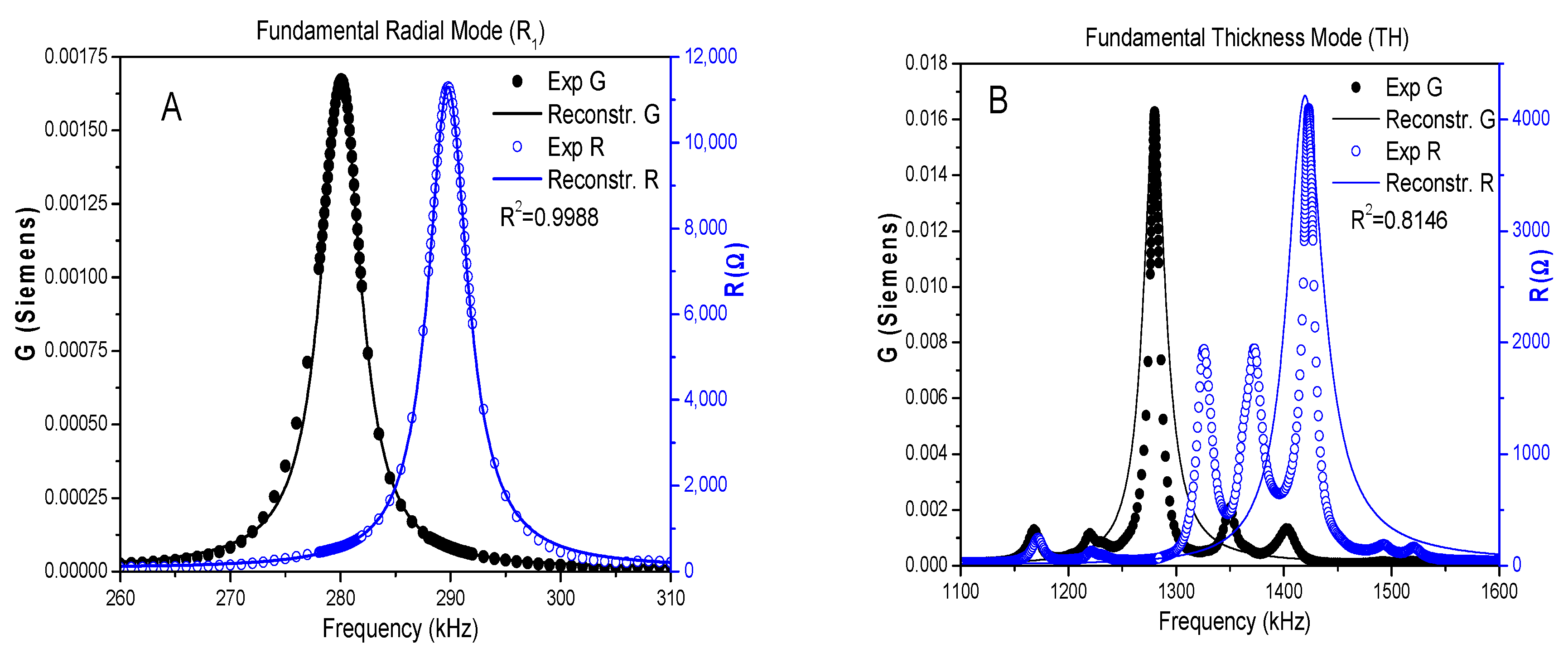
149.9 + j0.42	77.1 + j0.42	74.4 + j0.49	138.1 + j0.45	41.4 + j0.07	−1.47 + j1.23	11.17 + j0.33	6.56 − j0.23	609 − j29	421 − j13

shows the complex material parameters from the iterative analysis of the impedance curves at resonance, that are used as initial condition for the optimization of the numerical calculation of the spectra in Figure 3.

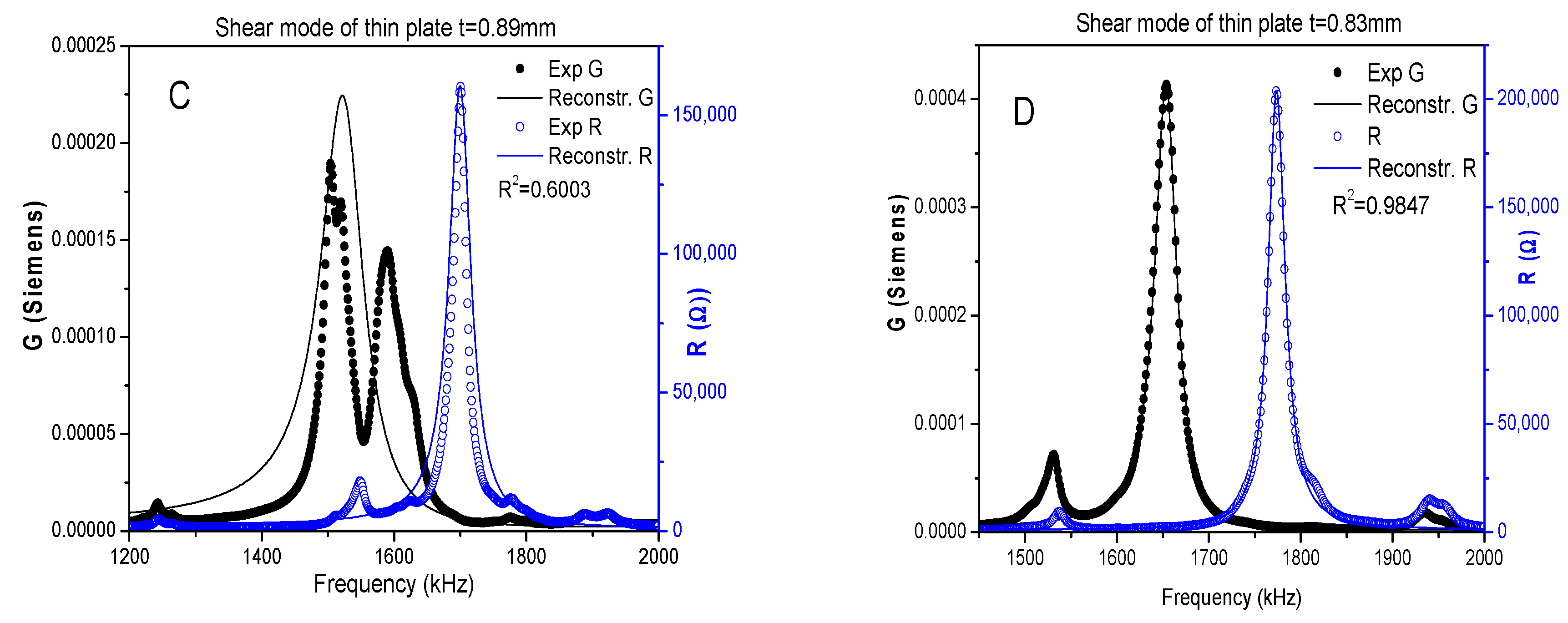
Figure 3A,B show the Resistance (R) and Conductance (G) for the fundamental radial and thickness resonances of the BNBT6 thin disk, thickness-poled (t = 1.91 mm and D = 10.60 mm). These peaks are used for the determination of the frequencies of interest for the iterative analysis. Also, parameters in Table 1 were obtained from the shear mode of a thin plate that initially had 0.89 mm thickness, and lateral dimensions 9.53 and 9.43 mm. This plate was thinned down to 0.83 mm, thus obtaining a decoupled mode. Figure 3C,D show the R and G peaks for the shear mode of the thin plate of 0.83 mm thickness.

3.3. Sensitivity Analysis

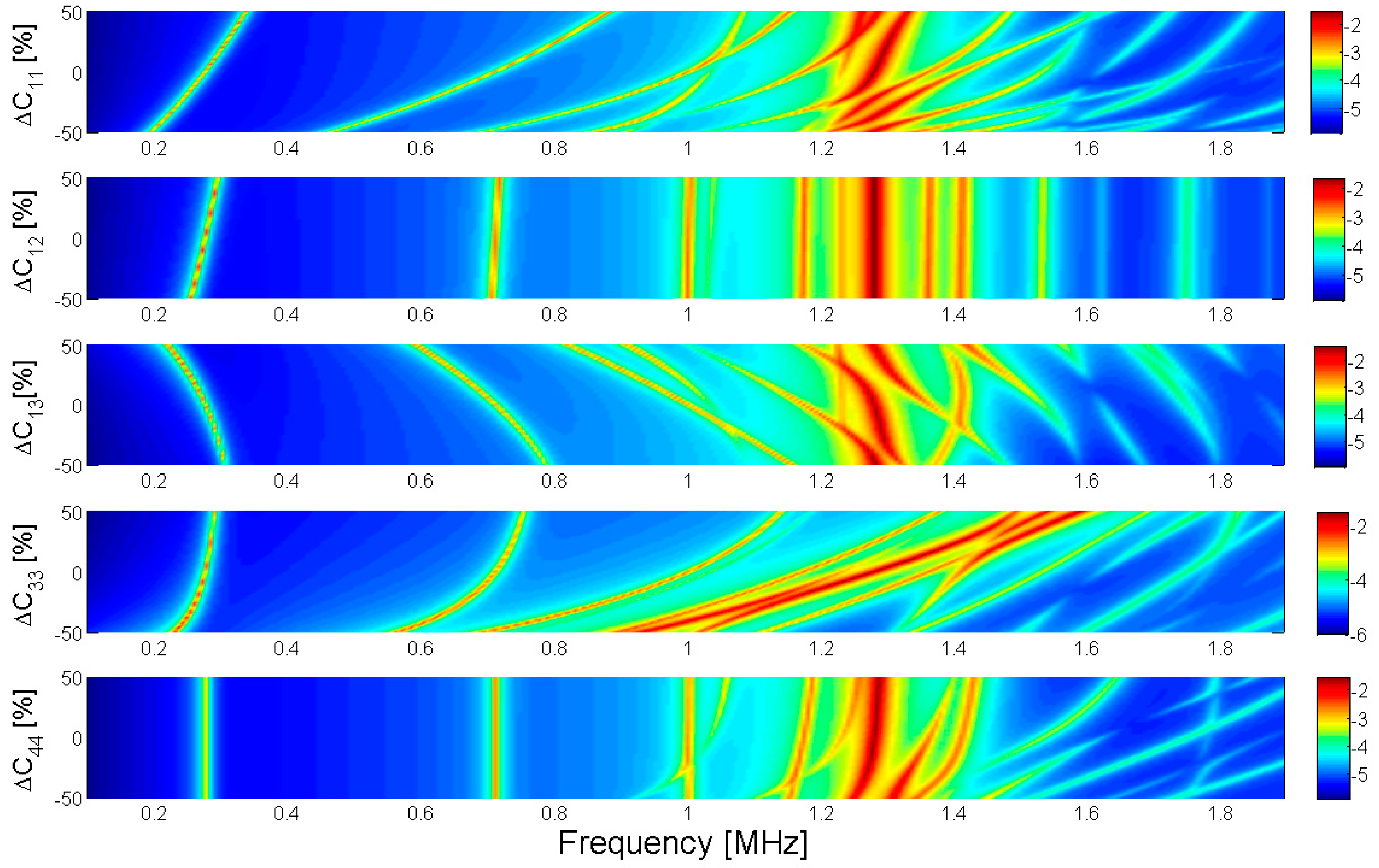
The result of the FEM optimization depends on the right choice of the initial conditions. For this reason, a sensitivity analysis is performed by representing the evolution of the maximum of G and R curves (Figure 1) when each given parameter of the initial condition is changed. The sensitivity analysis is used together with the results of Table 1 to obtain the initial seed in the optimization. Figure 4 shows the sensitivity analysis results for the G curves for each elastic parameter.

This sensitivity analysis for the R curves, together with the analysis for the dielectric and piezoeletric parameters for the G and R curves are given in the Supplementary Materials file (Figures S1–S3).

The sensitivity is computed as the tangent of the angle in the sensitivity maps. According to this, the parameters can be divided into three groups. First, those parameters that provoke clear changes in the spectrum, high sensitivity ones: $c_{11}^E$, $c_{13}^E$, $c_{33}^E$, ${\epsilon }_{33}^S$, and e₃₃. Second, those parameters that provoke some changes in the spectrum, medium sensitivity parameters: $c_{12}^E$, e₁₅, and $c_{44}^E$. Finally, those parameters that practically do not change the spectrum, low sensitivity parameters: e₃₁ and ${\epsilon }_{11}^S$.

We can summarize the sensitivity analysis in

Table 3. Summary of the sensitivity analysis from Figure 4 and similar in the supplementary material.

	c11	c12	c13	c33	c44	e31	e15	e33	ε1	ε33
R1	High	Med.	High	High	Null	Low	Null	Null	Null	Null
R2	High	Low	High	High	Null	Null	Null	Null	Null	Null
R3	High	Low	High	High	Low	Null	Null	Med.	Null	Null
R4	High	Null	High	High	Med.	Null	Low	Med.	Null	Null
TH	Null	Null	Null	High	Null	Null	Null	High	Null	High
C1	High	Null	High	High	High	Null	Med.	Med.	Low	Low
C2	High	Null	High	High	High	Null	Med.	Med.	Low	Low

showing the different influence of each parameter over each of the studied modes. Here we use four steps to characterize the different degrees of sensitivity (null, low, medium, high).

3.4. Optimized Parameters

After the needed changes for the best fit of the initial conditions, a minimization approach for the best fit of the model to the experimental data was carried out.

Table 4. Set of parameters from the optimization for curves at 16, 40, 60, 80, and 100 °C.

T (°C)	${\mathit{c}}_{11}^{\mathit{E}}$	${\mathit{c}}_{12}^{\mathit{E}}$	${\mathit{c}}_{13}^{\mathit{E}}$	${\mathit{c}}_{33}^{\mathit{E}}$	${\mathit{c}}_{44}^{\mathit{E}}$	e31	e15	e33	${\mathit{\epsilon }}_{11}^{\mathit{S}}$	${\mathit{\epsilon }}_{33}^{\mathit{S}}$
16	144.3 + j1.03	52.1 + j0.48	54.7 + j0.56	132.8 + j1.26	39.9 + j0.44	−1.24 + j0.0026	7.72 − j0.005	10.09 − j0.105	1841 − j105	374 − j12
40	141.8 + j1.04	53.2 + j0.48	55.3 + j0.56	130.6 + j1.28	38.3 + j0.43	−1.58 + j0.002	8.85 − j0.006	10.77 − j0.147	1853 − j101	431 − j15
60	139.6 + j1.01	53.0 + j0.47	55.9 + j0.55	128.7 + j1.29	37.0 + j0.44	−1.29 + j0.0019	8.90 − j0.008	11.27 − j0.149	1536 − j141	494 − j19
80	136.7 + j1.04	52.4 + j0.46	55.8 + j0.54	125.1 + j1.32	36.3 + j0.43	−1.83 + j0.0012j	9.46 − j0.009	12.33 − j0.182	1632 − j155	590 − j26
100	134.1 + j1.05	49.9 + j0.47	53.2 + j0.51	125.3 + j1.37	33.9 + j0.42	−1.49 + j0.0013	6.27 − j0.007	12.18 − j0.125	895 − j170	999 − j73

Elastic constants are in GPa, piezoelectric constants in C/m².

shows the set of parameters obtained after minimization of the numerical calculation of the complex impedance spectra of the thin disk as a function of the temperature. The experimental impedance curve was fitted for all temperatures and the parameters are optimized to minimize the quadratic error in the modulus of the electric impedance. The complex part of the model was adjusted, minimizing the error in G and R curves, see Figure 1C,D.

Figure 5 shows the numerical calculation, optimized for 100 °C, here we can observe the differences in shape and magnitude of the spectrum against the data in Figure 1. Although the fitting is poorer than that obtained at room temperature, all resonances are well represented by the numerical model.

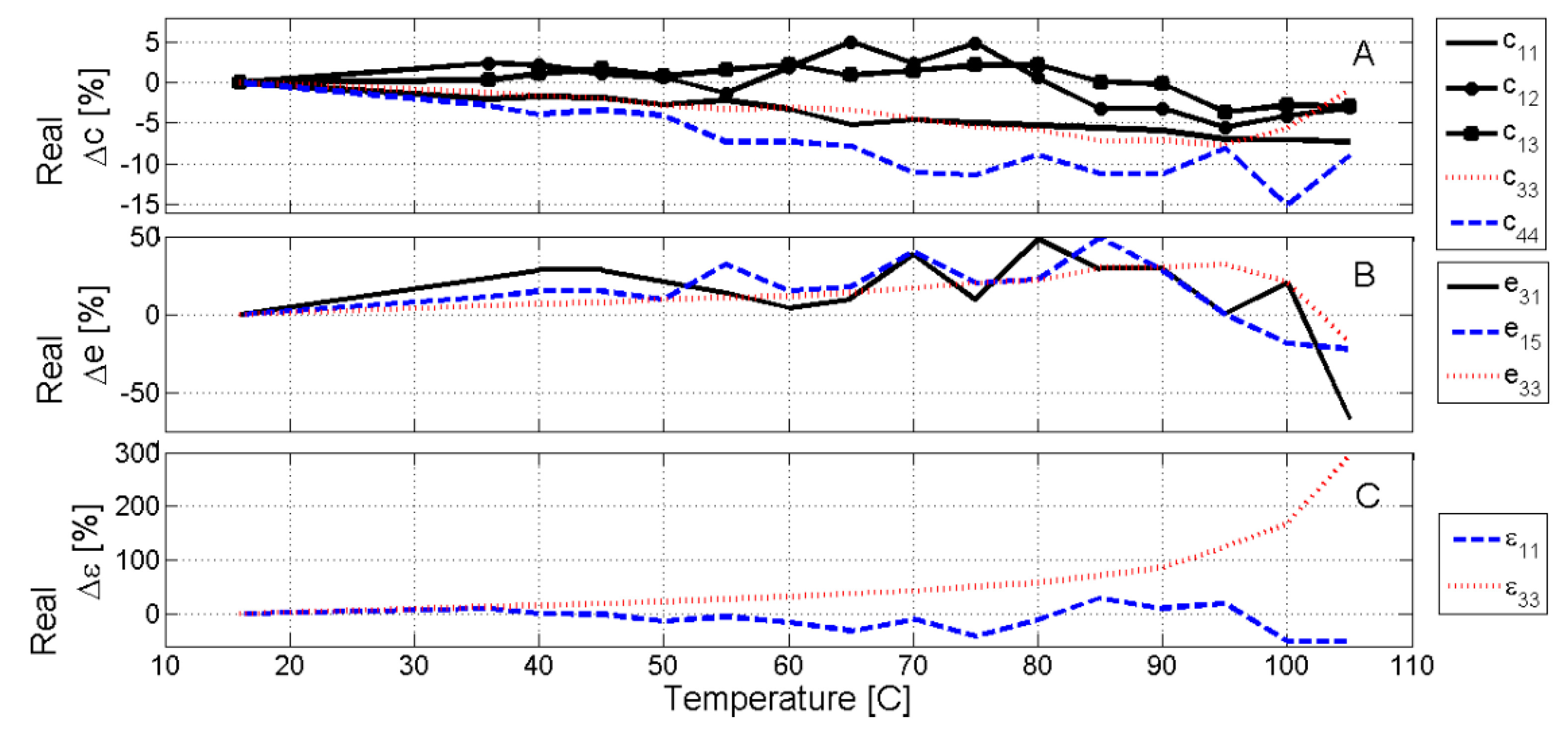
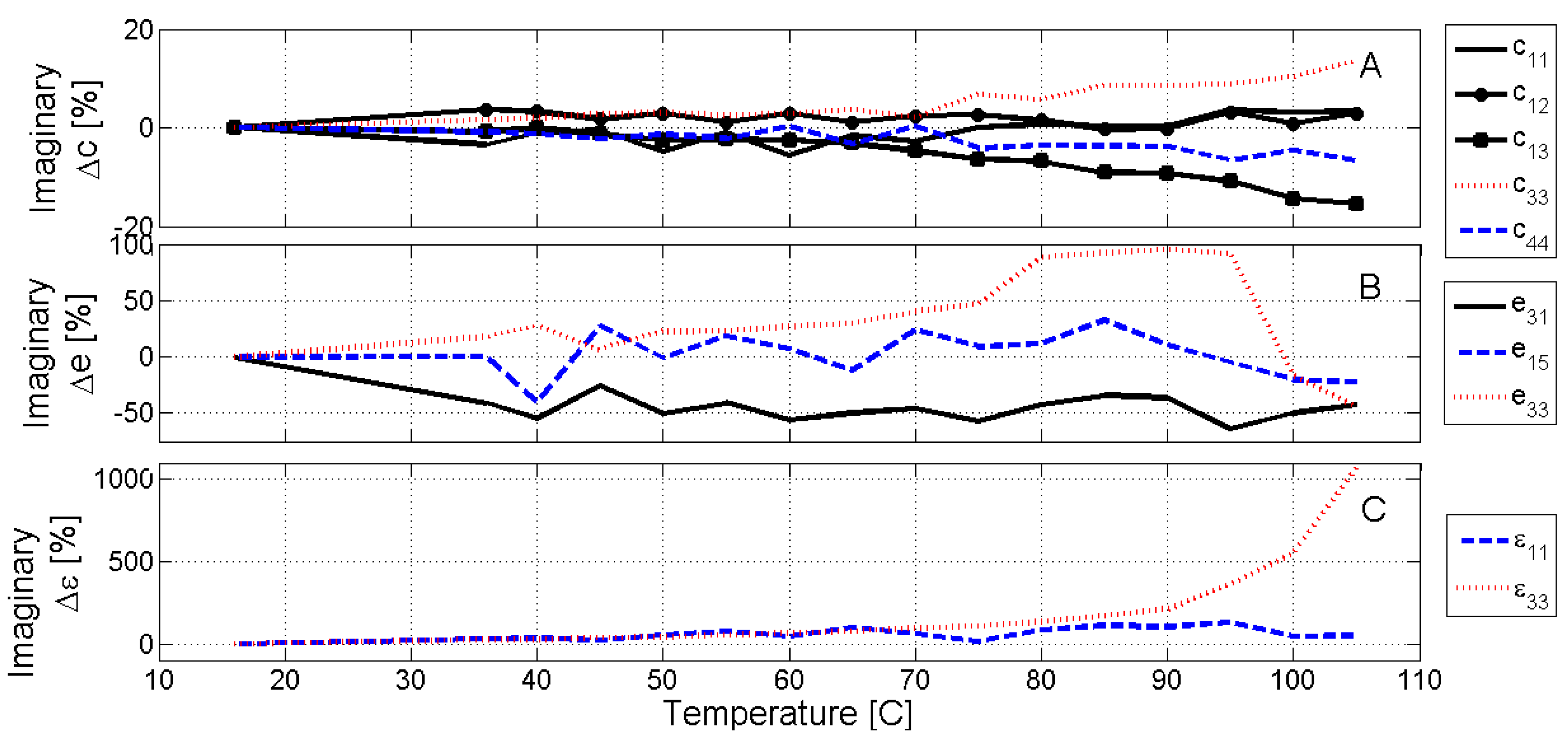
Figure 6 and Figure 7 show the evolution of the real and imaginary part, respectively, of the optimized parameters.

The different scale of thermal changes is noticeable in the depolarization process of the elastic (up to 15% in the real and the imaginary parts), piezoelectric (up to 60% in the real part and 100% in the imaginary), and dielectric parameters (up to 300% in the real part and 1000% in the imaginary).

The dielectric permittivity as a function of the temperature plots show local maxima, dielectric anomalies, revealing the changes in the polar structure of the materials at the phase transitions [1]. The strong anisotropy (Figure 6 and Figure 7) of the dielectric permittivity reveals that the polar changes are related to the polarization parallel to the electric field (three-axis). Thus, the observed changes in the parameters from the optimized numerical calculation of the spectra are compatible with a phase transition with strong change in the polar structure of the material from a ferro-piezoelectric phase to a highly polarizable and non-piezoelectric one.

Both the real and the imaginary parts of all parameters related with the TH mode are high sensitivity ones and their thermal evolution (red lines in Figure 6 and Figure 7) shows smooth changes. The real part of the elastic $c_{33}^E$ follows the evolution of the resonance frequency (Figure 2), having a clear minimum before 100 °C. At the same temperature, the net decrease of both the real and imaginary parts of e₃₃ is observed, as piezoelectric activity vanishes at the ferroelectric to relaxor phase transition [1].

Due to the local maxima at the phase transitions [1], near 100 °C, a faster increase of real and imaginary parts of ${\epsilon }_{33}^S$ is observed as the temperature increases, corresponding to the dielectric anomaly at the ferroelectric to relaxor phase transition. Also, the increase in the mechanical losses (imaginary part of the elastic $c_{33}^E$) is observed.

As for the elastic parameters related with the radial mode of resonance, both the high sensitivity ($c_{11}^E$, $c_{13}^E$) and medium sensitivity ones ($c_{12}^E$), show small but fluctuating changes with the temperature, both in their real and imaginary parts. This is connected with the poorer determination of the characteristic of the sharper resonances. However, even being a low sensitivity parameter, a decrease of the real part of e₁₃ seems to be clear from 80 °C, in agreement with the evolution of both the resonance frequencies and impedance modulus of the radial modes (Figure 2).

Parameter values for 16 °C were used in the FEM modeling of the thin disk to determine the deformation at resonance (see Supplementary Materials Figures S4–S7). This confirms the purely dilatational character of the fundamental radial (R₁) and thickness (TH) modes. It also shows that the deformation at C₁ and C₂ modes involves a great deal of shear movements. With this information, the sensitivity analysis of the Figure 4 and the supplementary material summarized in Table 3, we conclude that the thermal evolution of $c_{44}^E$ and e₁₅, medium sensitivity parameters, and ${\epsilon }_{11}^S$, low sensitivity parameter, should be mostly related with that of the C₁ and C₂ modes. However, those two modes do not change in the same way as the temperature increases (Figure 2). The thermal depolarization weakly affects the real and imaginary part of ${\epsilon }_{11}^S$. The strong fluctuations of $c_{44}^E$ do not mask the continuous decrease as the temperature increases of its real and imaginary parts. However, the fluctuations of e₁₅ make it difficult to make conclusions about the temperature at which the piezoelectric activity linked to it vanishes, though the rate of its decrease near 100 °C is the lowest of the three piezoelectric parameters.

Overall, these differences confirm those revealed by the analysis of the experimental data and are in agreement with the literature on the crystal anisotropy of the BNBT6 ceramics [23].

4. Concluding Remarks

The measurement strategy developed here can determine the complex piezoelectric, dielectric, and elastic parameters, including all losses, as a function of the temperature using only one sample. The initial conditions for the minimization of the differences between the numerically calculated and experimental impedance spectrum were obtained from: (i) the measurement of virtually monomodal resonances in thickness-poled thin disks and plates and (ii) a sensitivity analysis of the parameters. The full impedance spectrum measured for the thin disk comprises the fundamental radial resonance and three overtones, Rn (n = 1, 2, 3, 4), and the fundamental thickness resonance (TH) coupled with other complex modes (Cm (m = 1, 2)).

The electromechanical anisotropy is clearly observed in the experimental data since we found different trends for the thermal evolution of the studied resonance modes.

The thermal evolution of the parameters from the optimized numerical calculation of the experimental spectrum is compatible with a phase transition with strong change in the polar structure of the material from a ferro-piezoelectric phase to a highly polarizable and non-piezoelectric one.

Those parameters that are linked with the radial modes seem to have changes from 80 °C. Near 100 °C, the change of e₁₅ is the lowest of the three piezoelectric parameters, but its fluctuations make it difficult to conclude about the temperature at which the piezoelectricity vanishes. The high sensitivity parameters associated to the thickness mode resonance change critically below 100 °C.