The Study of Non-Detection Zones in Conventional Long-Distance Ultrasonic Guided Wave Inspection on Square Steel Bars

Abstract

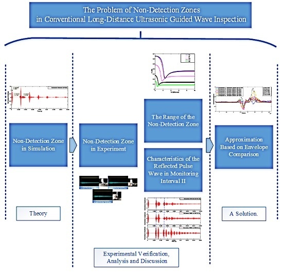
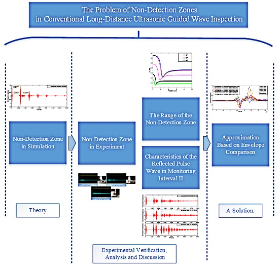
In a low-frequency ultrasonic guided wave dual-probe flaw inspection of a square steel bar with a finite length boundary, the flaw reflected pulse wave cannot be identified using conventional time monitoring when the flaw is located near the reflection terminal; therefore, the conventional ultrasonic echo method is not applicable and results in a non-detection zone. Using analysis and simulations of ultrasonic guided waves for the inspection of a square steel bar, the reasons for the appearance of the non-detection zone and its characteristics were analyzed and the range of the non-detection zone was estimated. Subsequently, by extending the range of the conventional detection time domain, the envelope of the specific reflected pulse signal was extracted by a combination of simulations and related envelope calculations to solve the problem of the non-detection zone in conventional inspection methods. A comparison between the simulation and the experimental results demonstrate that the solution is feasible. This study has certain practical significance for ultrasonic guided wave structural monitoring.

1. Introduction

Currently, ultrasonic guided wave inspection is an effective long-distance nondestructive inspection technique [1,2,3]. Low-frequency ultrasonic guided waves are widely used for long-distance ultrasonic guided wave inspection [4]. The ultrasonic pulse width is wider at low frequency than at high frequency. Due to the influence of the pulse dispersion for long-distance transmissions, the reflected signal pulse is wider than in short-distance transmission [5]. The superposition state occurs easily during actual waveform measurements when the flaw is close to the terminal. In addition, the signal trailing interference aggravates the superposition state and the flaw reflected pulse is more difficult to distinguish. In the low-frequency ultrasonic guided wave flaw inspection experiments for a steel square bar as described in this study, we find that the reflected pulse wave of the flaw ‘disappears’ before the first terminal reflected pulse wave (in the conventional monitoring interval) when the flaw is near the reflection terminal; this results in a loss of the flaw’s location information, which is referred to as the non-detection zone in this paper. Therefore, the conventional ultrasonic echo method is invalid under this condition. The literature does not provide clear details on low-frequency ultrasonic guided wave excitation pulse conditions and no studies have focused on providing a solution for the problem of the non-detection zone mentioned in this study. However, the non-detection zone cannot be ignored in studies on nondestructive testing (NDT). In this study, we designed experiments and simulations for the inspection of a square steel bar with the focus on the above-mentioned problem.

Research on ultrasonic reflected pulse waves should be concerned with solving the problem of the non-detection zone to facilitate the actual detection of flaws. To determine the ultrasonic propagation characteristics caused by different types of flaws or structural damages, the reflected pulse wave is used to analyze the reflection and transmission. In reference [5] the flaws of different opening angles were analyzed and in reference [6], the first reflected pulses in a 20–45 Hz range for four sizes and three orientations of transverse rail head flaws were investigated. Moreover, the reflected pulse wave was used to locate the flaws. For example, the flaws in a steel rail flange were detected in reference [7] and the orientation and position of small flaws in pipes were detected in reference [8]. In previous studies, researchers have provided considerable advances in long-distance non-destructive testing (NDT). However, in most studies, the flaw-reflected pulse before the first terminal reflected pulse wave was used to locate and identify the flaw, a method we refer to a “monitoring Interval I” hereafter. Different from the methods used in existing studies, the analysis time domain of the reflected pulse waves is expanded to the “monitoring Interval II” in the following sections. In order to resolve the non-detection zone problem in long-distance low-frequency ultrasonic guided wave detection, a feasible solution to locate the flaw is proposed in this study.

To describe the non-detection zone clearly, the cause of the existence of the non-detection zone is clarified by using a simulation with an equivalent model of low-frequency ultrasonic guided waves for the inspection of a square steel bar in Section 2.The experimental platform and the results are described in Section 3. The characteristics of the non-detection zone are analyzed and discussed. Based on the characteristics of the reflected pulse waveform in the non-detection zone, a solution is proposed. Finally, the experimental verification is described in Section 4.

2. Theory of the Non-Detection Zone

Based on previous research in low-frequency ultrasonic guided wave detection [9,10], we use a square steel bar as an example and analyze the objective reasons for the appearance of the non-detection zone with a finite-length boundary. Firstly, this problem associated with the ultrasonic guided wave (UGW) becomes equivalent to the reflection of waves with different modes in a plate [11] and is the 2D equivalent of an ultrasonic guided wave simulation model. By taking full advantage of the characteristics of the low-frequency pulse wave [12], an analysis is performed on the changes in the pulse signal of the flaw identification and the creation of the non-detection zone in a conventional inspection.

Prior to the analysis of the ultrasonic guided wave echo experiments and simulations, the following constraints are defined:

• A single low-frequency incident pulse is used in the experiments and simulation and the waveforms of the other frequencies are not induced by the excited incident pulse at the corresponding frequencies.
• The mode of the incident pulse wave is a single S0 mode and the frequency of the incident pulse is lower than the S1 and A1 cut-off frequencies so that the mode is simplified and easy to analyze [13].
• In a symmetrical plate-like structure, the reflected pulse is also a single mode S0; in an asymmetrical plate-like structure (such as man-made flaws), the reflected pulses in the A0 mode and S0 mode are excited [14].
• When the frequency-thickness product ($f\cdot d$) is maintained, the group velocity of the S0 and A0 modes remains unchanged under ideal conditions [15].

2.1. The Equivalent Model of Low-Frequency Ultrasonic Guided Wave in a Square Steel Bar

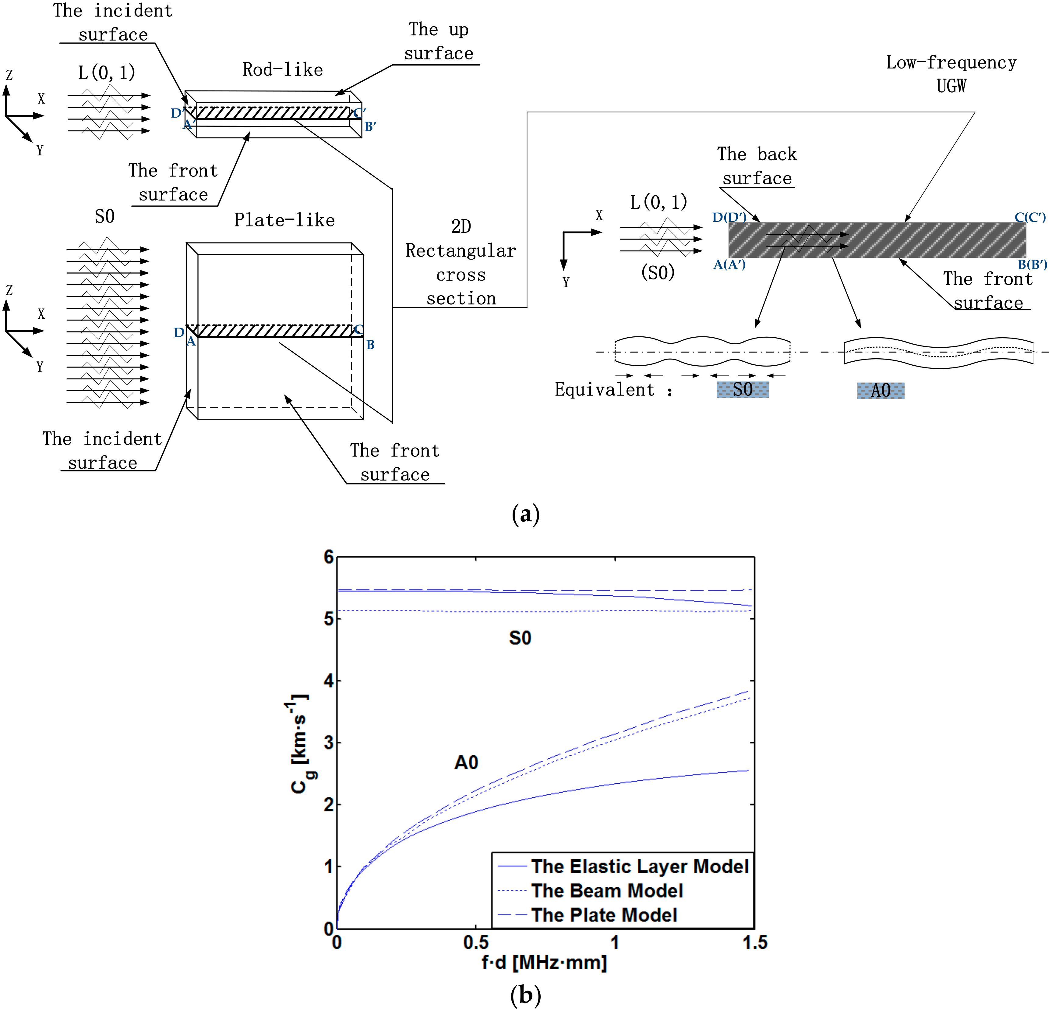
The square steel bar has a symmetric structure and we only focus on the propagation characteristics of the ultrasonic guided wave propagated between the front surface and the back surface, as shown in Figure 1a. We ignore the shear (SH) wave and the other two surfaces (the up surface and the down surface); therefore, this is equivalent to a two-dimensional (2D) model where the ultrasonic Lamb waves propagate along a plate [1,3].

2.1.1. The Mode Selection of Ultrasonic Guided Wave

Based on previous research findings, the reasons for the mode selection of ultrasonic guided wave in this study are as follows:

Firstly, the use of low-frequency ultrasound in long-distance ultrasonic guided wave inspection is preferred because the attenuation of the high-frequency ultrasound transmission over long distances is too fast, which limits the measuring distance [4]. High-frequency ultrasound waves tend to be concentrated on the surface or in localized areas of the propagation medium [1]; therefore, the meaning of detecting the ultrasonic guided wave as the body wave in the entire medium is lost. Because of the multi-mode caused by the high-frequency ultrasonic excitation, the identification of detection becomes difficult. In short, the low-frequency section and less-mode ultrasound are appropriate for the detection requirements of long-distance ultrasonic guided wave inspection. For example, a similar low-frequency ultrasonic guided wave equivalent simulation was applied to rails (a rod-like structure) by Bartoli et al. [7].

Secondly, the simulated effect of an ultrasonic equivalent model is better in the low-frequency range than in the high-frequency range. For the long wavelength in the low-frequency ultrasonic range, the equivalent model for a rod-like structure is similar to the model of a plate-like structure for the Lamb wave mode in a uniform medium. However, the mode distribution generated by the high-frequency section in a rod-like structure is not similar to the Lamb wave mode, thus there is no equivalent effect [3].

Finally, the equivalent model of low-frequency ultrasonic guided waves takes full advantage of the proven Lamb theory and can be used to theoretically control the modes of the excited pulse wave and the mode number [16,17]. The relationship between the S0/A0 impulsive waves and the flaw in related research can be used to analyze the mode transformation under the finite boundary conditions used in this study. Therefore, we use the ideal assumptions described in Section 2.

2.1.2. Theory on the Equivalent Model in Low-Frequency

The three-dimensional model of the steel square bar is set in the Cartesian coordinate system (x, y, z), as shown in Figure 1a. The independent of z deformation is specified by the displacement vector $\overrightarrow{u}=(u_1,u_2,0)$ lying in the plane (x, y), where u₁, u₂, u₃ represent the displacement variable in the x, y, z directions respectively, and the model has a similar 2D plane-strain deformation in the plate-structure. The similar theoretical analysis on the equivalent model for low frequency ultrasonic wave has been proposed by Glushkov et al. [18]. We can see the similar low-frequency phase velocities of S0 and A0 modes provided by the beam and plate models for an aluminium sample in the reference [18], as shown in Figure 1b. In low frequency, this conclusion, that the axisymmetric longitudinal mode in the rod with diameter d is very similar to the symmetric mode distribution in the plate with the same thickness d, is proposed by Rose [2]. In this paper, when we focused on vibration mode S0/A0, without regard to other vibration modes, the ultrasonic wave propagation analysis is simplified and equivalent in low frequency.

In essence, the three-dimensional (3D) ultrasonic wave in the rod is equivalent to the two-dimensional (2D) Lamb wave in this study, which is used as the equivalent model of the low-frequency ultrasonic guided waves in a square steel bar. Both ultrasonic guided wave models are based on the same acoustic propagation control equations [1]. When low frequency ultrasonic wave excitation covers the entire incident surface, as shown in Figure 1a, the rectangular cross-section of ABCD in the plate-like structure is used to ‘replace’ the rectangular cross section ‘A’ ‘B’ C ‘D’ in the rod-like structure for the vibration mode analysis, and the vibration of ultrasonic wave between the front and back surfaces in rod-like structure can be equivalent to the vibration of ultrasonic wave between the front and back surfaces in the plate-like structure. A similar ultrasonic guided wave mode is obtained [3], the longitudinal wave L (0, 1) and the flexural wave F (1, 1) are similar to the S0 and A0 waves respectively in a 2D plate-like ultrasonic propagation. The simulations of the pulse waveform and the actual waveform exhibit good consistency. Compared with the 3D model, the estimation accuracy is slightly lower but the equivalent model reduces the simulation hardware requirements and computational costs, thereby improving the simulation efficiency.

In solid matter, as shown in Figure 1a, the vector form of the wave equation for the ultrasonic wave can be represented as follows [1]:

$$(\lambda +\mu )\nabla (\nabla •\overrightarrow{u})+\mu {\nabla }^2\overrightarrow{u}+(\frac{{\lambda }^{\prime }+{\mu }^{\prime }}{\omega })\nabla (\nabla •\frac{\partial \overrightarrow{u}}{\partial t})+(\frac{{\mu }^{\prime }}{\omega }){\nabla }^2\frac{\partial \overrightarrow{u}}{\partial t}=\rho \frac{\partial \overrightarrow{u}}{\partial t}$$

(1)

where $\lambda$ and $\mu$ are the Lame constants; ${\lambda }^{\prime }$ and ${\mu }^{\prime }$ denote the attenuation factor in the medium.

$${\nabla }^2=\frac{{\partial }^2}{\partial x_{}^2}+\frac{{\partial }^2}{\partial y_{}^2}+\frac{{\partial }^2}{\partial z_{}^2}$$

(2)

$$\nabla ={\overrightarrow{i}}_1\frac{\partial }{\partial x}+{\overrightarrow{i}}_2\frac{\partial }{\partial y_{}}+{\overrightarrow{i}}_3\frac{\partial }{\partial z}$$

(3)

$$\overrightarrow{u}=(u_1,u_2,u_3)$$

(4)

The vector $\overrightarrow{u}$ is treated with the Helmholtz decomposition; u₁, u₂, u₃ represent the displacement variable in the x, y, z directions respectively; therefore, the displacement can be expressed as follows:

$$\overrightarrow{u}=\nabla \overrightarrow{\mathrm{\Phi }}+\nabla \times \overrightarrow{\mathrm{{\rm H}}}$$

(5)

$$\nabla •\overrightarrow{\mathrm{{\rm H}}}=0$$

(6)

where $\overrightarrow{\mathrm{\Phi }}$ and $\overrightarrow{\mathrm{{\rm H}}}$ are the scalar and vector potentials, respectively.

Two simple wave equations can be derived as follows:

$$(\lambda +2\mu +\frac{{\lambda }^{\prime }+2{\mu }^{\prime }}{\omega }\frac{\partial }{\partial t}){\nabla }^2\overrightarrow{\mathrm{\Phi }}=\rho \frac{{\partial }^2\overrightarrow{\mathrm{\Phi }}}{\partial t^2}$$

(7)

$$(\lambda +\frac{{\mu }^{\prime }}{\omega }){\nabla }^2\overrightarrow{\mathrm{{\rm H}}}=\rho \frac{{\partial }^2\overrightarrow{\mathrm{{\rm H}}}}{\partial t^2}$$

(8)

where $\omega$ denotes the angular frequency. If the solutions of Equations (7) and (8) are assumed to be planar harmonic waves, then

$$\overrightarrow{\mathrm{\Phi }}(\overrightarrow{x},t)=\overrightarrow{\mathrm{\Phi }}(\omega )e^{j\omega (\overrightarrow{N}•\overrightarrow{x}/\alpha -t)}$$

(9)

$$\overrightarrow{\mathrm{H}}(\overrightarrow{x},t)=\overrightarrow{\mathrm{{\rm H}}}(\omega )e^{j\omega (\overrightarrow{N}•\overrightarrow{x}/\beta -t)}$$

(10)

where $\overrightarrow{N}$ represents the displacement vector, for the longitudinal wave, the expression of the material parameter $\alpha$ is as follows:

$$\alpha =\frac{\omega }{{\kappa }_{\mathrm{re}1}+i\left|{\kappa }_{im1}\right|}$$

(11)

where ${\kappa }_{\mathrm{re}1}$, ${\kappa }_{im1}$ represent the real part and the imaginary part of the plural of the longitudinal wave number ${\kappa }_1$ respectively.

For transverse wave, the expression of the material parameter $\beta$ is as follows:

$$\beta =\frac{\omega }{{\kappa }_{\mathrm{re}2}+i\left|{\kappa }_{im2}\right|}$$

(12)

where ${\kappa }_{\mathrm{re}2}$, ${\kappa }_{im2}$ represent the real part and the imaginary part of the plural of the transverse wave number ${\kappa }_2$ respectively.

The stress in the z direction $N_3=0$, consequently Equations (9) and (10) can degenerate into a 2D plane strain problem, then $\frac{\partial }{\partial z}=0$.

For the longitudinal wave, the displacement vector is

$${\overrightarrow{u}}_L=\nabla \overrightarrow{\mathrm{\Phi }}=\{\frac{\partial }{\partial x},\frac{\partial }{\partial y},0\}\overrightarrow{\mathrm{\Phi }}$$

(13)

The substitution of Equation (9) into Equation (13) leads to the following equations:

$$u_{L1}=\frac{\partial \overrightarrow{\mathrm{\Phi }}(\overrightarrow{x},t)}{\partial x_{}}=i\omega \frac{N_1}{\alpha }\overrightarrow{\mathrm{\Phi }}(\omega )e^{i\omega (N_{1}x/\alpha +N_{2}y/\alpha -t)}$$

(14)

$$u_{L2}=\frac{\partial \overrightarrow{\mathrm{\Phi }}(\overrightarrow{x},t)}{\partial y}=i\omega \frac{N_2}{\alpha }\overrightarrow{\mathrm{\Phi }}(\omega )e^{i\omega (N_{1}x/\alpha +N_{2}y/\alpha -t)}$$

(15)

$$u_{L3}=0$$

(16)

where $u_{L1}$, $u_{L2}$, $u_{L3}$ represent compressional component in x, y, z three directions respectively.

From the formula derived in reference [3], when the longitudinal wave propagates, the normal stress ${\sigma }_{22}$ and the shear stress ${\sigma }_{12}$ are expressed as:

$${\sigma }_{22}=(\alpha -2N_1^2{\beta }^2/\alpha )i\omega \beta e^{i\omega (\overrightarrow{N}•\overrightarrow{x}/\alpha -t)}$$

(17)

$${\sigma }_{12}=2i\omega \rho N_1{N}_2{\beta }^2/\alpha e^{i\omega (\overrightarrow{N}•\overrightarrow{x}/\alpha -t)}$$

(18)

where $\rho$ represents the material density, when the transverse wave propagates, the normal stress ${\sigma }_{22}$ and the shear stress ${\sigma }_{12}$ are expressed as:

$${\sigma }_{22}=-2i\omega \rho N_1{N}_2\beta e^{i\omega (\overrightarrow{N}•\stackrel{\rightharpoonup }{x}/\beta -t)}$$

(19)

$${\sigma }_{12}=i\omega (N_2^2-N_1^2)\beta /\alpha e^{i\omega (\overrightarrow{N}•\stackrel{\rightharpoonup }{x}/\beta -t)}$$

(20)

where $c_p$ represents the phase velocity of sound, and $s$ represents the Snell constant. The up going wave $N_1=c_{p}s$, $N_2={(1-c_p{}^2{s}^2)}^{\frac{1}{2}}$, and the down going wave $N_1=c_{p}s$, $N_2=-{(1-c_p{}^2{s}^2)}^{\frac{1}{2}}$, when $c_p=\alpha$, longitudinal wave; when $c_p=\beta$, transverse wave.

2.2. Non-Detection Zone in Simulation

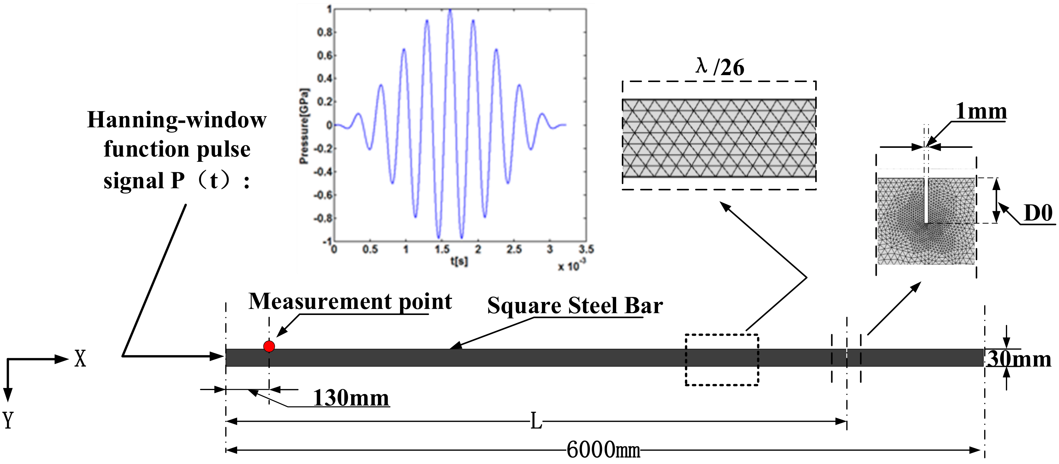
To investigate the reasons for the appearance of the non-detection zone, we focus on the simulations of the propagation of an ultrasonic guided wave in a square steel bar with a length of 6000 mm using COMSOL Multiphysics, ver.5.0.

As shown in Figure 2, during which a 10-pulse Hanning-window function pulse signal with a frequency of 30 kHz is used as the incident pulse.

The Hanning function is used as the window function:

$$Hanning(t)=(1-\cos (2\pi t/T))/2$$

The type of excitation signal:

$$p(t)=\sin (2\pi f_{0}t)Hanning(t)$$

where $T\hspace{0.17em}=\hspace{0.17em}1.6\hspace{0.17em}\left[\mathsf{\mu }\mathrm{s}\right]$.

The point (130, 30) is used as the measurement point and is the same as in the actual experiment in Section 3. A transverse flaw with a depth of 5 mm (D0) and a width of 1 mm is created at the displacement L with a variable value of L $\in$ [3500 mm, 5500 mm] along the x direction from the incident point and the simulation interval is set as 500 mm. (D0 is set as 5 mm for reducing the superposition of the flaw reflected pulses). A triangular grids (λ/26) are used in this study (<λ/20 recommended minimum mesh size [19]) and the area near the location of the flaw L is refined using a local mesh. During the simulation, the excitation energy is properly decreased so that 5 pulses are reflected. The material parameters of the steel square bar are the following:

• Young’s modulus: $E=200\hspace{0.17em}[\mathrm{GPa}]$
• Density: $\rho =7850\hspace{0.17em}[{\mathrm{kg}/\mathrm{m}}^3]$
• Poisson’s ratio: $\nu =0.3$

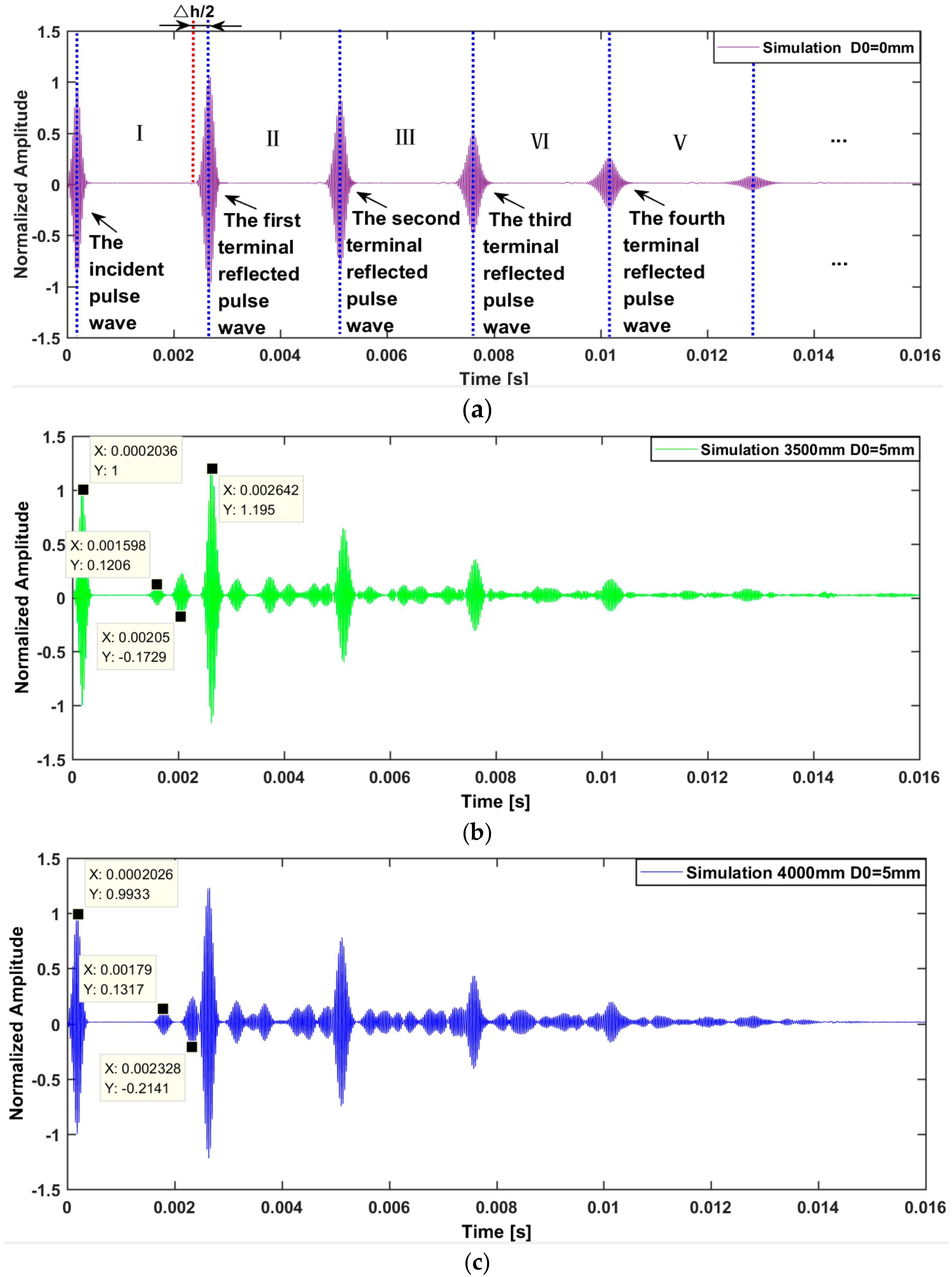
Taking advantage of the periodicity of the terminal reflection, as shown in Figure 3a, the time domain is divided into the monitoring time Interval I, the monitoring time Interval II, the monitoring time Interval III, and so on. The pulse waves of the multiple reflections are labeled as the incident pulse wave, the first terminal reflection pulse wave, the second terminal reflection pulse wave, and so on.

As shown in Figure 2b, at L = 3500 mm, an S0 mode wave is emitted from the incident face and is then reflected by the transverse flaw [20]; then, after the reflection, two different types of waves, S0 and A0, are generated. In Interval I, the peak points of the S0 mode and A0 mode flaw-reflected pulse waves are (0.001598, 0.1206) and (0.00205, −0.1729), respectively. Based on the simulation results, the S0 mode flaw-reflected pulse wave is calculated to verify whether the detected location of the flaw was accurate.

It is known that the first terminal-reflected pulse wave and the initial pulse exhibit the maximum amplitude at ((0.0002036, 1) and (0.002642, 1.195)); the S0 wave group velocity ($C{g}_{S0}$) was calculated as:

$$C{g}_{S0}=\Delta s/\Delta t=(6-0.13)\times 2/(0.002642-0.0002036)=4814.6325\hspace{0.17em}[\mathrm{m}/\mathrm{s}]$$

(21)

where $\Delta s$ and $\Delta t$ represent the propagation distance and the corresponding time respectively. Using the calculated $C{g}_{S0}$, the flaw-induced S0 mode reflected wave is verified. The S0 mode pulse wave appears at 0.001598 s and $L_0$ denotes the distance between the transverse flaw and the initial face, the following expression can be acquired:

$$L_0=(C{g}_{S0}\times \Delta t)/2+0.13=C{g}_{S0}\times (0.001598-0.0002036)/2+0.13=3.4868\hspace{0.17em}[\mathrm{m}]$$

(22)

The detected location is quite close to the actual position of the flaw (3.5 m). The relative deviation ${\sigma }_0$ can be calculated by:

$${\sigma }_0=(3.5-3.4868)/3.5=0.3771\%$$

(23)

As shown in Figure 2b, the A0 mode flaw-reflected pulse wave first appears at 0.00205 s. An S0 mode ultrasonic pulse wave was excited to the transverse flaw at 3.5 m and the mode changed from S0 to A0 when passing the asymmetric flaw. Therefore, the propagation time of the A0 mode ultrasonic pulse wave after mode transmission is equal to:

$$C{g}_{A0}=\Delta s/\Delta t=(3.5-0.13)/(0.00205-3.5/C{g}_{S0})=2547.2411\hspace{0.17em}[\mathrm{m}/\mathrm{s}]$$

(24)

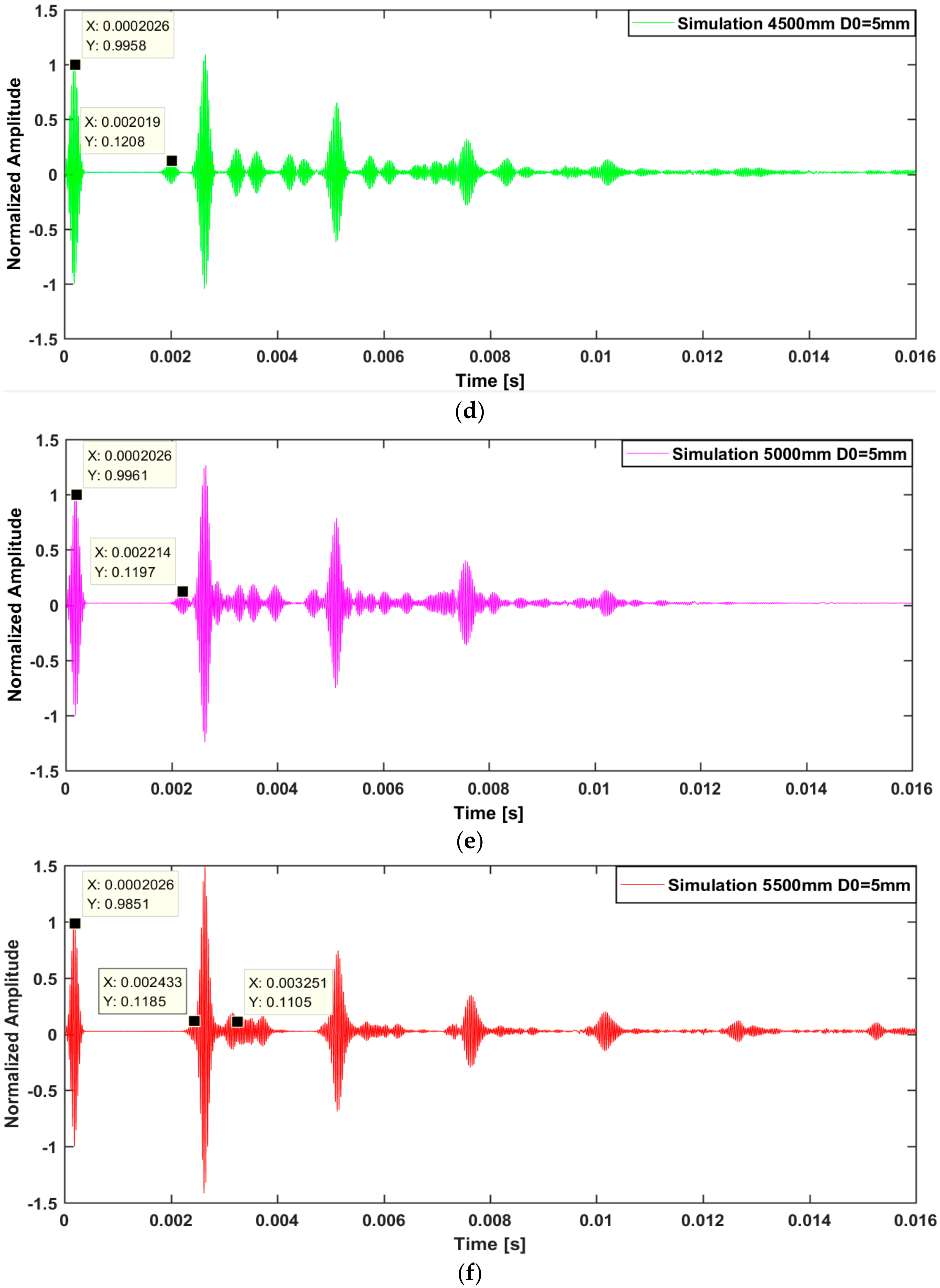
The flaw at 4000 mm (Figure 3c) can also be calculated in the same way so that its location can be determined using the reflected A0 mode and S0 mode waves. As shown in Figure 3d,e, the flaw at 4500 mm and 5000 mm can be only located by the S0 mode reflected pulse in the conventional inspection because the A0 mode pulse wave, which is in the superposition, is not in Interval I. As shown in Figure 3f, the times of the S0 mode and A0 mode flaw-reflected pulse waves in Interval I when D0 = 5 mm at 5500 mm are then calculated.

The appearance time of the S0 mode pulse wave $T_{S0}$ can be calculated using:

$$T_{S0}=0.0002026+(5.5-0.13)\times 2/C{g}_{S0}=0.0024333\hspace{0.17em}[\mathrm{s}]$$

(25)

The appearance time of the A0 mode pulse wave $T_{A0}$ can be calculated using:

$$T_{A0}=5.5/C{g}_{S0}+(5.5-0.13)/C{g}_{A0}=0.0032506\hspace{0.17em}[\mathrm{s}]$$

(26)

This analysis shows that, when the value of L increases along the x-direction and approaches the length of the terminal, the appearance time of the S0 mode flaw-reflected pulse wave and the A0 mode flaw-reflected pulse wave gradually approach the time of the first terminal reflection pulse wave, even then the appearance time of the A0 mode flaw-reflected pulse appears in the monitoring time Interval II at a given value of L. For the above simulation, at L = 5500 mm, the S0 mode flaw-reflected pulse wave is superimposed by the first terminal reflection pulse wave and the A0 mode flaw-reflected pulse wave is superimposed by these reflection pulse waves of the monitoring time Interval II.

In particular, the calculation (see Equation (26)) indirectly suggests that, in the monitoring Interval II, the highest reflected pulse is not the delay of the A0 mode flaw-reflected pulse in the conventional inspections, as shown in Figure 3f. Under ideal conditions, even without the interference of the signal trailing, the actual S0 or A0 mode flaw reflection pulses cannot be easily identified and the conventional detection method based on a single mode flaw-reflected pulse wave is invalid. For actual measurements, the trailing phenomenon of the pulse wave has to be considered. This is the state of the non-detection zone referred to in this study. It is known that the information of the flaw is superimposed by the first terminal reflection pulse wave and various types of reflection pulse waves in the monitoring time Interval II described in this section. In the following section, we observe the actual waveform of the ultrasonic pulse wave under the condition of the non-detection zone in an actual experiment.

3. Experimental Section

In this section, the experimental platform and the experimental results are presented and the occurrence of the non-detection zone in square steel inspections is briefly described.

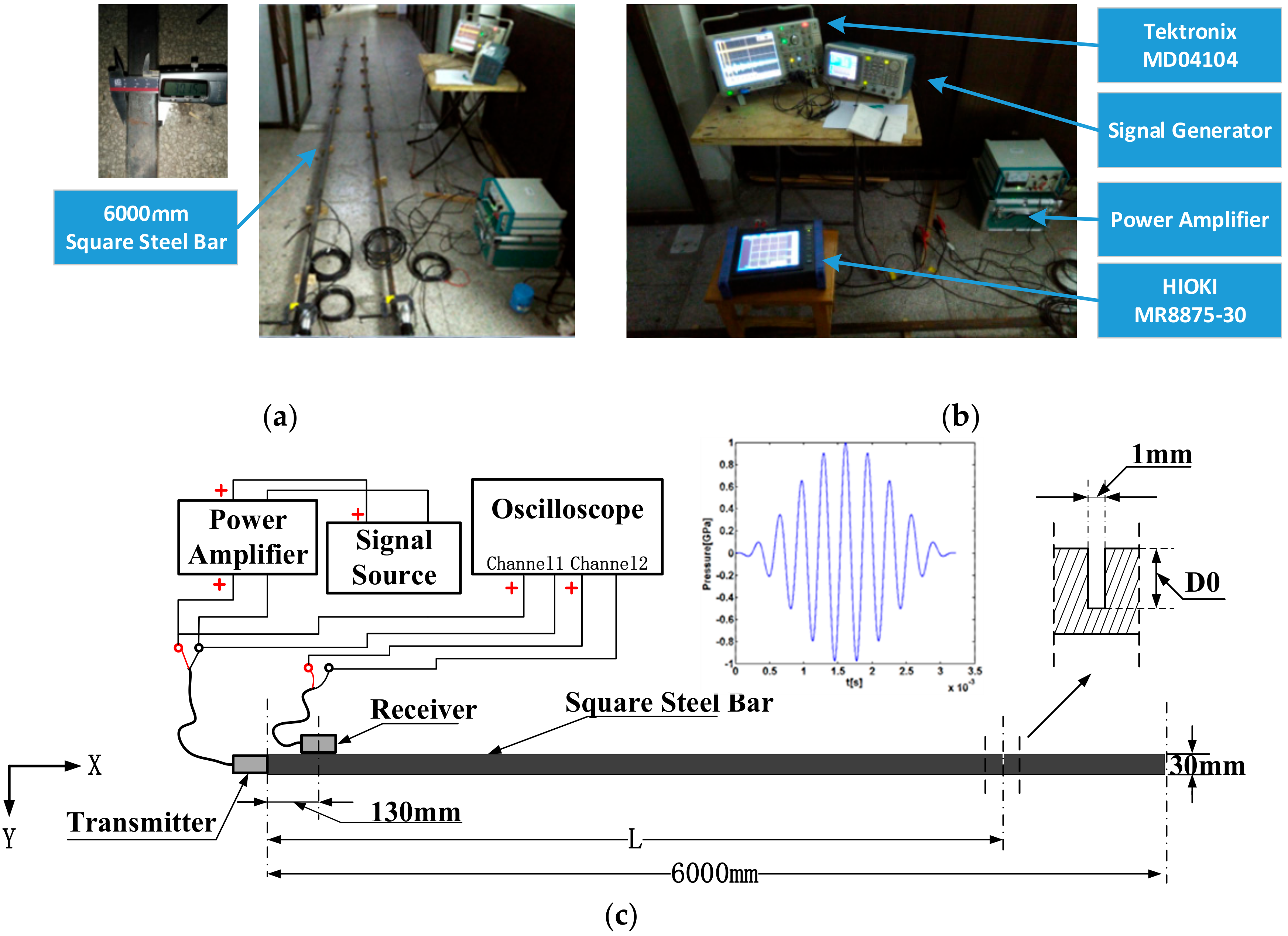
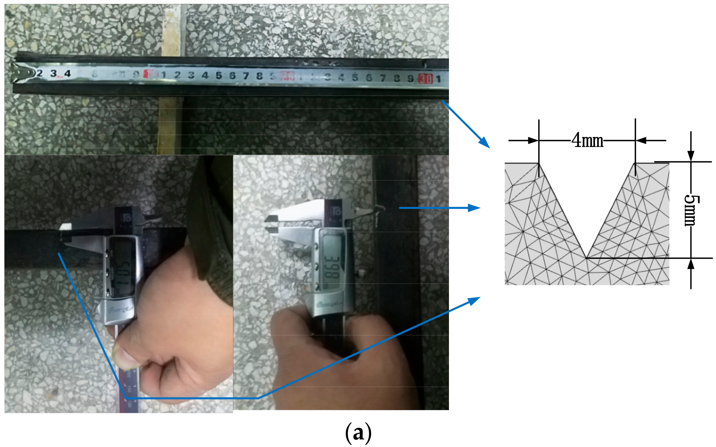
As shown in Figure 4a, a 30# (30 mm × 30 mm) square steel bar with a length of 6000 mm is used in this study; the length is sufficient to weaken the effect induced by signal trailing and facilitates the signal identification. These customized ultrasonic longitudinal-wave probes [21,22] with a central frequency of 30 kHz are installed using the dual-probe echo method. The signals are acquired and displayed using an oscilloscope (Tektronix MD04104) and the waves are recorded and the data are captured using a wave recorder (HIOKI MR8875-30), as shown in Figure 4b.

The Hamming pulse signal (10 cycles at the center frequency of $f_0=30\hspace{0.17em}[\mathrm{kHz}]$) is set by the signal source, which is loaded to the ultrasonic probe via a power amplifier. Transverse flaws with a width of 1 mm and a depth of 0~20 mm (D0) are created at a displacement L along the x-direction from the incident point. Because the thickness of the steel square bar is 30 mm and the length of the actual ultrasonic probe is 10 mm, a point (130.30) is selected as the measuring point. The excitation voltage amplitude is adjusted to acquire five reflected pulses and the waveforms of the reflected pulses are monitored in the time domain. Figure 4c shows the overall layout of the experimental platform.

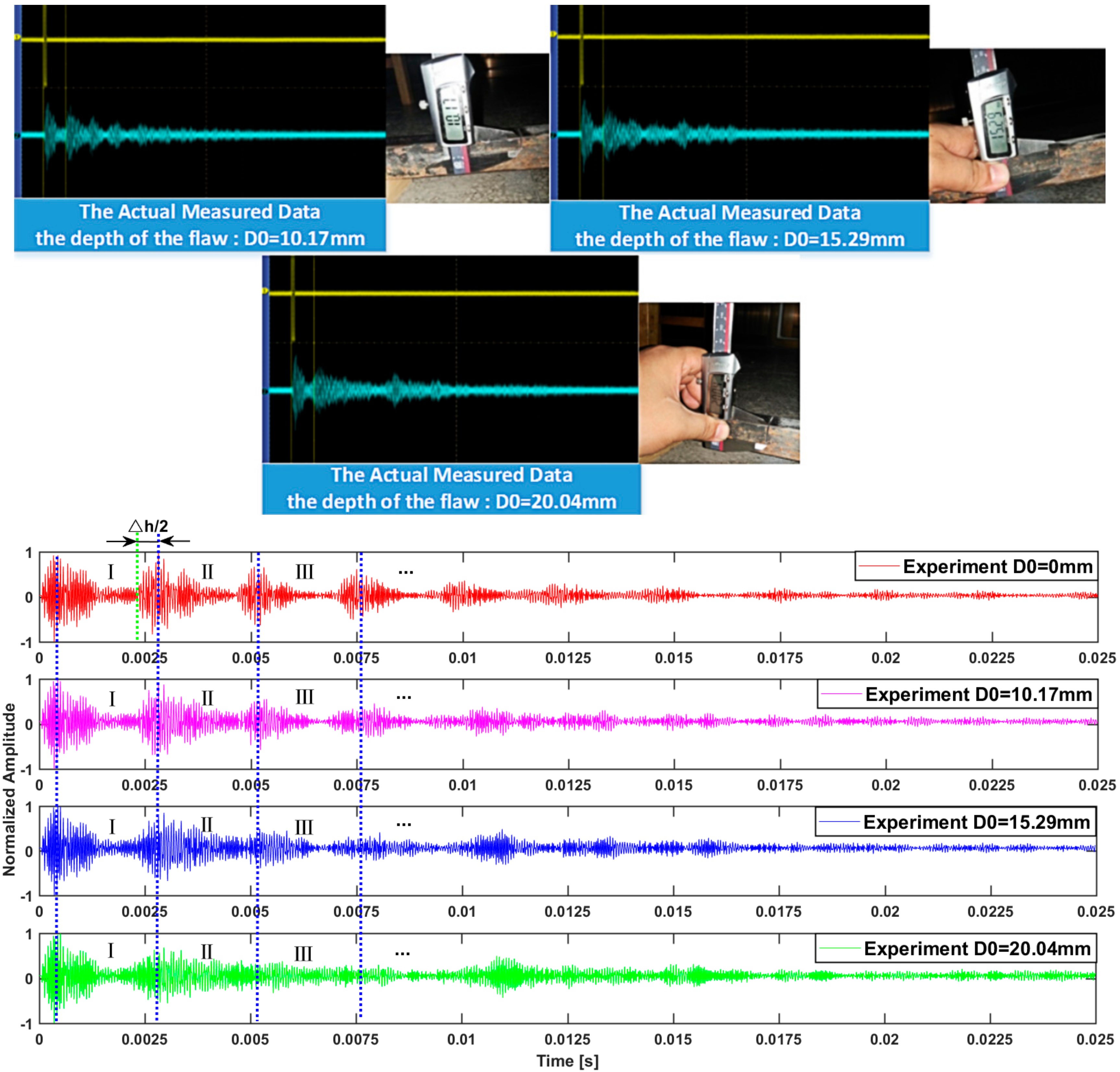
In a dual-probe echo long-distance inspection with the customized longitudinal-wave probe used in the experiment, the acquired reflected pulse wave of the transverse flaw occurs before reaching the first terminal; subsequently, the flaw can be located based on the modal wave velocity. However, both the experimental and the simulation results of the square steel inspection indicate that no reflected pulse is identified before the first terminal reflection pulse wave when the flaw is at a certain distance (L $\in$ (5300 mm, 6000 mm) from the excitation point. The experimental result at L = 5500 mm is used as an example (Figure 5). In the conventional monitoring Interval I, the reflected pulse wave with the flaw cannot be identified. According to the experimental data, even when the depth of the flaw (D0) reaches approximately 20 mm (i.e., the flaw represents almost 75% of the 30-mm thickness), no echo information is detected in the conventional monitoring Interval I. In actual measurements, when the ultrasonic pulse excitation ends, there are attenuation oscillations in the signal, namely the trailing phenomenon of the pulse wave. Many factors affect signal trailing, such as the manufacturing technique of the probes, the capacitance shock effect of the excitation circuit, and the sound absorption effect of the substrate. The trailing phenomenon is common in long-distance inspections with low-frequency ultrasonic guided waves [23,24]. In addition, the signal trailing compounds the difficulty of identifying the flaw-reflected pulse wave in the non-detection zone.

At L = 5500 mm, the S0 mode and A0 mode flaw-reflected pulse waves are superposed by the first terminal-reflected pulse wave, various types of reflection pulse waves in the monitoring time interval II, and the pulse signal trailing. Therefore, in a conventional inspection, the non-detection zone can be easily determined in the actual experiment. A similar experimental phenomenon can also occur in the ultrasonic flaw detection of long rod-like structures and cannot be ignored for NDT.

4. Analysis and Discussion

In this section, we analyze the range of the non-detection zone and the propagation characteristics of the ultrasonic guided wave in the non-detection zone using a simulation and experiments. Subsequently, we propose a feasible solution for the practical problems.

4.1. The Range of the Non-Detection Zone

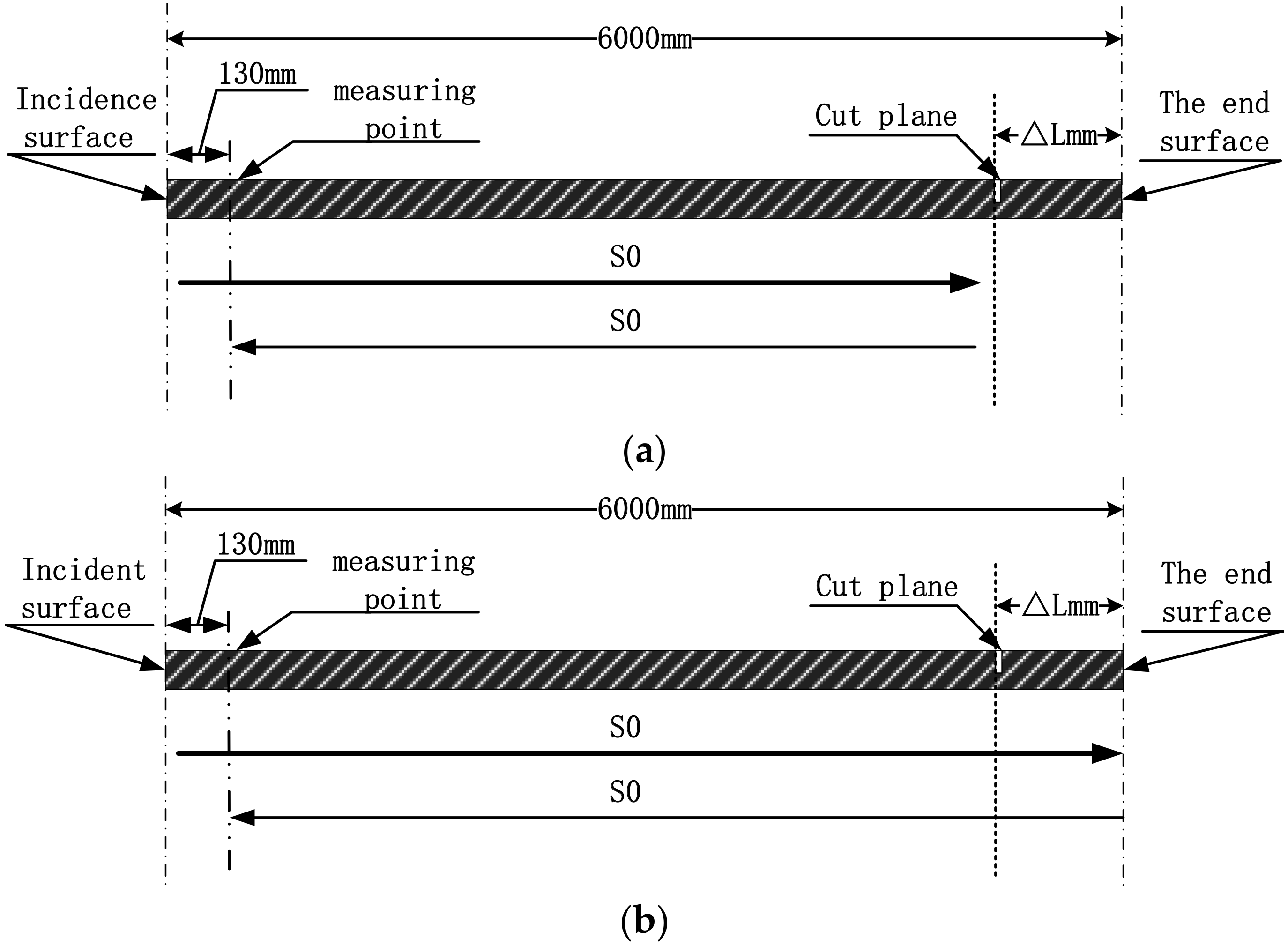
The range of the non-detection zone is a major concern in non-destructive inspections. Based on the analysis in Section 2.2, we used a dual-probe echo method for the location of the flaws and a low-frequency of the incident pulse. If the flaw is a certain distance from the terminal, the S0 mode flaw-reflected pulse is superposed by the first terminal-reflected pulse wave, while the A0 mode flaw-reflected pulse is superposed by the multiple reflected pulse wave and the pulse signal trailing in the monitoring interval II; as a result, the non-detection zone occurs. Therefore, the superposition time point of the S0 mode flaw-reflected pulse and the first terminal-reflected pulse wave can be considered as given the occurring conditions. Figure 6 shows the first terminal-reflected pulse wave and the S0 mode flaw-reflected wave.

Based on these occurring conditions, the range of the non-detection zone can be described as:

$$C{g}_{S0}\times (\Delta h/2)/2\ge \Delta L>0$$

(27)

where $C{g}_{S0}$ is related to the frequency-thickness product ($f\cdot d$) of the incident pulse wave, $\Delta L$ denotes the distance between the flaw and the terminal, $\Delta h$ denotes the pulse width of the first terminal-reflected pulse wave (Figure 3a and Figure 5), which is connected with the incident pulse wave and the self-characteristic of the customized longitudinal-wave probe, and $\Delta L$ denotes the distance between the flaw and the terminal reflection boundary. It should be noted that low-frequency ultrasound is normally used as the core frequency of the excitation pulse in long-distance ultrasonic guided wave inspections [24]. This has many advantages such as reducing the excitation mode number and extending the range of the long-distance detection [25]. However, the disadvantages cannot be ignored. One disadvantage is that the ultrasonic pulse width ($\Delta h$) is wider at a low frequency than at a high frequency. In addition, in a low-frequency ultrasonic guided wave propagated over a long distance [26], the width of the first terminal reflected pulse wave ($\Delta h$) increases because of the dispersion effect, thereby expanding the range of the non-detection zone.

The first terminal reflection pulse wave is the result of the overlap of the reflected pulse waves from the end surface and the incidence surface. The width of the first terminal reflection pulse wave ($\Delta h$) varies with the transmission distance. This is related to the measuring points, the detection distance, the characteristic of the probe, and so on. In this study, the range of the non-detection zone for the inspection of the 30# square steel bar with a length of 6000 mm is used as an example; the width of the first reflected pulse ($\Delta h$) is 0.000822 s in the actual experiment (Figure 5) and 0.0005371 s in the simulation (Figure 3a).

The governing equation for the Rayleigh-Lamb waves in a plate-like structure [1] for the symmetric mode is:

$$\tan (qd)/\tan (pd)=-4k^{2}pq/{(q^2-k^2)}^2$$

(28)

and for the anti-symmetric mode:

$$\tan (qd)/\tan (pd)=-{(q^2-k^2)}^2/4k^{2}pq$$

(29)

where $p^2=(\omega /c_L)-k^2$, $q^2=(\omega /c_T)-k^2$, the wave number $k=\omega /c_P$, the longitudinal wave velocity $c_L$, the shear velocity $c_T$, the phase velocity $c_P=(\omega /2\pi )\lambda$, the group velocity $C_g$ and the thickness of the plate is $d$.

The formula of the group velocity theory is:

$$C_g=d\omega /dk$$

(30)

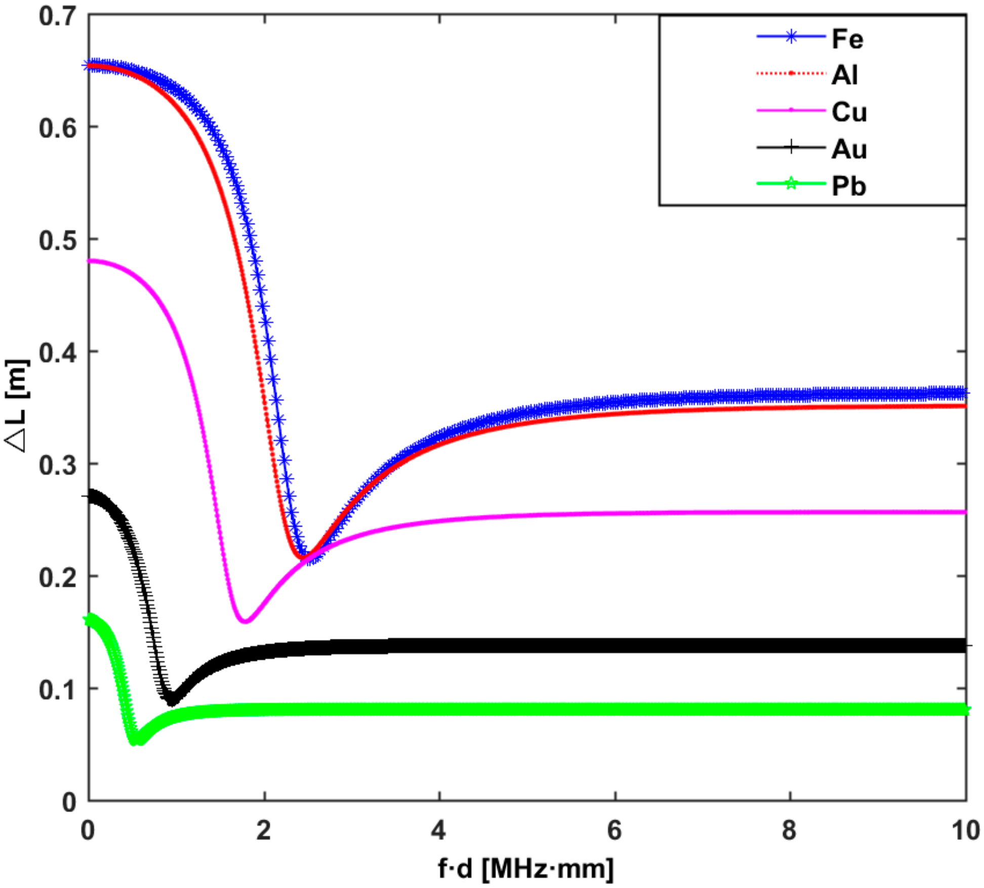
By using (Equations (28)–(30)) and selecting the material parameters for the iron plate and the curve of the S0 mode is calculated. According to the theoretical S0 wave group velocity ($C{g}_{S0}$) in the dispersion curve [27] and the width of the first terminal-reflected pulse ($\Delta h$) in the experiment, the curves of the non-detection zone range are calculated and are shown in Figure 7. For the ferrous material used in this study, for which the frequency-thickness product ($f\cdot d$) is 30 × 30 kHz·mm, the range of the corresponding non-detection zone ($\Delta L$) is 0.6390 m in the 6000 mm long steel square bar; This is basically coincident with the simulations. During the entire process, below a value of 2.5 MHz∙mm, the range of the non-detection zone decreases with the increase in the frequency-thickness product; when the frequency-thickness product is about 2.5 MHz∙mm, the minimum length of the non-detection zone is 0.2 m. In the range of 2.5 MHz∙mm to 5.0 MHz∙mm, the range of the non-detection zone increases with the increase in the frequency-thickness product. When the ultrasonic guided wave has a frequency-thickness product of 5.0 MHz∙mm, the range of the non-detection zone varies slightly. In an actual long-distance ultrasonic guided wave propagation process, the range of the non-detection zone expands with the widening of the first terminal-reflected pulse wave, which is a new reference factor to be considered. Similarly, the simulations are conducted using different materials [1] and the other conditions remain unchanged, as the simulated non-detection zone shows in Figure 7. The materials have different properties, resulting in the increase in the minimum length of the non-detection zone. Because the minimization of the non-detection zone is desirable, alloying may present a solution in the low-frequency range.

Although the flaw’s pulse signal is lost in monitoring Interval I, the reflected pulses carrying the flaw information can still be detected in other monitoring intervals, thus allowing the determination of the flaw’s location. By analyzing the simulation results that satisfy the conditions for the appearance of the non-detection zone, it can be found that the overall pulse waveform exhibits apparent variations in monitoring Interval II.

4.2. Characteristics of the Reflected Pulse Wave in Monitoring Interval II

This study attempts to locate the flaw in the non-detection zone using the reflected pulse wave in monitoring Interval I and monitoring Interval II based on a simulation and experimental results. The primary reasons are listed below. Firstly, the amplitude of the reflected pulse in the monitoring Interval II exceeds that encountered in the following monitoring intervals. Secondly, because the existence of the flaw, an increasing number of derivative pulse waves will occur as the propagation time increases; the condition of the pulse wave superposition is simpler in monitoring Interval II than in the following monitoring Intervals. Therefore, we used the square steel bar with a length of 6000 mm as an example and analyzed the variation of the reflected pulse waveform in monitoring Interval II.

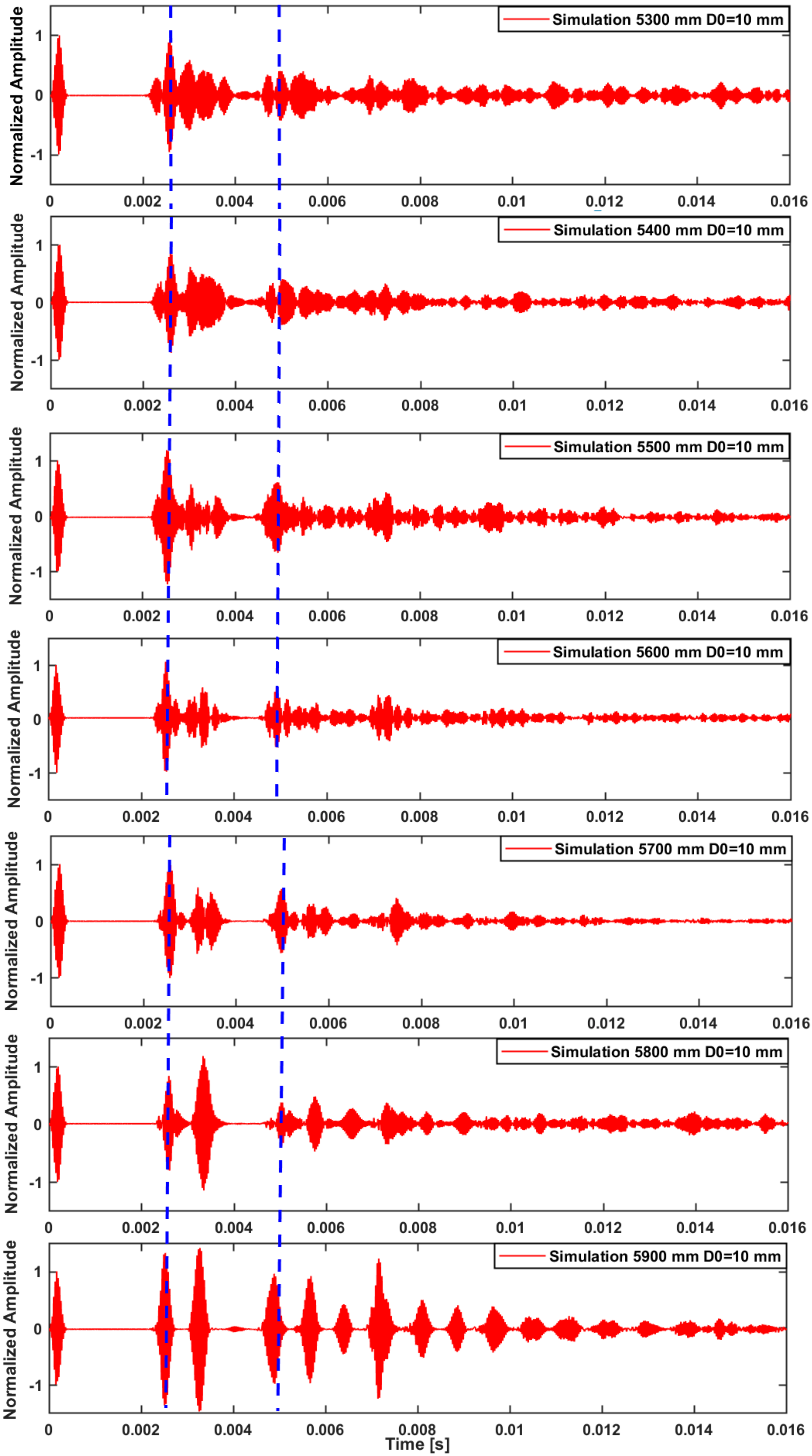
Due to the variation of the pulse width of the terminal-reflected pulse wave and the waveform superposition in the actual experiments, the non-detection zone is observed in advance when L = 5300 mm. Therefore, this study focused on the simulation range of [5300 mm, 5900 mm] with D0 = 10 mm and the simulation interval of 100 mm. The analysis indicates that the amplitude changed with the changes in D0, leading to new changes in the envelope superposition of the incident pulse in Interval II and especially in the superposition of the amplitudes. We used D0 = 10 mm as an example of the representative and significant waveform change; other values of D0 can also be used for the same method.

Figure 8 shows the simulation results. It can be observed that, as the flaw location (L) changes, the amplitude of the superposed pulse wave exhibits complex changes in the time domain, especially in Interval II. Moreover, as the flaw location (L) changes, the superposition envelope of multiple reflected pulses changes significantly in monitoring Interval II, i.e., both of these factors showed a one-to-one correspondence. Within the monitoring Interval II, there exists multiple reflected wave energy; at first, at around L = 5300~5500 mm, the highest reflected pulse gradually moves backward; at around L = 5600~5700 mm, the two highest reflected pulses appear in adjacent time-domains; at around L = 5800~5900 mm, the flaw position is close to the terminal, the energy gradually becomes concentrated, and the amplitudes of these flaw-reflected pulse waves are significantly higher than the amplitude of the first terminal reflected pulse wave for the two conditions. Therefore, we attempted to use the above-mentioned correspondence and estimated the location of the flaw through reverse deduction based on envelope comparison.

4.3. Approximation Based on Envelope Comparison

Although the reflected pulses show complex superposition patterns in Interval II, the propagation speed of the fundamental mode remains relatively stable and the superposition state varies correspondingly as the flaw location L changes along the x-direction. If the energy of the excitation pulse signal, the flaw location L, and D0 were fixed, the propagation energy would attenuate. Compared with the condition without any flaws, the amplitude of the pulse overall decreases but the amplitude of the pulse reflected by the flaw increases. The difference in the envelope between these two different conditions (with and without the flaw) of the pulse waves can be used to identify the reflected pulse.

Because the ultrasonic reflected pulse wave from the flaws located in monitoring Interval I is invalid, we decided to use the envelope wave of the pulse that is extended to monitoring Interval II to locate the flaws. To resolve the interference problem caused by the trailing of the actual experimental data and the unexpectedly generated waves, firstly, we use the envelope of the waveforms of two areas (for example, D0 = 0 mm and D0 = 10 mm) in the simulation and in the experiment and calculate the difference in the envelope amplitude of the two areas; these are used as basic data for comparison.

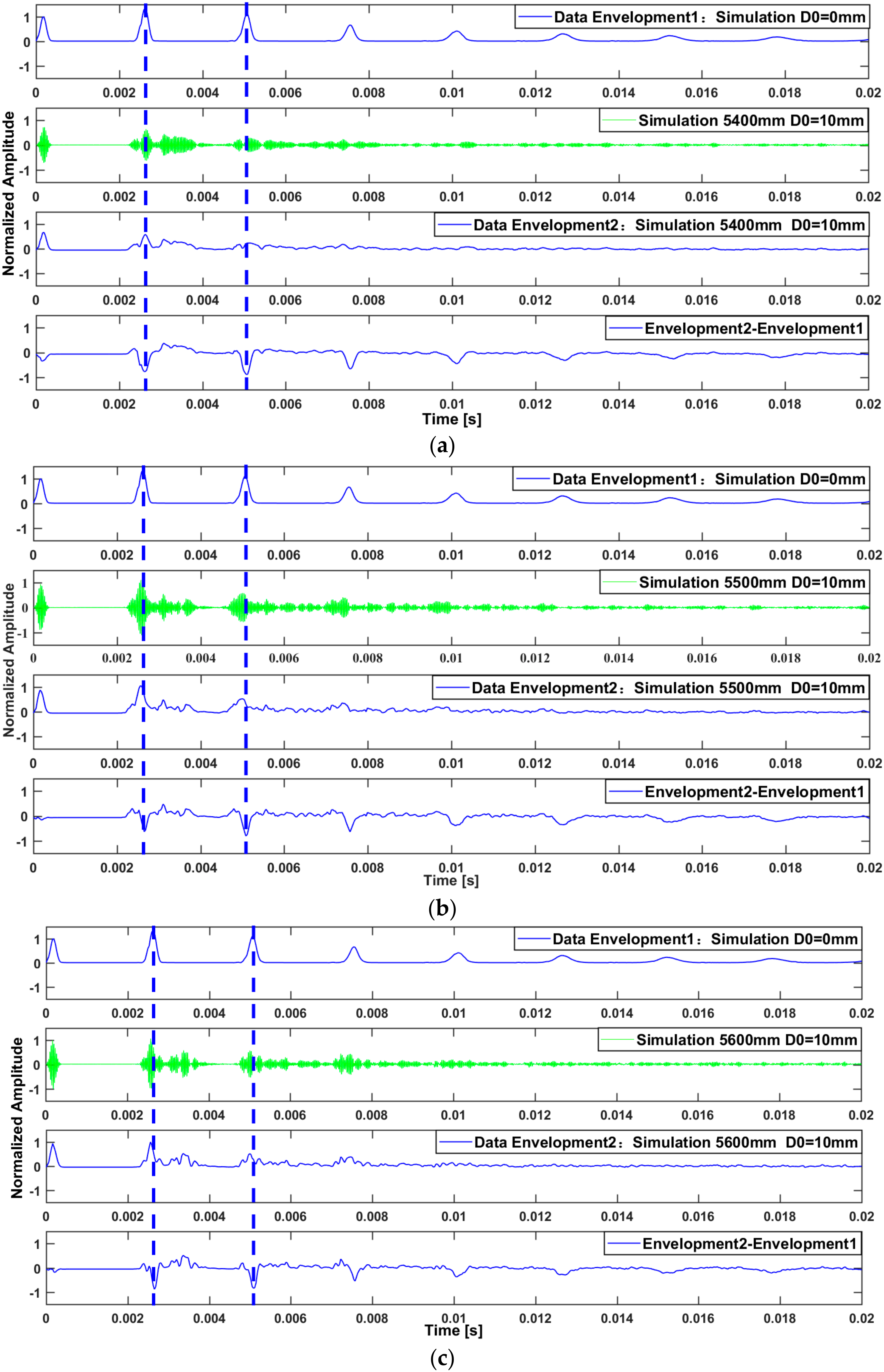
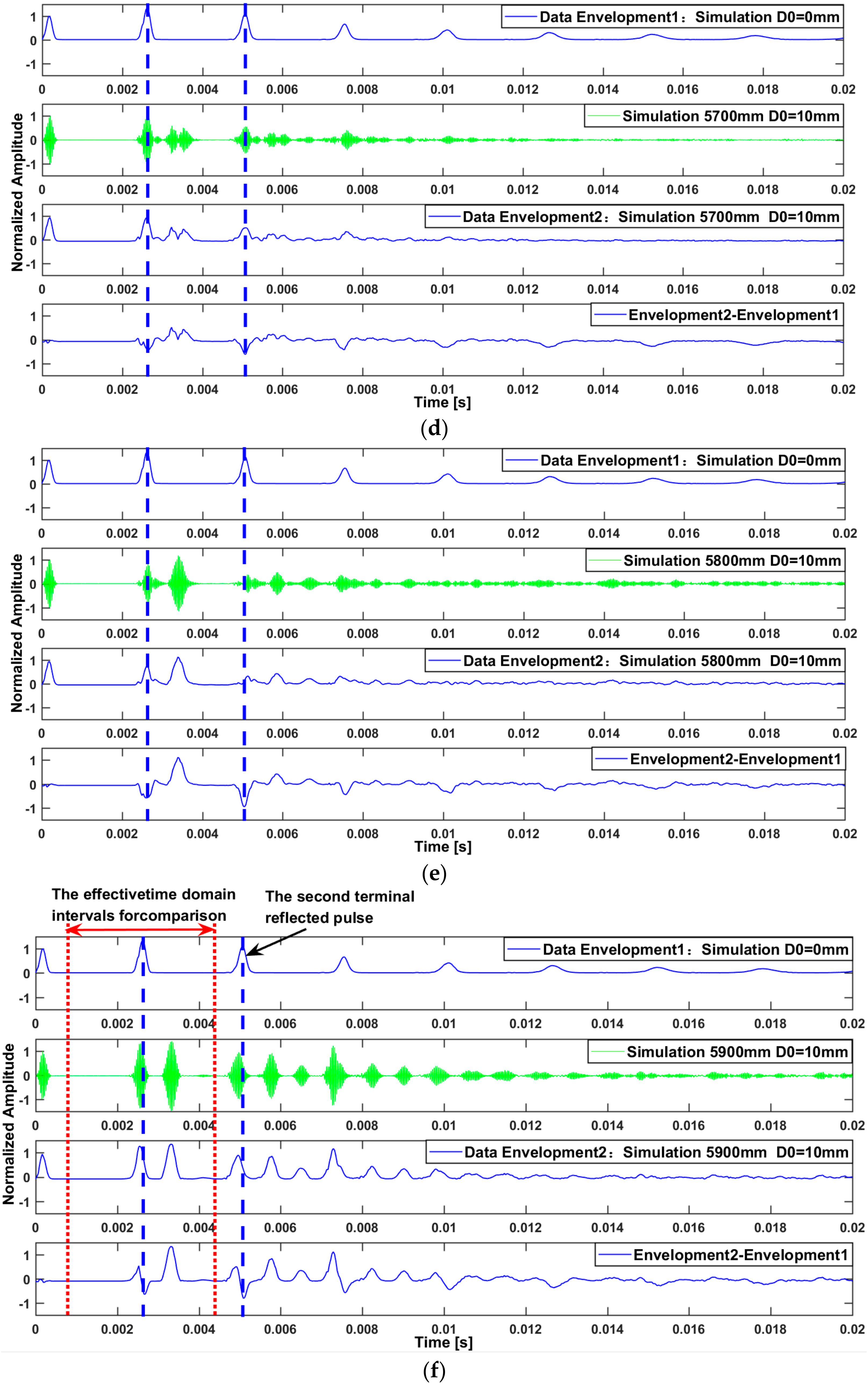
Firstly, by observing these envelopes shown in Figure 9a–f, a coarse division of the flaw areas is proposed based on the analysis in Section 4.2.

• Situation 1: in the actual experimental envelope during monitoring Interval II, the reflected pulse with only one envelope amplitude that is larger than the amplitude of the terminal reflected pulse wave is categorized into a zone ranging from L = 5800 mm to L = 5900 mm;
• Situation 2: the reflected pulses with two similar highest envelope amplitudes are categorized into a zone ranging from L = 5600 mm to L = 5700 mm;
• Situation 3: the remaining flaw detection pulses with different amplitudes are categorized into a zone from L = 5400 mm to L = 5500 mm.

Secondly, we selected the effective time domain intervals for comparison (from 7.649 × 10⁻⁴ s to 4.653 × 10⁻³ s intervals within the monitoring Intervals I and II) to avoid the interference caused by the trailing of the incident pulse and the second terminal-reflected pulse wave, as shown in Figure 9f.

Thirdly, the envelope theory (ET) is known as an auxiliary field method [28,29]; therefore, we could use this convenient method for the wave comparison between the simulation and the measurements. The envelope correlation algorithm is applied to compute the maximum correlation coefficient in order to choose the most similar envelope waveforms in a quantitative approach and locate the flaws.

The discretization cross-correlation function can be represented as follows:

$$R_{se}(k)={\displaystyle \sum _{n=0}^{N-1}s(n)e(n-k)} k=0,1,2,\cdots ,M-1$$

(31)

where $R_{se}(k)$ denotes the correlation function for the simulation data $s(n)$ and the experimental data $e(n)$. $N$ is the cumulative average number and $k$ is the time-lapse sequence number, $M$ is a positive integer. The formula for the envelope correlation is expressed as follows:

$$\rho =R_{se}(0)/\sqrt{{\displaystyle \sum _{n=0}^{N-1}{s}^2(n){\displaystyle \sum _{n=0}^{N-1}{e}^2(n)}}}$$

(32)

The scan comparisons are not required ($k=0$) in Equation (31). The envelope correlation coefficient ($\rho$) of the experimental data and the simulation data are obtained using Equation (32), and the envelope whose simulation data is closest to the experimental data envelope is selected as the indicator for locating the corresponding flaw.

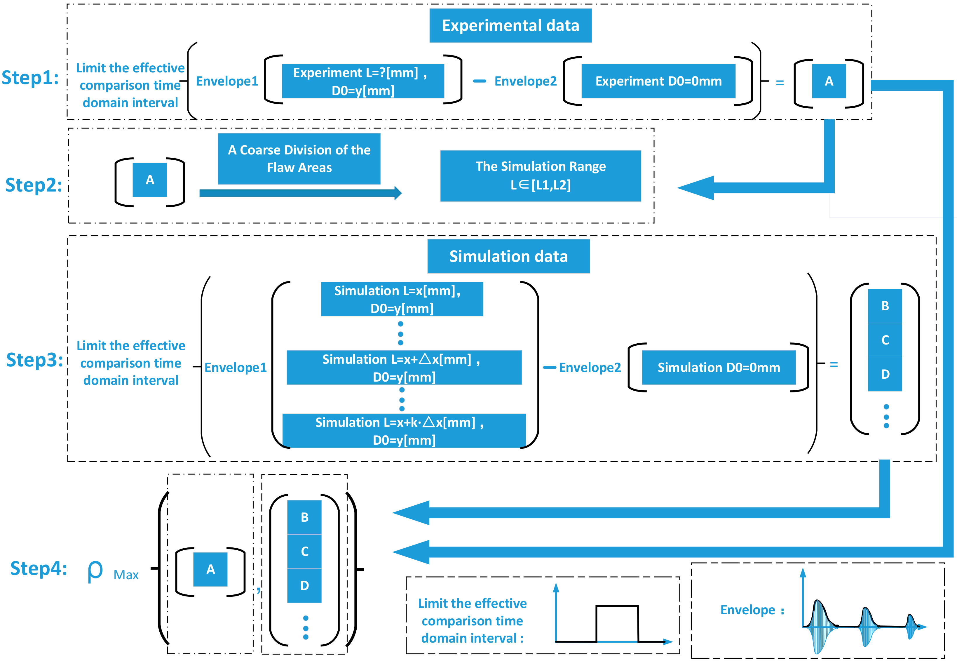
From the above analysis, the approximation is based on the inverse comparison with the simulation envelope in the non-detection zone. As shown in Figure 10, the main steps are as follows:

Data pre-processing: we prepared the envelope data in the experiment and the simulation without the flaw. The experimental data can be replaced by the experimental data of a similar square steel bar without flaws in practical measurements. For the simulation data, we can use D0 = 0 mm.

• Step 1: The experimental data with the flaw obtained in the non-detection zone are processed using the envelope calculation and we subtract the envelope of the experimental data without the flaw to reduce the effect of the signal trailing. Then the result of the envelope is extracted in the effective comparison interval (from 7.649 × 10⁻⁴ s to 4.653 × 10⁻³ s).
• Step 2: Based on the obtained experimental envelope (Envelopment 2–Envelopment 1), the simulation range (L $\in$ [L₁, L₂]) is selected according to the rough classification described in Section 4.3 to reduce the computation cost.
• Step 3: According to the comparison requirements, the variable value of L is selected in the appropriate range (L₁ mm ≤ L₁ + kΔx ≤ L₂ mm, Δx = 100 mm, k $\in$ N), the depth of the flaw (y) in the experiment is selected as the value of D0 in the simulation (0 mm ≤ D0 = y < 30 mm), and the simulation results have been processed using the envelope calculations respectively. For every simulation envelope, the envelope of the simulation without the flaw (D0 = 0 mm) is subtracted. Then the results of these envelopes are extracted in the comparison interval as a series of comparisons.
• Step 4: The correlation coefficients between the experimental envelope data from Step 1 and every simulation envelope data from Step 3 are determined and the result returns the maximum correlation coefficient $\rho$; subsequently, the estimated position of the flaw (L) is determined according to the reverse correspondence.

Final data processing: By changing the value of Δx, a similar approximation is used near the initial estimated value of L to approximate the real value of L in a further simulation.

4.4. Experimental Validation

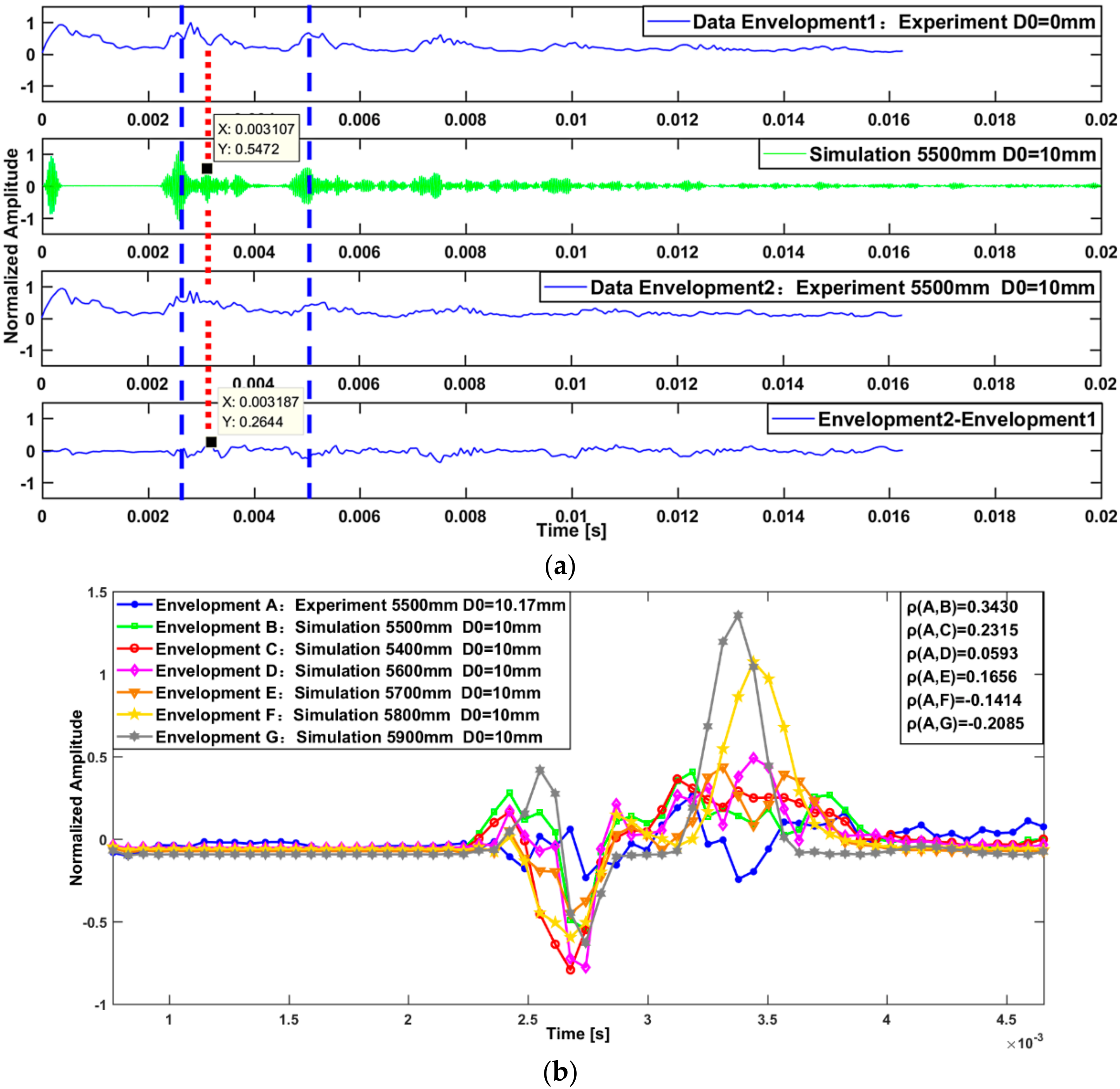
In order to localize the flaw in the non-detection zone, the different envelopes of the simulated envelope waveforms (Envelopment 2–Envelopment 1) are used as the evaluation standard to compare with those of the experimental data. This section describes the validation of the experiment. In order to depict the validation results, instead of strictly following the steps mentioned in Section 4.3, the preliminary classification in Step 2 was omitted. The variable value of L is selected from an appropriate range (L₁ = 5400 mm, L₂ = 5900 mm) in the simulation. D0 = 10 mm is used as an example of the experimental data to determine the location of the flaw (L).

Figure 11a shows the experimental pulse waveform of the square steel bar without the flaw (D0 = 0 mm) and the experimental and simulated pulse waveforms of the square steel bar with the flaw (D0 = 10 mm). Using the envelope calculation, it can be observed that the envelope waveform in monitoring Interval II reduces the interference of the signal trailing in the experiments. Compared with the simulation data, it is evident that the peak points of the difference envelopes in the experiment are consistent, as shown in the red dotted line. The time relative deviation ${\sigma }_1$ can be calculated by:

$${\sigma }_1=(0.003187-0.003107)/0.003187=2.5101\%$$

(33)

The flaw’s reflected information that is hidden and the superposition envelope of the flaw-reflected pulse in the trailing are extracted (Envelopment 2–Envelopment 1).

Subsequently, the results of the different envelopes (Envelopment 2–Envelopment 1) in the simulation and the experiment are extracted in the comparison interval, as shown in Figure 11b. The correlation coefficients ($\rho$) of the experimental data and the different simulation data are determined. Because the simulated envelope waveform is used as the evaluation standard, the noise introduced by the real application cannot be eliminated by the correlation algorithm; therefore, the correlation coefficient is relatively low. However, we can still determine that the correlation coefficient, which is negative, should be discarded in the range from L = 5800 mm to L = 5900 mm; in the range from L = 5600 mm to L = 5700 mm, the envelopes of the waveform are not well matched. However, in the range from L = 5400 mm to L = 5500 mm, the approximated simulation waveforms in the flaw area (L = 5500 mm) have a significant correlation coefficient of 0.3430; therefore, L = 5500 mm is selected as the estimated value of the location of the flaw. If these calculating steps are strictly carried out according to the solution in the previous section, based on the preliminary rough classification, it is found that the actual measurement data range from L = 5400 mm to L = 5500 mm and we can obtain similar results rapidly to approximate the real value of L in further simulations.

Therefore, the flaw in the non-detection zone can be identified using the inverse correspondence. Using an equivalent mode and approximation algorithms, this methodology provides estimations of the locations of flaws relatively accurately.

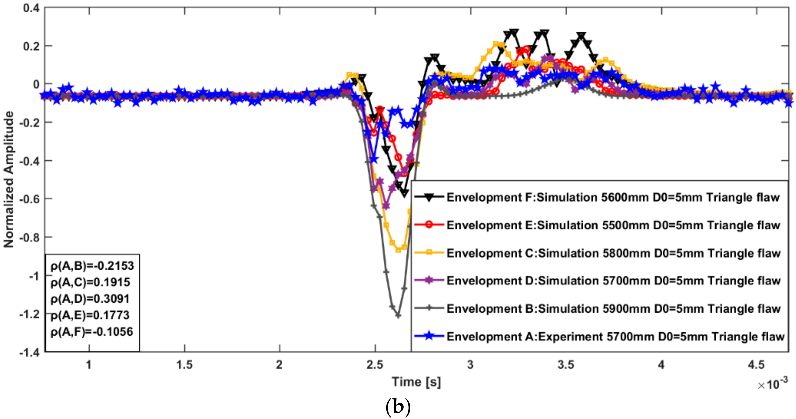
Based on the analysis in Section 2.1.1, when the equivalent plate thickness (d) is constant, as long as the frequency is below the cutoff frequency of A1 and S1, the excitation frequency in this range can be used for low-frequency ultrasound mode selection. For example, the proposed analysis is applicable to the ultrasonic probe core frequency range of 20–60 kHz low-frequency ultrasonic guided wave detection. The concept of detecting flaws using simulations also applies to different types of flaws. In this study, we extended the analysis to a triangular flaw. This approach also resulted in a similar positioning effect. When $f\cdot d$ is known, the modal phase velocity and the group velocity basically remain unchanged, whereas there is a one-to-one correspondence between the type of the reflected pulse wave and the location of the flaw. Therefore, in this study, we use a triangular flaw (40 kHz, D0 = 5 mm, L = 5700 mm) as another example.

Based on the data analysis shown in Figure 12, we can obtain a similar conclusion; the flaw area (L = 5700 mm) has a significant correlation coefficient (ρ) of 0.3091. Therefore, L = 5700 mm is then selected as the estimated value of L (the location of the flaw). The solution remains valid, but the characteristics of the waveform superposition have changed, which can be used to identify the triangle type of the flaw.

The relevant analysis and the solution presented in this paper are still valid for low-frequency ultrasonic guided wave detection in a rod-like structure medium. We can also obtain a similar conclusion for the non-detection zone problem for a rail structure. For example, a rail experiment using 60 kHz as the actual measurement frequency was conducted by Rose [9]. Although the experiment used different excitation pulse waveforms, which were affected by other derived modes wave and pulse trailing, the superimposed reflected pulse waveform obtained in the second monitoring time domain and the peak value was far higher than the peak value of the first reflected pulse; this result is very similar to the results of the characteristic analysis in this study.

5. Conclusions

Previous studies have provided no clear statements or solutions regarding the non-detection zone in low-frequency ultrasonic guided waves. However, the existence of the non-detection zone cannot be ignored in NDT. In this study, we located the non-detection zone in long-distance conventional ultrasonic guided wave inspections of a square steel bar and investigated the reasons and conditions for the appearance of the non-detection zone through simulations. Further, by analyzing the characteristics of the simulated pulse wave when the non-detection zone appears, the range of the non-detection zone and a solution are proposed. The simulation envelope is used for a relative comparison; by suppressing the interference of the ultrasonic signal trailing using the envelope calculation, the flaw is located by a comparison with the simulation results of the multi-pulse superimposed envelope in the extended time domain (the monitoring time Intervals I and II). The simulation results are verified with actual measurements. The results of this study provide a feasible solution for locating the non-detection zone and serve as a powerful supplement for conventional long-distance ultrasonic guided wave inspections. This type of non-detection zone can also occur in the ultrasonic flaw detection of long rod-like structures; therefore, this study has certain applicability and practical significance for other structures. However, due to the influence of actual field factors on the actual detection of the pulse energy loss, the amplitude deviation between the equivalent simulation and the actual measurement is large in this study and is not conducive to the prediction of the depth (D0) of the flaw. For this reason, it is necessary to improve the approximate model of the low-frequency ultrasonic guided wave and the estimation of various types of flaws to provide a new approach that is widely applicable.

References

- Rose, J.L. Ultrasonic Guided Waves in Solid Media, 1st ed.; Cambridge University Press: New York, NY, USA, 2014; ISBN 978-110-70489-59. [Google Scholar]
- Rose, J.L. Ultrasonic Waves in Solid Media, 1st ed.; Cambridge University Press: New York, NY, USA, 1999; ISBN 0521640431. [Google Scholar]
- Ai, C.Y.; Li, J.; Liu, Y.; Ni, T. Ultrasonic Test Theory and Technology for Multilayered Bonding Structure, 1st ed.; National Defence Industry Press: Beijing, China, 2014; ISBN 978-711-80958-07. [Google Scholar]
- Verma, B.; Mishra, T.K.; Balasubramaniam, K.; Rajagopal, P. Interaction of low-frequency axisymmetric ultrasonic guided waves with bends in pipes of arbitrary bend angle and general bend radius. Ultrasonics 2014, 54, 801–808. [Google Scholar] [CrossRef] [PubMed]
- Ryue, J.; Thompson, D.J.; White, P.R.; Thompson, D.R. Decay rates of propagating waves in railway tracks at high frequencies. J. Sound Vib. 2009, 320, 955–976. [Google Scholar] [CrossRef]
- Gravenkamp, H.; Prager, J.; Saputra, A.A.; Song, C. The simulation of lamb waves in a cracked plate using the scaled boundary finite element method. J. Acoust. Soc. Am. 2012, 132, 1358–1367. [Google Scholar] [CrossRef] [PubMed]
- Bartoli, I.; Scalea, F.L.D.; Fateh, M.; Viola, E. Modeling guided wave propagation with application to the long-range defect detection in railroad tracks. NDT E Int. 2005, 38, 325–334. [Google Scholar] [CrossRef]
- Campos-Castellanos, C.; Gharaibeh, Y.; Mudge, P.; Kappatos, V. In the application of long range ultrasonic testing (LRUT) for examination of hard to access areas on railway tracks. Railw. Cond. Monit. Non-Destr. Test. 2012, 1–7. [Google Scholar] [CrossRef]
- Rose, J.L.; Avioli, M.J.; Mudge, P.; Sanderson, R. Guided wave inspection potential of defects in rail. NDT E Int. 2004, 37, 153–161. [Google Scholar] [CrossRef]
- Wu, J.; Wang, Y.; Zhang, W.; Nie, Z.; Lin, R.; Ma, H. Defect detection of pipes using Lyapunov dimension of Duffing oscillator based on ultrasonic guided waves. Mech. Syst. Signal Proc. 2016, 82, 130–147. [Google Scholar] [CrossRef]
- Yao, W.; Sheng, F.; Wei, X.; Zhang, L.; Yang, Y. Propagation characteristics of ultrasonic guided waves in continuously welded rail. Mod. Phys. Lett. B 2017, 1740075. [Google Scholar] [CrossRef]
- Su, Z.; Ye, L.; Lu, Y. Guided lamb waves for identification of damage in composite structures: A review. J. Sound Vib. 2006, 295, 753–780. [Google Scholar] [CrossRef]
- Fateri, S.; Lowe, P.S.; Engineer, B.; Boulgouris, N.V. Investigation of ultrasonic guided waves interacting with piezoelectric transducers. IEEE Sens. J. 2015, 15, 4319–4328. [Google Scholar] [CrossRef]
- Mirahmadi, S.J.; Honarvar, F. Application of signal processing techniques to ultrasonic testing of plates by lamb wave mode. NDT E Int. 2011, 44, 131–137. [Google Scholar] [CrossRef]
- Pai, P.F.; Deng, H.; Sundaresan, M.J. Time-frequency characterization of lamb waves for material evaluation and damage inspection of plates. Mech. Syst. Signal Proc. 2015, 62–63, 183–206. [Google Scholar] [CrossRef]
- Deng, Q.T.; Yang, Z.C. Scattering of S0 lamb mode in plate with multiple damages. Appl. Math. Model. 2011, 35, 550–562. [Google Scholar] [CrossRef]
- Wan, X.; Tse, P.W.; Chen, J.; Xu, G.; Zhang, Q. Second harmonic reflection and transmission from primary s0 mode lamb wave interacting with a localized microscale damage in a plate: A numerical perspective. Ultrasonics 2017, 82, 57–71. [Google Scholar] [CrossRef] [PubMed]
- Glushkov, E.; Glushkova, N.; Eremin, A.; Giurgiutiu, V. Low-cost simulation of guided wave propagation in notched plate-like structures. J. Sound Vib. 2015, 352, 80–91. [Google Scholar] [CrossRef]
- Rucka, M. Experimental and numerical study on damage detection in an l-joint using guided wave propagation. J. Sound Vib. 2010, 329, 1760–1779. [Google Scholar] [CrossRef]
- Le, C.E.; Castaings, M.; Hosten, B. The interaction of the s0 lamb mode with vertical cracks in an aluminium plate. Ultrasonics 2002, 40, 187–192. [Google Scholar] [CrossRef]
- Yang, Y.; Wei, X.; Zhang, L.; Yao, W. The effect of electrical impedance matching on the electromechanical characteristics of sandwiched piezoelectric ultrasonic transducers. Sensors 2017, 17, 2832. [Google Scholar] [CrossRef] [PubMed]
- Wei, X.; Yang, Y.; Yao, W.; Zhang, L. Pspice modeling of a sandwich piezoelectric ceramic ultrasonic transducer in longitudinal vibration. Sensors 2017, 17, 2253. [Google Scholar] [CrossRef] [PubMed]
- Zhao, Y.; Li, F.; Cao, P.; Liu, Y.; Zhang, J.; Fu, S.; Zhang, J.; Hu, N. Generation mechanism of nonlinear ultrasonic lamb waves in thin plates with randomly distributed micro-cracks. Ultrasonics 2017, 79, 60–67. [Google Scholar] [CrossRef] [PubMed]
- Loveday, P.W. Simulation of piezoelectric excitation of guided waves using waveguide finite elements. IEEE Trans. Ultrason. Ferroelectr. Freq. Control 2008, 55, 2038. [Google Scholar] [CrossRef] [PubMed]
- Ryue, J.; Thompson, D.J.; White, P.R.; Thompson, D.R. Investigations of propagating wave types in railway tracks at high frequencies. J. Sound Vib. 2008, 315, 157–175. [Google Scholar] [CrossRef]
- Zhang, Y.; Li, D.; Zhou, Z. Time reversal method for guided waves with multimode and multipath on corrosion defect detection in wire. Appl. Sci. 2017, 7, 424. [Google Scholar] [CrossRef]
- Zhang, H.Y.; Xu, J.; Ma, S.W.; Ta, D.A. The high-frequency scattering of the s0 lamb mode by a circular blind hole in a plate. Phys. Procedia 2015, 70, 455–458. [Google Scholar] [CrossRef]
- Santacruz, J.; Tardón, L.; Barbancho, I.; Barbancho, A. Spectral envelope transformation in singing voice for advanced pitch shifting. Appl. Sci. 2016, 6, 368. [Google Scholar] [CrossRef]
- Semay, C. The hellmann–feynman theorem, the comparison theorem, and the envelope theory. Results Phys. 2015, 5, 322–323. [Google Scholar] [CrossRef]
Figure 1.
The equivalent model in low-frequency (a) The equivalent model of low-frequency ultrasonic guided wave in a square steel bar; (b) Low-frequency phase velocities of S0 and A0 modes provided by the beam, plate and elastic layer models.
Figure 2.
The simulation settings.
Figure 3.
Waveforms of the reflected pulses in the simulation, (a) D0 = 0 mm; (b) D0 = 5 mm, L = 3500 mm; (c) D0 = 5 mm, L = 4000 mm; (d) D0 = 5 mm, L = 4500 mm; (e) D0 = 5 mm, L = 5000 mm; (f) D0 = 5 mm, L = 5500 mm.
Figure 4.
Establishment of the experimental platform (a) square steel bar with a length of 6000 mm; (b) picture of experimental instruments; (c) the diagram of the establishment of experimental platform.
Figure 5.
The reflected pulse waves with different values of D0 at 5500 mm.
Figure 6.
Schematic of the distance covered by the S0 mode pulse wave in (a) the first terminal-reflected pulse wave and (b) the flaw-reflected pulse wave in Interval I.
Figure 7.
Curves of the non-detection zone ranges for different materials.
Figure 8.
Simulated waveforms of the square steel bar with a length of 6000 mm at L ∈ [5300 mm, 5900 mm].
Figure 9.
Envelope calculation results of the pulse wave at different locations of flaw: (a) L = 5400 mm D0 = 10 mm (b) L = 5500 mm D0 = 10 mm (c) L = 5600 mm D0 = 10 mm (d) L = 5700 mm D0 = 10 mm (e) L = 5800 mm D0 = 10 mm (f) L = 5900 mm D0 = 10 mm.
Figure 10.
The schematic diagram of the envelope approximation method.
Figure 11.
Location of the flaw through the envelope approximation method: (a) The envelope of experimental data processing (b) The comparison of multiple envelopes in the effective comparison interval.
Figure 12.
Location of a triangle flaw. (a) The triangle type of the flaw on the steel square bar; (b) The comparison of multiple envelopes in the effective comparison interval for the triangle flaw.
© 2018 by the authors. Licensee MDPI, Basel, Switzerland. This article is an open access article distributed under the terms and conditions of the Creative Commons Attribution (CC BY) license (http://creativecommons.org/licenses/by/4.0/).
Share and Cite
MDPI and ACS Style
Zhang, L.; Yang, Y.; Wei, X.; Yao, W. The Study of Non-Detection Zones in Conventional Long-Distance Ultrasonic Guided Wave Inspection on Square Steel Bars. Appl. Sci. 2018, 8, 129. https://doi.org/10.3390/app8010129
AMA Style
Zhang L, Yang Y, Wei X, Yao W. The Study of Non-Detection Zones in Conventional Long-Distance Ultrasonic Guided Wave Inspection on Square Steel Bars. Applied Sciences. 2018; 8(1):129. https://doi.org/10.3390/app8010129
Chicago/Turabian StyleZhang, Lei, Yuan Yang, Xiaoyuan Wei, and Wenqing Yao. 2018. "The Study of Non-Detection Zones in Conventional Long-Distance Ultrasonic Guided Wave Inspection on Square Steel Bars" Applied Sciences 8, no. 1: 129. https://doi.org/10.3390/app8010129
Note that from the first issue of 2016, this journal uses article numbers instead of page numbers. See further details here.