Study on Driving Decision-Making Mechanism of Autonomous Vehicle Based on an Optimized Support Vector Machine Regression

College of Transportation, Shandong University of Science and Technology, Huangdao District, Qingdao 266590, China
*
Authors to whom correspondence should be addressed.
Appl. Sci. 2018, 8(1), 13; https://doi.org/10.3390/app8010013
Submission received: 16 November 2017
/
Revised: 19 December 2017
/
Accepted: 20 December 2017
/
Published: 22 December 2017
(This article belongs to the Special Issue Road Vehicles Surroundings Supervision: On-Board Sensors and Communications)
Abstract
:Featured Application
This work is specifically applied to the driving decision-making system of autonomous vehicles, allowing autonomous vehicles to run safely under complex urban road environment.
Abstract
Driving Decision-making Mechanism (DDM) is identified as the key technology to ensure the driving safety of autonomous vehicle, which is mainly influenced by vehicle states and road conditions. However, previous studies have seldom considered road conditions and their coupled effects on driving decisions. Therefore, road conditions are introduced into DDM in this paper, and are based on a Support Vector Machine Regression (SVR) model, which is optimized by a weighted hybrid kernel function and a Particle Swarm Optimization (PSO) algorithm, this study designs a DDM for autonomous vehicle. Then, the SVR model with RBF (Radial Basis Function) kernel function and BP (Back Propagation) neural network model are tested to validate the accuracy of the optimized SVR model. The results show that the optimized SVR model has the best performance than other two models. Finally, the effects of road conditions on driving decisions are analyzed quantitatively by comparing the reasoning results of DDM with different reference index combinations, and by the sensitivity analysis of DDM with added road conditions. The results demonstrate the significant improvement in the performance of DDM with added road conditions. It also shows that road conditions have the greatest influence on driving decisions at low traffic density, among those, the most influential is road visibility, then followed by adhesion coefficient, road curvature and road slope, while at high traffic density, they have almost no influence on driving decisions.
1. Introduction
With the current rapid economic growth, vehicle ownership is fast increasing, accompanied by more than one million traffic accidents per year worldwide. According to statistics, about 89.8% of accidents are caused by driver’s wrong decision-making [1]. So, in order to alleviate traffic accidents, autonomous vehicles have been the world’s special attention for its non-driver’s participation. Key issues in researching autonomous vehicle include autonomous positioning, environmental awareness, driving decision-making, motion planning, and vehicle control [2]. As an important manifestation of the intelligent level of autonomous vehicles, the driving decision-making has currently become the focus and difficulty for experts in the study of autonomous vehicle [3]. For autonomous vehicle, it needs to rely on driving decision-making mechanism (DDM) to decide accurate driving strategy [4]. Collecting and extracting traffic scene feature by sensors and based on the driving rules, it could not only make accurate driving decisions, but also drive safely in complex traffic environment.
In recent years, many scholars have devoted themselves to the research of DDM for autonomous vehicles. Suh et al. [5] established vehicles’ desired steering angle model and longitudinal acceleration model based on vehicle states, and developed a control algorithm for the driving model. Wang et al. [6] established a DDM for car following, free driving, and lane changing, with the decision tree algorithm only considering vehicles’ running states on the road. To improve the disadvantage of lacking flexibility existing in the decision tree algorithm, Zheng et al. [7] used traditional artificial neural network to substitute the decision tree algorithm and trained an ANN (Artificial neural networks) driving decision-making model. Noh and An [8] presented a driving decision-making framework for automated driving in highway environment, which considers the interactions between the subject and surrounding vehicles. The previous research works mainly took vehicle states as the reference indexes of DDM, and ignored the influence of road conditions on the driving decision-making.
The empirical studies show that road conditions have a great influence on driving decision-making, including weather-related and road geometry related factors [9,10]. For example, reducing road visibility will change the traffic flow dynamics [11], and changing the geometric layout of the road will easily lead to changes in driving behavior [12]. Hamdar et al. [10] analyzed the impact of road conditions on vehicles’ longitudinal operation, and found that extreme environmental conditions could increase the extent to which a vehicle deviated from normal driving behavior. Hoogendoorn et al. [11] conducted a series of driving simulations and found that driving in foggy weather led to the lower speed and acceleration, as well as to consider a larger distance from the lead vehicle. Broughton et al. [13] studied the car following decision-making under three visibility conditions, and the results showed that low visibility could reduce driver’s risk identification ability. Wang et al. [14] analyzed the impact of road curvature and slope on car following behavior. They found that when driving on road with different slopes and curvature, the car-following characteristics of vehicles varied greatly, and then established a car following model while considering curve and slope. Olofsson et al. [15] investigated optimal maneuvers for vehicles on different road surfaces, such as asphalt, snow, and ice, and found that there were fundamental differences in the optimal maneuvers depending on tire-road characteristics. Previous studies have shown that driving in abnormal road conditions would increase the incidence of traffic accidents that are caused by incorrect driving behavior. So, road conditions, including road curvature, slope, visibility, and friction coefficient, are important parameters for DDM.
At present, most researches use neural network, decision tree model, and mathematical model to build DDM, but these methods need a large sample size or workload, and their prediction accuracy needs to be improved [5,6,7,8]. Support Vector Machine (SVM) is a widely accepted machine learning method with strong generalization ability; it can use nonlinear methods to map the variables to be classified (SVC, support vector machine classification) or regressed (SVR, support vector machine regression) into higher or more infinite dimensional feature spaces. But, in the classification problem, SVR adopts the same principle as SVC, and SVR can predict the value of infinite possible output. In addition, the tolerance margin is set up in SVR to approximate the most accurate classification results [16]. Although SVR is more complex than SVC, it has better flexibility in solving the multi-classification problem. Therefore, in this paper, the SVR algorithm is used to predict the multi-driving decision, and the output threshold range is set for each driving decision. In the research of driving decision, SVR is mainly used to car following behaviors [17,18], driving risk assessment [19], and so on. At present, most researches use SVR to solve the problems by specifying the kernel functions directly [17,18,19], but sometimes it may be found that the kernel function does not match the target problem. Therefore, in order to make the objective problem automatically choose the optimal kernel function, a new kernel function is proposed to optimize the SVR model.
So, in this paper, by simultaneously referring vehicle states and road conditions, an optimized SVR model is developed to obtain the inherent complexity of driving decisions, including car following, lane changing, and free driving. Specifically, this study makes the following contributions:
- (1)
- A detailed analysis of DDM for autonomous vehicles is conducted, which suggests that the control maneuvers of autonomous vehicle depend on the extracted traffic environment feature, not only including vehicle states, but also road conditions.
- (2)
- A SVR model, optimized by a weighted hybrid kernel function and particle swarm optimization (PSO) algorithm, is developed to establish DDM for autonomous vehicle. In order to validate the effectiveness of the optimized SVR model, the SVR model with a single RBF kernel function and BP neural network (BPNN) model are tested to compare with it.
- (3)
- By comparing the reasoning results of DDM with different reference index combinations, and by the sensitivity analysis, the effect of road conditions on driving decisions is quantitatively evaluated.
2. The Driving Decision-Making Process of Autonomous Vehicle
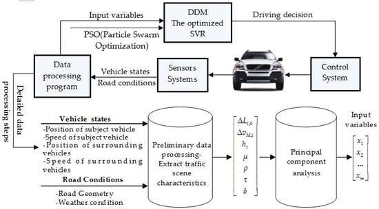
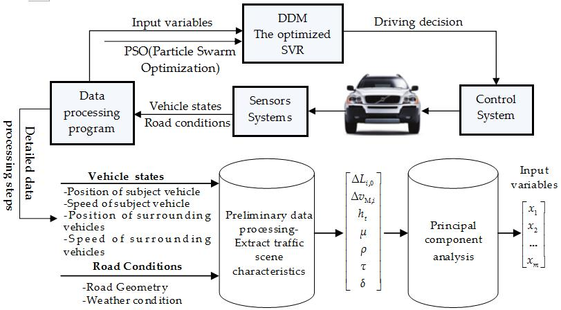
As shown in Figure 1, with the sensor equipment, the autonomous vehicle can sense and collect traffic information, including vehicle states and road conditions in real time, to input them into the designed data processing program for some data processing to obtain the input variables of DDM.
According to these input variables, the DDM searches the relevant information and matches the accurate driving decision with the learning experiences, and then transmits the decision order to the control system. These learning experiences refer to the driving decision-making rules in DDM that are obtained by learning a lot of real driving experience. Then, the control system will control the actuators (include the steering system, pedals, and automatic gearshift) to carry on with the corresponding operation.
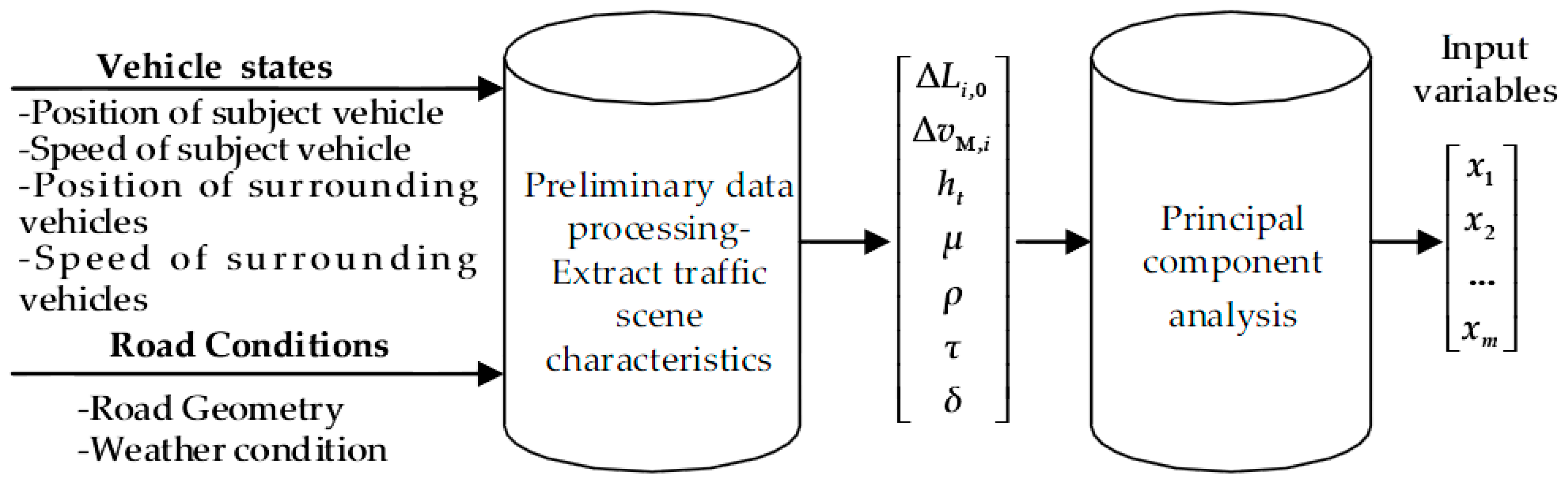
In the whole process of information collection, transmission, and execution, the DDM plays a key role, which is the central system to control the autonomous vehicle. The types of driving decision DDM outputs include free driving, car following, and lane changing. Its input variables are obtained through the preliminary data processing for extracting traffic scenario characteristics as reference indexes and the further data fusion. The method of data fusion adopted in this paper is Principal Component Analysis (PCA). The whole detailed data processing steps in the data processing program are described in Figure 2.
The schematic diagram of vehicle states on a road is shown in Figure 3. All of the above obtained reference indexes in Figure 2 are described as follows:
- /(m): The gap difference between and safe distance , and refers to the distance between the subject vehicle M and vehicle , ;
- /(m/s): The relative speed between vehicle M and vehicle ;
- /(s): The time headway of current lane;
- : Road adhesion coefficient, dimensionless;
- /(m−1): Road curvature;
- : Road slope, percentage; and,
- /(m): Road visibility.
2.1. Support Vector Machine Regression Model
SVR model is a kind of machine learning method based on statistical learning theory, which can improve the generalization ability of learning machine by seeking the minimum structural risk [16,20]. So, SVR model has been widely applied and developed in the fields of pattern recognition, regression analysis, and sequence prediction [18,21].
Let be a set of training samples, each of samples is the input variable, which is obtained from traffic environment features. is the output driving decision corresponding to . These training samples are fitted by , and all of the fitted results must be satisfied with error accuracy , i.e.,:
According to the minimization criteria of structural risk, should make minimum. When considering the exiting fitted errors, the relaxation factors are introduced as , . The best regression result can be derived from the minimum extreme value of the following function:
where is the penalty factor value, .
Then, adopt the dual principle, and set the Lagrange multiplier , to establish the Lagrange equation. Through drafting the parameters , , , and making the drafted formulas equal to 0, the regression coefficient and constant term can be obtained:
After that, the results are substituted into the function to get the regression function:
Finally, the original samples are mapped into a high-dimensional feature space with a kernel function , and calculate the parameters with the same method, as above. The obtained non-linear regression function is:
The common kernels are showed as following:
- Polynomial kernel function:
- Radial basis function:
- Sigmoid kernel function:
Where the dot denotes the inner-product operation in Euclidean space, is the degree of polynomial kernel, is the constant term determining the width of RBF kernel [18]. With different kernels, it can be structured by different regression surfaces, then different training results may be gotten on driving decision-making. So, it is important to select the proper kernel function and kernel parameters in the SVR model.
2.2. The Optimized Support Vector Machine Regression Model
2.2.1. The Selection of Kernel Function
In the research field of SVR model, the selection of kernel function type is the most popular research problem. The kernel function adopted by most of SVR research is the RBF kernel function. But, for different specific problems, the selected kernel function can reflect some of the characteristics of the problem itself [22]. The kernel function specified by researchers based on experience may not be the best choice for specific problems. So, this requires some ways to choose the optimal kernel function for them. In this paper, in order to avoid complexity and one-sidedness of the selection, and to give full play to the benefits that are brought by various kernel functions for the DDM, a weighted hybrid kernel function is proposed:
where , , , respectively, refer to the weight factor and exponential factor corresponding to each kernel function. Then, combine the exponential factor , with and respectively, we can simplify this formula:
The weighting factor needs to be satisfied:
When , it represents that the corresponding kernel function does not play a role in DDM. When , and , then the expression of the formula is similar with the primitive type of Polynomial Kernel.
2.2.2. Parameter Optimization
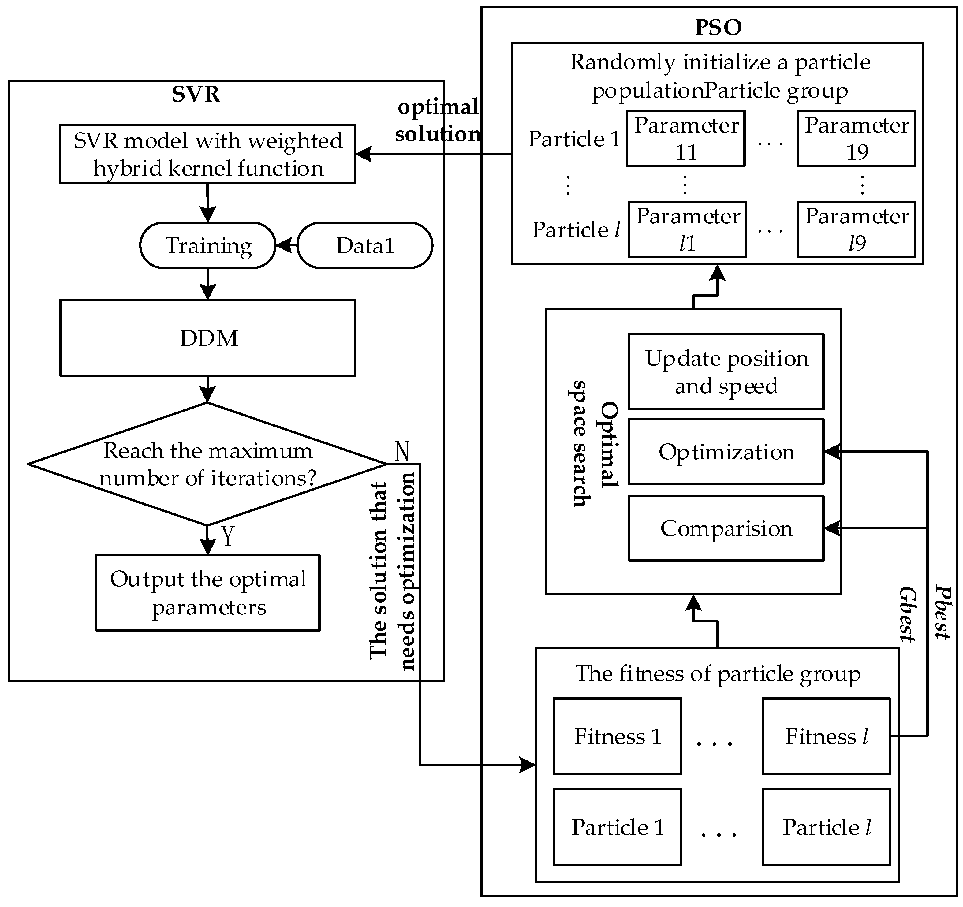
Particle swarm optimization (PSO) algorithm is a new evolutionary and iterative optimization algorithm developed in recent years. PSO algorithm is also started from the random solution and the quality of its solution is evaluated by the fitness. It finds the global optimum following the optimal particles in the solution space [23]. PSO algorithm has a fast convergence rate, and can avoid falling into the local optimum [24,25]. So, in this paper, we adopt PSO algorithm to optimize the undetermined parameters of the SVR model and the weighted hybrid kernel function.
In the PSO algorithm, particles dynamically adjust their positions in the -dimensional space through their individual and peer flight experience. In -dimensional space, the number of particles is , and the position of particle can be represented as , and its flying speed is . The best position visited by the particle so far can be noted as the particle best, i.e., , and the best position found by all the particles so far can be noted as the global best, i.e., . At every moment , the particle will adjust its speed and position by:
where , , is the limited maximum flying speed, and is the uniform random number on the interval , it can increase the searching randomness of particles based on the Pbest and the Gbest.
Then, the PSO-SVR parameter optimization architecture is established in Figure 4. We set the updated step factor as and the positive acceleration coefficients of particle as . The limited maximum flying speed is set to 100, and the number of particles is 50. The number of undetermined parameters is 9, including , in selecting kernel function type, parameters of each single kernel function , , , , , , and SVR penalty factor , it is represented as the dimension of the particle space. The parameter of kernel function and penalty factor are limited in the value range (−10, 10).
The optimization steps are given as follows:
- Step 1
- randomly initialize the positions and speeds of all particles;
- Step 2
- the fitness value of each particle is calculated according to the fitness function of driving decision problem;
- Step 3
- respectively compare the fitness value of each particle with their own and . If the fitness value is larger than , then update with the fitness value. If the fitness value is larger than , then update with the fitness value;
- Step 4
- for each update, reset the SVR penalty factor to create a larger research space for particles, avoid falling into the local area of current optimal value;
- Step 5
- update the position and speed of each particle according to Formulas (8) and (9); and,
- Step 6
- when the number of iterations reaches the maximum set, stop it and output the optimal parameters. Otherwise, return to Step 2.
In this paper, set the training accuracy as the fitness function in the optimized process. In order to evaluate the predicting effect of model for each driving decision, the average absolute error and relative mean square error are selected as the comprehensive evaluation indexes. The former can reflect the degree of deviation between reasoning and measured values, and the latter is the changing embodiment of the error values, which reflects the output stability of SVR model.
3. Experimental Set-Up
A driving experiment needs to be set up to collect relevant data for training the optimized SVR model. Driving simulation is an alternative on-road experiment when the driver desires to use more controllable traffic scenarios to manipulate under certain experimental conditions. By adjusting the light, brightness, motion, audio, etc. in the simulator, it can represent a real traffic scene and an actual vehicle for the driver, which is used to study driving behaviors safely. From the output data, we can obtain the trajectory data of the subject and surrounding vehicles, which are useful to analyze driving decisions.
3.1. Driving Simulator
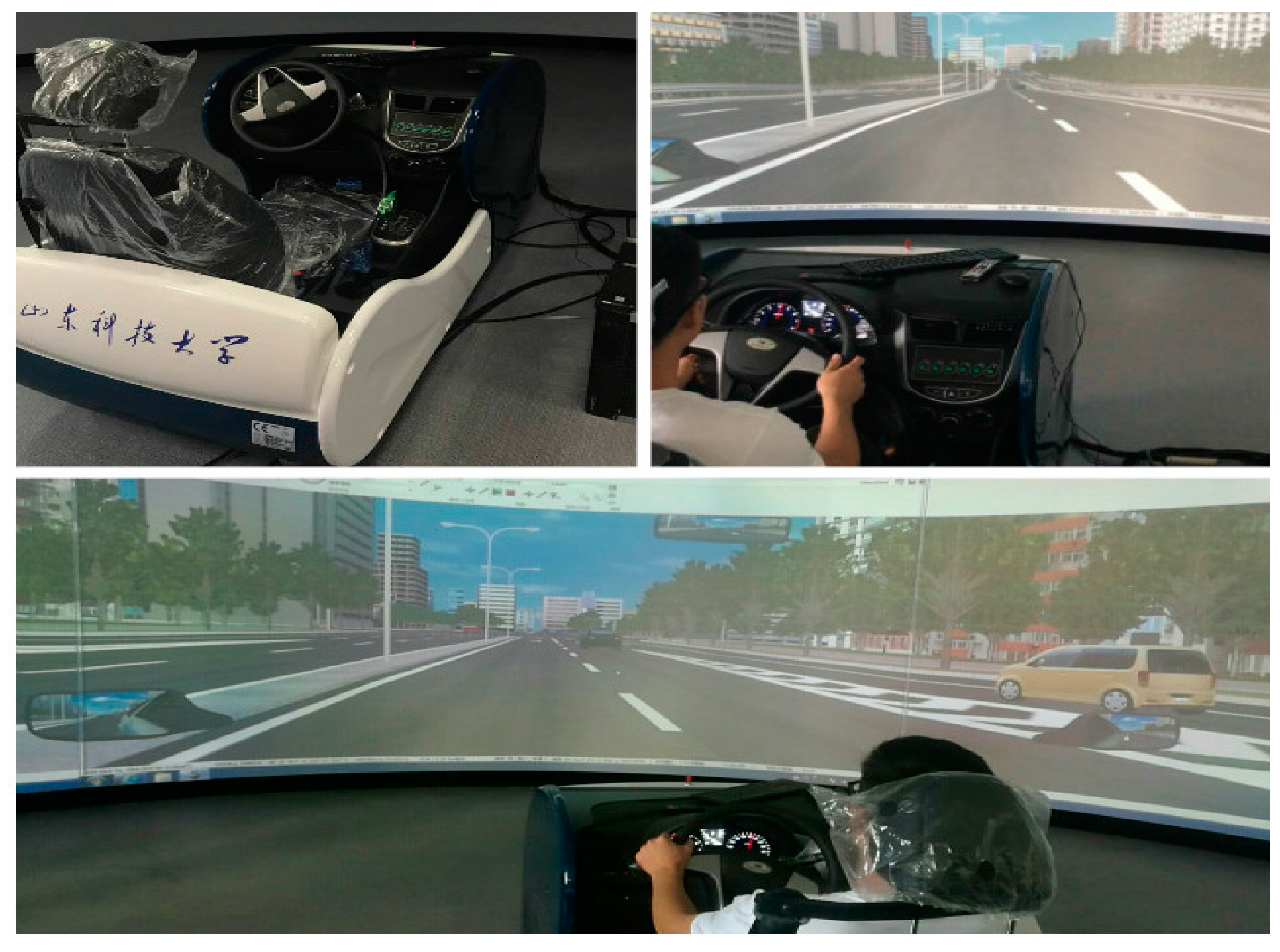
Driving simulation experiment is performed using the UC-win/Road 12.0 driving simulator platform (12.0 version, Fulamba Software Technology Co., Ltd., Shanghai, China, 2016) at the intelligent transportation experimental center of Transportation College in Shandong University of Science and Technology, which is shown in Figure 5. The hardware is made up of three networked computers and some interfaces, such as the steering system, pedals and the automatic gearshift. The traffic environment is projected onto a large visual screen (Fulamba Software Technology Co., Ltd., Shanghai, China) (this big screen is made up of 3 sub-screens), which can provide a 135° field of view. The resolution of visual scene is 1920 × 1080, the refresh rate of the scene is 20–60 Hz depending on the complexity traffic environment. The simulator can record the position coordinates, speed, acceleration of the subject vehicle, and the surrounding vehicle in real time.
3.2. Participants
A total of 31 drivers with different driving experiences are recruited for experiment, including 19 male and 12 female drivers. Before performing driving simulation experiments, a survey for all of the participants is conducted, which is mainly focused on personal driving habits, driving experience, car accident history, physical and psychological status, etc. The average age of the participants is 25.7 years old (std is 3.91 years), ranging from 23 to 37 years. All of the participants have a qualified driver’s license, and more than five years of driving experience (std is 4.33 years). None of participant has any visual and psychological problems. Among 31 participants, three participants (two males, one female) had car crashes in the past five years. The participants are trained to be familiar with the driving simulated operation and to complete the driving simulation on all the traffic environments as required.
3.3. Driving Scenario Setting
A two-way with four-lane urban road section is established for this experiment, as shown in Figure 5. Setting different parameters for vehicles, roads, and traffic, we can establish different traffic simulated scenarios. Set all the vehicles running on these scenarios as standard cars, and the traffic density range to 4–32 veh/km (note: 4–16 veh/km is the low density range, 16–28 veh/km is the middle density range, and 28–32 veh/km is the high density range). The traffic flow is running randomly at each density range with a desired speed of 40–50 km/h. The reference values of the road parameters are shown in Table 1, and the initial set of road parameters are standard values, i.e., (μ, ρ, τ, δ) = (0.75, 0, 0, 1000). The data acquisition frequency is 10 Hz.
3.4. Data Acquisition and Preprocessing
3.4.1. Data Acquisition
The collected data include driving trajectory data of the subject and its surrounding vehicles, their speeds and road environment parameters. According to the following method, the useful driving trajectory data of each driving decision are extracted and classified into the driving decision data set:
- (1)
- Lane changing: The driving trajectory data of 10 s before implementing lane changing are recorded in lane changing data set.
- (2)
- Car following: The driving trajectory data within the 50 m gaps between the subject and its leading vehicle are recorded in car following data set.
- (3)
- Free driving: The driving trajectory data beyond 50 m gaps between the subject and its leading vehicle, and the driving trajectory data output when the subject vehicle with the desired speed are recorded in free driving data set.
After data classification and statistics, a total of 3211 groups of free driving data, 5312 groups of car following data, and 1009 groups of lane changing data are obtained. Each group of driving decision data includes one group of the driving trajectory data, together with their corresponding speeds and the road environment parameters.
3.4.2. Preliminary Data Process
In the preliminary data process, the data contained in all driving decision data sets are calculated to obtain the driving decision samples. From the driving trajectory data, we can obtain , , , and the driving decision (free driving, car following or lane changing), from the speed information, we can obtain , , and , from the road environment parameters, we can obtain the values of μ, ρ, τ, δ. One sample includes one reference index vector and its corresponding driving decision.
3.4.3. The Output and Input Variables of the Optimized SVR Model
(1) The output variables
In this paper, the output variable of the optimized SVR model is a driving decision, may be free driving, car following, or lane changing. We assign the represented values and the output threshold ranges to all of the driving decisions, as seen in Table 2. For example, if an output value of DDM falls within the threshold range (−1.5, 0.5), it represents that the driving decision is free driving.
(2) The input variables
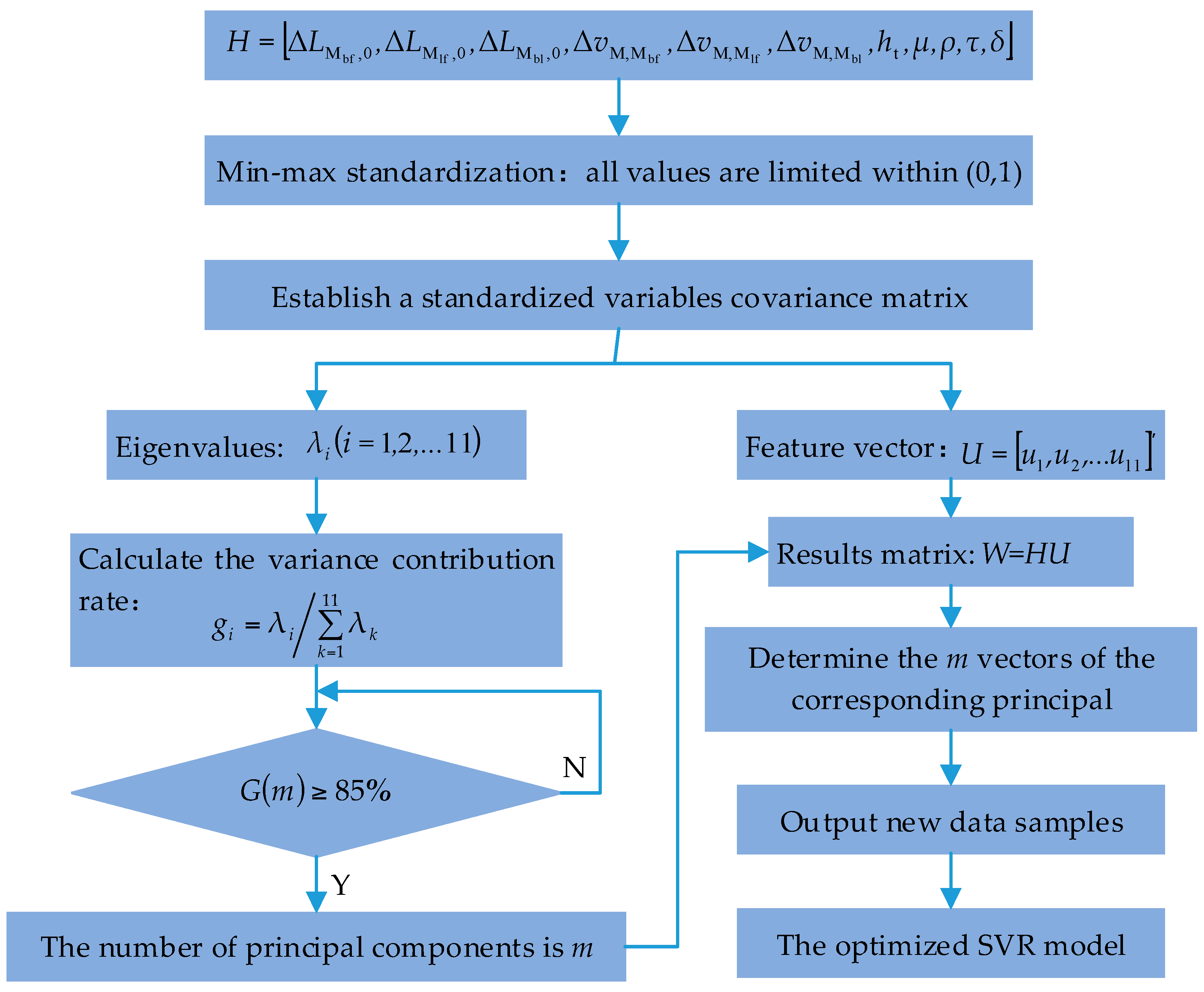
Solving practical problems often need to collect a lot of indexes to reflect more information about the research object. If the correlation between these indexes is high, then the information reflected from them will have a certain overlap, which will increase the complexity of processing information. To solve this problem, Principal Component Analysis (PCA) is proposed to analyze data indexes and obtain the needed input variables [26].
PCA is a statistical analysis method. It can transform multiple correlated indexes into a few of uncorrelated indexes. The comprehensive indexes, called the principal components, will keep the original indexes information as much as possible. If there is a -dimensional random vector , using PCA, the reference indexes can be transformed into a set of uncorrelated principal indexes as their principal components, as seen in (14).
Then, principal components need to be selected from above principal components to adequately reflect the information represented by . The number of principal components depends on the cumulative contribution rate of the variance .
where is the eigenvalue of .
Usually, when , these principal components can adequately reflect the information of the original reference indexes.
Then, we use PCA to make the correlation analysis of 11 reference indexes through 200 sets of samples. The analysis process of PCA is shown in Figure 6. The calculated results of PCA for each principal component are shown in Figure 7. According to the cumulative contribution rate of the variance of each principal component, the first five principal components are selected as the input variables of the optimized SVR model.
4. The Performance of the Optimized SVR Model on Driving Decision-Making
4.1. The Performance of the Weighted Hybrid Kernel Function
In the parameter optimization process of the optimized SVR model, 75% of the driving decision samples are randomly selected for training, and the remaining 25% samples are used for model validation. In order to evaluate the performance of the weighted hybrid kernel function, a SVR model with RBF kernel function is input with the same 75% samples to get its corresponding iteration results. We set to 200 the maximum number of training iterations.
With the PSO algorithm, we can obtain the weighted hybrid kernel function of the optimized SVR model, as shown in formula (16).
The optimal parameters of each basic kernel function incorporated in the weighted hybrid kernel function are shown in the following Table 3. The best penalty factor . In the SVR model with RBF kernel function, the optimal parameters are , . The iterative comparison results of fitted values can be seen from Figure 8.
It can be seen that the fitted accuracy of SVR model with weighted hybrid kernel function and RBF kernel function, respectively, are 92.3% after 31 generations and 89.7% after 43 generations. So, when compared with RBF kernel function, the weighted hybrid kernel function shows better performance on driving decision-making.
4.2. The Performance of SVR Model
BP (Back Propagation) neural network (BPNN) is one of the most widely used and successful learning algorithms in current research, and is particularly suitable for solving complex problems with internal mechanisms [27,28,29]. In order to verify the performance of SVR model, a typical feed-forward BPNN is established to compare with SVR model on the performance of driving decision-making. The BPNN model is established with five layers (an input layer, three hidden layers, and an output layer). Set the Tan-Sigmoid function as the transfer function of BPNN model. The five principal components obtained above are set as its input layer parameters and the corresponding driving decisions is set as the output layer parameter.
In general, the number range of nodes in the hidden layers depends on the number of nodes in the input and output layer [30]. We use our sample data to check the accuracy performance of BPNNs with different number of nodes in the hidden layers, the final number of nodes in each hidden layer is determined to 7. By the parameter adjustment and the test in MATLAB, the number of iterations is determined to 500, the learning rate is 0.01, and the training goal (mean square error) is 1 × 10⁴. Then, the same 75% samples are input into BPNN model for training to obtain the BPNN-based DDM (BPNN-DDM). In the training process, the weights and bias are adjusted continuously to suit the desired output corresponding to the reference indexes. After 48 iterations, the network converges to the desired error. Then, the remaining 25% samples are input into the trained BPNN-DDM and SVR-DDM with RBF kernel function, the reasoning results of SVR-DDM with weighted hybrid kernel function, SVR-DDM with RBF kernel function and BPNN-DDM can be seen in the Table 4.
It can be seen from Table 4 that the SVR-DDM with weighted hybrid kernel function has the best performance in reasoning driving decisions, with the 93.1% accuracy for free driving, 94.7% accuracy for car following, and 89.1% accuracy for lane changing. The reasoning accurate of SVR-DDM with RBF kernel function for three driving decisions is 89.3%, 92.7% and 86.8%, respectively, lower than that of the SVR-DDM with weighted hybrid kernel function, this results are from the optimization of kernel function in SVR Model. When compared with the two SVR-DDMs, the decision reasoning accuracy of BPNN-DDM is lower than SVR-DDM with weighted hybrid kernel function, and has little differences with the SVR-DDM with RBF kernel function. But, the values show that the reasoning stability of the SVR-DDM with RBF kernel function is better than BPNN-DDM. In addition, the three DDMs have the highest accuracy for car following decision, and the lowest accuracy for lane changing. This result may be due to the small number of samples and the complexity of lane changing itself. In summary, the above results support the superior performance of SVR than BPNN in terms of the reasoning accurate, stability, and time, so the SVR model is more suitable for driving decision-making than BPNN model.
4.3. Influence Analysis of Road Conditions on the Reasoning Accuracy of DDM
In order to verify the effects of road conditions on the accuracy of DDM, the reasoning results of three DDMs (include SVR-DDM with weighted hybrid kernel function, SVR-DDM with RBF kernel function and BPNN-DDM) with the following reference index combinations are compared:
- vehicle states + Road conditions are used as inputs; and,
- only vehicle states are used as inputs.
Three DDMs with the first reference index combination has already been trained and validated in the previous Table 4.
For the second reference index combination, road conditions information is eliminated from the above 75% training samples and the remaining 25% testing samples. Then, three DDMs without considering road conditions are established using the same training method and tested with the testing samples. The reasoning results of three DDMs without considering road conditions are shown in the following Table 5.
As illustrated in Table 4 and Table 5, after eliminating the information of road conditions from the reference index set, the accuracy of SVR-DDM with weighted hybrid kernel function for free driving, car following and lane changing is reduced from 93.1% to 82.3%, 94.7% to 85.9% and 89.1% to 78.2%, respectively, SVR-DDM with RBF kernel function is reduced from 89.3% to 78.5%, 92.7% to 82.2% and 86.8% to 76.8% respectively, and the BPNN-DDM is reduced from 89.9% to 78.1%, 91.4% to 80.4% and 87.1% to 75.1% respectively. The results support the effectiveness of making driving decision with road conditions. In addition, although the average reasoning time of DDMs with added road conditions is higher than that of DDMs without added road conditions, the reasoning stability of DDMs with added road conditions is much better than that of DDMs without added road conditions. In general, DDM has better performance on reasoning driving decisions with added road conditions, which is further explained that the road condition cannot be ignored in driving decision-making.
4.4. Sensitive Analysis of Road Conditions on Driving Decisions
It can be seen from the above results that road conditions have a great influence on driving decisions. But how does each parameter affect driving decisions? What is the degree of their effects on each driving decision? A solution is provided to quantitatively evaluate their effects with the SVR-DDM with weighted hybrid kernel function (all of the DDMs mentioned in the following analysis refer to the SVR-DDM with weighted hybrid kernel function and with added road conditions).
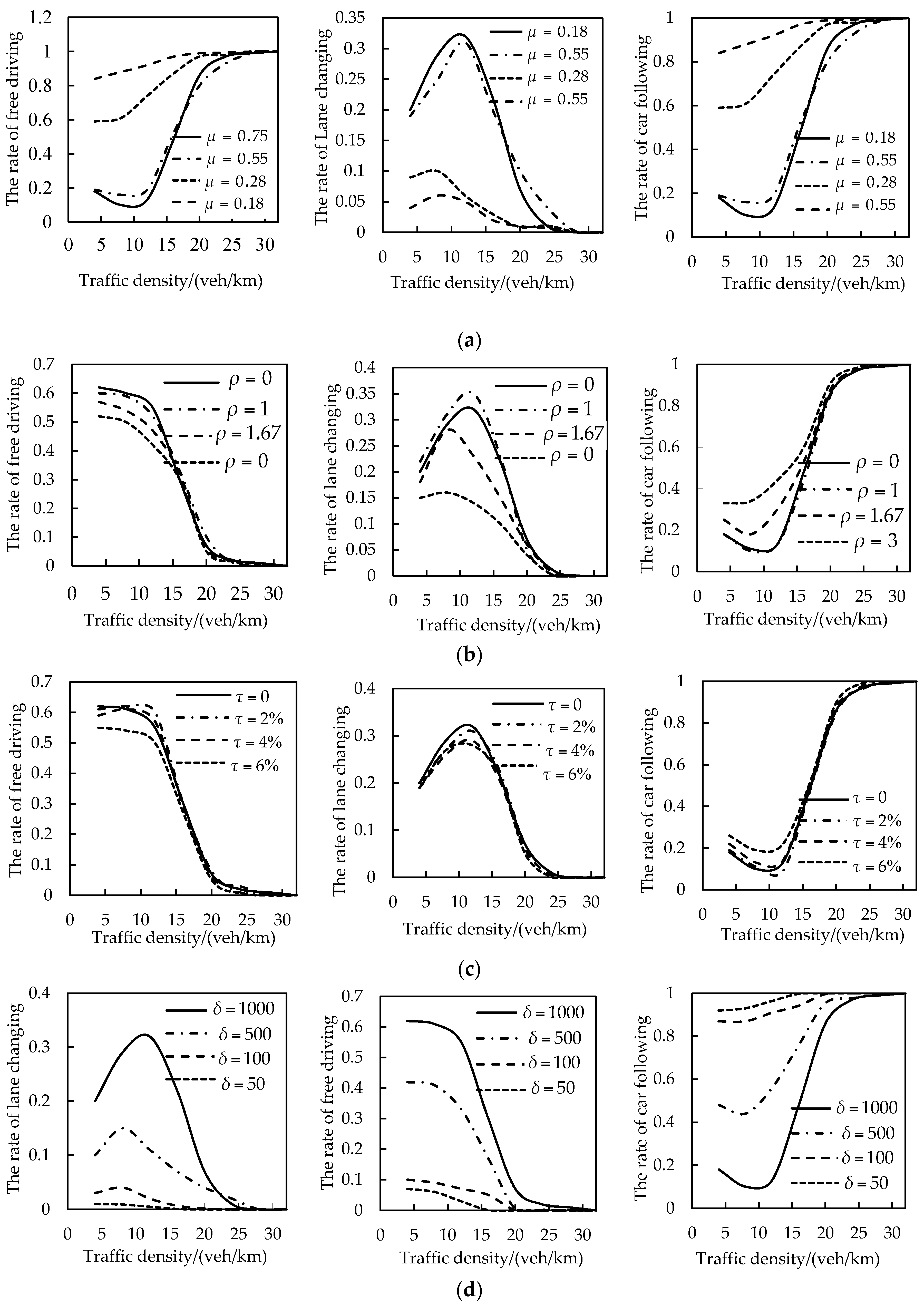
We quantitatively evaluate the effects of each road parameter on driving decisions by analyzing the sensitivity of DDM to the changes in each road parameter. We take the changes in the road adhesion coefficient as an example. Using the driving decision samples under standard road conditions, we first count and calculate the proportions of each driving decision at different traffic density ranges. Then, we make the take values at 0.55, 0.28 and 0.18, respectively. The other three road parameters remain standard. Every time that the changes, a new set of driving decision samples is obtained and input into the DDM. From the output of DDM, the proportion of each driving decision in different traffic density is calculated. Then, we can get the trend that the proportion of each driving decision varies with the traffic density when taken at 0.75, 0.5, 0.25 and 0.18, respectively. In the same way, we can also get the trend that the proportion of each driving decision varies with the traffic density when the other three road parameters take different values, respectively. After this operation and data statistics, the quantitative influence is displayed in Figure 9.
As shown in Figure 9, it can be seen that the changes of road conditions have the greatest influence on the driving decisions in the low traffic density range (4–16 veh/km) and almost have no influence in the high traffic density range (28–32 veh/km). In the low and middle traffic density range (4–28 km/h), road visibility has the greatest effect on driving decision, then followed by adhesion coefficient , road curvature , and road slope . So, we can conclude: in the low traffic density range, driving decision-making is mainly restricted by the road conditions, in consequence, results are easy to be wrong without considering road conditions. on the other hand, with the high traffic density range, driving decision-making is mainly limited by vehicles states, so even if road conditions are not taken into account, the reasoning results are less affected.
Take the change rate of driving decision in low traffic density range in Figure 9b as an example, when all of the road parameters are taken as the standard values, the average rates of free driving, lane changing, and car following are about 0.469, 0.262, and 0.269, respectively, in the low traffic density range. If is changed to 100, the average rates of three driving decisions are changed to about 0.078, 0.034, 0.888, respectively, which means that about 61.9% of samples change their decisions when the road visibility is changed from 1000 m to 100 m. Similarly, if is changed to 4%, then the average rates of three driving decisions are changed to 0.515, 0.238, and 0.247, respectively, which means that about 4.6% of samples change their decisions when the road slope is changed from 0 to 4%. The same is true for the analysis of driving decisions corresponding to the changes in other two parameters. Thus, it can be seen that road conditions are important indexes that cannot be ignored in DDM for autonomous vehicle.
5. Conclusions
In this paper, a SVR model was developed to make accurate driving decisions for autonomous vehicle. Our model was optimized by a weighted hybrid kernel function and a PSO algorithm. Road conditions and vehicle states were simultaneously as the reference indexes of DDM. The driving decisions that were made by DDM included free driving, car following, and lane changing. Then, driving simulated experiments with different traffic environments were executed to extract the driving decision samples. The optimized SVR model was trained and validated with the training and testing samples to establish DDM. Our model was compared with: (1) a SVR model with RBF kernel function, and (2) BPNN model. The comparison results showed that the accuracy of our optimized SVR model was the best, with more than 92% accuracy. Besides, the results also showed that our optimized SVR model had a better performance in free driving and car following with 93.1% and 94.7% of accuracy, respectively, than lane changing decision with 89.1% of accuracy.
Finally, we investigated the effect of road conditions on the accuracy of DDM and quantified their effects on each driving decision through the sensitive analysis. The results showed that road conditions almost had almost no influence on driving decisions with high traffic density range, and had the greatest influence with low traffic density range. In the low and middle traffic density, road visibility has the greatest effect on the driving decisions, then followed by , , and . To some extent, the verified results were consistent with the actual driving experience, which indicated the reasonability of the obtained DDM with added road conditions.
Even though the DDM based on the optimized SVR model is able to reason driving decisions, and outperforms other models that are proposed in this paper, there are still some weak points and limits, such as the sample size of lane changing decision is smaller than that of car following and free driving, and that the DDM has not yet been implemented in real road environment, we will improve them in the future. In addition, future research will focus on establishing a DDM used in dangerous driving environments, for example, if a pedestrian or vehicle suddenly present in front of the subject vehicle, then the subject vehicle should make proper driving decision, like steering, braking, or steering and braking.
Acknowledgments
This work was financially supported by the Natural Science Foundation of China under Grant no. 51678320, the Outstanding Young Scientists Research Award Foundation of Shandong Province under Grant no. ZR2016EEB06, the Scientific Research Foundation of Shandong University of Science and Technology for Recruited Talents under Grant no. 2015RCJJ035.
Author Contributions
The corresponding authors Junyou Zhang and Yaping Liao proposed this research and designed the experiments; The corresponding authors Shufeng Wang and Jian Han performed the experiments and analyzed the experimental data; Junyou Zhang was responsible to the analysis of model and drafted the manuscript with the help of Yaping Liao. Shufeng Wang and Jian Han proposed some amendment opinions and helped to improve this paper.
Conflicts of Interest
The authors declare no conflict of interest.
References
- Lv, W.; Song, W.G.; Liu, X.D.; Ma, J. A Microscopic Lane Changing Process Model for Multilane Traffic. Phys. A Stat. Mech. Appl. 2013, 392, 1142–1152. [Google Scholar] [CrossRef]
- Julia, N.; Brannstrom, M.; Coelingh, E.; Fredriksson, J. Lane Change Maneuvers for Automated Vehicles. Trans. Intell. Transp. Syst. 2017, 18, 1087–1096. [Google Scholar]
- Zheng, J.; Suzuki, K.; Fujita, M. Car-following Behavior with Instantaneous Driver–vehicle Reaction Delay: A Neural-network-based Methodology. Transp. Res. Part C Emerg. Technol. 2013, 36, 339–351. [Google Scholar] [CrossRef]
- Feng, S.M.; Li, J.Y.; Ding, N.; Nie, C. Traffic Paradox on A Road Segment Based on A Cellular Automaton: Impact of Lane-changing Behavior. Phys. A Stat. Mech. Appl. 2015, 428, 90–102. [Google Scholar] [CrossRef]
- Suh, J.S.; Kim, B.J.; Yi, K.S. Design and Evaluation of a Driving Mode Decision Algorithm for Automated Driving Vehicle on a Motorway. IFAC-PapersOnLine 2016, 49, 115–120. [Google Scholar] [CrossRef]
- Wang, X.Y.; Yang, X.Y. Research on Decision Making Mechanism of Driving Behavior Based on Decision Tree. J. Syst. Simul. 2008, 20, 415–419, 448. [Google Scholar]
- Zheng, J.; Suzuki, K.; Fujita, M. Predicting driver’s lane-changing decisions using a neural network model. Simul. Model. Pract. Theory 2014, 42, 73–83. [Google Scholar] [CrossRef]
- Noh, S.; An, K. Decision-Making Framework for Automated Driving in Highway Environments. IEEE Trans. Intell. Transp. Syst. 2017, 1–14. [Google Scholar] [CrossRef]
- Geng, X.L.; Liang, H.W.; Xu, H.; Yu, B. Influences of Leading-Vehicle Types and Environmental Conditions on Car-Following Behavior. Int. Fed. Autom. Control 2016, 49, 151–156. [Google Scholar] [CrossRef]
- Hamdar, S.H.; Qin, L.Q.; Talebpour, A. Weather And Road Geometry Impact on Longitudinal Driving Behavior: Exploratory Analysis Using An Empirically Supported Acceleration Modeling Framework. Transp. Res. Part C 2016, 67, 193–213. [Google Scholar] [CrossRef]
- Hoogendoorn, R.G.; Hoogendoorn, S.P.; Brookhuis, K.A.; Daamen, W. Simple and multi-anticipative car-following models: Performance and parameter value effects in case of fog. In Proceedings of the Transportation Research Board (TRB) Traffic Flow Theory and Characteristics Committee (AHB45) Summer Meeting, Annecy, France, 27 June 2010; pp. 2–16. [Google Scholar]
- McLean, J. Driver speed behavior and rural road alignment design. Traffic Eng. Control 1981, 22, 208–211. [Google Scholar]
- Broughton, K.L.M.; Switzer, F.; Scott, D. Car Following Decisions under Three Visibility Conditions and Two Speeds Tested with a Driving Simulator. Accid. Anal. Prev. 2007, 39, 106–116. [Google Scholar] [CrossRef] [PubMed]
- Wang, H.; Ma, S.-H. Car-following Model and Simulation with Curves and Slopes. Civ. Eng. 2005, 38, 106–111. [Google Scholar]
- Olofsson, B.; Lundahl, K.; Berntorp, K.; Nielsen, L. An Investigation of Optimal Vehicle Maneuvers for Different Road Conditions. IFAC Proc. Vol. 2013, 46, 66–71. [Google Scholar] [CrossRef]
- Shafizadeh-Moghadam, H.; Tayyebi, A.; Ahmadlou, M.; Delavar, M.R.; Hasanlou, M. Integration of genetic algorithm and multiple kernel support vector regression for modeling urban growth. Comput. Environ. Urban Syst. 2017, 65, 28–40. [Google Scholar] [CrossRef]
- Wei, D.L.; Liu, H.C. Analysis of asymmetric driving behavior using a self-learning approach. Transp. Res. Part B Methodol. 2013, 47, 1–14. [Google Scholar] [CrossRef]
- Qiu, X.P.; Liu, Y.L. A car-following model based on support vector machine. J. Chongqing Jiaotong Univ. (Nat. Sci. Ed.) 2015, 34, 128–132. [Google Scholar]
- Yu, R.J.; Abdel-Aty, M. Utilizing support vector machine in real-time crash risk evaluation. Accid. Anal. Prev. 2013, 55, 252–259. [Google Scholar] [CrossRef] [PubMed]
- Hong, W.-C.; Dong, Y.C.; Zheng, F.F.; Lai, C.-Y. Forecasting urban traffic flow by SVR with continuous ACO. Appl. Math. Model. 2011, 35, 1282–1291. [Google Scholar] [CrossRef]
- Zhu, L.L.; Liu, L.; Zhao, X.P.; Yang, D. Study on Vehicle Driving Behavior Recognition Based on Support Vector Machine. J. Transp. Syst. Eng. Inf. 2017, 17, 91–97. [Google Scholar]
- Yang, D.G.; He, C.W.; Li, M.; He, Q.G. Behavioral Recognition of Vehicle Steering and Lane Based on Support Vector Machine. J. Tsinghua Univ. (Sci. Technol.) 2015, 55, 1093–1097. [Google Scholar]
- Gold, C.; Sollich, P. Model selection for support vector machine classification. Neurocomputing 2003, 55, 221–249. [Google Scholar] [CrossRef]
- Rokonuzzaman, M.; Sakai, T. Calibration of the parameters for a hardening-softening constitutive model using genetic algorithms. Comput. Geotech. 2010, 37, 573–579. [Google Scholar] [CrossRef]
- Babazadeh, A.; Poorzahedy, H.; Nikoosokhan, S. Application of particle swarm optimization to transportation network design problem. J. King Saud Univ. Sci. 2011, 23, 293–300. [Google Scholar] [CrossRef]
- Deng, W.; Zhao, H.M.; Yang, X.H.; Xiong, J.X.; Meng, S.; Bo, L. Study on an improved adaptive PSO algorithm for solving muli-objective gate assignment. Appl. Soft Comput. 2017, 59, 288–302. [Google Scholar] [CrossRef]
- Saha, P.; Roy, N.; Mukherjee, D.; Sarkar, A.K. Application of Principal Component Analysis for Outlier Detection in Heterogeneous Traffic Data. Procedia Comput. Sci. 2016, 83, 107–114. [Google Scholar] [CrossRef]
- Chen, Y.; Yi, Z.-C. The BP artificial neural network model on expressway construction phase risk. Syst. Eng. Procedia 2012, 4, 409–415. [Google Scholar] [CrossRef]
- Tang, J.J.; Liu, F.; Zhang, W.H.; Ke, R.M.; Zou, Y.J. Lane-changes prediction based on adaptive fuzzy neural network. Expert Syst. Appl. 2018, 91, 452–463. [Google Scholar] [CrossRef]
- Peng, J.S.; Guo, Y.S.; Fu, R.; Yuan, W.; Wang, C. Multi-parameter prediction of drivers’ lane-changing behaviour with neural network model. Appl. Ergon. 2015, 50, 207–217. [Google Scholar] [CrossRef] [PubMed]
Figure 1.
Schematic architecture of the driving decision-making process of autonomous vehicle. DDM: Driving Decision-making Mechanism.
Figure 1.
Schematic architecture of the driving decision-making process of autonomous vehicle. DDM: Driving Decision-making Mechanism.

Figure 2.
The detailed data processing of data processing program.

Figure 3.
Diagrammatic sketch of vehicle states.
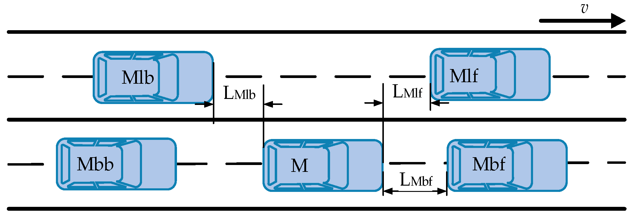
Figure 4.
The steps of Particle Swarm Optimization (PSO)—Support Vector Machine Regression (SVR) parameters optimization architecture.
Figure 4.
The steps of Particle Swarm Optimization (PSO)—Support Vector Machine Regression (SVR) parameters optimization architecture.

Figure 5.
Traffic Simulation Scene of Simulated Driving Test.

Figure 6.
The analysis process of driving decision samples using Principal Component Analysis (PCA).
Figure 6.
The analysis process of driving decision samples using Principal Component Analysis (PCA).

Figure 7.
The results of principal component analysis for 11 reference indexes.
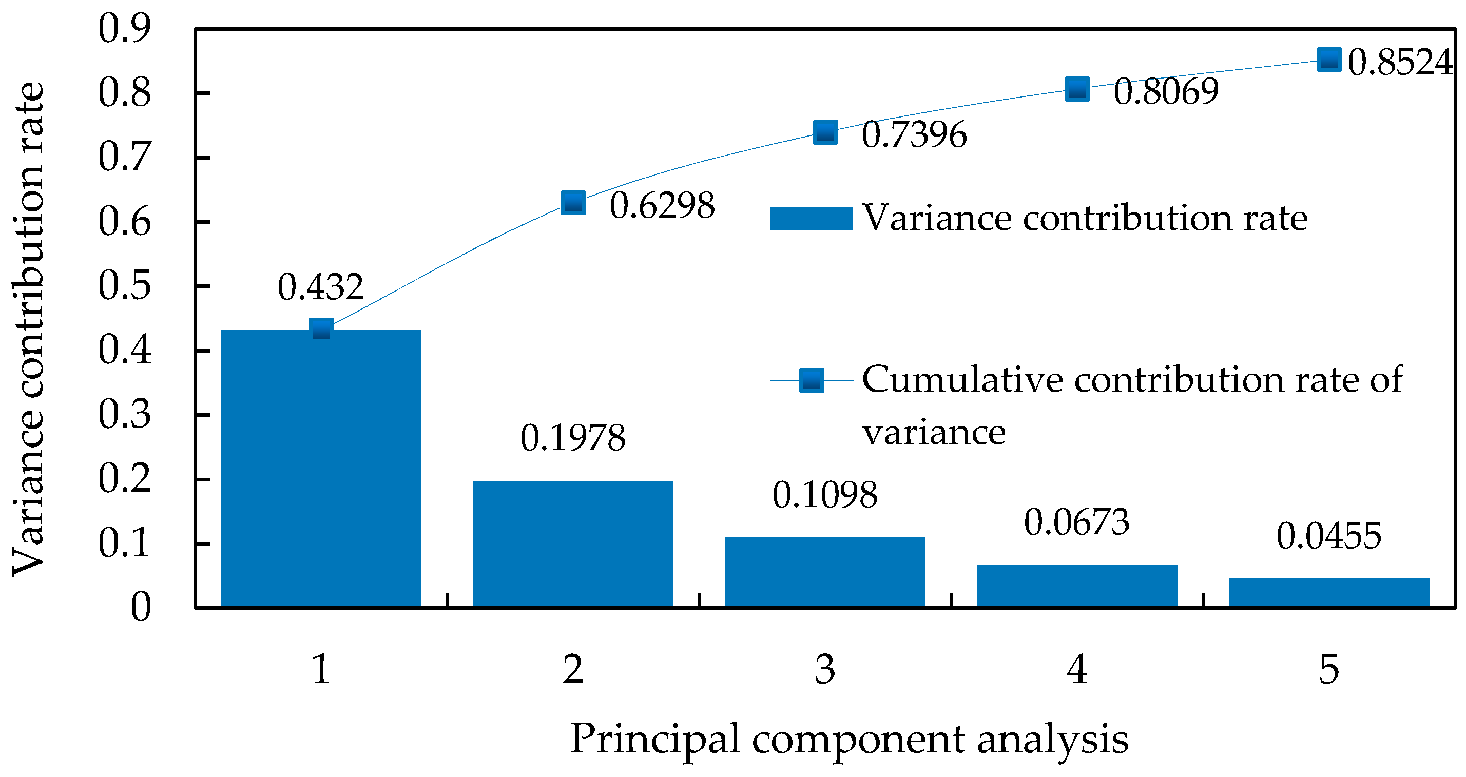
Figure 8.
The iterative comparison results of fitted values of two SVR models.
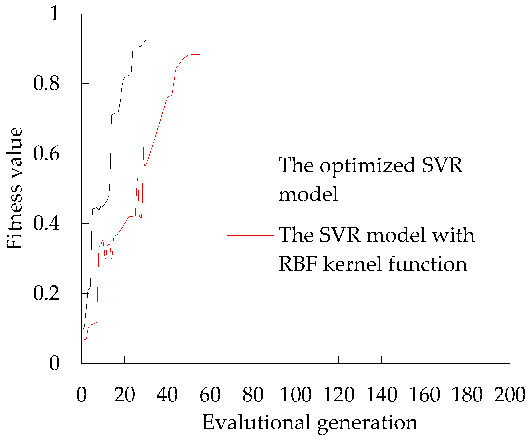
Figure 9.
Driving Decision Rate under Different Road Conditions. (The horizontal axis in these diagrams represents the traffic flow density, and the vertical axis represents the rate of each driving decision (between 0 and 1). The solid lines in all diagrams represent the changing trend of the proportion of driving decisions with traffic density under standard road conditions. (a) The changing trend of each driving decision rate with traffic density when takes different values; (b) The changing trend of each driving decision rate with traffic density when takes different values; (c) The changing trend of each driving decision rate with traffic density when takes different values; (d) The changing trend of each driving decision rate with traffic density when takes different values. From left to right, each column represents the trend of lane changing rate, free driving rate and car-following rate with traffic density when each road parameter is taken as different values, respectively.).


Table 1.
Settings of Road Parameters.
| Road Parameters | Setting Values |
|---|---|
| Adhesion coefficient | 0.75/0.55/0.28/0.18 |
| Road curvature (m−1) | 0/3/1.67/1 |
| Road slope | 0/2%/4%/6% |
| Road visibility /m | 1000/500/100/50 |
Table 2.
Driving Decision-Making Behaviors.
| Driving Decision | Symbol | Represented Value | Threshold Range of the Output Value |
|---|---|---|---|
| Free driving | −1 | (−1.5, 0.5) | |
| Car following | 0 | (−0.5, 0.5) | |
| Lane Changing | 1 | (0.5, 1.5) |
Table 3.
The best parameters of each basic kernel function.
| The Basic Kernel Function | Optimal Parameters | |||||
|---|---|---|---|---|---|---|
| Polynomial kernel function | 12.114 | 3.741 | 0.097 | - | - | - |
| Radial basis function | - | - | - | 60.565 | - | - |
| Sigmoid kernel function | - | - | - | - | 13.255 | 1.651 |
Table 4.
The reasoning results of three driving decision-making mechanism (DDMs). SVR: Support Vector Machine Regression; RBF: Radial Basis Function; BPNN: Back Propagation neural network.
Table 4.
The reasoning results of three driving decision-making mechanism (DDMs). SVR: Support Vector Machine Regression; RBF: Radial Basis Function; BPNN: Back Propagation neural network.
| Type | Driving Decision | Reasoning Accuracy Rate | Average Reasoning Time | ||
|---|---|---|---|---|---|
| SVR-DDM with weighted hybrid kernel function | Free driving | 93.1% | 0.090 | 0.347 | 0.004 s |
| Car following | 94.7% | 0.057 | 0.121 | ||
| Lane changing | 89.1% | 0.101 | 0.723 | ||
| SVR-DDM with RBF kernel function | Free driving | 89.3% | 0.127 | 0.655 | 0.003 s |
| Car following | 92.7% | 0.091 | 0.319 | ||
| Lane changing | 86.8% | 0.142 | 0.981 | ||
| BPNN-DDM | Free driving | 89.9% | 0.121 | 0.844 | 0.009 s |
| Car following | 91.4% | 0.091 | 0.327 | ||
| Lane changing | 87.1% | 0.138 | 1.362 |
Table 5.
The results of three DDMs without considering road conditions.
| Type | Driving Decision | Reasoning Accuracy Rate | Average Reasoning Time | ||
|---|---|---|---|---|---|
| SVR-DDM with weighted hybrid kernel function | Free driving | 82.3% | 0.145 | 1.566 | 0.003 s |
| Car following | 85.9% | 0.138 | 1.441 | ||
| Lane changing | 78.2% | 0.158 | 1.845 | ||
| SVR-DDM with RBF kernel function | Free driving | 78.5% | 0.157 | 1.634 | 0.002 s |
| Car following | 82.2% | 0.155 | 1.521 | ||
| Lane changing | 76.8% | 0.173 | 1.848 | ||
| BPNN-DDM | Free driving | 78.1% | 0.171 | 1.859 | 0.006 s |
| Car following | 80.4% | 0.159 | 1.723 | ||
| Lane changing | 75.1% | 0.176 | 1.877 |
© 2017 by the authors. Licensee MDPI, Basel, Switzerland. This article is an open access article distributed under the terms and conditions of the Creative Commons Attribution (CC BY) license (http://creativecommons.org/licenses/by/4.0/).
Share and Cite
MDPI and ACS Style
Zhang, J.; Liao, Y.; Wang, S.; Han, J. Study on Driving Decision-Making Mechanism of Autonomous Vehicle Based on an Optimized Support Vector Machine Regression. Appl. Sci. 2018, 8, 13. https://doi.org/10.3390/app8010013
AMA Style
Zhang J, Liao Y, Wang S, Han J. Study on Driving Decision-Making Mechanism of Autonomous Vehicle Based on an Optimized Support Vector Machine Regression. Applied Sciences. 2018; 8(1):13. https://doi.org/10.3390/app8010013
Chicago/Turabian StyleZhang, Junyou, Yaping Liao, Shufeng Wang, and Jian Han. 2018. "Study on Driving Decision-Making Mechanism of Autonomous Vehicle Based on an Optimized Support Vector Machine Regression" Applied Sciences 8, no. 1: 13. https://doi.org/10.3390/app8010013
Note that from the first issue of 2016, this journal uses article numbers instead of page numbers. See further details here.