Pareto Optimal Solutions for Network Defense Strategy Selection Simulator in Multi-Objective Reinforcement Learning

Abstract

Using Pareto optimization in Multi-Objective Reinforcement Learning (MORL) leads to better learning results for network defense games. This is particularly useful for network security agents, who must often balance several goals when choosing what action to take in defense of a network. If the defender knows his preferred reward distribution, the advantages of Pareto optimization can be retained by using a scalarization algorithm prior to the implementation of the MORL. In this paper, we simulate a network defense scenario by creating a multi-objective zero-sum game and using Pareto optimization and MORL to determine optimal solutions and compare those solutions to different scalarization approaches. We build a Pareto Defense Strategy Selection Simulator (PDSSS) system for assisting network administrators on decision-making, specifically, on defense strategy selection, and the experiment results show that the Satisficing Trade-Off Method (STOM) scalarization approach performs better than linear scalarization or GUESS method. The results of this paper can aid network security agents attempting to find an optimal defense policy for network security games.

1. Introduction

Computer network security plays a vital role in many organizations today. Business services heavily depend on the reliability of the network. Especially, for companies who provide 24/7 services across the globe, network security plays a core role in the business. The Internet acts as a backbone to these networks. The open architectural nature of the Internet opens inevitable security vulnerabilities to the connected networks and devices.

Over the last few decades, researchers have focused on automating the process of network security management [1]. One of the main problems with the current research approach is addressing network security based on heuristics. To address this issue, recently, there has been a growing body of research focused on systematic analysis of network security using game theory. Game theory provides a systematic method to analyze and predict complex attack-defense scenarios.

It is important for security researchers to keep pace with the rapidly evolving threats and the continuous development of networking technology. The technological advances both complement, as well as hinder, network security since they act as new tools for wrongdoers. Network security involves securing more than one aspect to the network, such as confidentiality, integrity, and availability. Multi-objective optimization in network security have been widely employed to reflect this need. And can be applied to threatening similar security problems arise such as of Internet of Things [2,3,4,5]. Especially, in the case that the mobile nodes, e.g., normal nodes and not the malicious ones, form coalitions in order to achieve a common goal. It is of great interest to research the damage imposed by the attacker and how the proposed framework can provide solution in such types of problems. Multi-objective optimization has attracted many mathematicians and several approaches have been proposed to increase the efficiency and accuracy of the optimal solutions. There is an emerging growth of research interest in the study that uses multi-objective optimization on stochastic game theoretic models. One of the key problems in multi-objective optimization is choosing optimal solutions from a set of solutions. Among other approaches, the most natural and popular method among researchers is scalarization of an objective vector [6].

In this paper, we compare three different types of scalarization approaches with Reinforcement Learning in the context of strategic defense action selection for a defender during interactive attack scenarios. We assume that the defender does not know what move the attacker will make, but must instead respond to previous attack moves.

In recent years, Reinforcement Learning (RL) has received growing attention in the research community. Our work is an extension of our previous work on network defense strategy selection with Reinforcement Learning and Pareto Optimization [7], in which we combined Pareto optimization with Q-learning to find an optimal solution.

The usage of Reinforcement Learning allows for the creation of an offline system that improves over time. The algorithm retains the contribution of every attack-defense interaction and will eventually outperform algorithms that start every new interaction from scratch.

The Pareto-Q-learning approach presents several problems, which we aim to resolve with this study. First is how to choose a solution from the remaining Pareto optimal fronts. As previously indicated, many researchers use scalarization of an objective vector. We examine the efficiency and effectiveness of several scalarization methods. The second problem is the efficiency of the Pareto-Q-learning approach. Previous researches show that direct application and calculation of Pareto fronts for every step in the Q-learning process is onerous and inefficient. Our research explores if the usage of a scalarization algorithm can provide us with a more efficient solution. Finally, our previous game model lacked real-world application. We have updated the model to represent an abstracted DDOS attack.

Single-objective optimization often fails to reflect the variety of complex real-world scenarios [8]. Most of the problems in real life involving decision-making depends on multiple objectives [9,10]. Multi-objective decision-making has been a widely explored area [11]. Multi-objective problems are also known as multi-criteria optimization, or vector minimization [12]. Traditional methods, such as linear programing and gradient descent, are too complex for solving multi-objective Pareto-optimal fronts [13,14]. Multi-Objective Reinforcement Learning has been actively researched in various fields [11]. In traditional reinforcement learning an agent learns and takes action based on receiving a scalar reward from the dynamic environment. The quality of estimate improves over time as the agent tries to maximize the cumulative reward [15]. Sutton’s [15] reward hypothesis states that goals and purposes can be thought of as maximization of the cumulative single scalar reward. Thus, a single scalarized reward is adequate to represent multiple objectives [11]. Since traditional RL focuses on a single objective, the algorithm requires a modification to accommodate multi-objective problems. The most common approach to deal with multi-objective problems is scalarization.

Scalarization of multi-objective RL involves two steps. First, we specify the scalarization function $f$, such that the $V^{\pi }$ state value vector is projected into a scalar value $V_{\mathit{w}}^{\pi }\left(x\right)=f\left(V^{\pi }\left(x\right),\mathit{w}\right)$, where $\mathit{w}$ is the weight vector parametrizing $f$. Then, we define an objective function with an additive scalar return, such that for all policies $\pi$ and states $x$, the expected return equals the scalarized value of $V_{\mathit{w}}^{\pi }\left(x\right)$. The simplest and most popular, as well as, historically, the first proposed scalarization technique, is linear scalarization [16]. In linear scalarization, $\mathit{w}$ represents the relative weight of the objectives. Since it is a convex combination of all objectives, linear scalarization lacks the ability to find all solutions in a non-convex Pareto set [17]. Lizotte et al. [12] proposed an offline algorithm that uses linear function approximation. Although the method reduces the asymptotic space and complexity of the bootstrapping rule, generalizing the concept into higher dimensions is not straightforward. Commonly known non-linear scalarization, among others, includes the Hiriart-Urruty function [18] and Gerstewitz functions [19].

Another class of algorithm for solving multi-objective problems are evolutionary algorithms (EA). Multi-objective EA (MOEA) uses an evolving population of solutions to solve the Pareto fronts in a single run. Deb and Srinavas [20] proposed non-dominated sorting in a genetic algorithm (NSGA) to solve multi-objective problems. Despite NSGA being able to capture several solutions simultaneously, it has several shortcomings, such as high computation complexity, lack of elitism, and specification of sharing parameters. NSGA-II improves by addressing these issues [21]. Other EA algorithms includes Pareto-archived evolution strategy (PAES) [20] and strength Pareto EA (SPEA). For a thorough survey of multi-objective evolutionary algorithms, the interested reader is referred to [22].

In [23], Miettinen and Mäkelä studied two categories of scalarization functions: classification and reference point-based scalarization functions. In classification, the current solution is compared to the desired value, whereas in reference point-based scalarization functions a reference point is used to represent the aspiration level of the decision-maker (DM) and can be specified irrespective of the current solution.

Benayoun et al. [24] used a step method (STEM) in which the DM classifies the current solution points into two classes, $I^{<}$ and $I^{\ge }$. The DM defines the ideal upper bounds for each objective function. This method requires global ideal and nadir points. Non-differentiable Interactive Multi-Objective Bundle-based optimization System (NIMBUS) is another method that asks the DM to classify objective functions [25]. Additionally, this method requires a corresponding aspirational level and upper bounds.

Since MORL has different optimal policies with respect to different objectives, different optimal criteria can be used. Some of these include lexicographical ordering [26] and linear preference ordering [27]. However, the most common optimal criterion is Pareto optimality [28].

In this paper, we compare the performance of our implementation of Pareto-Q-learning with different reference point-based scalarization methods. We limited our study to three well-known methods: linear scalarization, the satisficing trade-off method (STOM), and the Guess method.

The rest of the paper is organized as follows: In the next section, the related works and background of the different scalarization techniques are covered. In Section 3, we detail the theory and experimental design. Before the conclusion, the experimental results are analyzed in Section 4. Section 5 concluded in this paper.

2. Theory

2.1. Multi-Objective Optimization

In our previous work on multi-objective optimization [7], we discuss the concepts of multi-objective optimization, reinforcement learning, and Pareto optimization in great detail. In this paper, we describe a maximization multi-objective problem with Equations (1) and (2):

$$maxF\left(x\right)=max\left\{f^m\left(x\right)\right\},m\in M$$

(1)

under the condition:

$$x\in X$$

(2)

where $m=\left\{1,2,\dots ,i\right\}$ is the number of objectives, $x={\{x_1,x_2,\dots ,x_n)}^T$ is the vector of variables, and $f^i$ is the value of $i$-th objective. The problem is to simultaneously maximize all the values of objective vector F.

2.2. Pareto Optimization

The solution $x\in X$ is said to be Pareto optimal if there does not exist another $x^{*}\in X$:

$$f^m\left(x^{*}\right)\le f^m\left(x\right),m\in M$$

(3)

and:

$$f^m\left(x^{*}\right)<f^m\left(x\right)$$

(4)

for at least one index $m\in M$.

Pareto set dominance describes a situation where, for a set X and a set Y, X is said to dominate Y, if and only if X contains a vector x that dominates all vectors in set Y, as shown in Equation (5):

$$X\preccurlyeq Y≔\exists \mathit{x}\in X,\forall y\in Y:\mathit{x}\preccurlyeq y$$

(5)

2.3. Reinforcement Learning

RL is a Markov decision process (MDP) in which the agent interacts with an environment to maximize a long-term return from the states [29]. At time step $t$, the agent receives a state $s\in S$, and selects action $a\in A$, following a policy $\pi$, where $\pi$ is a mapping from state $s_t$ to action $a_t$. Transitioning from the current state, $s_t$, to the next state, $s_{t+1}$, has an associated transition probability $P\left(s_{t+1}\right|s_t,a_t)$, for taking the action $a_t$ and an immediate reward $r_t=R_{a_t}\left(\pi \left(s_t\right)\right)$. In order to favor the immediate reward over future rewards, the expected cumulative reward ${\sum }_k^{\infty }\gamma {}^k{r}_{t+k}$ is discounted with a discount factor $\gamma \in \left[0,1\right]$. The goal is to maximize the cumulative long-term reward.

The state value $V^{\pi }$ is the expected return for following policy $\pi$ from state $\mathrm{s}$ defined as in Equation (6):

$$V^{\pi }\left(s\right)=E\{{{\displaystyle \sum }}_k^{\infty }\gamma {}^k{r}_{t+k+1}|\pi ,s_t=s\}$$

(6)

As depicted in Equation (7), the $Q$-value $Q\left(s,a\right)$ stores the action value for taking action $\mathrm{a}$ in state $\mathrm{s}$ and then following policy $\pi$. The $Q$-value is updated iteratively:

$$Q^{\pi }\left(s,a\right)=V^{\pi }\left(s\right)=R_s\left(\pi \left(a\right)\right)+\gamma {\mathrm{\Sigma }}_{s^{*}}{P}_{s,s^{*}}\left(\pi \left(s\right)\right)V^{\pi }\left(s^{*}\right)$$

(7)

The optimal $Q$-value $Q^{{\pi }^{*}}$ determines the best action for a given state by following the optimal policy ${\pi }^{*}$ that gives maximum returns. This is achieved by the recursive Bellman optimality equation [30], which is define bellow in Equation (8):

$$Q^{{\pi }^{*}}\left(s,a\right)=R_s\left(\pi \left(a\right)\right)+\gamma {\mathrm{\Sigma }}_{s^{*}}{P}_{s,s^{*}}\left(\pi \left(s\right)\right)\underset{a}{max}{Q}^{*}\left(s^{*},a\right)$$

(8)

Iterative algorithms are used approximate optimal Q-values. A Q-table stores the estimated values and Q-values are updated as in Equation (9):

$$Q\left(s_t,a_t\right)\leftarrow Q\left(s_t,a_t\right)+\alpha ·\left(r_t+\gamma ·\underset{a}{max}Q\left(s_{t+1},a\right)-Q\left(s_t,a_t\right)\right)$$

(9)

where $\alpha$ is the learning rate.

2.4. Multi-Objective Reinforcement Learning

In Multi-Objective Reinforcement Learning (MORL), the reward function $R_{a_t}\left(\pi \left(s_t\right)\right)\to {\Re }^m$ describes an $m$ dimensional vector. Each element of $m$ represents a scalar reward for the respective objective function [28]. In MORL, the value function defines the expected cumulative discounted reward vector r:

$$V^{\pi }\left(s\right)=E\left\{{{\displaystyle \sum }}_k^{\infty }\gamma {}^k{\mathit{r}}_{t+k+1}|\pi ,s_t=s\right\}$$

(10)

The Q-value takes the following form (Equation (11)):

$$\widehat{Q}(s,a)=({\widehat{Q}}_1\left(s,a\right),\dots ,{\widehat{Q}}_m\left(s,a\right))$$

(11)

where $m$ is the number of objectives.

The Q-table is transformed to contain the $\widehat{Q}\left(s,a,o\right)$ tuple, where $\mathrm{s}$ is the state, $\mathrm{a}$ is the associated action, and $\mathrm{o}$ is the objective, respectively. When selecting an action, the scalarization is applied. The action selection depends on the scalarization function using preference weights to prioritize objectives [31]. This method just adds a scalarization mechanism to the action selection process of the standard RL.

2.5. Pareto Front Selection

Moffaert et al. [6] proposed a method called Pareto-Q-learning to solve MORL problems. The algorithm uses scalarization and weight vectors to transform a multi-objective problem to a single objective problem. In our research, we adhere to the method used by Moffaert et al. Other options for Pareto front selection include the Analytical Hierarchy Process (AHP) suggested by Saaty [32], and the Tabular method proposed by Sushkov [33].

The AHP breaks down the problem into a hierarchical structure. The solution is then synthesized by a series of comparisons and rankings. The implementation of AHP involves defining the decision criteria in a hierarchical form, constructing comparison matrices, and using a hierarchy synthesis function. The advantage of AHP is that it considers both qualitative and quantitative aspects. A verbal scale is used to specify the DM’s preference. It is intuitive to address complex multi-criteria problems by simplifying them into smaller sub-problems and solving those by comparison. Since AHP requires a qualitative process of redefining sub-goals, a process which cannot be easily done by a machine, it is not suitable for our scenario. Even if we are able to create more fine-grained goals, pair-wise comparisons would be computationally expensive due to the large state space.

The Tabular method specifically focuses on quickly selecting a solution from a range of initial alternatives. The method works by iteratively eliminating the non-Pareto optimum from a table of solutions. The table consists of a column for each criterion. The entries in each column contain the alternatives arranged in preferred order. Constraints are imposed on each column to eliminate non-optimal solutions. The remaining solutions are presented to the DM. If no solution is found, the DM should reduce the constraints. This method is efficient for small sets of solutions. However, similar to AHP, the iterative nature of the algorithm makes it computationally expensive.

The advantages of using scalarization, over other methods, for selecting the Pareto front are its simplicity and computational efficiency. As discussed in the Related Work section, researchers have studied several approaches for scalarization. The scalarization function provides a single score that represents the quality of the combined objective. The following section details the scalarization techniques used in this study.

2.6. Scalarization

2.6.1. Linear Scalarization

In linear scalarization a non-negative weight vector, w, is used to scalarize the Q-vector and can be formulated as in Equation (12):

$$\widehat{S{Q}_{linear}}\left(s,a\right)={{\displaystyle \sum }}_{o=1}^m{\mathit{w}}_o·{\widehat{Q}}_o\left(s,a\right)$$

(12)

where the sum of all elements in weight must add up to 1.

2.6.2. Satisfying Trade-Off Method (STOM)

In this approach, a reference point $\widehat{z}$ is specified by the DM. Additionally, the utopian objective vector z* is known. Equation (13) describes one of the many STOM implementation. Any Pareto optimal points can be obtained by adjusting the reference point:

$$ma{x}_{i=1,\mathrm{\dots },m}\left[\frac{f_i\left(x\right)-z_i^{*}}{{\widehat{z}}_i-z_i^{*}}\right]$$

(13)

2.6.3. Guess Method

Buchanan proposed the Guess method in [34]. This method is also known as naïve method [34]. This method works well with both linear and non-linear objective functions [35]. The ideal point and nadir points are assumed to be available. The DM specifies the reference point below the nadir point. The minimum weighted deviation from the nadir point is maximized. Then DM specifies a new point and the iteration continues until DM satisfied with the solution:

$$s\left(f\left(x\right)\right)=ma{x}_{i=1,\mathrm{\dots },m}\left[\frac{f_i\left(x\right)-z_i^{nad}}{z_i^{nad}-z_i^{*}}\right]$$

(14)

where $z_i^{nad}$ and $z_i^{*}$ are the nadir point and reference point, respectively.

3. Game Model

3.1. Game Definition

The game is defined as seven element-tuples:

$$Game=\left(G,S,A,D,P,R,\gamma \right)$$

(15)

where $G=\left(nodes,edges\right)$ is the network, $S=\left\{s_1,s_2,\dots ,s_S\right\}$ is the set of states, $A=\left\{a_1,a_2,\dots ,a_A\right\}$ and $D=\left\{d_1,d_2,\dots ,d_D\right\}$ are the sets of attack actions and defense actions, respectively; $P:S\times A\times D\times S\to \left[0,1\right]$ is the state transition probability function; $R:S\times A\times D\to RV$ is the reward function, RV is reward space, and $\gamma \in \left[0,1\right]$ is the discount factor.

The game represents an ad hoc network with high-value and low-value devices. The nodes represent the devices on the network. The nodes are connected by edges. An edge can run one or more service links and the ability of the service to respond to requests (e.g., bandwidth available to the service) is denoted by the weight β. The ability of a service processes a request (e.g., CPU time available to the service) is denoted by the weight υ. These two values are node-specific, since the network consists of high- and low-value nodes. Equations (16) and (17) formally describe the nodes and edges, respectively:

$$nodes\subseteq \left\{\beta ,\upsilon |\beta \in {\mathbb{N}}^{\left|services\right|},\upsilon \in {\mathbb{N}}^{\left|services\right|}\right\}$$

(16)

$$edges\subseteq \left\{\left(x,y\right)\right|x,y\in nodes,x\ne y\}$$

(17)

Since both players, the attacker and the defender, can only interact with the nodes, the state of all the nodes, at a given time, represents the state of the network. A node state $n$ is defined in Equation (18):

$$n\in {\{b,v|b\in {\left\{0,1\right\}}^{\left|services\right|},v\in {\left\{0,1\right\}}^{\left|services\right|}\}}^{\left|nodes\right|}$$

(18)

where $b$ is the state of the available bandwidth (1 = service is bandwidth available, 0 = bandwidth is insufficient to handle request) and $v$ is the state of available CPU resources (1 = cannot execute request, 0 = insufficient CPU resource to execute request).

At the initial stage of the game the attacker has an available number of bot resources to attack a device on the network. The number of bot resource is defined as $p\in \mathbb{N},$ which they can spend to flood the bandwidth or exhaust the resources of one or multiple targeted devices. In response, the defender can allocate more CPU resources to the device or increase the bandwidth to the compromised service.

The game ends after a fixed number of rounds. In an actual defense scenario, the interactions will persist until either the attacker ceases his attack or the defender blocks all the attacking bots. However, this game focuses on what the defender can learn to mitigate the ongoing attack by intelligently distributing the resources available to him. Thus, the definition of game state is described below in Equation (19):

$$<n,r>\in S$$

(19)

where $n$ is the state of all nodes, and $r$ is the number of rounds left in the game.

We have defined the rules of the game to represent a distributed denial-of-service attack. The goal of a denial-of-service attack is to prevent the legitimate use of a service. A distributed denial-of-service attack (DDOS) attains this goal by instructing a large number of entities (generally bots) to attack a service [36].

An attack generally consists of flooding the victim with malicious traffic, thus leaving the service with insufficient bandwidth to handle real requests. Another type of attack consists of sending malformed or resource intensive requests that confuse an application on the target device and force it to consume a large amount of processing/CPU time to handle the request. The machine’s inability to handle the request also has the result of making the service unavailable [37].

3.2. Game Rules

We feel that this model represents a reasonable abstraction of a DDOS attack as it allows an attacker to bring down many services via flooding or resource exhaustion in a single round. The defender, by contrast, can only counter by increasing resources. The inclusion of bot resources represents the distributed nature of the attack, while the service weight represents the attackers needed to bring down the service. The model limits itself to two types of attacks, namely bandwidth flooding and resource exhaustion. The following rules describe the attack as zero-sum game.

This game uses the following actions on a node for attacker and defender:

$$A=\left\{flood\_bandwidth,exhaust\_resources,nothing\right\}$$

$$D=\left\{increase\_bandwidth,allocate\_resources,nothing\right\}$$

The game is played as follows: At a given time t, the game is in state $s_t\in S$. Check if we are at an end state. If not, check the attacker’s available bot resources. If the attacker has enough bot resource points to either flood or exhaust a service, they can perform an action. The attack can continue to perform actions as long as there are sufficient resources. The game ends once of the following end conditions are met:

-

The attacker brings down all the services (network availability is zero), the game ends.

-

The duration of the game exceeds the number of rounds, the game ends.

Taking an action: The attacker and defender move simultaneously. The attacker’s move consists of choosing one or more nodes and either flood or exhaust a service. The cost of an action is equal to the weights β and υ defined in the game model. The attacker continues to choose nodes until they run of out of bot resources for this round. The defender’s move consists of choosing a node and either increasing the bandwidth or allocating more CPU resources to the service. The defender can only defend one node per round. Once both players have completed their actions for a round, the reward for the actions is added to the cumulative reward. The game continues to the next round until the end conditions have been met.

3.3. Goal Definition

The goals for the attacker and defender are the inverse of each other. The defender aims to maximize the cumulative reward, while the attacker aims to minimize it. A single action reward, where the game is in state $st\in S$, is defined as:

$${\overline{f}}_t=\left[f_t^{\left(1\right)},f_t^{\left(2\right)},f_t^{\left(3\right)}\right]$$

(20)

-

$f^1$ = reward for the bandwidth availability

-

$f^2$ = reward for the CPU resources availability

-

$f^3$ = reward for relative cost of defense moves

The scalarization algorithms tested in this paper should work with a variety of goal functions. As such, we have chosen a logistic map as the reward function. The logistic map results in a chaotic reward space. This means that we can use similar network starting conditions and still arrive at very different-looking Pareto fronts for the reward space.

The chaotic reward space prevents algorithm skewing towards a specific goal function. The diversity in possible solution spaces created by the chaos function forces the Pareto-Q-learning algorithm to discover different optimal strategies [38].

The score for bandwidth availability is defined as the x-dimension of a two-dimensional logistic map:

$$f_t^{\left(1\right)}=4f_{t-1}^{\left(1\right)}\left(1-f_{t-1}^{\left(1\right)}\right)$$

(21)

The score for CPU resources availability is defined as the y-dimension of the logistic map:

$$f^{\left(2\right)}=\{\begin{array}{ll}{f}_{t-1}^{\left(1\right)}+f_{t-1}^{\left(2\right)}& if\left(f_{t-1}^{\left(1\right)}+f_{t-1}^{\left(2\right)}\right)<1\\ f_{t-1}^{\left(1\right)}+f_{t-1}^{\left(2\right)}-1& if\left(f_{t-1}^{\left(1\right)}+f_{t-1}^{\left(2\right)}\right)\ge 1\end{array}$$

(22)

The values at t = 0 are the normalized weights of the starting network configuration. Here the x values are normalized across the services of a single node and the y values normalized are across the nodes of a single service:

$$R\left(s_t,a,d\right)=r_{a,d}={\overline{f}}_t$$

(23)

The scores for the relative cost of defense moves aim to represent the importance of cost in making a defense move. Keeping with the spirit of the chaos goal functions, we have also used a deterministic approach, with very different results for each network configuration. The best approach was to pre-define each possible attacker move and randomly associate a cost advantage to that move. Once the network was defined, the costs do not change. This means the algorithm has a consistent value to learn from, while each network configuration subjects our approach to a drastically different distribution of cost rewards. The calculation for the value of f⁽³⁾ is given in Equation (24).

$$f_{t,a,d}^{\left(3\right)}=\{\begin{array}{rr}rand(),& if{f}_{0,a,d}^{\left(3\right)}isnotdefined\\ f_{0,a,d}^{\left(3\right)},& else\hspace{1em}\end{array}$$

(24)

4. Experiment

This section contains the implementation and discussion of an experiment comparing Pareto based MORL to three different scalarization approaches. The Pareto-Q-learning implementation, developed by Sun et al. in [7], was shown to be superior to a basic Q-learning implementation. The implementation had two major drawbacks: (1) calculating Pareto fronts is an inefficient process (see the complexity analysis); and (2) the algorithm used linear scalarization when selecting an action (see the Multi-Objective Reinforcement Learning section).

4.1. Problem Statement

In the theory section, we discussed why we believe that the scalarization approach is the best method for selecting a solution from a set of non-dominated Pareto fronts. In the Game Model section, we described a game model that representative of a basic DDOS attack. This section brings those elements together to answer the last problem presented in our introduction, namely the inefficiency of the Pareto-Q-learning approach.

The experiment aims to show that we can improve on the MORL approach used by Sun et al., by replacing the Pareto Optimal linear scalarization with a reference point based scalarization approach. The reference point based approaches tend to choose moves that are both (a) Pareto-Optimal, (b) in line with the value judgment of the Decision Maker, and (c) more efficient than the Sun et al.’s Pareto-Q-learning approach. The experiment, thus, gives us the resolution of three specific problems:

(1)

Do the selected scalarization approaches lead to moves that are Pareto Optimal?

(2)

Do the selected scalarization approaches lead to game results that reflect the decision-maker’s value judgment (as represented by weights)?

(3)

Are the selected scalarization implementations more efficient than calculating the Pareto fronts?

As indicated in the section on the game model, we chose to use chaotic goal functions as those are likely to lead to a convex Pareto Front. We expect, and the experiment does show, that linear scalarization tends to lead to results that do not reflect the value judgment of the decision-maker.

4.2. Experiment Planning

We deemed it unnecessary to implement the experiment under different network configurations, as our previous research on Pareto-Q-learning has shown the approach to perform comparably under different network configurations [7]. We focused on a configuration of 50 nodes running three services.

For this experiment, we chose to keep the players relatively unintelligent. Rather than build complex autonomous agents with sensors and underlying sub-goals, we have chosen to have an attacker that always randomly chooses an action and a defender that always follows the advice of the given algorithm.

The players were given 10 moves per player. This was deemed to lead to sufficiently long games to expose the players to a variety of possible game states, while not having the game last unnecessarily long. We chose to have the game conclude after 10 moves, because in large networks the players would have to play extremely long games to meet any other winning conditions. In our network of 50 nodes, the attacker would have to make a minimum of 50 × 3 = 150 moves to bring down all the services, or 50 × 3 = 150 moves to infect all the nodes, and that is assuming that the defender does nothing to hinder the attacker’s progress. Allowing for games with “infinite” game points led to games that were thousands of moves long.

Our network consists of 50 nodes. Each node in the network has three services and can be flooded or exhausted. Ten percent of the possible services have been turned off (meaning that the service cannot be contacted, but also cannot be compromised). Likewise, 10% of the nodes require negligible CPU resources. Twenty percent of the nodes are high-value devices (app servers, sensitive equipment, etc.) and 80% of the nodes are low-value devices (client machines, mobile phones, etc.).

The exact cost of flooding or exhausting a service is randomly calculated when creating a network.

Table 1. Configuration of the game model.

Network Attributes	Bandwidth	CPU Resources
Can be compromised	3	3
High-value nodes	20 ≤ β ≤ 30	45 ≤ ν ≤ 60
Low-value nodes	1 ≤ β ≤ 10	5 ≤ ν ≤ 15
(high:low) value node ratio	1:4
Number of nodes	50
Attacker bot resources	40
Edge sparsity	0.01
Attacker goal prioritization ($\overrightarrow{p}$)	7:3:2
Defender goal prioritization	1:1:1

contains the ranges for those values. Table 1 also details the rest of the network configuration values. The game does not require the attacker and defender to have the same value judgment allowing for different scalarization weights for the attacker and defender.

The starting game network is randomly generated. Nodes are randomly connected with a number of edges given by the sparsity, where |edges| = sparsity × |nodes| × (|nodes| − 1). Figure 1 shows an example of what the actual network may look like. Note that this figure contains just 10 nodes, and that there exists a path between all the nodes of the graph, but that the graph is not fully connected.

4.3. Experiment Operation

In order to give the Q-learning algorithm sufficient data to learn, we ran the game 200 times with ε starting at 0 and increasing to 0.8 by the 150th run. The starting game network was the same for each algorithm. The following algorithms were used:

(1)

Random strategy: The defender uses a random strategy;

(2)

Pareto-Q-Learning: The defender uses the combined Pareto-Q-learning algorithm;

(3)

Linear Scalarization: The defender uses linear scalarization (does not calculate the Pareto fronts);

(4)

STOM: The defender uses STOM (does not calculate Pareto fronts); and

(5)

GUESS: The defender uses the naïve scalarization method (does not calculate Pareto fronts).

The complete setup (five algorithms for 200 iterations with the same starting network) was then repeated for 50 different starting networks. The data of those repetitions should show us if there is a statistical difference between the results gained from the five different algorithms.

The experiment was implemented in Python, with the numpy library. The experiment was run on a MacBook Pro 2016 model machine (Macintosh OS Sierra Version 10.12.6) with an Intel Core i5 (dual-core 3.1 GHz) CPU and 8 GB RAM. The program consists of a Game object in charge of the Q-learning part of the implementation and a State object in charge of storing the game state and calculating the Pareto front and scalarization methods.

4.4. Results and Analysis

4.4.1. Single Game Analysis

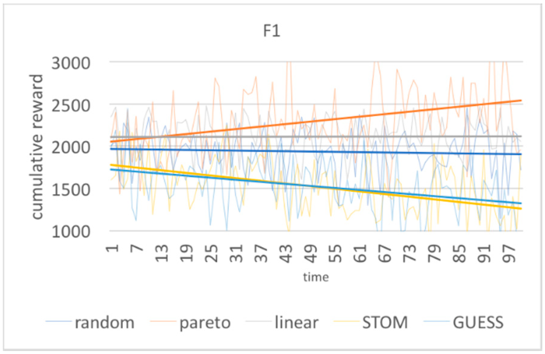
The results are consistent with what would we should expect from MORL. The final reward for a game increases as the defender learns with each iteration. Figure 2, Figure 3, Figure 4, Figure 5 and Figure 6 show the results over time for one starting network. From Figure 2, it is clear that not all the optimization approaches outperform a random strategy. Linear scalarization and the Pareto-Q-learning approach lead to better results over time, while the STOM and GUESS method do not lead to better results. Both STOM and GUESS prioritize fitting the goal prioritization over improving the results of the interaction.

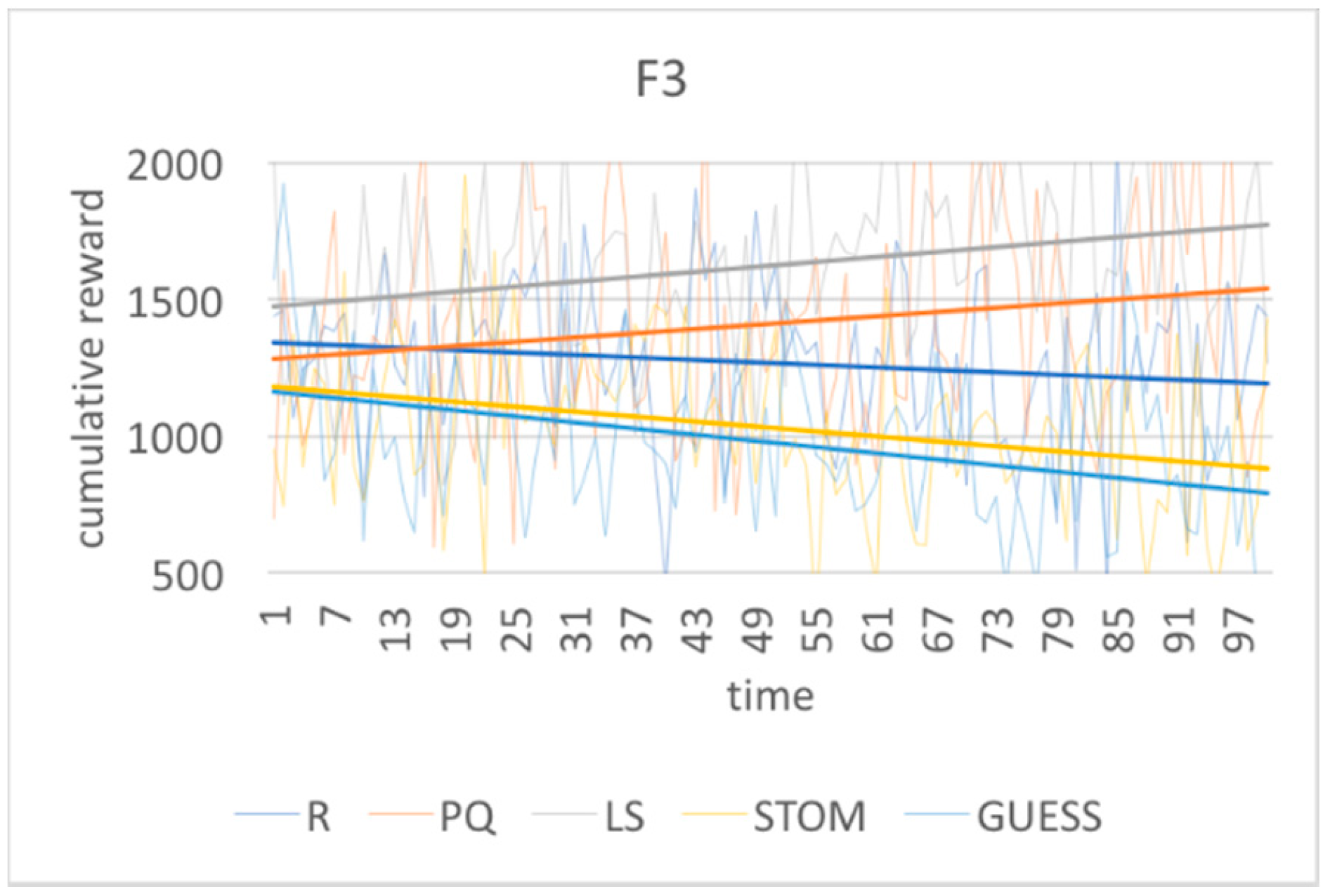
From Figure 3, Figure 4 and Figure 5, we can see that all the algorithms start with an unfavorable distribution of the goals. Both STOM and GUESS aggressively react by decreasing the results for goals f⁽¹⁾ and f⁽³⁾ and increasing the result for f⁽²⁾, until the algorithm reaches a goal distribution that matches the set goal prioritization of 3:7:2. The GUESS method slightly outperforms the STOM method.

The Pareto-Q-learning approach attempts increase the result for all goals. It does so by focusing on increasing the contribution of f⁽²⁾, while not to decreasing the results of f⁽¹⁾ and f⁽³⁾. Due to this, the goal distribution of Pareto-Q-learning falls well short of the desired 3:7:2 goal prioritization. The linear scalarization approach indiscriminately focuses on increasing the final scalarized result. This leads to a goal distribution which is lower than that of the Pareto-Q-learning approach, but still reasonably high, as the scalarization weights are the exact same as the goal prioritization.

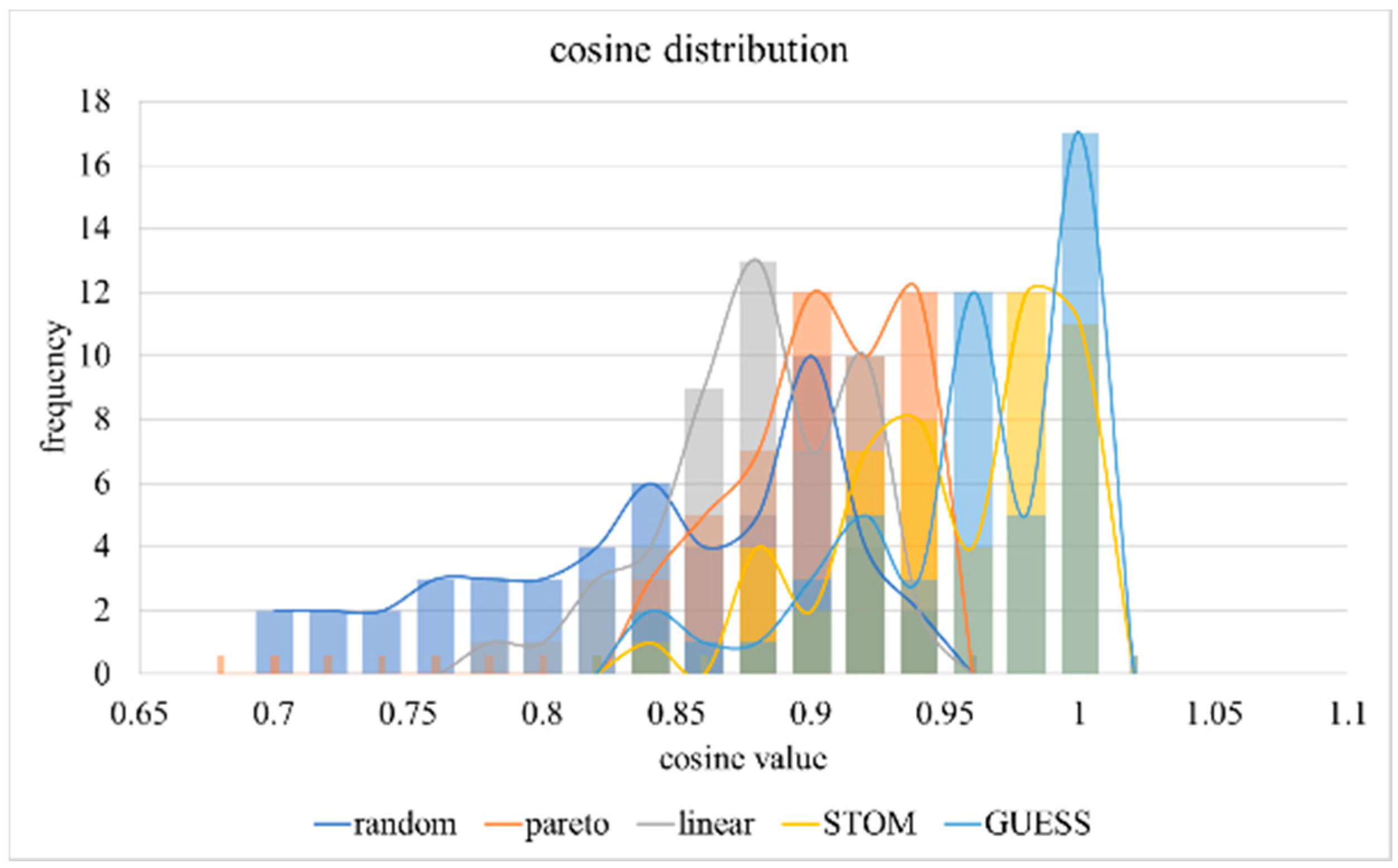
Figure 6 shows the cosine of the angle between the goal prioritization vector (3:7:2) and the result vector over time. This is according to Equation (25). A result vector parallel to the goal prioritization vector will have a cosine value of 1 and a result vector perpendicular to the goal prioritization vector will have a cosine value of 0. The results in Figure 6 make it obvious that the GUESS method is a superior approach for goal prioritization. With the exception of random choice, linear scalarization performs the worst.

$$\cos \theta =\frac{\overrightarrow{f_t}·\overrightarrow{p}}{\Vert \overrightarrow{f_t}\Vert \ast \Vert \overrightarrow{p}\Vert }$$

(25)

These results show a single game network. Different starting conditions may have different results.

4.4.2. Multiple Game Analysis

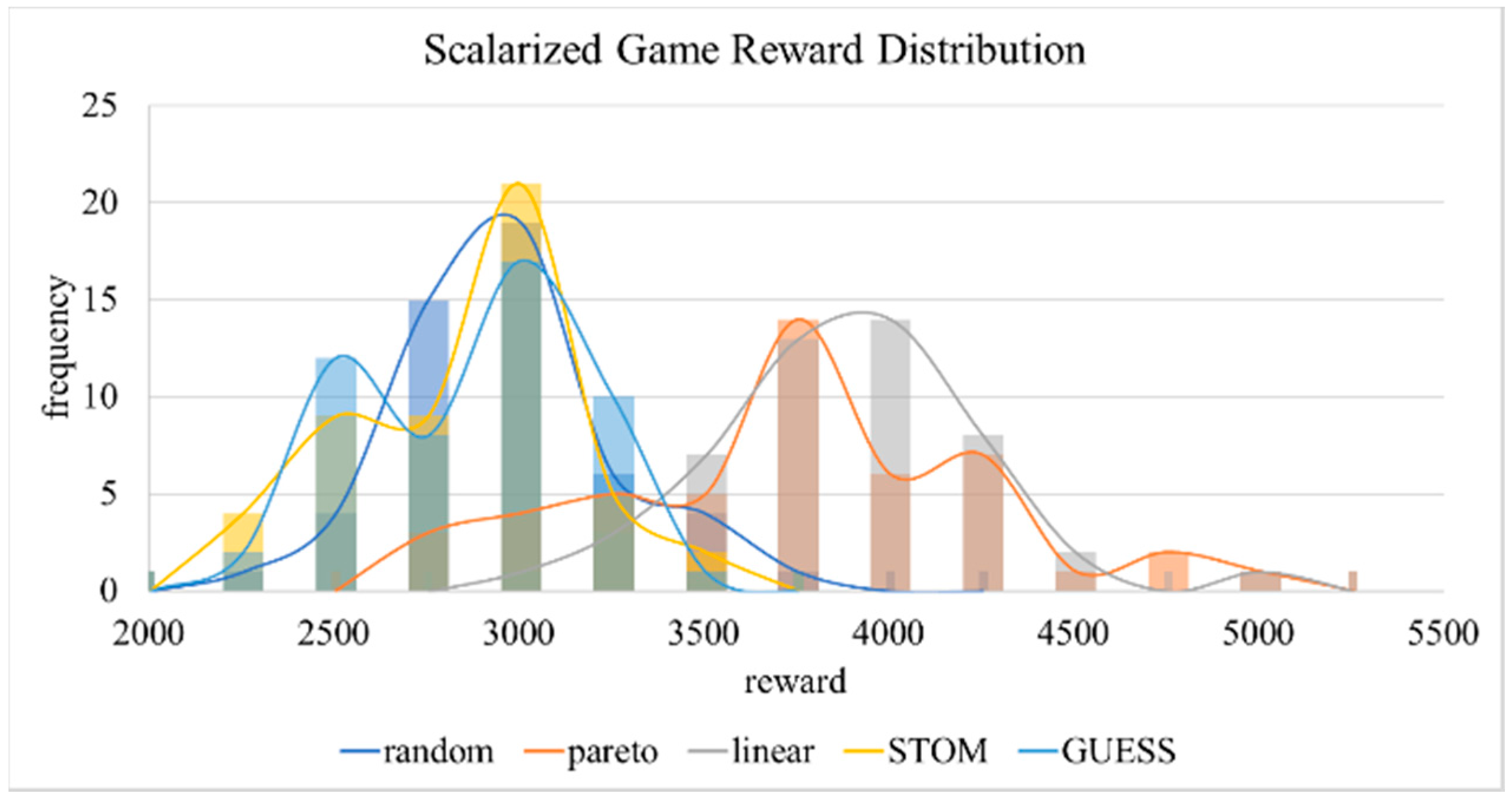
We determined if these results exist across starting conditions by mapping out the rewards over 50 different starting networks and statistically analyzing the resulting reward distribution.

Table 2. Multiple game analysis results.

		Mean	Std. Dev.	99% C.I.	t-Test
Game rewards	Random	2827.32	294.96	±107.45	2.03 × 10−14
	Pareto-Q-learning	3707.52	627.66	±228.66	-
	Linear scalarization	3727.16	405.20	±147.61	0.853
	STOM	2754.14	317.25	±115.58	9.60 × 10−16
	GUESS	2733.68	302.934	±110.36	2.20 × 10−16
f(1)/f(2) ratio	Random	0.831	0.066	±0.024	2.77 × 10−17
	Pareto-Q-learning	0.894	0.032	±0.012	1.71 × 10−16
	Linear scalarization	0.870	0.036	±0.013	2.24 × 10−21
	STOM	0.939	0.051	±0.019	0.016
	GUESS	0.945	0.050	±0.018	0.057

shows the mean, standard deviation, and 99% confidence interval for the scalarization of the cumulative game rewards and the cosine value of the game rewards. The table also includes the result of a t-test comparing the game rewards of the Pareto-Q-learning with that of the other approaches; and the results of a t-test comparing the cosine value of each approach to the desired value of 1. A graphical representation of these distributions is visible in Figure 7 and Figure 8.

The results show that Pareto-Q-learning and linear scalarization consistently outperform the other approaches for the cumulative rewards. A standard t-test, with a p-value of 0.05, confirms this difference. Linear scalarization performs comparable to Pareto-Q-learning with a t-statistic of 0.853. STOM and GUESS perform very poorly with results comparable to a random strategy selection. If the defender aims to merely maximize the game rewards, regardless of which goals are prioritized, the Pareto-Q-learning approach or linear scalarization give the best results.

The cosine results, however, show that Pareto-Q-learning and linear scalarization achieve this high cumulative result by ignoring the defender’s desired goal prioritization. The STOM and GUESS approaches meanwhile result in a goal distribution which is close to the optimum. The GUESS distribution is statistically not different from the desired goal prioritization. The standard t-test confirms this with GUESS t-statistic of 0.057, being the only one to exceed the p-value of 0.05. It is noteworthy that the STOM method led to a ratio that was still close to the desired goal prioritization, while the other approaches were nowhere near the distribution.

The results clearly show that if the defender wishes to have control over goal prioritization, the GUESS approach is the best. However the fairer distribution of rewards may not be worth the loss in cumulative rewards. The Pareto-Q-learning approach still appears to strike the best balance between the conflicting goals, with a high cumulative reward and a respectable goal distribution.

4.4.3. Complexity Analysis

We use the method proposed in [39] to calculate the Pareto fronts. The best-case complexity is $O\left(n\log n\right)$ and the worst-case complexity is $O(m{\left(n\right)}^2)$. The worst-case complexity linear scalarization is $O\left(n\right)$.

We tested the algorithm efficiency by recording the running time of just the optimization algorithm for each of 50 starting network conditions. The resulting time for 2000 operations is listed in

Table 3. Running time analysis.

	Running Times (in Seconds)
	Mean	Std. Dev.	99% C.I.
Pareto-Q-learning	2.5036	0.2118	±0.0772
Linear scalarization	0.0033	0.00039	±0.00014
STOM	0.0065	0.00005	±0.00002
GUESS	0.0079	0.00060	±0.00022

. Figure 9 shows the distribution of the running times. It is clear from the results that the Pareto-Q-learning is the most inefficient approach. By contrast, linear scalarization is the most efficient and runs 760 times faster than Pareto-Q-learning approach and two times faster than the other two scalarization approaches. Of the two algorithms in the middle, the STOM approach performs significantly better than the GUESS approach. These results confirm our assumption that the scalarization approaches outperform the Pareto-Q-Learning approach.

4.4.4. PDSSS System Analysis

We have researched and developed a Pareto Defense Strategy Selection Simulator (PDSSS) system for assisting network administrators on decision-making, specifically, on defense strategy selection.

The objective of the system is to develop a system that addresses the multi-criteria decision making using Pareto efficiency. The purpose is to assist network security managers in choosing a defense strategy to mitigate the damage to the business by an attack.

Our system is developed by specifically focusing on one specific type of attack, the network flooding attack. However, with slight changes the system should work with any attack that has multiple objectives. The goals, tasks, and solutions of PDSSS are listed below in

Table 4. System tasks and requirements.

#	Goals	Tasks	Sub-Task	Solutions
1	System Initialization	Topology configuration	Node attributes setting	Data import/Manual user import
			Connections/Edge configuration Sparsity	Data import/Manual user import
		Goal definition	Service cost setting	Boot strapping
		Agent initial configuration	Attacker point settingDefender point settings	Boot strapping
2	Simulate the agent actions	Attacker behavior		Randomized behavior
		Defender behavior	Static selection	Pareto Set method
			Machines Learning	Pareto-Q-learning
			Machine Learning Comparison	Scalarization
3	Output	Suggested strategies	For each selection method	UI: List of Strategies
		Final State	Topology of the network	UI: Graph UI: Brief text description

.

The GUI (Graphical User Interface) layout is visible in the wireframe in Figure 10, which consists of five sections:

-

The configuration panel

Here the user can choose the input configuration of the model. There are three models, each of which has a different set of goal functions.

-

The goal function before the application of optimization

Here the user can see the solution space for the goal functions before we implement the algorithm (i.e., the results from selecting a strategy as defined by the model).

-

The goal function after the application of optimization

Here the user can see the solution space for the goal functions after we implement the algorithm (i.e., the results from selecting a strategy as defined by the model).

-

The results

Here the user sees a summary of what the optimization algorithm has done for a single step.

-

The command buttons

Here the user interacts with the GUI by generating a new model with the given configuration or by loading an existing model from a csv (Comma-Separated Values) file.

In order to validate the proposed models using simulated results, we use the SNAP email-EU-core network dataset to extract the network topology. The network dataset in

Table 5. Dataset statistics.

Nodes	1005
Edges	25,571
Average clustering coefficient	0.3994
Number of triangles	105,461
Fraction of closed triangles	0.1085
Diameter (longest shortest path)	7
90-percentile effective diameter	2.9

contains email data from a large European research institution. The edge (u, v) represents the existence of an email communication between two users. The primary reason we use this data is that it has the properties of a peer-to-peer network presented in the models. Additionally, the higher clustering coefficient and higher number of triangles in the network allows us to easily extract smaller subgraphs to perform simplified versions of the simulations. Moreover, data contains a ‘ground-truth’ community membership of the nodes. Each node can only belong to one of the 42 departments. This makes it easy for us to classify nodes into high-value nodes and low-value nodes based on the department number. In addition to this, email services are often the victims of real-world DDOS attacks, which makes the dataset a relevant representation of the network model. The following tables detail the dataset.

Note that the dataset does not contain all the necessary information for the models in the simulations. The missing configuration data has been auto-generated.

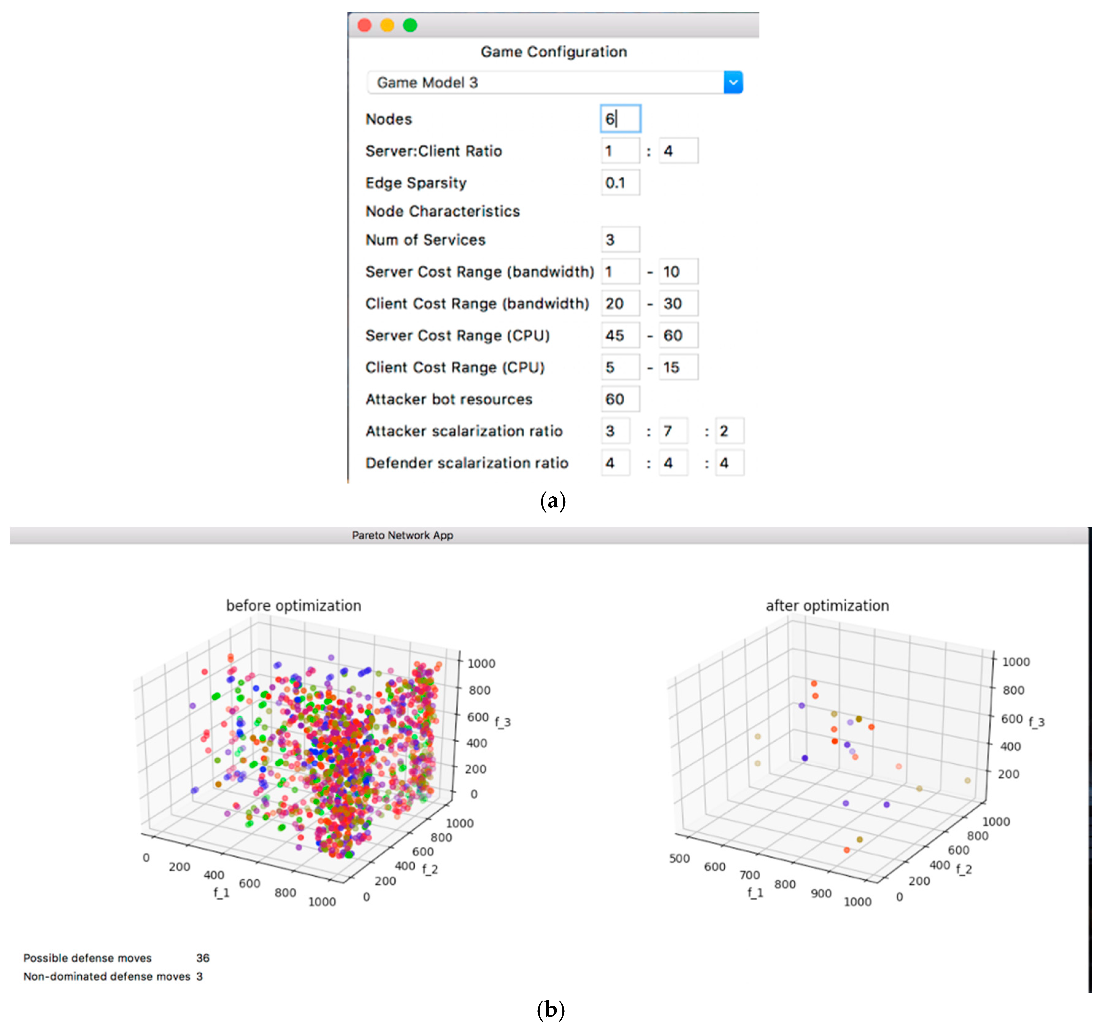
The PDSS system overview is shown in Figure 11, which is under the configuration of

Table 6. Configuration for a simple network.

Network Attributes	Bandwidth	CPU Resources
Can be compromised	3	3
High value nodes	1:10	45:60
Low value nodes	20:30	5:15
(high:low) value node ratio	1:4
Number of nodes	50
Attacker bot resources	60
Edge sparsity	0.01
Attacker scalarization	7:3:2
Defender scalarization	4:4:4

, and the user can select the regular network graph definition features: the number of nodes and server-client ratio. The user can select the model specific graph definition features: edge sparsity and cost ranges for bandwidth and CPU resources. The user can select the model features: attack resources and the scalarization ratios for the attacker and defender. The number of possible strategies is determined by the model. This model has a 3-D solution space.

In the first graph in Figure 11, it is difficult to visually identify the best strategies from the initial graph as most of the colors are spread across the graph. However, there is a noticeable concentration at the top-right corner of the graph.

On the second graph, the optimal values are much easier to interpret. The orange (~600, ~950, <650) and blue points are much more vivid than the khaki points, indicating higher scores in the goal functions. The orange and blue points are diagonally oriented from the inner upper left corner to the outer bottom right corner. This explains why these colors are brighter at the center. The other optimal values scattered near the walls are faint, indicating they score very low in one of the goals, although they are in the optimal set.

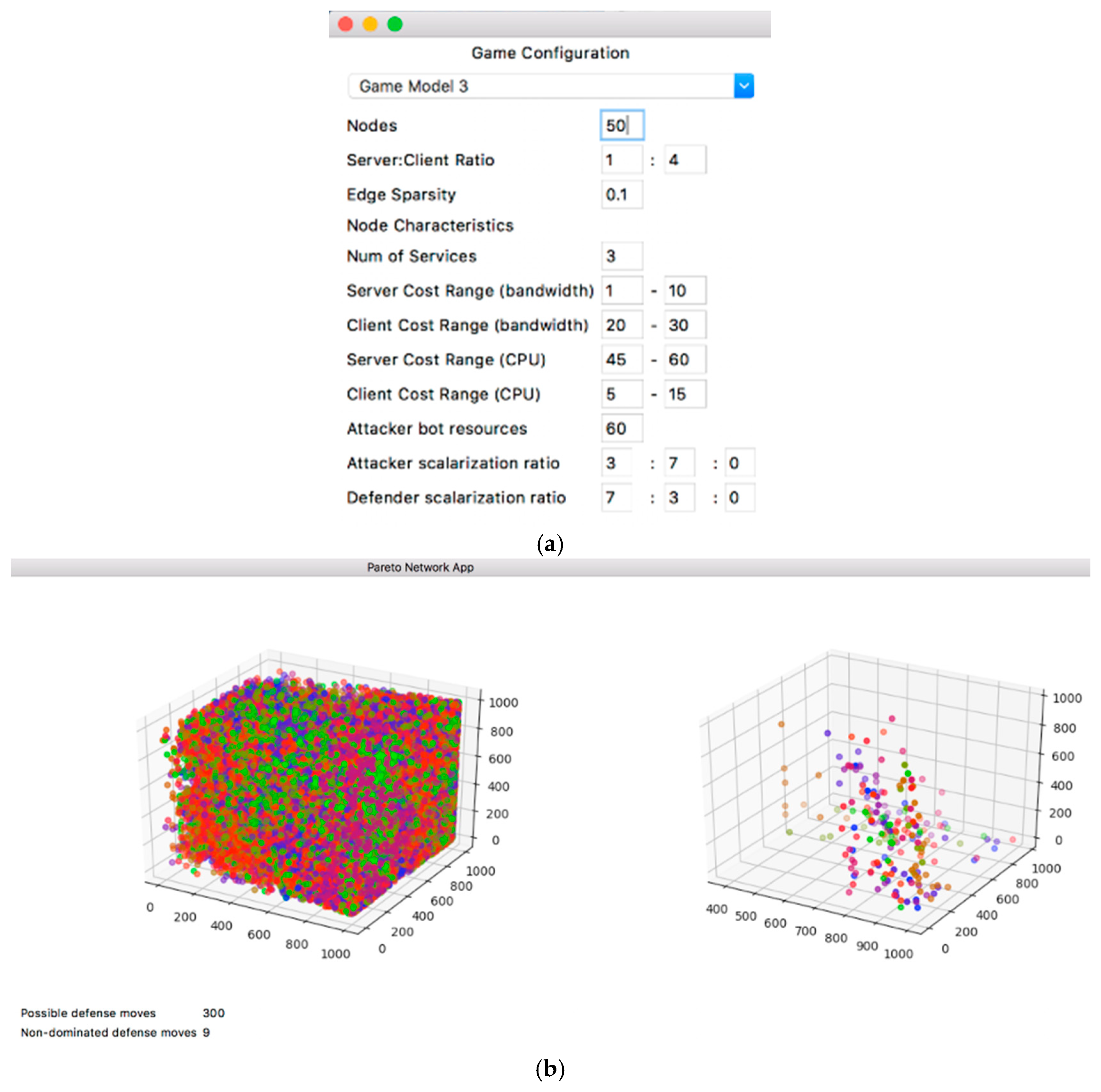
Figure 12 shows the PDSS system with a more realistic network size with configuration in

Table 7. Configuration for a complex network.

Network Attributes	Bandwidth	CPU Resources
Can be compromised	3	3
High value nodes	1:10	45:60
Low value nodes	20:30	5:15
(high:low) value node ratio	1:4
Number of nodes	50
Attacker bot resources	60
Edge sparsity	0.01
Attacker scalarization	7:3:2
Defender scalarization	4:4:4

. As is visible from the image, the graphical representation of the results is no longer useful. The algorithm also took much longer to graph the results. For the actual running of the experiments (which includes many repetitions), we opted not to use the GUI and instead ran the code from the command line.

In the first graph in the above figure, the initial strategies are cramped into the plot making it nearly impossible make an inference solely from the graph. However, the second graph shows the optimal non-dominated strategies. It is much easier for a DM to make a decision in this case just by referring to the second graph: all of the unnecessary dominated strategies have been removed. It seems green is the most distributed strategy, while blue and orange have fewer options.

5. Conclusions

This article shows that in network defense games, the Pareto-Q-learning approach suggested by Sun et al. leads to higher game rewards than scalarization approaches. However, those higher rewards are achieved by choosing actions that do not fully adhere to the defender’s desired goal distribution. It is possible to obtain a better goal distribution by choosing a scalarization approach that prioritizes the goal distribution over the final game reward.

The conducted experiment shows that for an abstract DDOS attack represented in the game model, this approach allows decision-makers to learn how best to allocate scarce resources to avoid a loss of service availability. The abstract DDOS model can be implemented with a decision-maker specific goal function. Various decision-makers can, thus, use the model to create a goal prioritization strategy specific to their network.

Our research in multi-criteria decision-making techniques has shown that scalarization is more efficient and less dependent on qualitative analysis than other options, such as the Analytical Hierarchy Process or the Tabular method. The experiment also shows that Pareto optimization may be computationally too expensive for real-time monitoring and response. However, the effectiveness of the algorithm can be significantly increased by the use of a scalarization function.

The usage of a reinforcement learning algorithm is also very apparent, as the algorithm produces better results over time. This means that the algorithm is very suited for offline learning. By gathering data on previous attacks, we can teach the algorithm to perform better than non-learning algorithms which cannot leverage that information.

We suggest that network defense games that wish to find an optimal solution via a MORL use the STOM approach, as this method leads to results that are within one standard deviation of the Pareto-Q-learning approach, while adhering closely to the desired goal distribution. The STOM method is also significantly more efficient than the Pareto-Q-learning approach.

References

- Montesino, R.; Fenz, S. Automation possibilities in information security management. In Proceedings of the 2011 European Intelligence and Security Informatics Conference (EISIC), Athens, Greece, 12–14 September 2011; pp. 259–262. [Google Scholar]
- Tsiropoulou, E.E.; Baras, J.S.; Papavassiliou, S.; Gang, Q. On the Mitigation of Interference Imposed by Intruders in Passive RFID Networks. In Proceedings of the International Conference on Decision and Game Theory for Security, New York, NY, USA, 2–4 November 2016. [Google Scholar]
- Cai, S.; Li, Y.; Li, T.; Deng, R.H.; Yao, H. Achieving high security and efficiency in RFID-tagged supply chains. Int. J. Appl. Cryptogr. 2010, 2, 3–12. [Google Scholar] [CrossRef]
- Tsiropoulou, E.E.; Baras, J.S.; Papavassiliou, S.; Sinha, S. RFID-based smart parking management system. Cyber-Phys. Syst. 2017, 3, 1–20. [Google Scholar] [CrossRef]
- Tsiropoulou, E.E.; Paruchuri, S.T.; Baras, J.S. Interest, Energy and physical-aware coalition formation and resource allocation in smart IoT applications. In Proceedings of the 2017 51st Annual Conference on Information Sciences and Systems, Baltimore, MD, USA, 22–24 March 2017; pp. 1–6. [Google Scholar]
- Van Moffaert, K.; Nowé, A. Multi-objective reinforcement learning using sets of pareto dominating policies. J. Mach. Learn. Res. 2014, 15, 3483–3512. [Google Scholar]
- Sun, Y.; Xiong, W.; Yao, Z.; Moniz, K.; Zahir, A. Network Defense Strategy Selection with Reinforcement Learning and Pareto Optimization. Appl. Sci. 2017, 7, 1138. [Google Scholar] [CrossRef]
- Kursawe, F. A variant of evolution strategies for vector optimization. In Proceedings of the International Conference on Parallel Problem Solving from Nature; Springer: Berlin/Heidelberg, Germany, 1990; pp. 193–197. [Google Scholar]
- Mariano, C.E.; Morales, E.F. Distributed reinforcement learning for multiple objective optimization problems. In Proceedings of the 2000 Congress on Evolutionary Computation, La Jolla, CA, USA, 16–19 July 2000; pp. 188–195. [Google Scholar]
- Cheng, F.Y.; Li, D. Genetic algorithm development for multiobjective optimization of structures. AIAA J. 1998, 36, 1105–1112. [Google Scholar] [CrossRef]
- Roijers, D.M.; Whiteson, S.; Vamplew, P.; Dazeley, R. Why Multi-objective Reinforcement Learning? In Proceedings of the European Workshop on Reinforcement Learning, Lille, France, 10–11 July 2015. [Google Scholar]
- Lizotte, D.J.; Bowling, M.; Murphy, S.A. Efficient Reinforcement Learning with Multiple Reward Functions for Randomized Controlled Trial Analysis. In Proceedings of the 27th International Conference on Machine Learning (ICML-10), Haifa, Israel, 21–24 June 2010. [Google Scholar]
- Zitzler, E.; Deb, K.; Thiele, L. Comparison of multiobjective evolutionary algorithms: Empirical results. Evol. Comput. 2000, 8, 173–195. [Google Scholar] [CrossRef] [PubMed]
- Zeleny, M. Multiple Criteria Decision Making (MCDM): From Paradigm Lost to Paradigm Regained? J. Multi-Criteria Decis. Anal. 2011, 89, 77–89. [Google Scholar] [CrossRef]
- Sutton, R.S.; Barto, A.G. Reinforcement Learning: An Introduction; MIT Press: Cambridge, MA, USA, 2011. [Google Scholar]
- Lu, F.; Chen, C.R. Notes on Lipschitz Properties of Nonlinear Scalarization Functions with Applications. Abstr. Appl. Anal. 2014, 2014, 792364. [Google Scholar] [CrossRef]
- Vamplew, P.; Yearwood, J.; Dazeley, R.; Berry, A. On the limitations of scalarisation for multi-objective reinforcement learning of pareto fronts. AI 2008 Adv. Artif. Intell. 2008, 5360, 372–378. [Google Scholar]
- Hiriart-Urruty, J.B. Tangent cones, generalized gradients and mathematical programming in Banach spaces. Math. Oper. Res. 1979, 4, 79–97. [Google Scholar] [CrossRef]
- Göpfert, A.; Riahi, H.; Tammer, C.; Zalinescu, C. Variational Methods in Partially Ordered Spaces; Springer Science & Business Media: Berlin/Heidelberg, Germany, 2006. [Google Scholar]
- Srinivas, N.; Deb, K. Muiltiobjective optimization using nondominated sorting in genetic algorithms. Evol. Comput. 1994, 2, 221–248. [Google Scholar] [CrossRef]
- Deb, K.; Pratap, A.; Agarwal, S.; Meyarivan, T. A fast and elitist multiobjective genetic algorithm: NSGA-II. IEEE Trans. Evol. Comput. 2002, 6, 182–197. [Google Scholar] [CrossRef]
- Zhou, A.; Qu, B.-Y.; Li, H.; Zhao, S.-Z.; Suganthan, P.N.; Zhang, Q. Multiobjective evolutionary algorithms: A survey of the state of the art. Swarm Evol. Comput. 2011, 1, 32–49. [Google Scholar] [CrossRef]
- Miettinen, K.; Mäkelä, M.M. On scalarizing functions in multiobjective optimization. OR Spectr. 2002, 24, 193–213. [Google Scholar] [CrossRef]
- Benayoun, R.; de Montgolfier, J.; Tergny, J.; Laritchev, O. Linear programming with multiple objective functions: Step method (STEM). Math. Program. 1971, 1, 366–375. [Google Scholar] [CrossRef]
- Miettinen, K. Nonlinear Multiobjective Optimization, Volume 12 of International Series in Operations Research and Management Science; Kluwer Academic Publishers: Dordrecht, The Netherland, 1999. [Google Scholar]
- Gábor, Z.; Kalmár, Z.; Szepesvári, C. Multi-criteria Reinforcement Learning. In Proceedings of the Fifteenth International Conference on Machine Learning, San Francisco, CA, USA, 24–27 June 1998; pp. 197–205. [Google Scholar]
- Barrett, L.; Narayanan, S. Learning all optimal policies with multiple criteria. In Proceedings of the 25th international conference on Machine learning, Helsinki, Finland, 5–9 July 2008; pp. 41–47. [Google Scholar]
- Roijers, D.M.; Vamplew, P.; Whiteson, S.; Dazeley, R. A survey of multi-objective sequential decision-making. J. Artif. Intell. Res. 2013, 48, 67–113. [Google Scholar]
- Li, Y. Deep reinforcement learning: An overview. arXiv, 2017; arXiv:1701.07274. [Google Scholar]
- Bellman, R. Dynamic Programming; Princeton University Press: Princeton, NJ, USA, 2010. [Google Scholar]
- Van Moffaert, K. Scalarized Multi-Objective Reinforcement Learning: Novel Design Techniques. In Proceedings of the 2013 IEEE Symposium on Adaptive Dynamic Programming and Reinforcement Learning (ADPRL), Singapore, 16–19 April 2013. [Google Scholar]
- Saaty, T.L. How to make a decision: The analytic hierarchy process. Eur. J. Oper. Res. 1990, 48, 9–26. [Google Scholar] [CrossRef]
- Sushkov, Y. Multi-Objective Optimization of Multi-Regime Systems; Digital System Architecture; Moscow State University: Moscow, Russia, 1984; pp. 21–24. [Google Scholar]
- Buchanan, J.; Gardiner, L. A Comparison of Two Reference Point Methods in Multiple Objective Mathematical Programming. Eur. J. Oper. Res. 2003, 149, 17–34. [Google Scholar] [CrossRef]
- Kasimoğlu, F.; Amaçlı, Ç.; Verme, K. A Survey on Interactive Approaches for Multi-Objective Decision Making Problems. Defence Sci. J. 2016, 15, 231–255. [Google Scholar]
- Zargar, S.T.; Joshi, J.; Tipper, D. A survey of defense mechanisms against distributed denial of service (DDoS) flooding attacks. IEEE Commun. Surv. Tutor. 2013, 15, 2046–2069. [Google Scholar] [CrossRef] [Green Version]
- Mirkovic, J.; Reiher, P. A taxonomy of DDoS attack and DDoS defense mechanisms. ACM SIGCOMM Comput. Commun. Rev. 2004, 34, 39–53. [Google Scholar] [CrossRef]
- Tian, X.; Fei, S. Robust control of a class of uncertain fractional-order chaotic systems with input nonlinearity via an adaptive sliding mode technique. Entropy 2014, 16, 729–746. [Google Scholar] [CrossRef]
- Mishra, K.K.; Harit, S. A Fast Algorithm for Finding the Non Dominated Set in Multi objective Optimization. Int. J. Comput. Appl. 2010, 1, 35–39. [Google Scholar]
Figure 1.
Sample network with 10 nodes.
Figure 2.
Cumulative reward scalarization over time.
Figure 3.
Cumulative reward over time for f(1).
Figure 4.
Cumulative reward over time for f(2).
Figure 5.
Cumulative reward over time for f(3).
Figure 6.
Cosine of the angle between the results and the goal prioritization vector.
Figure 7.
Distribution of scalarized game rewards.
Figure 8.
Distribution of f(1)/f(2) ratio.
Figure 9.
Distribution of algorithm running times.
Figure 10.
GUI (Graphical User Interface) layout of the Pareto Defense Strategy Selection Simulator (PDSSS) system.
Figure 11.
PDSSS system overview. (a) Control panel; (b) Results display.
Figure 12.
PDSSS analysis for large scale network. (a) Control panel; (b) Results display.