Optimal Steady-State Range Prediction Filter for Tracking with LFM Waveforms


Department of Intelligent Systems Design Engineering, Toyama Prefectural University, Imizu, Toyama 939-0398, Japan
Appl. Sci. 2018, 8(1), 17; https://doi.org/10.3390/app8010017
Submission received: 31 October 2017
/
Revised: 13 December 2017
/
Accepted: 20 December 2017
/
Published: 23 December 2017
Abstract
:Featured Application
Moving object tracker for aircrafts, robots, and intelligent vehicles.
Abstract
This communication proposes a gain design method of an - filter with linear frequency-modulated (LFM) waveforms to achieve optimal range prediction (tracking) of maneuvering targets in steady-state. First, a steady-state root-mean-square (RMS) prediction error, called an RMS-index, is analytically derived for a constant-acceleration target. Next, a design method of the optimal gains that minimizes the derived RMS-index is proposed. Numerical analyses demonstrate the effectiveness of the proposed method, as well as producing a performance improvement over the conventional Kalman filter-based design method. Moreover, the theoretical relationship between range tracking performance and a coefficient for range-Doppler coupling of LFM waveforms is clarified. Numerical simulations using the proposed method demonstrate LFM radar tracking of maneuvering targets and prove the method’s effectiveness.
1. Introduction
Maneuvering-target tracking using laser, radar, and/or sonar is essential for monitoring systems in robots, aircrafts, and intelligent vehicles. For some applications in such technical fields, linear frequency-modulated (LFM) waveforms are used to improve the tracking accuracy in the range direction [1,2,3,4,5]. Known as range-Doppler coupling, the important consideration when using LFM waveforms is the error in the range measurement in relation to the Doppler effect [5]. Hence, Kalman [6,7] and - filters [8,9,10] based on the state equations that take range-Doppler coupling into account are used for the tracking of moving objects using LFM waveforms to reduce this type of error. In particular, the analysis of the - filter using LFM waveforms (LFM-- filter) is important because it theoretically clarifies the mathematical formulation of the steady-state performance indices of tracking systems and establishes design criteria of the filter [8,9,10,11].
The steady-state filter analysis that accounts for the effects of range-Doppler coupling is important in designing the tracking filter with LFM waveforms. Ref. [8] presents a theoretical analysis of the fundamental performance of the LFM-- filter and reveals the relationship between the coefficient of range-Doppler coupling and the steady-state tracking performance. Although Ref. [8] only considers random process noise associated with acceleration in modeling the motion, this investigation is extended to general process noise, which considers random velocities and random jerks, among others, as given in Ref. [9]. However, in these studies, the design strategy of the tracking filter is not clearly presented and an empirical design is required. Ref. [10] proposes a gain design method for the LFM - filter based on theoretical performance indices. In this design method, a design parameter called the deterministic tracking index is introduced. However, the paper optimizes the estimation error of range or range rate but the prediction performance is not optimized. Moreover, a steady-state Kalman filter is assumed in conventional studies. Therefore, the relationship between filter gains is limited to Kalman filter equations. This assumption does not lead to minimum prediction errors because the Kalman filter optimizes not the range prediction but the estimation of the state vector. For these reasons, the range prediction using the LFM - filter is not optimized.
In contrast, with respect to a general tracking filter (without LFM waveforms), our previous work [12,13] introduced an efficiency performance index called a root-mean-square (RMS)-index, which expresses the steady-state root-mean-square error in position (range) predictions. Using this index, we achieved accurate tracking compared with conventional gains determined based on the Kalman filter equations. It is believed that the application of the RMS-index to the LFM - filter resolves the above-mentioned problems.
In this communication, a gain design method used to compose an LFM - filter that minimizes the steady-state range prediction errors is proposed. The RMS-index of the LFM - filter is derived and the proposed design method is introduced using the results obtained. A theoretical analysis proves that, using the proposed method, a smaller steady-state tracking error is achieved compared with the conventional design method based Kalman filter. Moreover, an application of the proposed method to an LFM radar simulation is demonstrated to show its effectiveness.
2. Problem Definition and Conventional Filter Design
This section defines the tracking problem taking into regard the LFM waveforms assumed and summarizes briefly the conventional filter design methods and their problems.
2.1. - Filter for LFM Waveforms
We focus attention on a steady-state second-order tracking filter for moving objects tracked using LFM waveforms. Filter gains become fixed values in steady-state tracking; a fixed-gain second-order tracking filter is known as an - filter [9,10,13]. For LFM waveforms, a tracking of the range and range rate are considered along with range-Doppler coupling in range measurements. We investigate the range prediction performance using the - filter characterized by the coefficient of range-Doppler coupling.
The tracking filter invokes an iterative prediction and smoothing (update) process. The prediction process of the - filter is [14]::
where is the smoothed target range at time , T the sampling interval, the predicted range, the smoothed range rate, and the predicted range rate. The smoothing process of the - filter for the LFM waveforms is [8,9,10]:
where is the measured range, the coefficient of range-Doppler coupling, and and are fixed filter gains. and is expressed as [10]:
where and are the true range and range rate, the white noise associated with a Gaussian measurement with standard deviation of , and , , and are the carrier frequency, the pulse length, and the bandwidth of LFM waveform, respectively. becomes a negative value when a down-chirp waveform is used. Hence, corresponds to an up-chirp waveform and corresponds to a down-chirp waveform. We refer to the - filter assumed by Equations (1)–(4) as the LFM - filter.
The purpose of this communication is finding the optimal α and β values that achieves minimum errors for the range prediction in steady-state conditions. For simplicity, we assume that and are known and constant.
2.2. Conventional Filter Design Methods
Steady-state performance analysis and filter design of the LFM - filter have been investigated in some studies [8,9,10]. These conventional studies derive the optimal filter gains based on the Kalman filter equations because the - filter is approximated as a steady-state Kalman filter. In the conventional filter design, the following relationship between and in steady-state conditions is used [10]:
where
is the normalized coefficient of range-Doppler coupling. To apply relation (7) in gain design, the following two methods are proposed.
- Tracking-index-based method [8]: a well-known and useful design parameter is the tracking index, which is defined as [8,14]:where is the standard deviation of the process noise of the measurement model used in Kalman filter tracking [14]. Equation (9) is obtained by steady-state assumption for the Kalman filter using a random acceleration process noise [8]. In steady-state conditions, both the prediction and estimation error covariance matrices converge and the optimal gain relations are obtained using these fixed matrices in the Kalman filter equations. The value of determines and by Equations (7) and (9). In filter design, a suitable is selected empirically based on the assumed degree of maneuvering of targets.
- Maximum RMS error (RMSE)-based method [10]: the tracking index-based approach requires an empirical setting of . To resolve this problem, Jain and Blair [10] proposed the deterministic evaluation function and a design parameter to optimize the range estimation. Their proposed evaluation function corresponds to a maximum RMSE determined by a maximum target acceleration, which is defined as:where denotes the mean, the true range of the target undergoing constant acceleration, the steady-state variance of the range estimation error assuming only measurement noise, corresponds to the steady-state lag (bias error) for constant-acceleration target, and is called the deterministic tracking index defined using the maximum acceleration and ; these are expressed as:where is the maximum acceleration of the target. The optimal is determined by minimizing RMSE using Equation (7) and the known (i.e., and are known).
It is well known that the tracking index-based method is useful in the design of Kalman and - filters. However, an empirical setting for is required. The maximum RMSE-based approach automatically determines optimal and from . The setting of of is easily compared with because its physical meaning is clear. However, the two above-stated methods assume only random acceleration process noise in the Kalman filter equations [8,10]. The gain relation of Equation (7) is derived using this assumption. Although an arbitrary random motion parameter (not only acceleration but also velocity, for example) is assumed for process noise in [9], this study also assumes Kalman filter equations using white-Gaussian process noise. This means that the above conventional design methods are not optimal when other process noise is assumed (including situations where white-Gaussian process noise is not assumed). Moreover, the Kalman filter optimizes the estimation of the target state, whereas the prediction of the range is not optimized.
3. Proposed Optimal Range Prediction Filter Design
To resolve the problems arising with conventional approaches, this section proposes the optimal gain setting method to optimize range prediction. To achieve this, the RMS-index-based design approach that was proposed in previous work [13] is adapted to an LFM - filter. This approach can be considered as a modification of the maximum RMSE-based method for the minimization of errors in , and not for . Moreover, as the RMS-index-based approach does not require assuming process noise, the problems caused by the Kalman filter equations and described in the previous section do not exist.
3.1. RMS-Index for LFM - Filter
The RMS-index approach minimizes the RMSE of the prediction error of range (or position). In this section, the RMS-index is defined and derived for the LFM - filter. Similar to Equation (10), the RMS-index for the range prediction is defined as [13]:
where is the steady-state variance of the range prediction errors assuming only sensor noise and is the steady-state bias error of the range prediction assuming a target moving with constant acceleration . The RMS-index expresses the maximum RMS error for the prediction of the range (or position) in steady-state conditions. Because the LFM - filter is using the constant-velocity model as indicated in Equations (1) and (2), there is a bias error in the steady state associated with the accelerating target, and the filter diverges for the target moving with constant jerk. Thus, the maximum (worst-case) error for the steady-state LFM - filter is calculated by assuming the target moving with [10].
To derive , (steady-state variance of random errors) and (steady-state bias error) are calculated one by one. First, of the LFM - filter is calculated. There is no bias error associated with targets moving with constant velocity because the - filter uses the constant-velocity model. Hence, in the constant-velocity target tracking, there are only random errors arising from the radar measurement noise. These mean that is calculated by the mean square error for the constant-velocity target, and is calculated as
where is the true range of the target moving with constant velocity. Equation (15) contains the effects on sensor noise only and does not contain the errors resulting from differences between the model and the motion. The derivation of Equation (15) is given in Appendix A.
Next, is calculated as the bias error for the target for which the acceleration is . The bias error is the mean range prediction error in the steady-state, and is calculated from
The derivation of Equation (16) is given in Appendix B. Using the derived results of Equations (15) and (16), the RMS-index is calculated using Equation (14).
3.2. Filter Design Method
The optimal filter gains is obtained by minimization of RMSE. Therefore, using Equations (14)–(16), the evaluating function for the design filter gains is defined as
The optimal gains are calculated by solving the following optimization problem:
for which the constraints are the stability conditions of the LFM - filter [9].
Different from the conventional methods, the proposed method directly determines and by searching the minimum value of without using the gain relations derived from the Kalman filter equations, for example, Equation (7). Moreover, the Kalman filter equations are also not used in deriving . This means that the proposed method does not require the assumption of the process noise that limits the gain relation of the - filter. In addition, the proposed method minimizes not the errors in estimation () but those in prediction (), which is different from the Kalman filter. Therefore, the proposed method determines optimal filter gains with respect to the steady-state range prediction. Table 1 summarizes the features of the conventional and proposed design methods.
4. Performance Evaluation
We next investigate the performance of the LFM - filter with the proposed gain design method using theoretical steady-state analyses and numerical simulations assuming radar tracking of a maneuvering target. Both the proposed and the conventional maximum RMSE-based methods [10] are compared.
4.1. Theoretical Analysis
RMSE values calculated using Equations (14)–(17) of the conventional and proposed methods are compared for various and . We assume that and T are normalized to 1.
Figure 1 shows the relationship between and RMSE for = ±0.25 and ±0.5. For all instances, RMSE of the proposed method is smaller than that of the conventional method. For , although the performance of the proposed method is slightly better than that of the conventional method for relatively small , the performance difference becomes large for large . For , the performance difference between the conventional and proposed methods for relatively small is large compared with instances with .
Figure 2 shows the relationship between and RMSE for = 0.1 and 1. For tracking with LFM waveforms, range estimation accuracy deteriorates considerably for small (negative) [10], which is also a feature of results from conventional methods. However, the proposed method achieves relatively small tracking accuracy for . This is because it directly minimizes the range prediction errors without assuming the Kalman filter equations. The gain relation is limited to Equation (7) when we assume the random acceleration process noises in the Kalman filter equation of the conventional method. However, the optimal gains with respect to the range prediction calculated with the proposed method are not acquired from Equation (7). Moreover, Figure 2b shows that the tracking accuracy of the conventional method for also deteriorates around . The reason is that the optimal gains for the conventional methods are not effectively obtained as a consequence of the limited gain relation, Equation (7). These results theoretically verify that the proposed method achieves better tracking accuracy than the conventional RMSE-based method by the direct optimization of the range-tracking RMSE (the RMS-index) without using the Kalman filter equations.
4.2. LFM Radar Simulation
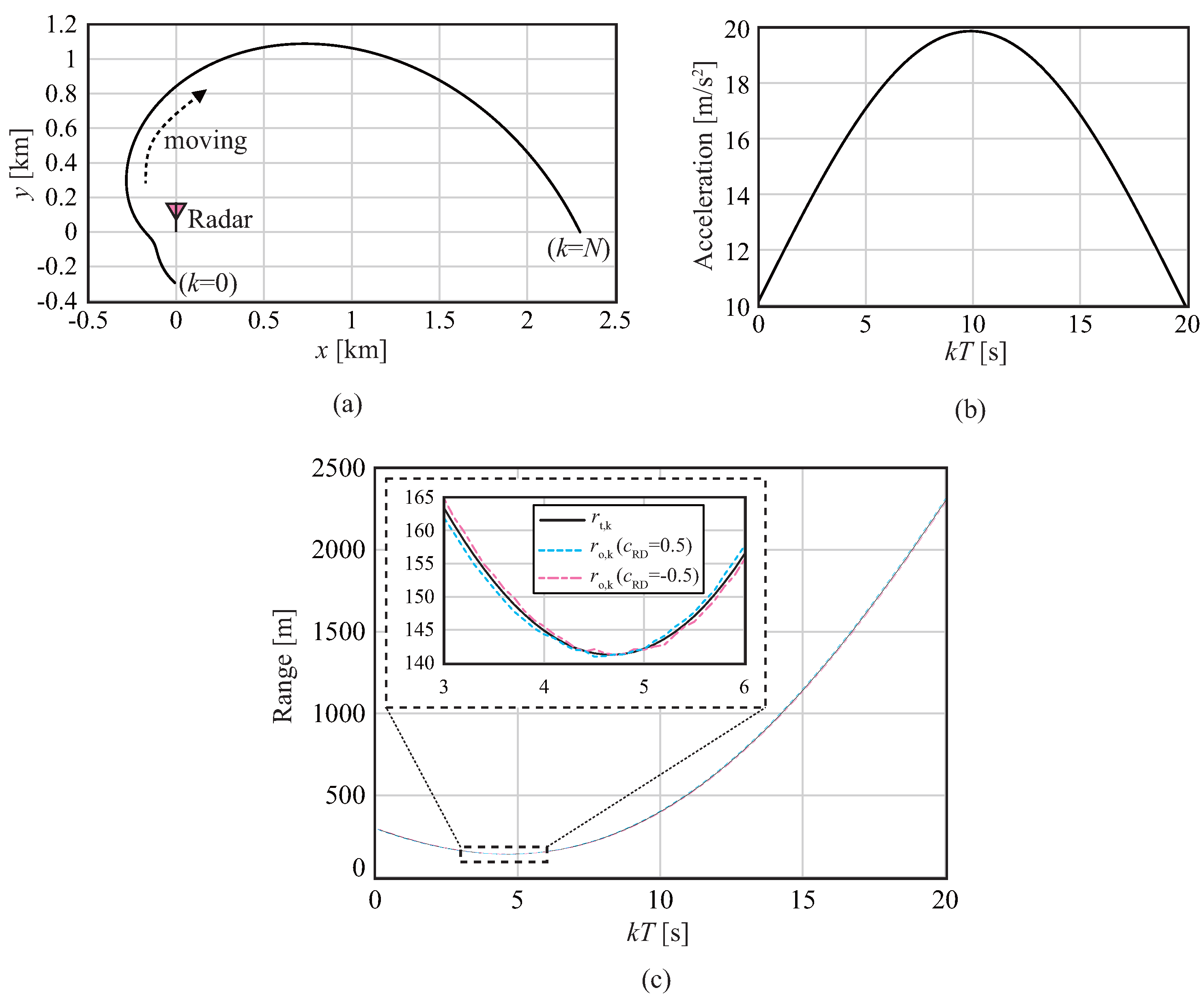
Finally, numerical simulation results are presented to demonstrate the effectiveness of the proposed method in range tracking using LFM radar. Figure 3 shows the simulation scenario. Although a two-dimensional problem is considered, we assume range measurements taken using a single LFM radar to demonstrate the validity of the proposed range tracking method for the target other than the constant-acceleration target assumed in the analysis. Figure 3a shows the true moving orbit of the target in the plane and the radar position. The true motion of the target in x and y are and , where is the number of samples with respect to k. In this setting, the true range in the simulation is =. The LFM radar is located at and its T is 0.1 s. Figure 3b shows the true acceleration of the target with respect to k. Based on this target acceleration, it is assumed that the approximate target maximum acceleration m/s has been obtained. Figure 3c shows the true and observed range data for = ±0.5 used as . Two instances = ±0.5 are considered and their standard deviations for measurement noise are both = 0.2 m. These settings give = 1.0 with Equation (13). We compared the RMS prediction errors of the conventional method of [10] and the proposed method for = ±0.5. As shown in Figure 3c, the range–offset dependence on is confirmed, and their effects on the range prediction accuracy when applying the conventional and proposed methods were investigated. The RMS prediction error at each time is calculated from one thousand Monte Carlo simulations; that is,
where is the predicted range in the m-th Monte Carlo simulation.
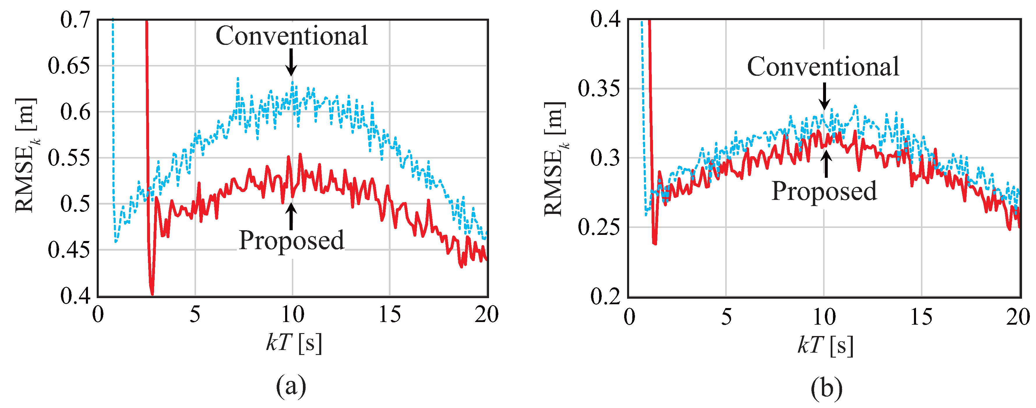
Figure 4 shows the simulation results for = ±0.5. For both instances, the proposed method achieves accurate tracking for steady states compared with the conventional method. In particular, the proposed method is effective around s because the filter gains are optimized for the maximum acceleration value. As shown in these results, the values of for = 0.5 is smaller than that for = −0.5. This is because that the positive supports the prediction process in the tracking filtering as fully discussed in [11]. Note that the relationship between the range prediction error and is also shown in Figure 2, and this also verifies the performance improvement when using positive . The performance difference between the conventional and proposed methods is relatively large for . The reason is that the range prediction accuracy has been already improved through the effect of positive [11] for = 0.5. Thus, the likelihood of an improvement using the proposed method is small. In contrast, for = −0.5, the range prediction errors widen with negative . Therefore, using the proposed method seems to compensate for these errors effectively. Therefore, the performance improvement with this method becomes relatively large for = −0.5. In terms of , although smaller values are achieved, the difference between the conventional and proposed methods is relatively small. However, the accuracy in steady-state tracking of the proposed method is always better than that of the conventional method. These results show the effectiveness of the proposed method for maneuvering targets (not only the targets with constant acceleration). In addition, the simulation results are consistent with the theoretical analysis described in the previous subsection.
5. Conclusions
This paper proposed a gain design method to achieve optimal steady-state range tracking for the LFM - filter. The RMS-index, which reflects the range prediction RMS errors in steady-state, was derived for the LFM - filter, and the gain design based on the minimization of the RMS-index was presented. The theoretical analyses proved that the proposed method generates smaller RMS errors in range tracking compared with that for the conventional method, which is based on the minimization of the RMS estimation error and the Kalman filter equations. The relationship between range-tracking performance and the important parameters (the normalized range-Doppler coupling coefficient) and (the design parameter called the deterministic tracking index) were also clarified. Moreover, numerical simulations employing LFM radar tracking verified the effectiveness of the proposed method. However, to clarify the performance of the proposed method in terms of the range prediction considering the range-Doppler coupling and the RMS-index, only theoretical analyses and ideal simulations were performed that did not account for various factors related to tracking accuracy, such as the multi-pass effect, signal distortion depending on the scattering characteristics of targets, directivity of the antenna, and multi-target cases. To apply LFM radar tracking with the proposed method in real environments, a comprehensive experimental study considering these foregoing effects and range-Doppler coupling is important work that remains.
Acknowledgments
This work was supported in part by the JSPS KAKENHI Grant No. 16K16093. I thank Richard Haase, Ph.D, from Edanz Group (www.edanzediting.com/ac) for editing a draft of this manuscript.
Conflicts of Interest
The author declares no conflict of interest.
Appendix A. Derivation of Equation (15)
Because is the true range of a target moving with constant velocity, this is expressed as
where is the true range rate. With Equations (1) and (A1), the variance of the range prediction error is found to be
Appendix B. Derivation of (16)
By simplifying these equations, and are related by
Because we have assumed that the maximum acceleration of the target is constant but do not assume measurement errors, the true and measured target positions are expressed as
where denotes the z-transform. With Equations (A10)–(A12), the predicted error in the z-domain, , is
References
- Guo, N.; Gao, C.; Xue, M.; Niu, L.; Zhu, S.; Feng, L.; He, H.; Cao, Z. Ranging method based on linear frequency modulated laser. Laser Phys. 2017, 27, 065108. [Google Scholar] [CrossRef]
- Zhang, Y.X.; Hong, R.J.; Yang, C.F.; Zhang, Y.J.; Deng, Z.M.; Jin, S. A Fast Motion Parameters Estimation Method Based on Cross-Correlation of Adjacent Echoes for Wideband LFM Radars. Appl. Sci. 2017, 7, 500. [Google Scholar] [CrossRef]
- Chua, M.Y.; Koo, V.C.; Lim, H.S.; Sumantyo, J.T.S. Phase-Coded Stepped Frequency Linear Frequency Modulated Waveform Synthesis Technique for Low Altitude Ultra-Wideband Synthetic Aperture Radar. IEEE Access 2017, 5, 11391–11403. [Google Scholar] [CrossRef]
- Othman, M.A.B.; Belz, J.; Farhang-Boroujeny, B. Performance Analysis of Matched Filter Bank for Detection of Linear Frequency Modulated Chirp Signals. IEEE Trans. Aerosp. Electron. Syst. 2017, 53, 41–54. [Google Scholar] [CrossRef]
- Bruno, L.; Braca, P.; Horstmann, J.; Vespe, M. Experimental Evaluation of the Range-Doppler Coupling on HF Surface Wave Radars. IEEE Geosci. Remote Sens. Lett. 2013, 10, 850–854. [Google Scholar] [CrossRef]
- Maresca, S.; Braca, P.; Horstmann, J.; Grasso, R. Maritime Surveillance Using Multiple High-Frequency Surface-Wave Radars. IEEE Trans. Geosci. Remote Sens. 2014, 52, 5056–5071. [Google Scholar] [CrossRef]
- Zhou, G.; Yu, C.; Cui, N.; Quan, T. A Tracking Filter in Spherical Coordinates Enhanced by De-noising of Converted Doppler Measurements. Chin. J. Aeronaut. 2012, 25, 757–765. [Google Scholar] [CrossRef]
- Wong, W.; Blair, W.D. Steady-state tracking with LFM waveforms. IIEEE Trans. Aerosp. Electron. Syst. 2000, 36, 701–709. [Google Scholar] [CrossRef]
- Amishima, T.; Ito, M.; Kosuge, Y. Stability condition and steady-state solution of various alpha-beta filters for linear FM pulse compression radars. Electron. Commun. Jpn. 2004, 87, 13–22. [Google Scholar] [CrossRef]
- Vineet, J.; Blair, W.D. Filter design for steady-state tracking of maneuvering targets with LFM waveforms. IIEEE Trans. Aerosp. Electron. Syst. 2009, 45, 296–300. [Google Scholar]
- Fitzgerald, R.J. Effects of Range-Doppler Coupling on Chirp Radar Tracking Accuracy. IEEE Trans. Aerosp. Electron. Syst. 1974, AES-10, 528–532. [Google Scholar] [CrossRef]
- Saho, K.; Masugi, M. Automatic Parameter Setting Method for an Accurate Kalman Filter Tracker Using an Analytical Steady-State Performance Index. IEEE Access 2015, 3, 1919–1930. [Google Scholar] [CrossRef]
- Saho, K.; Masugi, M. Performance Analysis and Design Strategy for a Second-Order, Fixed-Gain, Position-Velocity-Measured (alpha-beta-eta-theta) Tracking Filter. Appl. Sci. 2017, 7, 758. [Google Scholar] [CrossRef]
- Kalata, P.R. The Tracking Index: A Generalized Parameter for α-β and α-β-γ Target Trackers. IEEE Trans. Aerosp. Electron. Syst. 1984, AES-20, 174–182. [Google Scholar] [CrossRef]
Figure 1.
Relationship between and RMSE for 0.25 (a); 0.5 (b); −0.25 (c); and −0.5 (d).
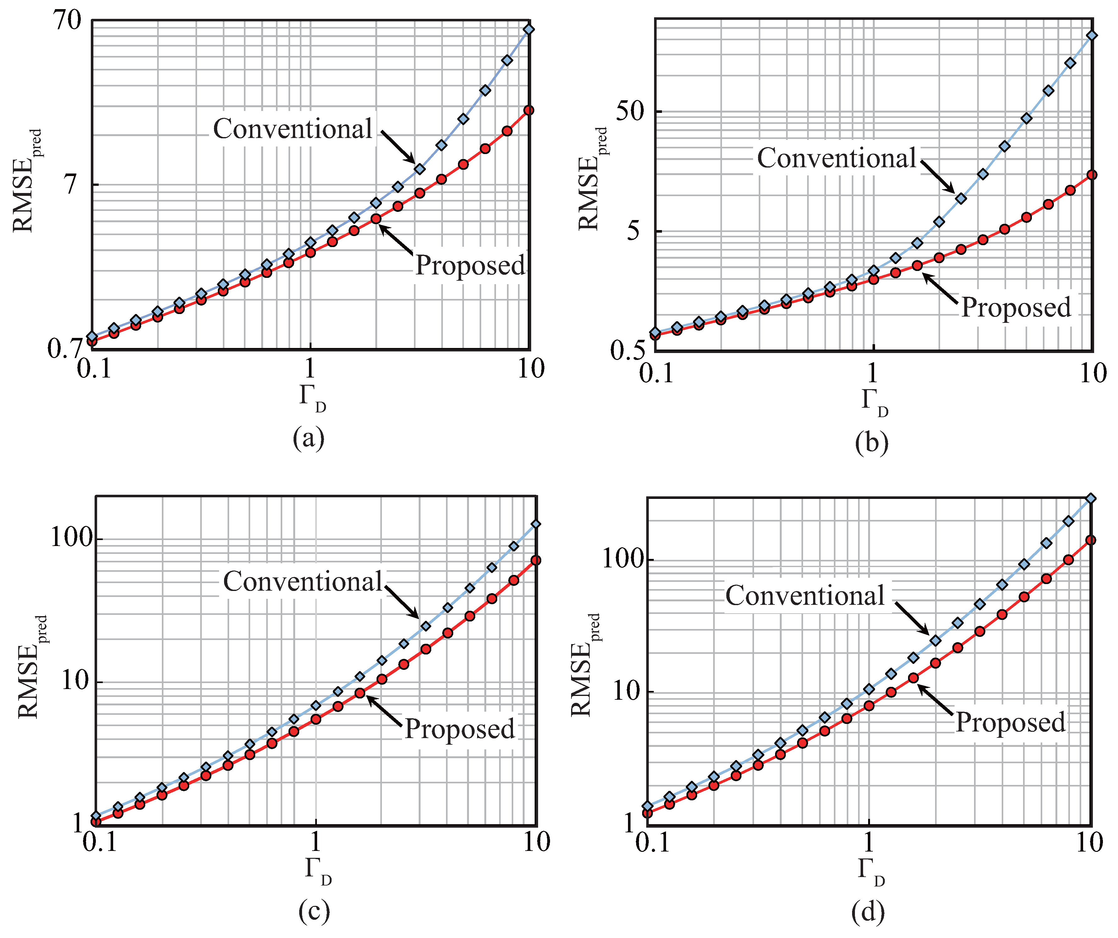
Figure 2.
Relationship between and RMSE for = 0.1 (a) and 1 (b).
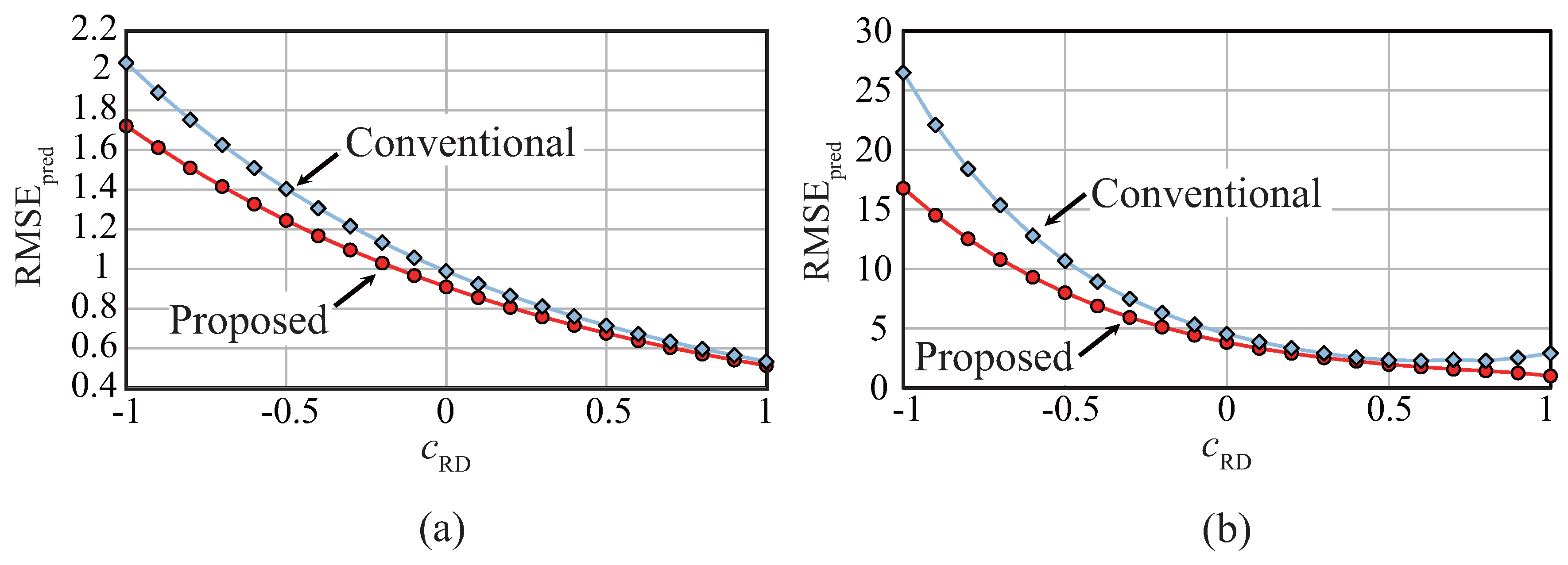
Figure 3.
Simulation scenario. (a) true orbit of the target and radar position; (b) true acceleration of the target; and (c) true and measurement range for .
Figure 3.
Simulation scenario. (a) true orbit of the target and radar position; (b) true acceleration of the target; and (c) true and measurement range for .

Figure 4.
Simulation results for = −0.5 (a) and 0.5 (b).


Table 1.
Summary of the conventional and proposed design methods.
| Design Methods | Preset Parameter | Evaluating Function | Process Noise |
|---|---|---|---|
| Tracking index-based method of [8] | Not used | Random acceleration | |
| Tracking index-based method of [9] | Not used | Arbitrary random parameter | |
| Maximum root mean square error (RMSE) [10] | Equations (10)–(12) | Random acceleration | |
| Proposed method | Equation (17) | Not assumed |
© 2017 by the author. Licensee MDPI, Basel, Switzerland. This article is an open access article distributed under the terms and conditions of the Creative Commons Attribution (CC BY) license (http://creativecommons.org/licenses/by/4.0/).
Share and Cite
MDPI and ACS Style
Saho, K. Optimal Steady-State Range Prediction Filter for Tracking with LFM Waveforms. Appl. Sci. 2018, 8, 17. https://doi.org/10.3390/app8010017
AMA Style
Saho K. Optimal Steady-State Range Prediction Filter for Tracking with LFM Waveforms. Applied Sciences. 2018; 8(1):17. https://doi.org/10.3390/app8010017
Chicago/Turabian StyleSaho, Kenshi. 2018. "Optimal Steady-State Range Prediction Filter for Tracking with LFM Waveforms" Applied Sciences 8, no. 1: 17. https://doi.org/10.3390/app8010017
Note that from the first issue of 2016, this journal uses article numbers instead of page numbers. See further details here.