
A Real-Time Sound Field Rendering Processor


1
RIKEN Advanced Institute for Computational Science, Kobe, Hyogo 650-0047, Japan
2
Research Center for Advanced Computing Infrastructure, Japan Advanced Institute of Science & Technology, Nomi, Ishikawa 923-1292, Japan
3
Department of Architecture and Architectural Engineering, Kyoto University, Kyoto 615-8540, Japan
4
Department of Electrical Engineering and Information Technology, Tohoku Gakuin University, Sendai, Miyagi 980-8511, Japan
5
Faculty of Science and Engineering, Doshisha University, Kyotanabe, Kyoto 610-0321, Japan
*
Author to whom correspondence should be addressed.
Appl. Sci. 2018, 8(1), 35; https://doi.org/10.3390/app8010035
Submission received: 3 November 2017
/
Revised: 5 December 2017
/
Accepted: 18 December 2017
/
Published: 28 December 2017
(This article belongs to the Special Issue Sound and Music Computing)
Abstract
:Real-time sound field renderings are computationally intensive and memory-intensive. Traditional rendering systems based on computer simulations suffer from memory bandwidth and arithmetic units. The computation is time-consuming, and the sample rate of the output sound is low because of the long computation time at each time step. In this work, a processor with a hybrid architecture is proposed to speed up computation and improve the sample rate of the output sound, and an interface is developed for system scalability through simply cascading many chips to enlarge the simulated area. To render a three-minute Beethoven wave sound in a small shoe-box room with dimensions of 1.28 m × 1.28 m × 0.64 m, the field programming gate array (FPGA)-based prototype machine with the proposed architecture carries out the sound rendering at run-time while the software simulation with the OpenMP parallelization takes about 12.70 min on a personal computer (PC) with 32 GB random access memory (RAM) and an Intel i7-6800K six-core processor running at 3.4 GHz. The throughput in the software simulation is about 194 M grids/s while it is 51.2 G grids/s in the prototype machine even if the clock frequency of the prototype machine is much lower than that of the PC. The rendering processor with a processing element (PE) and interfaces consumes about 238,515 gates after fabricated by the 0.18 µm processing technology from the ROHM semiconductor Co., Ltd. (Kyoto Japan), and the power consumption is about 143.8 mW.
1. Introduction
Sound field rendering exhibits numerical methods to model sound propagation behavior in spatial and time domains, and is fundamental to numerous scientific and engineering applications, which vary widely from interactive computer games and virtual reality to highly accurate computations for offline applications like architecture design. To date, many analysis algorithms, including geometric methods and wave-based methods, have already been proposed to analyze sound wave propagations. In particular, wave-based methods are popularly applied because of their high accuracy, in which a sound space is discretized into small grids, and an analysis algorithm is applied on each grid to model sound behavior at discrete time steps. Among wave-based methods, the finite difference time domain (FDTD) method has been widely applied and has become an essential algorithm in room acoustics owing to its ease of implementation and parallelization. FDTD was introduced to analyze acoustical behavior by O. Chiba et al., and D. Botteldooren et al. [1,2,3]. However, numerical dispersion is an inherent problem constraining the valid bandwidth in the FDTD method. To reduce numerical dispersion, L. Savioja et al., G.R. Campos et al., and D.T. Murphy et al. applied digital waveguide mesh topologies [4,5,6]; K. Kowalczyk and M. van Walstijn proposed a second-order accurate FDTD scheme, and the 27-point compact explicit FDTD scheme was introduced [7]. J. van Mourik and D. Murphy investigated a set of high-order explicit “large-star” stencils, which could obtain less dispersiveness at low frequencies and provide high valid bandwidth [8]. H. Brian and B. Stefan proposed the fourth-order accurate explicit and implicit FDTD schemes for 2D and 3D wave equations [9,10], respectively. They recently presented a set of two-step explicit FDTD schemes with high-order accuracy in both space and time for 3D wave equations [11].
On the other hand, since spatial grids are usually oversampled to suppress the numerical dispersion errors in the FDTD method [10], the memory usage and computing power required is significant. Generally, the computing power of solving such wave equations increases as the fourth power of frequency [12], and it is increased proportionally with the volume of sound spaces. For example, every doubling of the frequency band induces a 16-fold increase in the computational load [2]. Given the auditory range of humans (20 Hz–20 kHz), analyzing sound wave propagation in a space corresponding to a concert hall or a cathedral (e.g., volume of 10,000–15,000 m3) for the maximum simulation frequency of 20 kHz requires petaflops of computing power and terabytes of memory. As a result, the traditional sound rendering systems based on computer simulations demand huge computation power, especially for broadband simulations extending into the kilohertz range. They require a PC cluster or supercomputer for computations because of constraints of memory bandwidth and the performance of arithmetic units in a single PC. Although the performance of the arithmetic units can be enhanced through increasing the clock frequency of processors or using multicores, it is constrained by the power wall and dark silicon problems.
In recent years, general-purpose graphic processing units (GPGPUs) and FPGAs have been applied to speed up the arithmetic operations in sound rendering systems [13,14,15,16,17,18,19,20,21,22]. Although GPGPU-based solutions achieve high computation performance through increasing system threads, the input and output interfaces are more difficult to customize according to applications. Therefore, it is very hard to directly input the live signals and output the rendered results in such sound rendering systems in interactive and real-time applications. In some solutions, to apply GPGPUs in real-time sound rendering, the rendered results are sent to a buffer, and then the audio cards in the host machine are driven to output the rendered results through calling their application program interfaces (APIs). The constraint of these solutions is system scalability because the number of audio cards is limited by the number of peripheral component interconnect (PCI) slots inside the host machine. Especially in multi-channel applications, such as 128 channels, it is impossible to output using the audio cards inserted in the host machine, instead, the external professional equipment is required. Then, how to output the run-time rendered results from the GPGPU to the output equipment is a problem because no interfaces are provided to the external devices. In contrast, the input/output (I/O) interfaces can be customized in accordance to applications in FPGA. For multi-channel applications, the I/O interfaces may be designed according to applications to output the rendered results directly or output them to the external professional devices at run-time.
Different than the software-based solutions in computer simulations and GPGPUs, FPGA-based sound rendering solutions implement sound analysis equations by the configurable logic blocks directly, and hundreds of arithmetic units are coordinated to work in parallel to improve computation performance [17,18,19,20,21,22]. Furthermore, the input and output interfaces are easily tailored according to applications in FPGA. From the point of view of real-time processing, FPGA seems a promising solution to real-time sound rendering applications. In our previous work, a FPGA-based accelerator for real-time sound rendering was developed to enlarge the simulated space at the expense of the computation speed [19]. However, the sample rate of the output sound was low and sound quality was not good.
On the other hand, multiple chips are generally needed to perform rendering tasks for a large sound space because of the limited hardware resources inside a single chip. The connection interfaces between chips, therefore, become important, which affect data exchange and system reliability. In this research, a real-time sound rendering processor based on the hardware-oriented FDTD (HO-FDTD) was investigated to address the problems we met in previous work. To verify our proposal, a prototype machine was implemented using FPGA, and a trial chip including a PE and interfaces was fabricated by using the 0.18 μm processing technology from the ROHM semiconductor Co., Ltd. The processor has the hybrid architecture to improve the sampling rate of the output sound, and it provides simple interfaces for system scalability. The main contributions of this work are shown as follows.
- (1)
- The hybrid architecture to speed up computation and improve the sampling rate of the output sound. The system architecture and function modules are introduced.
- (2)
- Simple interface for system scalability. The data transceiver, receiver, and decoder are introduced, and the related operation flows are described.
- (3)
- Design and implementation of the FPGA-based prototype machine and application specific integrated circuit (ASIC), which achieve significant performance gain over multi-core based software simulation.
- (4)
- Evaluation and analysis of system performance based on the prototype machine and ASIC, including rendering time, sample rate of the output sound, and throughput.
The rest of this paper is organized as follows. The rendering algorithm is introduced in Section 2, including the updated equations for general grids and grids on a reflective boundary. In Section 3, the system architecture and design are described, as well as the design issues and the functions of modules in hardware systems. System performance of the FPGA-based prototype machine and ASIC are estimated in Section 4, followed by conclusions drawn in Section 5.
2. HO-FDTD Algorithm
The HO-FDTD algorithm, a hardware-oriented FDTD algorithm proposed for real-time sound field rendering in our previous work [18], was applied as the rendering algorithm in this research. In the HO-FDTD algorithm, different formulas are applied to calculate the sound pressures of grids.
2.1. General Grids
Within an enclosure, the dynamics of an acoustic field is governed by the following two basic equations [23].
Here, and are the pressure and particle velocity, respectively; both are functions of time and a spatial coordinate. The physical constants and are the air density and wave speed in air, respectively, and are the three-dimensional gradient and divergence operations. The differential wave equation (Equation (3)) may be derived by inserting Equation (2) into Equation (1) and eliminating the particle velocity.
where is the Laplacian operator in 3D sound spaces. Then, the wave equation in a 3D sound space can be described by the time domain formulation in Equation (4)
By applying the center differential method in Equation (4), and letting , the discretion of Equation (4) yields Equation (5).
where represents the Courant number, and n is a discretized time step. In general, for a three-dimensional sound space. Equation (5) indicates that three multiplications, six additions, and one subtraction are needed to calculate sound pressure of a grid. When it is implemented by hardware, at least two multipliers, six adders, and one subtractor are required. In order to reduce the multiplication operations, which need more clock cycles and hardware resources, is assumed to be , and Equation (5) is rewritten as [18]
In Equation (6), multipliers are replaced by right and left shifters in hardware to save hardware resources and improve system timing performance. In principle, Equation (6) is a seven-point stencil wave equation in which to calculate sound pressure of a grid needs the sound pressures of its six neighbors at previous time step.
2.2. Boundary Condition
A reflective boundary can be modeled as a locally reacting surface by assuming that a wave does not propagate along with the boundary surface, and the acoustical behavior is affected by the sound pressure and particle velocity perpendicular to the boundary surface. If a sound wave travels in a positive axis direction, the boundary impedance is represented by the sound pressure and the particle vibration through Equation (7) [23,24].
Here, is the particle velocity component perpendicular to the boundary. Differentiating both sides of Equation (7) and substituting by the momentum conservation equation of wave propagation, the boundary conditions are obtained in terms of sound pressure [25].
where is the normalized boundary impedance. For a rectangular sound space, boundary grids are classified into interior grids of a boundary, edges, and corners according to their position. Different formulas are applied to update sound pressures of different types of boundary grids because their conditions are different. For example, for the interior grids of right boundary, Equation (9) is derived by applying the centered finite difference method on Equation (8) and assuming the normalized boundary impedances of all boundaries are .
By rearranging the terms in Equation (9) and introducing the parameter , Equation (10) is derived to express a virtual point , which lies outside of the sound space [25].
Substituting the related items in Equation (5) by Equation (10), then
If the reflection factor is defined as and is assumed to be , Equation (11) is changed to
Equation (12) consists of two parts, one is the sum associated with the sound pressures of a grid and its neighbor grids at the time step , and another corresponds to the sound pressure of a grid at the time step . Compared with Equation (6), except the multiplicands, Equation (12) only replaces the sound pressure of the virtual grid by the sound pressure of the neighbor grid in the sum part. Moreover, for the interior grids on other boundaries, the multiplicands of two parts are the same while just substituting the sound pressure of the virtual grid by the sound pressure of the related neighbor grid in the summation. For example, when a grid is on the interior of the left boundary, the updated equation is achieved through substituting the sound pressure of the virtual grid with the sound pressure of the neighbor grid in Equation (12). The sum part is, therefore, changed from to . The similar derivation procedure can be applied to edges and corners by using different boundary conditions. For example, when grids are on edges, which are intersections of two boundary planes, two boundary conditions are satisfied simultaneously. Expressions for two virtual points are consequently required to be derived.
Equations (6) and (12) indicate that the sound pressures of grids are calculated by the sound pressure of their neighbors at previous time steps, and no data dependency exists during computation. Hence, the equation may be implemented through pipelining to improve performance in hardware. We observe that Equations (6) and (12) consist of the sum of the sound pressures of a grid and its neighbors at the time step , and the sound pressure of a grid at the time step . For different types of grids, the updated equations have similar formats except for the multiplicands for the sum and . Thus, a uniform updated Equation (13) can be derived.
The D1 and D2 are shown in Table 1. It is worth noting that the part of summing in Equation (13) is changed according to grid positions. For grids on boundaries, the sound pressures of the virtual grids are replaced by those of the related neighbor grids.
3. System Architecture
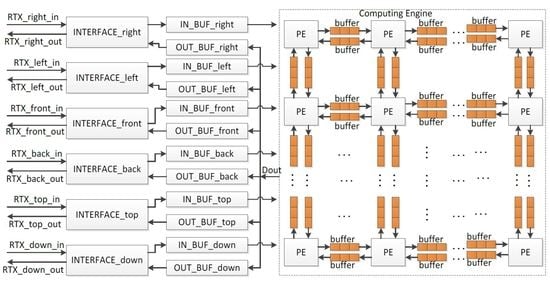
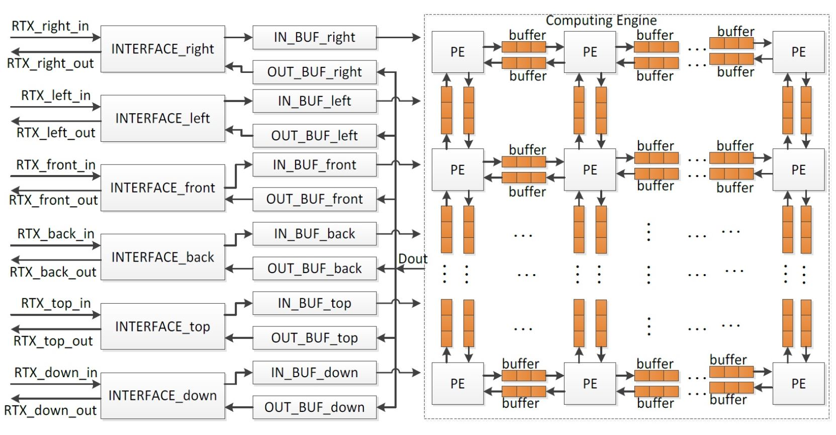
Since a sound space is divided into small grids, the simple architecture is to apply a computing unit at each grid to analyze the sound behavior. At a time step, computing units read data from their neighbors, carry out a computation, and output the calculation results to their neighbors. The temporary data are kept by computing units for further calculation. The whole system is fully parallel architecture, and the sample rate of the output sound is affected by the clock frequency of the computing units and the cycle count taken by the computing unit to complete computation in a time step. The computing units usually run at more than 100 MHz and complete computation in a time step less than 10 cycles. The rendering systems with the parallel architecture, therefore, achieve high sample rate in the output sound. However, the consumed hardware resources are increased exponentially as the number of grids is increased. The simulated area by a chip is hence small. To extend the simulated area, the rendering system with the time-sharing architecture was proposed [19], in which all data were stored in the block random access memories (RAMs) inside FPGA and sound pressures were calculated grid by grid through a computing unit. Although the simulated sound area by a single FPGA was enlarged by 37 times, the sample rate of the output sound was just 12.5 kHz, which would be further reduced as the number of grids was increased. To address these problems, a real-time sound rendering processor with the hybrid architecture was proposed in this research. The whole system is shown in Figure 1, and consists of the Computing Engine, in/out buffers, and the interfaces at six directions for data exchange when multiple chips are cascaded to perform sound rendering in a large sound space. The functions of components are shown as follows in detail.
- Computing Engine. The Computing Engine calculates the sound pressures of grids, and it is the core of the system. In the current solution, a sound space is divided into small sub-spaces, for example, a sound space with 8 × 8 × 8 grids can be divided into 8 small sub-spaces with each having 4 × 4 × 4 grids. A PE is used to analyze sound behavior in each small sub-space, and all PEs are cascaded to work in parallel to perform rendering in the whole sound space. The sound pressures of the grids on the boundaries between neighboring small sound spaces are written into the relevant buffers for further use by the neighbor PEs. Therefore, two buffers are required between two neighboring PEs. They are applied to keep the input data from and output data for the neighbor PE.
- INTERFACEs. The INTERFACEs provide the possibility for system scalability to extend the simulated sound area. From Equation (6), when multiple processors are cascaded, one chip exchanges data with neighbor chips in six directions, namely top, down, right, left, front, and back. Thus, a processor provides six interfaces for data communication.
- IN_BUFs and OUT_BUFs. The IN_BUFs and OUT_BUFs are utilized to store the sound pressures of grids on the boundaries between the neighboring small sound spaces when multiple processors are cascaded to perform rendering in a much larger sound space. The data from the neighbor processors are stored in the IN_BUFS and the data for the neighbor chips are kept by the OUT_BUFs.
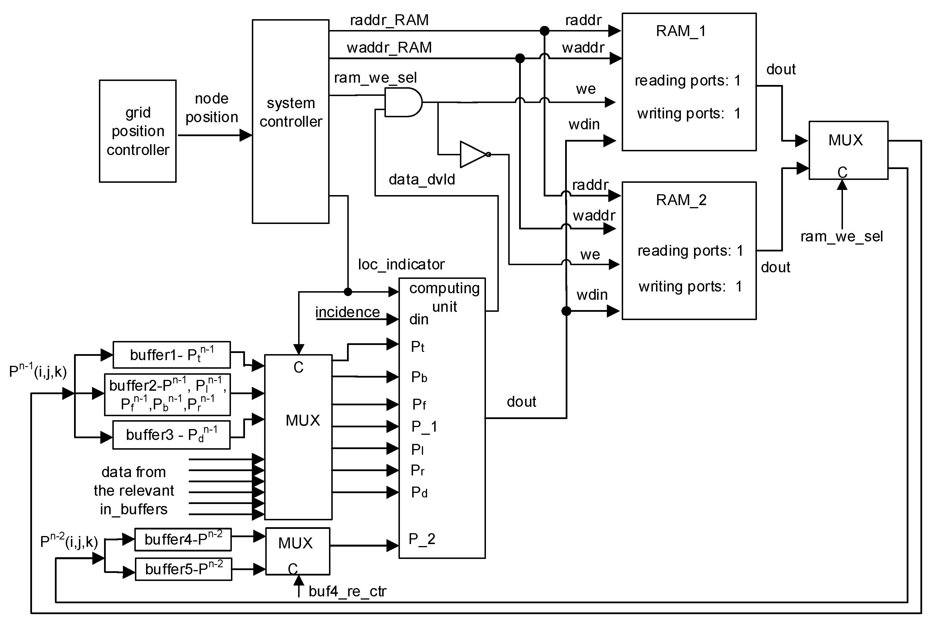
3.1. Processing Elements
The PE should be as simple as possible to reduce hardware resource consumption and improve system clock frequency. As shown in Figure 2, a PE consists of the computing unit, the grid position controller, system controller, five buffers, three multiplexers, and two block RAMs: RAM_1 and RAM_2. The PE is based on the time-sharing architecture [19] to extend the rendered area. At a time step, the computing unit reads data from the relevant buffers (buffer 1–5) or the IN_BUFs in accordance with the grid position, carries out computation, and writes the results to the RAM or the OUT_BUFs. After the calculation at a grid is completed, the computation is then shifted to the next grid until sound pressures of all grids are calculated. The modules in a PE are introduced as follows:
- Computing Unit. The computing unit calculates the sound pressure of a grid according to the input sound pressures at previous time steps, location indicators, and incident data. Based on Equation (13), a uniform computing unit was designed, which consists of a 7-input adder, a subtractor, two 32-bit fixed-point multipliers, and four multiplexers [19]. In Figure 3, the multipliers are for boundary grids while they are replaced by the right and left shifters for grids outside boundaries. The multiplicands are selected by the multiplexers according to the location indicator of a grid.
- Grid Position Controller. The grid position controller generates the grid position by using a counter, which is updated at every clock cycle.
- System Controller. The system controller maintains the computation flow and generates control signals, such as grid location flag (loc_indicator), read/write enable signal (we) of the RAMs, reading/writing addresses of the RAMs (raddr_RAM and waddr_RAM), and RAM selection signal (ram_we_sel).
- RAM_1 and RAM_2. The sound pressures of grids at previous one and two time steps, namely and , are stored in the RAM_1 and RAM_2. During computation, sound pressures at different time steps are stored in and read out from the RAM_1 and RAM_2 alternatively, and the calculation results at current time step are kept by the same RAM as that in which the sound pressures of grids at the previous two time steps are stored. For example, at a time step, and are stored in RAM_1 and RAM_2, respectively. Then, the calculation results at the current time step are written into the RAM_2. At the next time step, the reading and writing operations for the RAMs are switched; is read out from the RAM_1 while others are taken from the RAM_2. In addition, the calculation results are stored in the RAM_2. Such switching for RAM operations is repeated until all calculated time steps are over. The writing-enable signals of the RAMs are controlled by the signals ram_we_sel and data_dvld output by the system controller and the computing unit, respectively. When computations at a time step are finished, the signal ram_we_sel is reversed to invert the writing-enable signals of the RAMs. The size of RAMs is determined by the number of grids and data width. If data are 32-bit, and a sound space has N × M × L grids, each RAM is 4 NML bytes.
- Buffer 1–5. Data are read out from the RAMs and written in the five buffers in advance to reduce data access latency during calculation. The buffers are updated along with the computation. If data width is 32-bit, and a sound space has N × M × L grids, each buffer is 4 NM bytes in size.
- Multiplexers. Three multiplexers are used to select data for the computing unit. In the system, the input data of the computing unit may be from the local buffers within the same PE or the external input buffer, in which the data from the neighbor PE are stored.
3.2. INTERFACEs
The INTERFACEs are provided for system scalability. When multiple processors are cascaded, control instructions and temporary data during computation need to exchange with the neighbor processors. Through the INTERFACEs, multiple processors are easily connected to each other to extend the rendered sound space. As shown in Figure 4, the INTERFACE consists of receiver, decoder, and transmitter. And they are introduced more detail as follows.
- Receiver. The receiver receives serial data from the neighbor processors, checks the data type (data or control instructions), and stores data to the first in first out (FIFO) buffer or buffer according to the data type. The receiver is composed of a data type detector (RX_FHD) and a state machine (RX_STATE) to control the receiving flow. As shown in Figure 5, the system firstly detects the 8-bit type flag, which is AB and 54 in hexadecimal for pure data and the control instructions, respectively. After the type flag is received, system then receives the data length, which is 8-bit and denotes the data length in byte. Finally, data are received and stored in the RX_FIFO for the control instructions or IN_BUF for the pure data.
- Decoder. The DECODER decodes and executes the control instructions. Eleven control instructions are defined for system configuration and data communication. Furthermore, an automatic instruction forwarding mechanism is provided to forward the control instructions to other processors when multiple processors are cascaded.
- Transmitter. The transmitter (TX_STATE) transmits the control instructions or pure data to the neighbor processors. Data are transmitted in the manner of data frame, which consists of type flag, data length, chip ID, and the relevant pure data or instructions. Before data transmission, the bus is checked. If it is free, transmission is started; otherwise, the system waits for some clock cycles and checks again until the bus is free. Three types of data are transmitted, which are pure data, forwarded instructions, and the acknowledgement instruction. To transmit the pure data or the forwarded instructions, the data valid instruction is firstly sent out. Then, the system waits for the acknowledgment signal from the receiver. After the signal is received, the related data frame is transmitted serially. When the system receives the data valid instruction from the neighbor processors, it responds the data communication request by sending back the acknowledgement instruction. The whole procedure is shown in Figure 6 and is controlled by a state machine.
4. Performance Estimation
To verify and estimate system performance, the register transfer level (RTL) model and cycle-accurate simulator of the processor were developed using VHDL and C programming language. Furthermore, the prototype machine was investigated and implemented using a processor-based FPGA machine TD-SPP3000 from Tokyo Electron Device Ltd., and sound propagation in a small shoe-box type room was examined. In the defined room, both length and width were 1.28 m, and height was 0.64 m; the cube grid size was 4 × 10⁻² m; the reflection factor of the boundaries was 0.95; and the incident and observation points were at the middle of the room. Therefore, the small room was discretized into a mesh with 32 × 32 × 16 grids. The hardware development environment was a 64-bit Windows 7 platform with FPGA tools Xilinx ISE 14.3 and ModelSim SE 10.1d. For comparison, the counterpart system was also developed by C++ programming language, and executed on a personal computer (PC) with 32 GB RAM and an Intel i7-6800K six-core processor running at 3.4 GHz. The software environment of the PC was 64-bit CentOS 7.0 with gcc 4.9.4. The reference C++ codes were compiled and optimized by using the command g++ with the option -O3, mcmodel = large, and -fopenmp to use all six cores in the PC. Data were 32-bit fixed-point in the prototype machine while they were integer in the software simulations.
The prototype machine consisted of two FPGA boards, and each board contained two XC5VLX330T-FF1738 FPGA chips from Xilinx. A high-speed A/D board (ADS5474) was attached to the FPGA1 on the board 1 to sample the incident signals. Then, the sampled data were processed by the rendering processor implemented by the FPGA1 on the board 1. The sound pressures at the observation point were transferred to the D/A board (DAC5682Z) on the board 2 through the advanced telecommunication computing architecture (ATCA) bus and output to drive the speakers directly. The rendering processor and the A/D and D/A boards all ran at 200 MHz. In the rendering processor, each PE processed the sound rendering in a sound space with 4 × 4 × 4 grids, and all PEs worked in parallel to carry out rendering at the whole sound space. Thus, computation at each time step took 64 cycles, and each cycle was 5 (1/(200 × 106)) ns.
4.1. Performance of the Prototype Machine
4.1.1. Rendering Time
Table 2 shows the rendering time taken by the prototype machine and the software simulation on the PC using six cores to render a three-minute Beethoven wave sound in the defined small shoe-box type room.
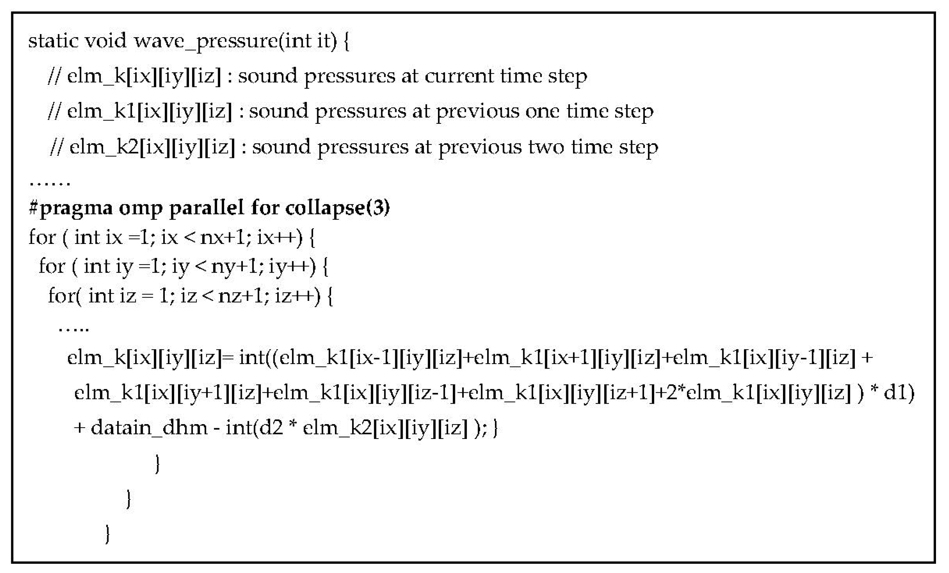
As shown in Table 2, the rendering task consumes about 12.70 min (762.25/60) in the offline software simulation on the PC, while it is handled at run-time on the prototype machine. Figure 7 shows the computation flow in the software simulation. In the software simulation, all the incident data were firstly read from an incident wave file and stored in a buffer. At each time step, an incident datum is read and sound pressures of all grids are calculated, the sound pressure of the observation point is updated, and the sound pressures of grids at current time step and previous time steps are swapped. This procedure is iterated until all time steps are completed. Since the swap operation must be operated after the sound pressures of all grids are obtained, the outer loop cannot be parallelized while the computation and data swap modules (shown in yellow in Figure 7) are parallelized by using OpenMP. Figure 8 and Figure 9 present parts of the source code of the computation and data swap modules in which the directives of OpenMP are shown by the bold words. The three loops in the computation and data swap modules are parallelized through being collapsed into one large iteration space and then divided according to the valid threads. Figure 10 depicts the computation time in the case of different numbers of cores being applied in the software simulation. As the number of cores is increased, the computation time is decreased due to system parallelization using OpenMP. When six cores are all used for computation, the computation time is 762.25 s, which is about 18% of the computation time when a single core is applied in calculation.
In the prototype machine, the incident wave sound is played by a media player and sampled by the A/D board as incidences at each time step; then rendering is carried out and, finally, the rendered results are output through the D/A board to drive the speakers directly. Therefore, the rendering is carried out at run-time, and the rendered results at each time step are output by the D/A board directly. When the input incident wave is finished, the rendering is also completed after the operations when the final time step is over. Consequently, the whole rendering procedure lasts the same period as the length of the incident sound plus the time taken by the computation at the final time step, namely 3 min plus 64 cycles (3 s + 320 ns). In the computer-based software simulation, data are stored in the external main memory, the rendered results are temporarily kept by an array at each time step, and finally written to a wave file. During computation, main memory is accessed frequently to read data out or write data back, which is time-consuming. In contrast, data are stored in the on-chip memory (block RAMs inside FPGA) in the prototype machine, and they are accessed in one or two cycles. Furthermore, five buffers are applied to read data out in advance to reduce data access overhead in the PE. On the other hand, the rendering processor is the hybrid architecture, and many PEs work in parallel to speed up computation. Because each PE is applied to analyze sound behavior at a sound space with 4 × 4 × 4 grids, the prototype machine contains 256 ((32 × 32 × 16)/(4 × 4 × 4)) PEs to work in parallel, and speeds up computation by 256 times in comparison with the rendering system with the time-sharing architecture, in which only one PE is applied to carry out rendering.
The rendering processor is designed through pipelining, and the rendered results are consecutively output by the D/A board after a one-cycle delay. To investigate the effect of such a small delay on the output and system stability, a pulse with amplitude of 16,384 Pa was launched into the prototype system, and the impulse response of the defined shoe-box room is presented in Figure 11. As shown in Figure 11, the output was just delayed one-cycle, and the system became stable after 400 time steps. Thus, the small delay almost has no effect on the system.
4.1.2. Sample Rate of the Output Sound
Although the prototype machine carries out sound rendering at run-time, the output sound quality is worse than that output by the offline computer-based software simulation. In the software simulation, incident data are read from a sound wave file directly at each time step, and the rendering results are written into another sound wave file after the computation is finished. The output sound wave, therefore, has same sample rate and bitrate as the incidence. However, in the prototype machine, the sample rate of the output sound is calculated through Equation (14).
is the system clock frequency, and denotes the number of grids processed by a PE. In the current prototype machine, since each PE performs sound rendering in a sound space with 4 × 4 × 4 grids, and the system clock frequency is 200 MHz, the sample rate of the output sound is about 3.125 MHz (200 MHz/64). Compared with the rendering system with the time-sharing architecture, in which the sample rate of the output sound is about 12.5 kHz [19], the prototype achieves about 256 times gain in sample rate of the output sound. In the rendering system with the time-sharing architecture, only a computing unit is applied to calculate the sound pressure grid by grid. Hence, as the number of grids is increased, the computation time at a time step will become longer, which results in a low sample rate of the output sound. However, the proposed rendering processor is the hybrid architecture, in which the top level is the parallel architecture, and the PE is based on the time-sharing architecture. Therefore, the computation is speeded up, and high sample rate is obtained in the output sound.
On the other hand, the incidence is input through an A/D converter and the rendered results are output through a D/A converter in the prototype machine. Because the A/D converter is 14-bit, each incident datum is 14-bit, but it is 16-bit in the software simulation. This long data width of the incidence results in high accuracy in computation in the software simulation. Furthermore, each PE performs sound rendering in a sound space with 4 × 4 × 4 grids, if the computation at a grid is completed at one cycle through a pipelining technique, calculation at a time step takes 64 cycles. In other words, the incidence will be input in the system every 64 cycles from the A/D converter. This may result in the information loss in the incident wave sound, and reduce the computation accuracy. Another factor to affect the output sound quality comes from the electronic noise of the A/D and D/A boards. When the prototype machine has no input at the A/D converter, the electronic noise can be heard at the output of the D/A converter. Compared with professional audio devices, current A/D and D/A converters provides worse performance in suppressing electronic noise.
4.1.3. Throughput
The throughput denotes the number of grids updated per second, and is calculated by Equation (15).
Here, is the number of grids, is the number of time steps, and is the calculation time. In the software simulation, the incident sound wave has 9,022,848 data, and each datum will be input into the system as an incidence. Nevertheless, the time steps are 9,022,848. From Table 2 and Figure 10, when six processor cores are applied, the throughput in the software simulation is about 194 (32 × 32 × 16/(762.25/9,022,848)) M grids/s. In the prototype machine, the computations at each time step are completed in 64 (4 × 4 × 4) cycles. Thus, the throughput is about 51.2 (32 × 32 × 16/(64 × 1/0.2) G grids/s. Even if the clock frequency of the prototype is much lower than the PC, the throughput is much higher. Compared with the PC-based simulation, the prototype machine achieves about 263.9 times gain in throughput.
4.2. System Implementation by ASIC
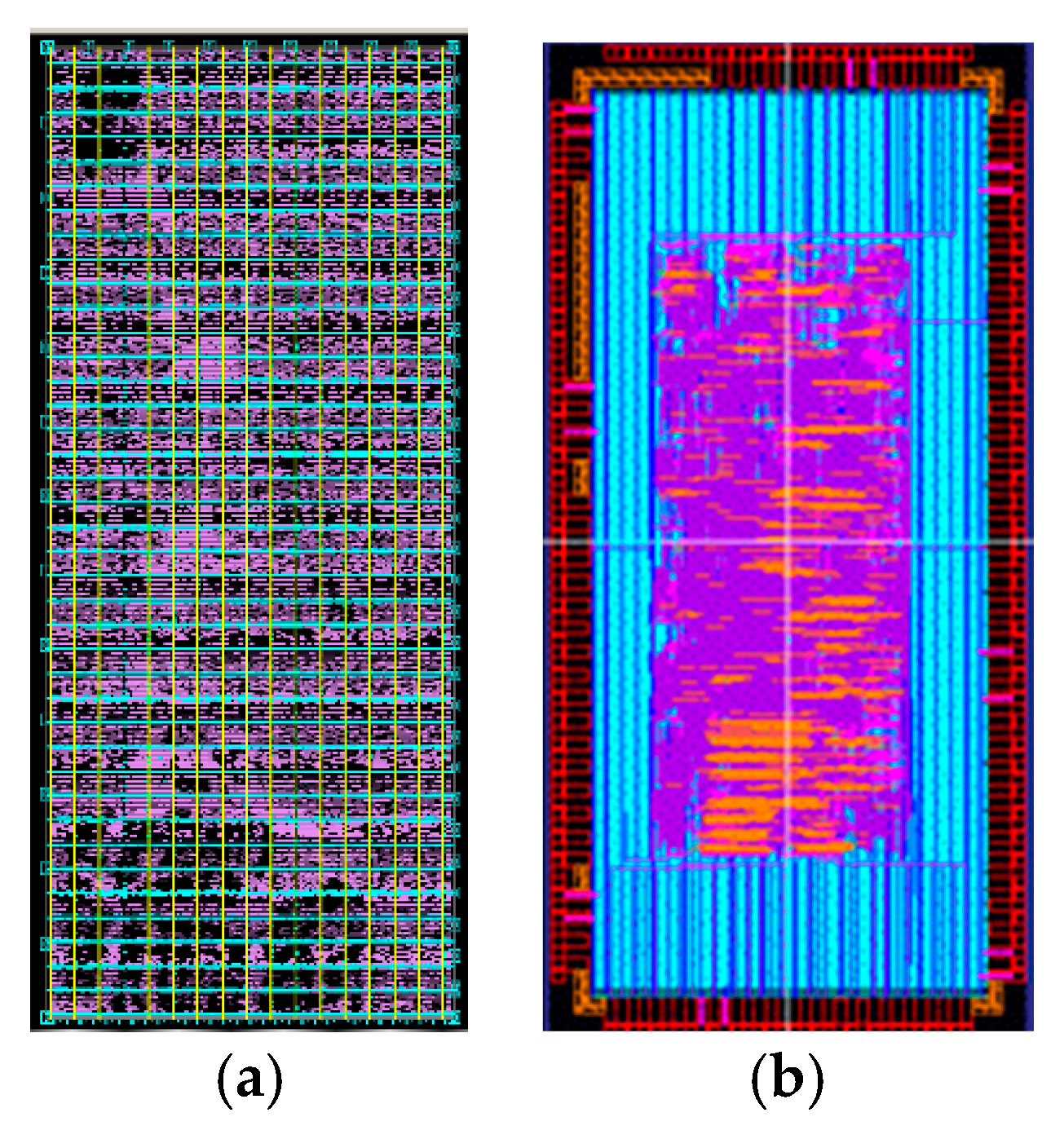
A trial processor with a PE and interfaces was developed and taped out by using the 0.18 µm processing technology from the ROHM semiconductor Co. Ltd. through the fabrication service provided by the VLSI design and education center at University of Tokyo. When the PE is utilized to process 4 × 4 × 4 grids, the layouts of the processor and the whole chip are shown in Figure 12a,b, respectively. The chip is 2.5 mm × 5.0 mm in size, and contains 89 pins [26]. The whole system consumes 238,515 gates, and the power consumption is about 143.8 mW. The system clock frequency is 200 MHz.
5. Conclusions
Real-time sound rendering is computation-intensive. The output sound quality and system scalability are two concerning issues in the design of a real-time sound rendering system by hardware. In this research, a real-time sound rendering processor with the hybrid architecture was investigated and implemented to speed up computation and improve the sample rate of the output sound. While rendering sound in a small shoe-box room with dimensions of 1.28 m × 1.28 m × 0.64 m, the proposed processor performs sound rendering at real-time, while the offline computer-based software simulation takes about 12.70 min. Compared with the FPGA-based sound rendering system with the time-sharing architecture, our processor achieves 256 times increase in computation speed and improvement in the sample rate of the output sound.
Furthermore, owing to the limited hardware resources inside a single chip, multiple chips are usually required to carry out rendering for a large sound space. To make the system easily extendable, interfaces were provided in the proposed sound rendering processor for system scalability. Through the interfaces, multiple processors are easily connected to each other to extend the rendered sound space. Although the current interface achieves good performance in data transmission and system scalability, the data transmission speed is limited due to data width. In future work, the serial advanced technology attachment (SATA) interface will be investigated and applied in the processor to enhance the data transfer speed.
Acknowledgment
This work was supported in part by the Strategic Information and Communications R&D Promotion Programme (SCOPE), Ministry of Internal Affairs and Communications. Thanks for Professor Imamura Toshiyuki’s valuable discussion on the system parallelization by using OpenMP.
Author Contributions
Tan Yiyu and Yasushi Inoguchi specified the system architecture and designed the system. Tan Yiyu and Takao Tsuchiya discussed and derived the algorithm, Makoto Otani, Yukio Iwaya, Takao Tsuchiya, and Yasushi Inoguchi conceived the system solution and helped debug prototype system. Tan Yiyu and Yasushi Inoguchi wrote and revised the paper.
Conflicts of Interest
The authors declare no conflict of interest.
References
- Botteldooren, D. Acoustical finite-difference time-domain simulation in a quasi-Cartesian grid. J. Acoust. Soc. Am. 1994, 95, 2313–2319. [Google Scholar] [CrossRef]
- Botteldooren, D. Finite-difference time-domain simulation of low-frequency room acoustic problems. J. Acoust. Soc. Am. 1995, 98, 3302–3308. [Google Scholar] [CrossRef]
- Chiba, O.; Kashiwa, T.; Shimoda, H.; Kagami, S.; Fukai, I. Analysis of sound fields in three dimensional space by the time-dependent finite-difference method based on the leap frog algorithm. J. Acoust. Soc. Jpn. 1993, 49, 551–562. [Google Scholar]
- Savioja, L.; Valimaki, V. Interpolated rectangular 3-D digital waveguide mesh algorithms with frequency warping. IEEE Trans. Speech Audio Process. 2003, 11, 783–790. [Google Scholar] [CrossRef]
- Campos, G.R.; Howard, D.M. On the computational efficiency of different waveguide mesh topologies for room acoustic simulation. IEEE Trans. Speech Audio Process. 2005, 13, 1063–1072. [Google Scholar] [CrossRef]
- Murphy, D.T.; Kelloniemi, A.; Mullen, J.; Shelley, S. Acoustic modeling using the digital waveguide mesh. IEEE Signal Process. Mag. 2007, 24, 55–66. [Google Scholar] [CrossRef] [Green Version]
- Kowalczyk, K.; van Walstijn, M. Room acoustics simulation using 3-D compact explicit FDTD schemes. IEEE Trans. Audio Speech Lang. Process. 2011, 19, 34–46. [Google Scholar] [CrossRef] [Green Version]
- Van Mourik, J.; Murphy, D. Explicit higher-order FDTD schemes for 3D room acoustic simulation. IEEE/ACM Trans. Audio Speech Lang. Process. 2014, 22, 2003–2011. [Google Scholar] [CrossRef]
- Hamilton, B.; Bilbao, S. Fourth-order and optimised finite difference schemes for the 2-D wave equation. In Proceedings of the 16th Conference on Digital Audio Effects (DAFx-13), Maynooth, Ireland, 2–6 September 2013. [Google Scholar]
- Hamilton, B.; Bilbao, S.; Webb, C.J. Revisiting implicit finite difference schemes for 3D room acoustics simulations on GPU. In Proceedings of the International Conference on Digital Audio Effects (DAFx-14), Erlangen, Germany, 1–5 September 2014; pp. 41–48. [Google Scholar]
- Brian, H.; Stefan, B. FDTD methods for 3-D room acoustics simulation with high-order accuracy in space and time. IEEE/ACM Trans. Audio Speech Lang. Process. 2017, 25, 2112–2124. [Google Scholar]
- Valimäki, V.; Parker, J.D.; Savioja, L.; Smith, J.O.; Abel, J.S. Fifty years of artificial reverberation. IEEE Trans. Audio Speech Lang. Process. 2012, 20, 1421–1448. [Google Scholar] [CrossRef]
- Ishii, T.; Tsuchiya, T.; Okubo, K. Three-dimensional sound field analysis using compact explicit-finite difference time domain method with Graphics Processing Unit Cluster System. Jpn. J. Appl. Phys. 2013, 52, 07HC11. [Google Scholar] [CrossRef]
- Tsuchiya, T. Three-dimensional sound field rendering with digital boundary condition using graphics processing unit. Jpn. J. Appl. Phys. 2010, 49, 07HC10. [Google Scholar] [CrossRef]
- Savioja, L. Real-time 3D finite difference time domain simulation of low and mid-frequency room acoustics. In Proceedings of the International Conference on DAFx, Graz, Austria, 6–10 September 2010; pp. 77–84. [Google Scholar]
- Tanaka, M.; Tsuchiya, T.; Okubo, K. Two-dimensional numerical analysis of nonlinear sound wave propagation using constrained interpolation profile method including nonlinear effect in advection equation. Jpn. J. Appl. Phys. 2011, 50, 07HE17. [Google Scholar] [CrossRef]
- Tan, Y.Y.; Inoguchi, Y.; Sugawara, E.; Otani, M.; Iwaya, Y.; Sato, Y.; Matsuoka, H.; Tsuchiya, T. A real-time sound field renderer based on digital Huygens’ model. J. Sound Vib. 2011, 330, 4302–4312. [Google Scholar]
- Tan, Y.Y.; Inoguchi, Y.; Sato, Y.; Otani, M.; Iwaya, Y.; Matsuoka, H.; Tsuchiya, T. A hardware-oriented finite-difference time-domain algorithm for sound field rendering. Jpn. J. Appl. Phys. 2013, 52, 07HC03. [Google Scholar]
- Tan, Y.Y.; Inoguchi, Y.; Sato, Y.; Otani, M.; Iwaya, Y.; Matsuoka, H.; Tsuchiya, T. A real-time sound rendering system based on the finite-difference time-domain algorithm. Jpn. J. Appl. Phys. 2014, 53, 07KC14. [Google Scholar]
- Tan, Y.Y.; Inoguchi, Y.; Sato, Y.; Otani, M.; Iwaya, Y.; Matsuoka, H.; Tsuchiya, T. Analysis of sound field distribution for room acoustics: from the point of view of hardware implementation. In Proceedings of the International Conference on DAFx, York, UK, 17–21 September 2012; pp. 93–96. [Google Scholar]
- Tan, Y.Y.; Inoguchi, Y.; Sugawara, E.; Sato, Y.; Otani, M.; Iwaya, Y.; Matsuoka, H.; Tsuchiya, T. A FPGA implementation of the two-dimensional digital huygens model. In Proceedings of the International Conference on Field Programmable Technology (FPT), Beijing, China, 8–10 December 2010; pp. 304–307. [Google Scholar]
- Inoguchi, Y.; Tan, Y.Y.; Sato, Y.; Otani, M.; Iwaya, Y.; Matsuoka, H.; Tsuchiya, T. DHM and FDTD based hardware sound field simulation acceleration. In Proceedings of the International Conference on DAFx, Paris, France, 19–23 September 2011; pp. 69–72. [Google Scholar]
- Kuttruff, H. Room Acoustics; Taylor & Francis: New York, NY, USA, 2009. [Google Scholar]
- Maxwell, J.C. A Treatise on Electricity and Magnetism, 3rd ed.; Clarendon: Oxford, UK, 1892; Volume 2, pp. 68–73. [Google Scholar]
- Kowalczyk, K.; Walstijn, M.V. Formulation of locally reacting surfaces in FDTD/K-DWM modelling of acoustic spaces. Acta Acust. United Acust. 2008, 94, 891–906. [Google Scholar] [CrossRef]
- Yiyu, T.; Inoguchi, Y.; Otani, M.; Iwaya, Y.; Tsuchiya, T. Design of a Real-time Sound Field Rendering Processor. In Proceedings of the RISP International Workshop on Nonlinear Circuits, Communications and Signal Processing, Honolulu, HI, USA, 6–9 March 2016; pp. 173–176. [Google Scholar]
Figure 1.
System diagram. Processing element (PE), receiving/transmission (RTX).
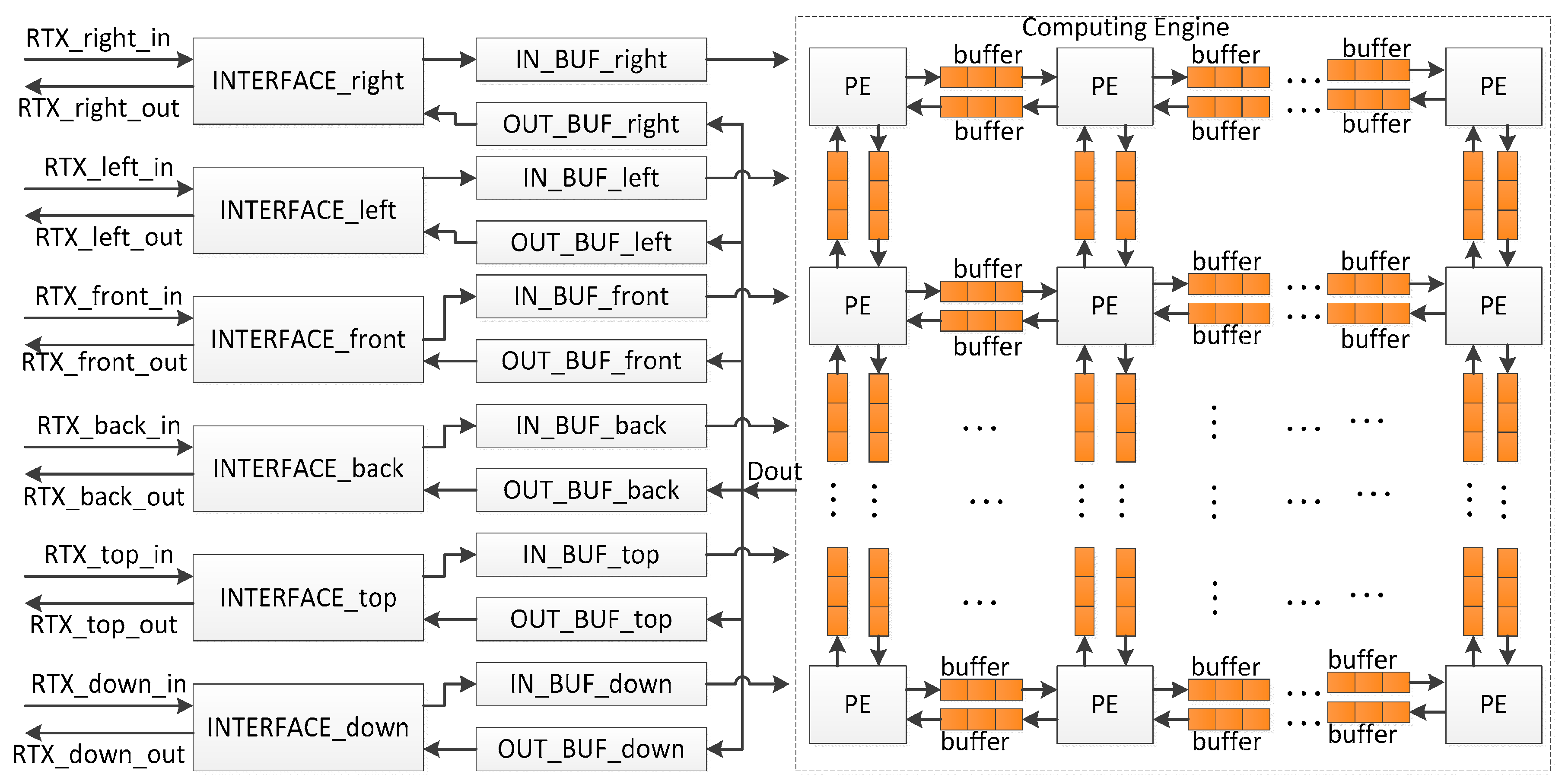
Figure 2.
System diagram of the PE.

Figure 3.
Computing unit.
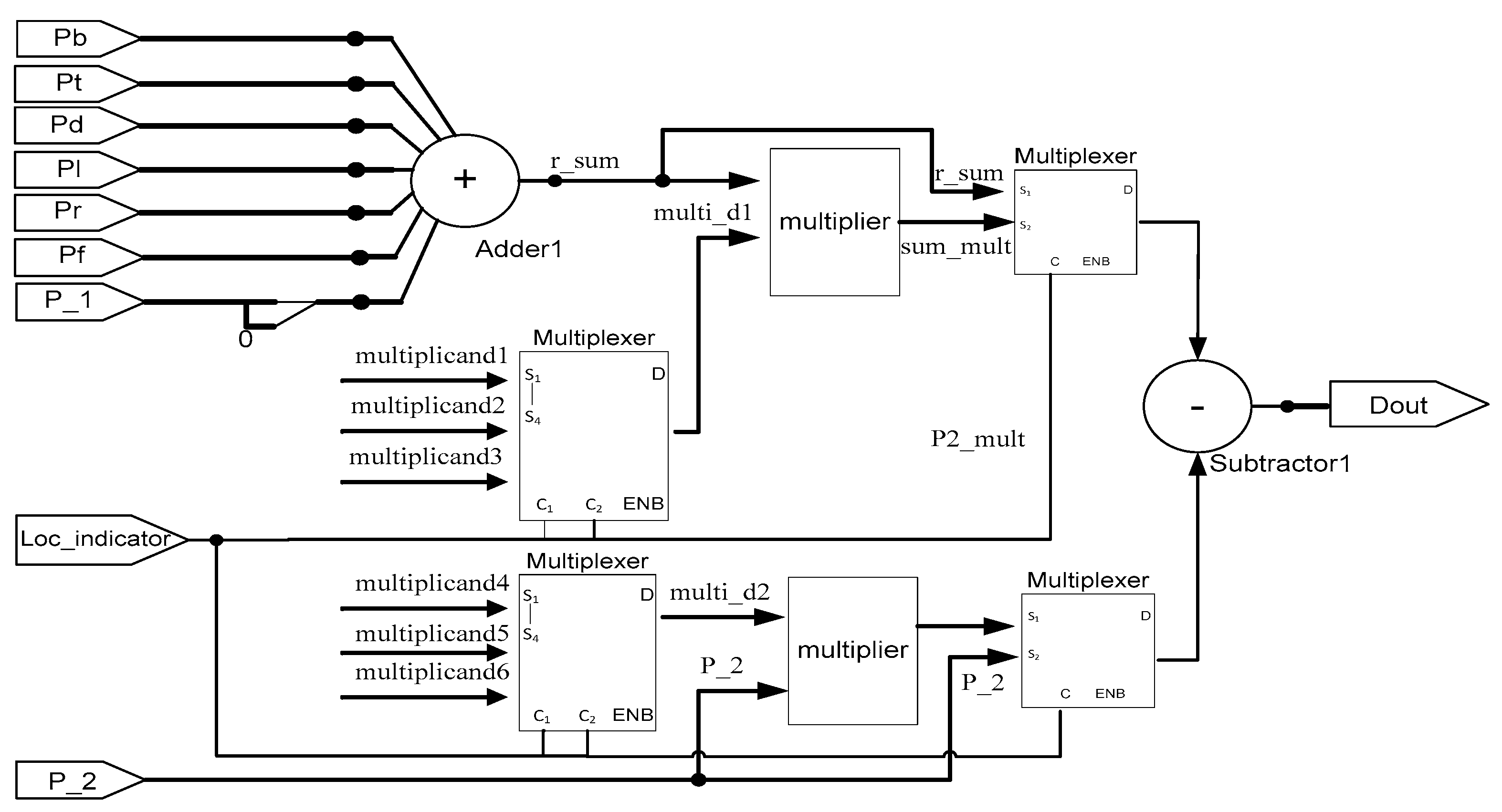
Figure 4.
Diagram of the INTERFACE.
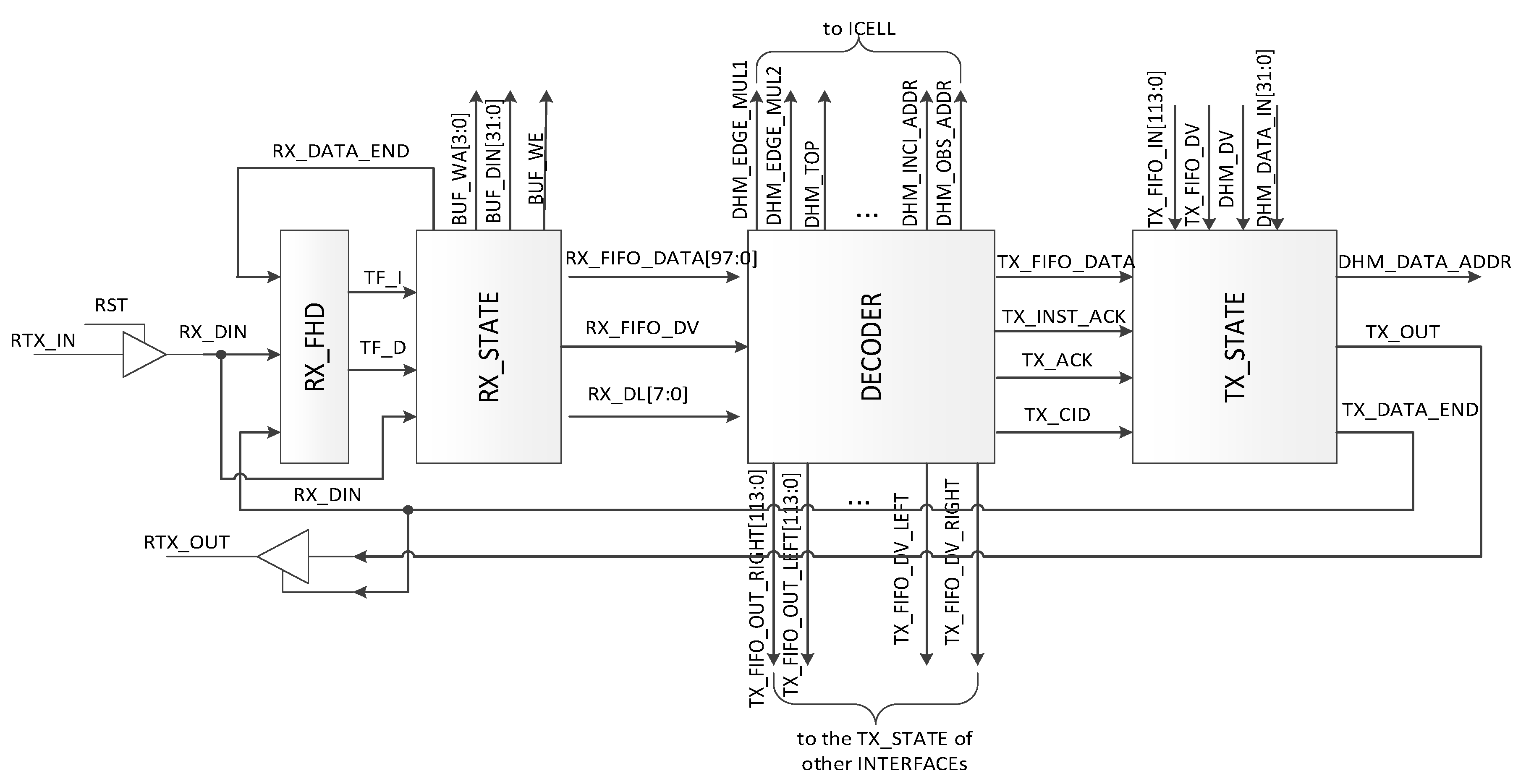
Figure 5.
Data receiving.
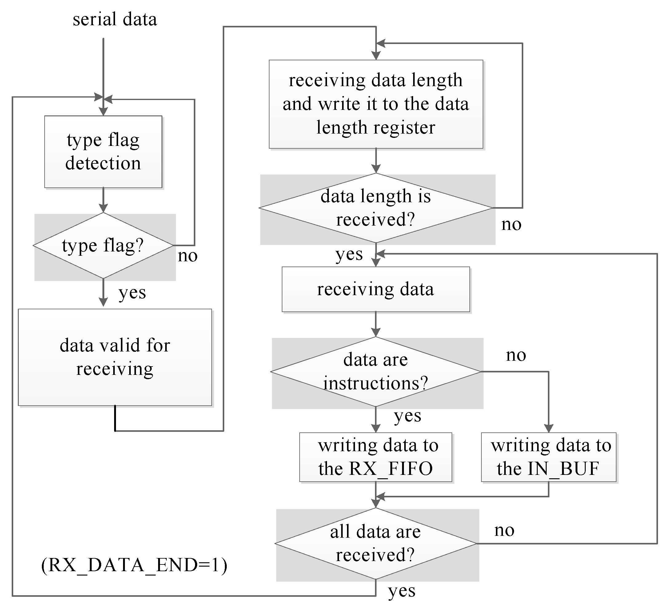
Figure 6.
Data transmission.
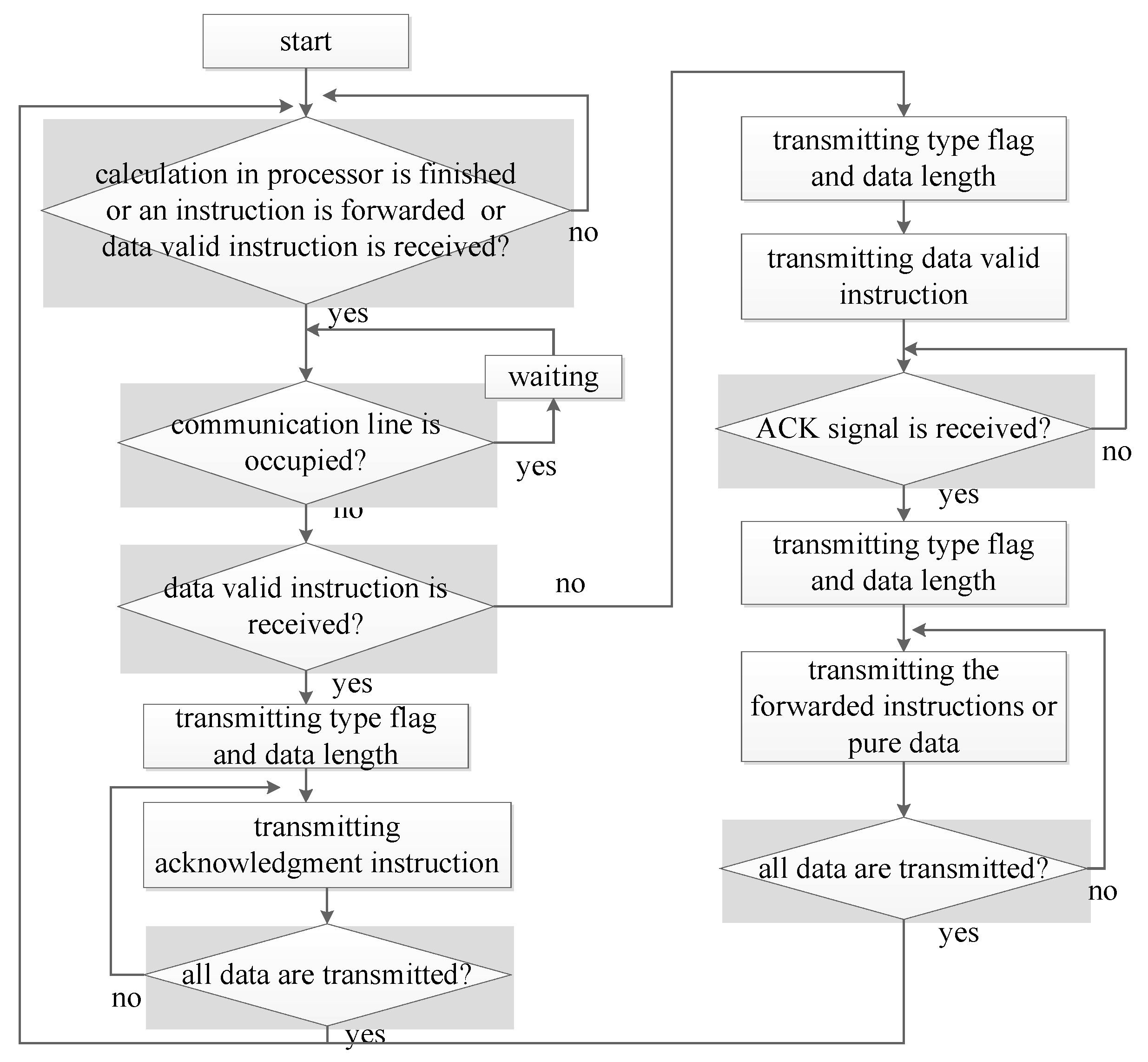
Figure 7.
Computation flow of the software simulation.
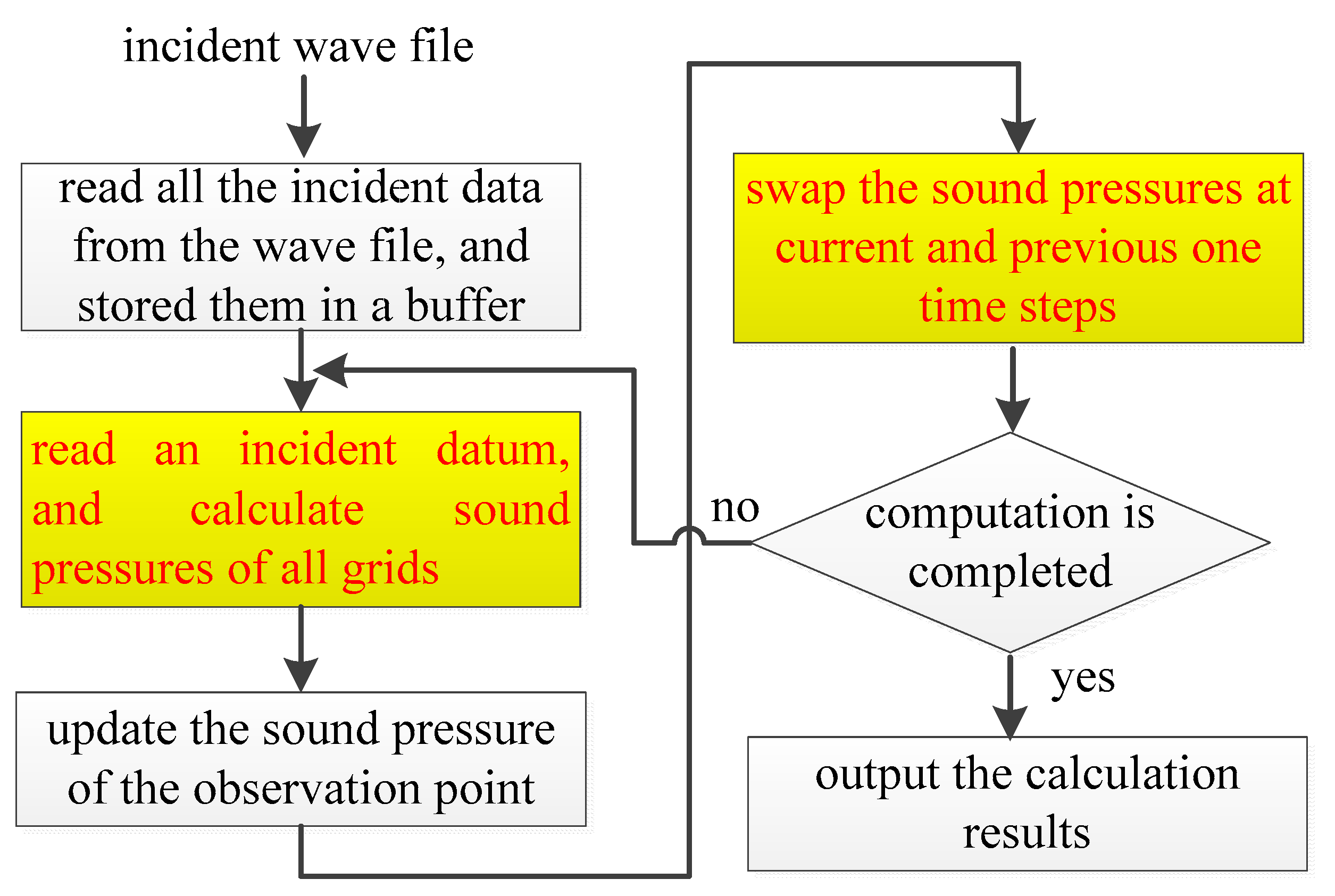
Figure 8.
Snapshot of the computation module.

Figure 9.
Snapshot of the data swap module.
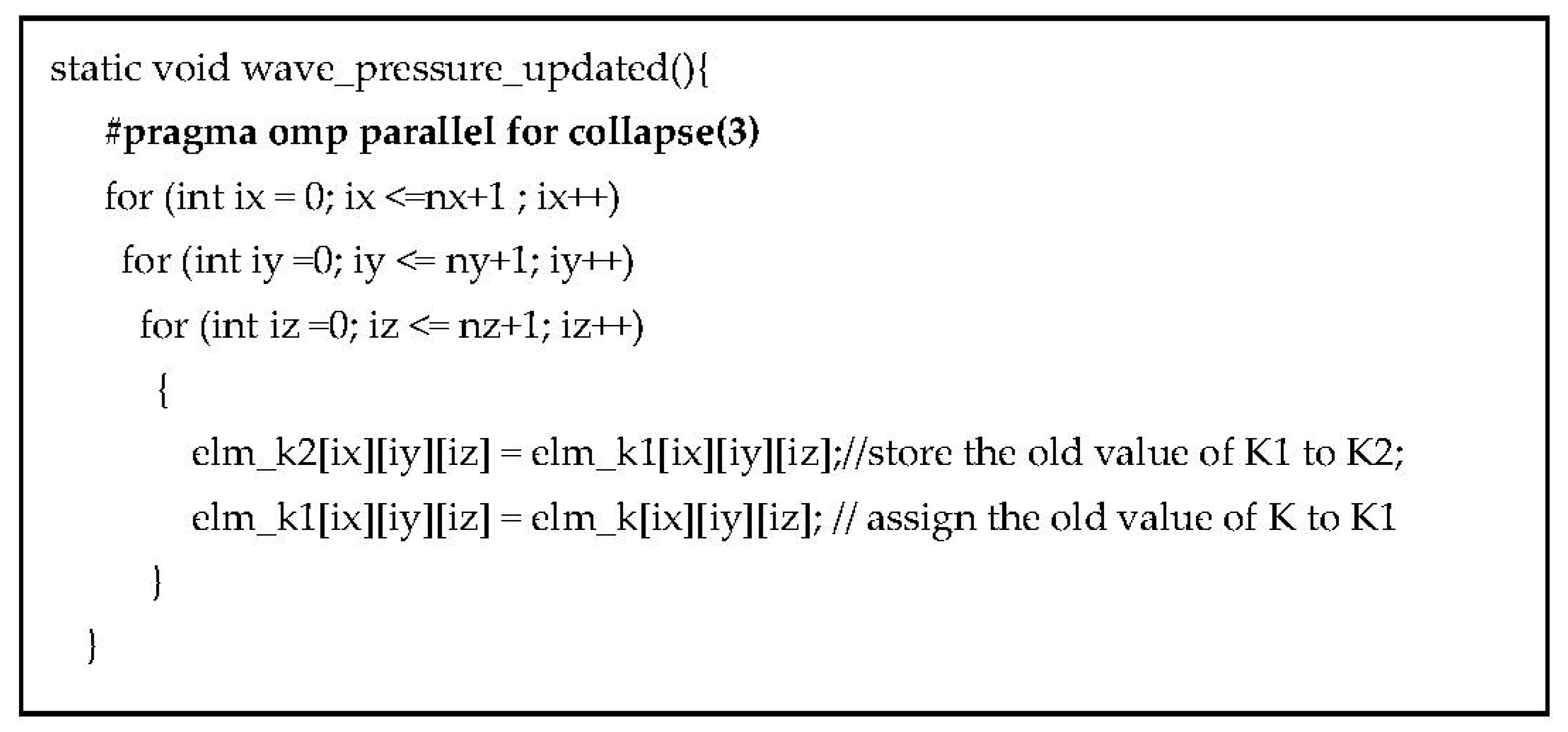
Figure 10.
Computation time by using the OpenMP in software simulation.
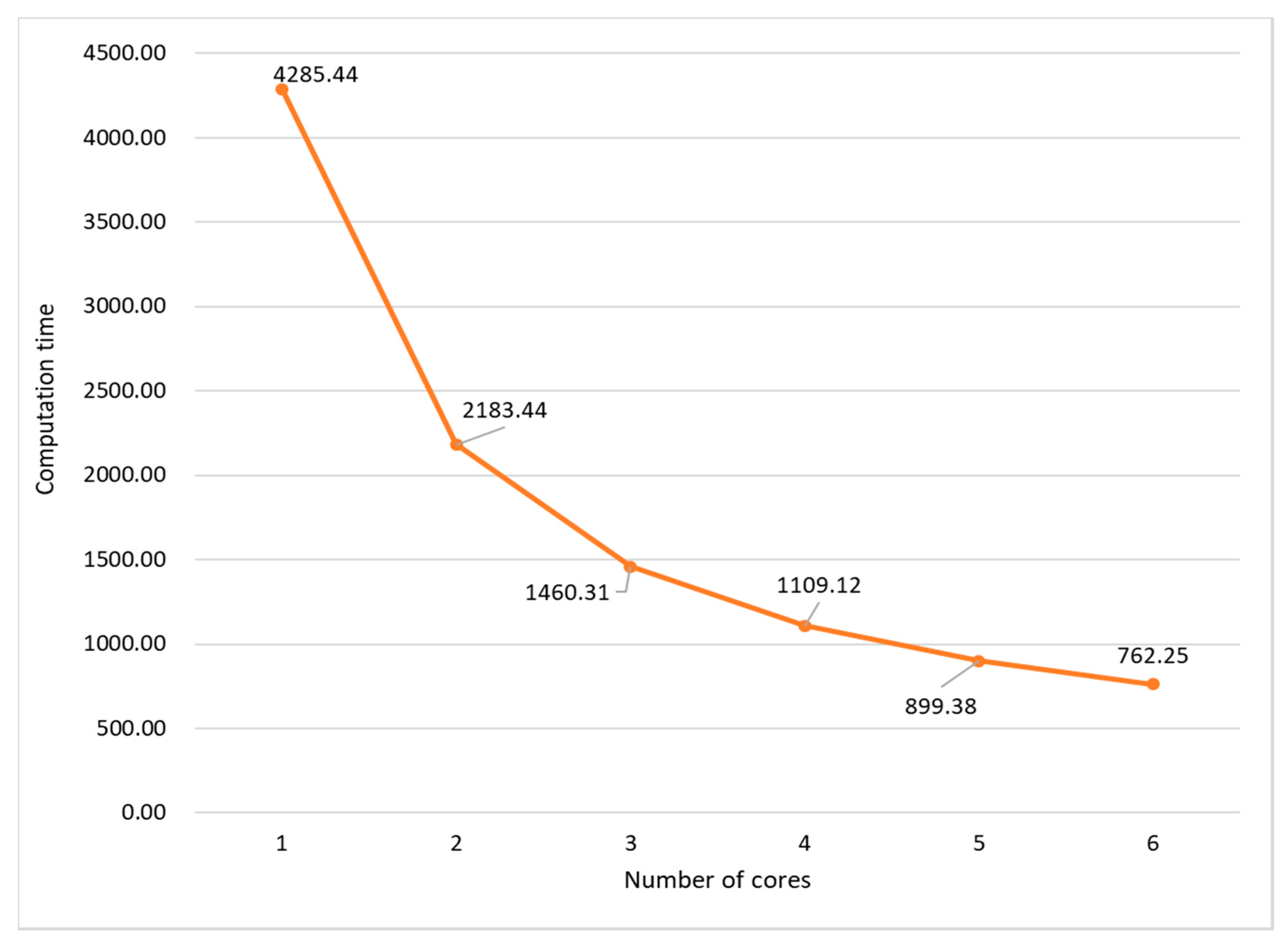
Figure 11.
Impulse response of the defined room.
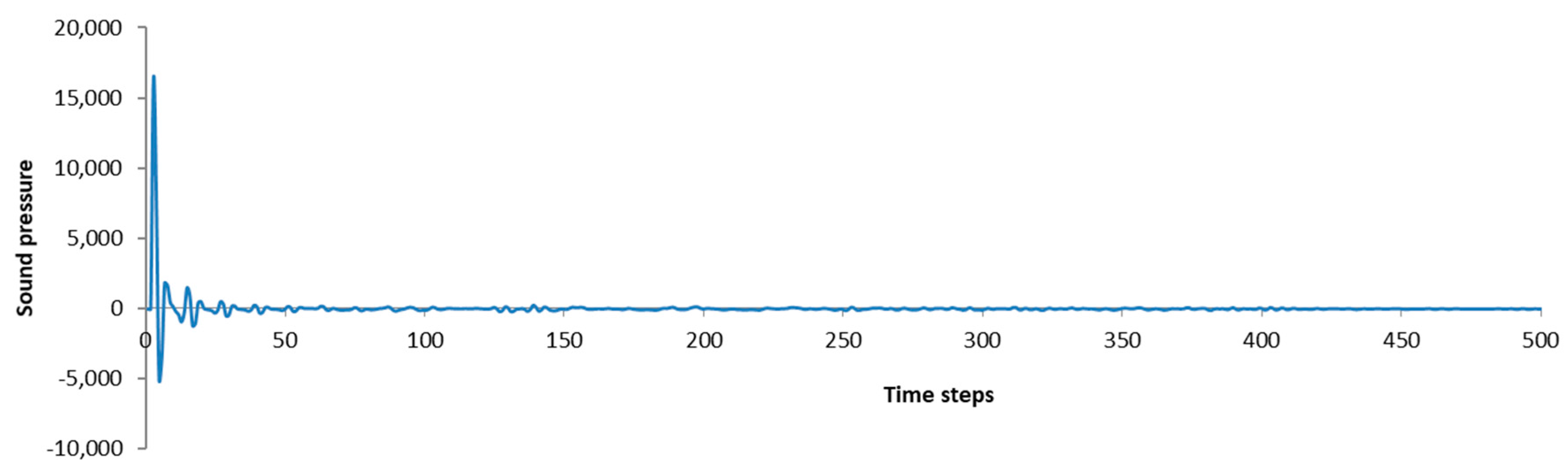
Figure 12.
(a) Layout of the processor (b) Layout of the chip.

Table 1.
Parameters.
| Grid Position | D1 | D2 |
|---|---|---|
| General | ||
| Interior | ||
| Edge | ||
| Corner |
Table 2.
Rendering time (s).
| Grid | Prototype | PC |
|---|---|---|
| 32 × 32 × 16 | run-time | 762.25 |
PC: personal computer.
© 2017 by the authors. Licensee MDPI, Basel, Switzerland. This article is an open access article distributed under the terms and conditions of the Creative Commons Attribution (CC BY) license (http://creativecommons.org/licenses/by/4.0/).
Share and Cite
MDPI and ACS Style
Yiyu, T.; Inoguchi, Y.; Otani, M.; Iwaya, Y.; Tsuchiya, T. A Real-Time Sound Field Rendering Processor. Appl. Sci. 2018, 8, 35. https://doi.org/10.3390/app8010035
AMA Style
Yiyu T, Inoguchi Y, Otani M, Iwaya Y, Tsuchiya T. A Real-Time Sound Field Rendering Processor. Applied Sciences. 2018; 8(1):35. https://doi.org/10.3390/app8010035
Chicago/Turabian StyleYiyu, Tan, Yasushi Inoguchi, Makoto Otani, Yukio Iwaya, and Takao Tsuchiya. 2018. "A Real-Time Sound Field Rendering Processor" Applied Sciences 8, no. 1: 35. https://doi.org/10.3390/app8010035
Note that from the first issue of 2016, this journal uses article numbers instead of page numbers. See further details here.