A Novel Approach for the Estimation of Doubly Spread Acoustic Channels Based on Wavelet Transform

1
School of Information Science and Engineering, Southeast University, Nanjing 210096, China
2
School of Electronic and Information Engineering, Qingdao University, Qingdao 266071, China
3
School of Automation and Electrical Engineering, Qingdao University, Qingdao 266071, China
*
Authors to whom correspondence should be addressed.
Appl. Sci. 2018, 8(1), 38; https://doi.org/10.3390/app8010038
Submission received: 29 October 2017
/
Revised: 20 December 2017
/
Accepted: 20 December 2017
/
Published: 1 January 2018
(This article belongs to the Special Issue Underwater Acoustics, Communications and Information Processing)
Abstract
:In this paper, the estimation of doubly spread underwater acoustic (UWA) channels is investigated. The UWA channels are characterized by severe delay spread and significant Doppler effects, and can be well modeled as a multi-scale multi-lag (MSML) channel. Furthermore, exploiting the sparsity of UWA channels, MSML channel estimation can be transformed into the estimation of parameter sets (amplitude, Doppler scale factor, time delay). Based on this, the orthogonal matching pursuit (OMP) algorithm has been widely used. However, the estimation accuracy of OMP depends on the size of the dictionary, which is related with both delay spread and Doppler spread. Thus it requires high computational complexity. This paper proposes a new method, called wavelet transform (WT) based algorithm, for the UWA channel estimation. Different from OMP algorithm which needs to search in both time domain and Doppler domain, WT-based algorithm only needs to search in time domain by using the Doppler invariant characteristic of hyperbolic frequency modulation (HFM) signal. The performance of the proposed algorithm is evaluated by computer simulations based on BELLHOP. The simulation results show that WT-based algorithm performs slightly better than OMP algorithm in low signal to noise ratio (SNR) while can greatly reduce computational complexity.
1. Introduction
Underwater acoustic (UWA) channels pose grand challenges for reliable high data-rate communications, due to significant Doppler effects and severe delay spread [1,2,3]. In underwater communications, acoustic waves propagate at 1500 m/s, much lower than the speed of electromagnetic waves in terrestrial wireless systems (which is m/s). Thus, the motion of platform will cause more significant Doppler effects, which is expressed as signal compressing or dilating in time domain and can be treated as Doppler scale [4]. In addition, the delay spread results in severe inter-symbol interference (ISI) [5]. To fully understand the channel characteristics and overcome challenges it poses, accurate channel models and estimation methods are essential to investigate.
As observed in many experiments [6,7], signals from different paths will experience different Doppler scales, arrive at different time and have different energies. Therefore, the multi-scale multi-lag (MSML) channel, denoted in [8], can well model acoustic channel and has been adopted in many researches [7,9]. In MSML channel model, each path can be parameterized by Doppler scale factor, time delay and amplitude. However, for severe delay spread, this model will be too complex to estimate. To overcome such difficulties, many researchers investigated the sparsity of UWA channel, that is, most of the energy is concentrated in some small regions. Hence only a few channel taps in MSML channel model are nonzero and need to be tracked. As a result, the computational complexity has been reduced and many sparse channel estimation algorithms based on compressed-sensing (CS) have been proposed [7,10,11,12,13,14,15].
These algorithms can be generally grouped in two categories: dynamic programming like matching pursuit (MP), and linear programming like basis pursuit (BP) [7]. BP aims at the minimization which needs high computational complexity, thus is less attractive for practical large-scale applications. Therefore, we will mainly focus on MP algorithm and its successors.
In [10], matching pursuit (MP) algorithm is applied to estimate Doppler scale factors of different paths. It iteratively selects one column from the dictionary that is most relevant with the residual signal, and subtracts the estimated path component to update the residual signal. Compared with MP, its orthogonal version, orthogonal matching pursuit (OMP) algorithm [11] makes the residual signal be orthogonal with all the selected columns, thus has better convergence speed and accuracy. The traditional subspace methods and CS-based methods are compared in [7], and the author concludes that CS-based methods have better performances in channel estimation. Meanwhile, some improved algorithms, which focus on adaptively estimating path numbers, like sparsity adaptive matching pursuit (SaMP) [12] and adaptive step size SaMP (AS-SaMP) [13] have been applied to sparse channel estimation. Furthermore, some references propose methods to reduce computation: a two-stage OMP algorithm is proposed by [14], which estimates the Doppler scale factor and time delay respectively, rather than simultaneously as OMP does. However, it requires some preprocessings before channel estimation. The author of [15] proposes that fast Fourier transform (FFT) can be utilized in OMP to simplify calculation. However, the reduction is limited as it only focuses on the computing process rather than on the reducing of column dimensions in the dictionary.
Therefore, the main limitation of MP algorithm and its successors is that the estimation accuracy depends on the size of the dictionary, which is determined by the product of grid point numbers on the time delay dimension and the Doppler scale dimension. To guarantee a fine resolution, the number of columns in the dictionary could be extremely large. Thus calculating inner products of the received signal and each column lead to extensive calculation, especially for UWA channel, where the delay-scale spread is large. To overcome this difficulty, this paper proposes a novel wavelet transform (WT) based algorithm by employing the hyperbolic frequency modulation (HFM) signal as training signal.
In UWA environment, Doppler effects cause frequency shifts of the transmitted signal. HFM signal is a preferable training signal in UWA communication as the frequency shifts caused by Doppler effects can be treated as a time shift [16,17]. Thus the Doppler effects and time delay can be simultaneously estimated by analyzing the time-frequency characteristics of the signal. In addition, we choose WT in this paper as it is an effective measurable tool for time-frequency analysis and has been used for the signal analysis in engineering, biomedical and researcher application [18,19]. WT methods consist of two categories: continuous wavelet transform (CWT) and discrete wavelet transform (DWT), DWT is nothing but discretization of CWT.
The main contributions of this paper are as follows:
- We propose to use a superimposed HFM signal as training signal and prove that the HFM up sweep and down sweep signals will not interfere each other for WT.
- We propose an iterative algorithm to estimate MSML channel based on WT.
- We use computer simulations based on BELLHOP to investigate the performance of the proposed algorithm, and make comparisons with OMP algorithm.
- We present the complexity analysis of the proposed algorithm as well as OMP algorithm.
The rest of this paper is organized as follows: Section 2 gives the MSML channel model. In Section 3, brief introductions of HFM signal and WT are included and we present the WT-based algorithm. Section 4 focuses on the simulation results and complexity analysis. Section 5 concludes the paper.
Notation: we will use the following notations in this paper: Upper (lower) bold-face letters stand for matrices (vectors); Superscript * denotes conjugate.
2. Channel Model
UWA channel features large multipath spread for the interaction with ocean surface, bottom medium, as well as inhomogeneous particles of water column. MSML channel model can well describe the UWA multipath channel, that is:
where L is the number of channel taps. is the time-varying amplitude of the path and can be assumed to be constant during a short period of time, for example, the transmission duration of one data frame [7]. and are the time delay and Doppler scale factor of the path, respectively. In addition, is a delta function defined as follows:
Let be the transmitted signal and the corresponding received signal can be written as
where is the additive noise.
Given the sparsity of UWA channel, only some channel taps are nonzero in (1), which means that is a superposition of only a few scale-delayed versions of . Therefore, the calculation complexity for channel estimation is significantly reduced.
3. WT-Based Sparse Channel Estimation
3.1. HFM Signal
HFM signal is a kind of non-linear frequency modulation signal whose instantaneous frequency is a hyperbolic function of time, which can be expressed as [16]:
where , . In addition, T is the duration of the HFM signal, is the starting frequency and is the end frequency. If then is HFM up sweep signal, otherwise represents HFM down sweep signal. The signal instantaneous frequency is the derivation of the phase term of the cosine function:
We consider to apply HFM signal as the channel training signal for its good Doppler-invariability. Introducing a Doppler scale factor a to (4), the phase term becomes
Correspondingly, the instantaneous frequency is
In addition, from [17], there is a constant time shift to satisfy the following equation.
Thus, the HFM signal is Doppler invariant.
3.2. CWT
As mentioned before, WT is an effective measurable tool to analyze non-stationary signal, and the instantaneous frequency of HFM varies with time. Therefore, WT is a preferable choice for the time-frequency analysis of HFM signal. The CWT of the received signal can be expressed below:
where is the basis function that called mother wavelet [20], and and b are the time scale and time shift, respectively.
Selection of proper mother wavelet is very important for effectively time-frequency analysis. There are different types of mother wavelet, such as Haar, Daubachies, Sine and Gaussian. In addition, they all satisfy the following admissible condition [21]:
where is the Fourier transform of .
It is easy to verify that a signal with finite length in both time domain and frequency domain will satisfy (10), Agrawal, S. et al. [22] points out that the WT efficiency will increase if characteristic of mother wavelet is closer to the input signal. So we consider to employ the transmitted HFM signal as mother wavelet, and since the transmitted signal has limited samples, thus it’s length is limited and can satisfy (10).
3.3. WT-Based Algorithm
Firstly, we consider the transmitted HFM signal as , then the received signal is as in (3), plugging (3) in (9) and let , we get
CWT displays the distribution of signal amplitude and phase into time scale and time shift b. Thus, with proper and b, which match to the signal from the path, WT coefficients will appear a peak. Therefore, we can get the frequency information of at time shift b. With this, we can set the values of and b to be a list of possible values and get the WT coefficients matrix. Thus get the time-frequency information of . To get better time-frequency analysis, the values of and b should be as many as possible. The two-dimensional searching requires large computation cost.
Considering the good Doppler-invariability of HFM signal as we mentioned before, we can simplify the two-dimensional searching to one-dimension, that is, by using the transmitted HFM signal as the mother wave, the time scale can be set as 1 and the WT coefficients will meet a peak at a time shift for each path as the following:
The detail information can be seen in Appendix A.
From (12), the time shift is determined by both time delay and Doppler scale factor. So it is difficult to estimate and simultaneously when only sending one HFM signal. We consider to send a superimposed signal, which is defined as
The variables in (13) are defined as in (4) and . Therefore, the first part in (13) is a HFM up sweep signal and can be defined as ; the second part is a HFM down sweep signal and can be denoted as .
The received signal will be
where is the additive noise. In addition, at the receiver, WT will be performed twice and the mother wave will be and , respectively.
We have verified that when use as mother wave, a constant time shift does not exist which will make match to in frequency in Appendix B. Thus the superposition of and will not interfere each other, and corresponding time shifts for the path are:
The Doppler scale factor and time delay can be calculated by
In addition, the path amplitude can be calculated by normalizing (11), that is
For MSML acoustic channels, we propose an iterative algorithm to estimate parameters for each path. Specifically, at each iteration, path with the highest energy can be identified and will be separated from the received signal. In addition, parameters can be estimated at the same time. The whole estimation scheme is given as follows.
WT-based iterative channel estimation algorithm:
Input: Transmitted HFM up sweep signal vector , and HFM down sweep signal vector ; received signal vector ; a small positive .
Initialization: Set the residual signal vector ; iteration index ;
Iterate:
(1) Calculate and save the energy rate of as: .
(2) Use , as mother waves and do WT with , respectively. Select the maximum peaks and get corresponding time shifts , .
(3) Calculate the path parameters:
where l represents the path, and the path amplitude can be calculated as (19).
(4) Update residual signal:
where N is the length of .
(5) If , stop the iteration, else, set and go to step 1).
Output: The estimated channel parameters .
Note: since the number of paths L is unknown, we use as a threshold to determine the termination of the algorithm. represents the normalized decrease of residual signal, and when all paths have been detected, the decrease will be small and can be set as a small positive number, such as 0.01 in this paper.
4. Simulation Results
4.1. Performances
In this part, we use computer simulations to evaluate the performance of the proposed WT-based algorithm, and comparisons with OMP algorithm will also be included.
The parameters of the transmitted superimposed HFM signal are set as follows: the starting frequency and end frequency are , and . The time duration is set to be , and the sampling rate is .
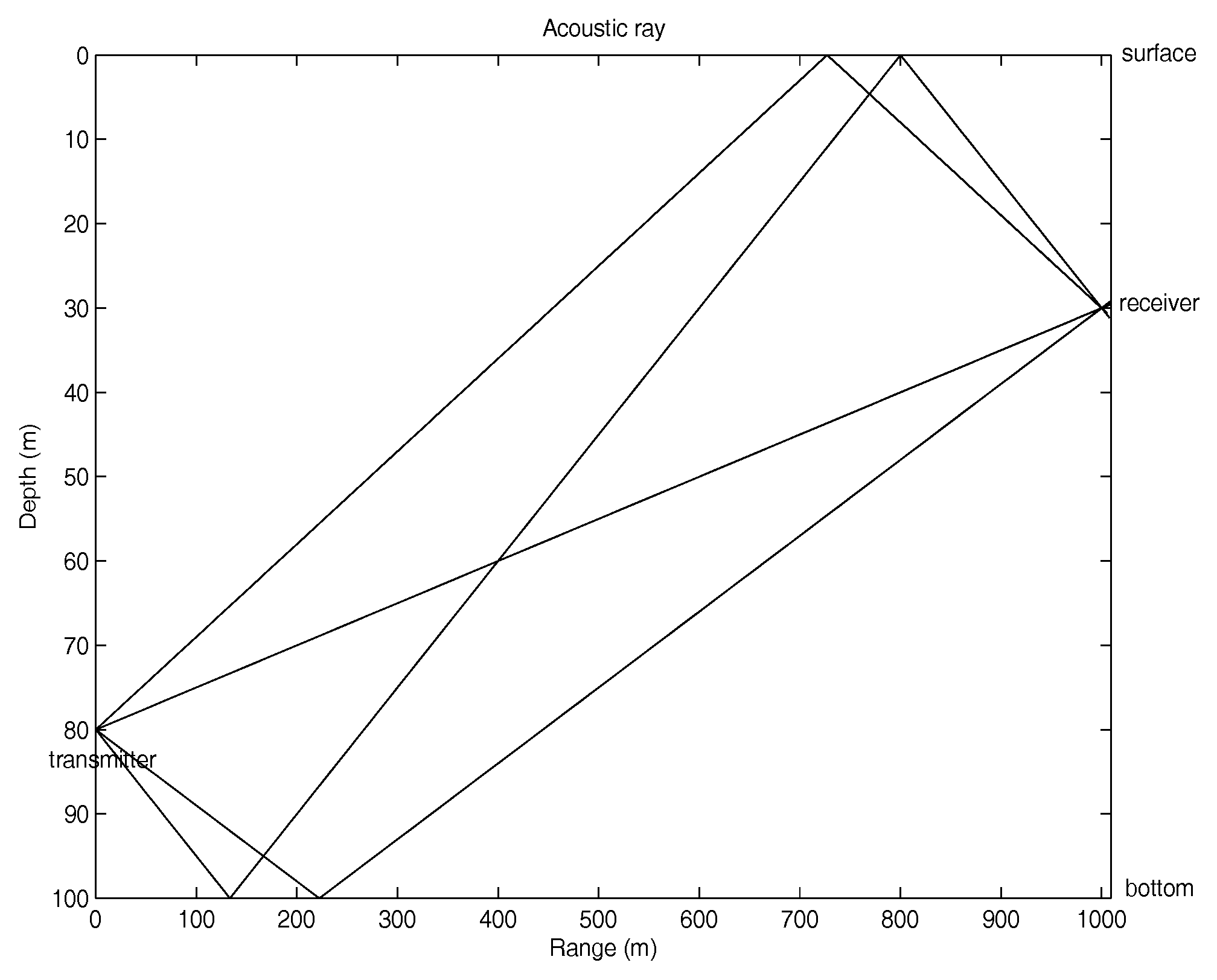
The computer simulation is based on BELLHOP and is implemented in Matlab software. BELLHOP is a beam tracing model for predicting acoustic pressure fields in ocean environments [23]. The underwater environment is set as: the water is 100 m deep, the initial horizontal range between the transmitter and receiver is 1000 m. the transmitter is fixed at the depth of 80 m, and the receiver is at 30 m depth with a horizontal speed of 4.5 m/s toward the transmitter. The speed of the acoustic wave is set to be 1500 m/s. In addition, the reflection coefficients of the bottom and the surface are set to be 0.7 and −0.9, respectively. As shown in Figure 1.
At the receiver, both WT-based algorithm and OMP algorithm will be applied to channel estimation. For WT-based algorithm, WT will be applied twice to search for and at each iteration, while for OMP algorithm, we build a dictionary with a resolution of in the Doppler scale factor and in the tap delay.
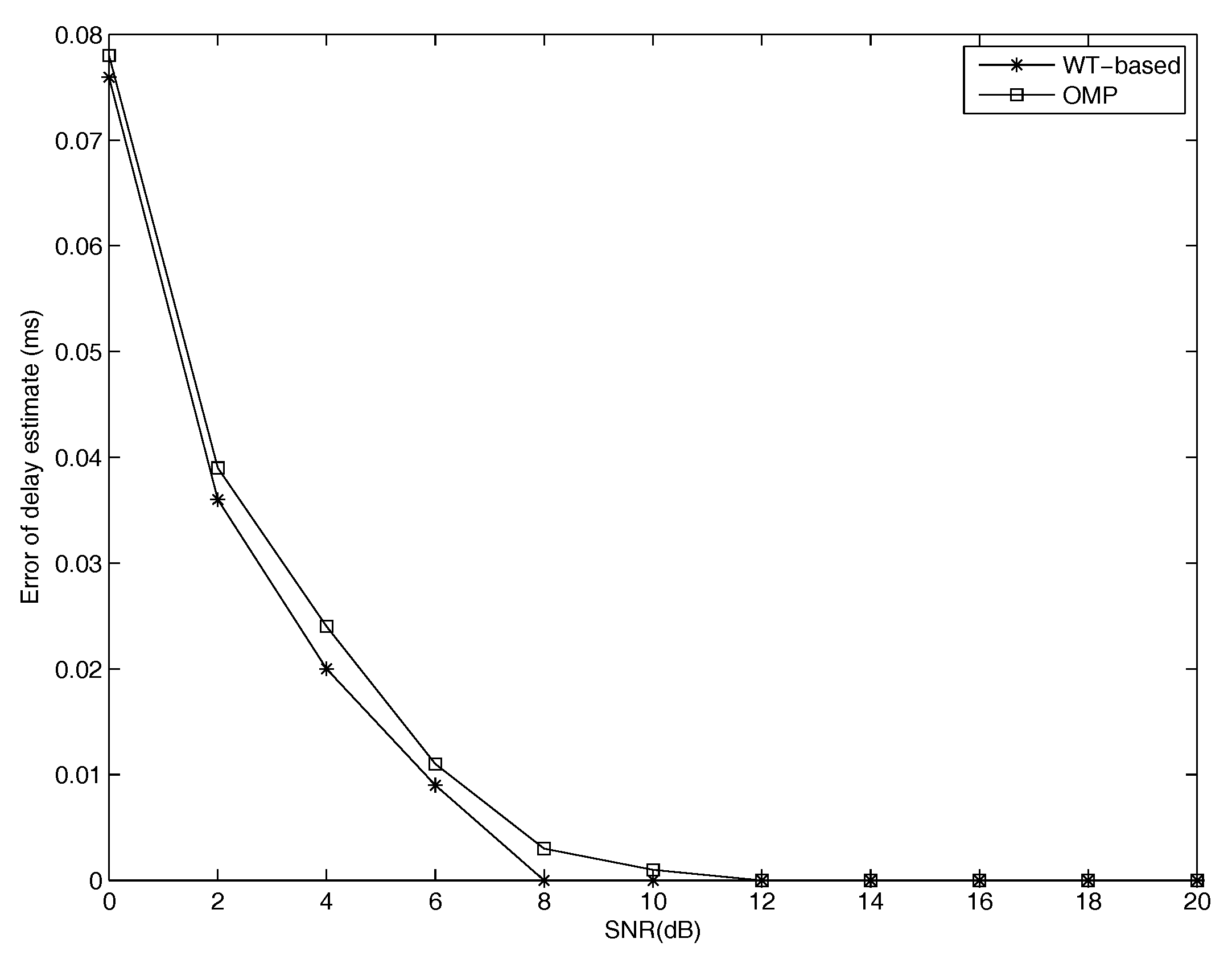
Figure 2 and Figure 3 display the estimating errors of the Doppler scale factor and time delay versus signal to noise ratio (SNR), as defined in the following:
From Figure 2 and Figure 3, we can see that WT-based algorithm is slightly better than OMP algorithm when SNR is lower than 12 dB. In addition, at high SNR, both algorithm can achieve low Doppler scale estimation errors, and the delay estimation errors are nearly 0, which implies that WT-based algorithm is an effective algorithm for channel estimation as the classical OMP algorithm while only needs one-dimension searching.
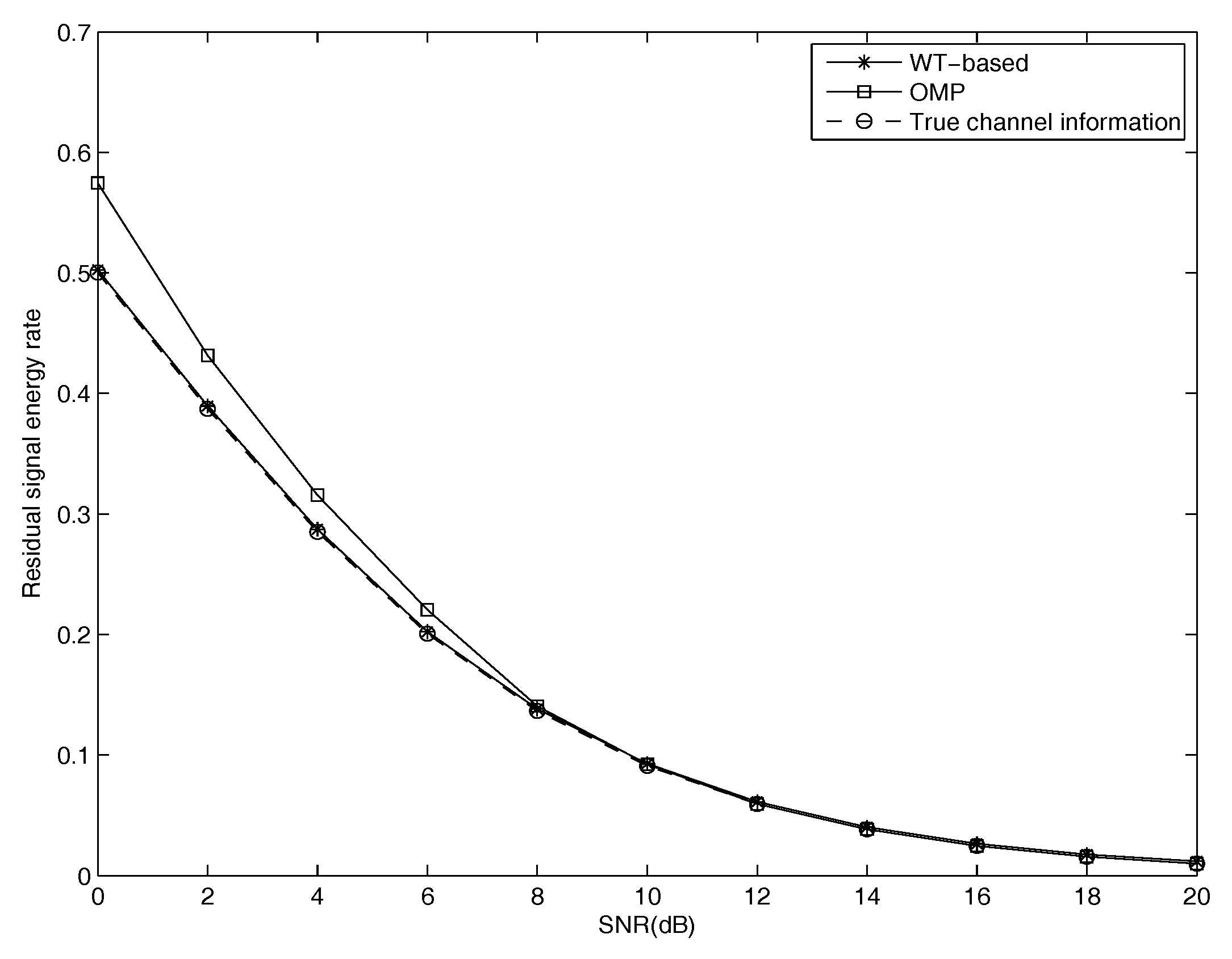
Figure 4 illustrates the residual signal energy rate, , versus SNR of both estimation algorithms. In addition, a reference which uses the true channel information is also included. It shows that the performance of WT-based algorithm approaches to the lower bound while OMP algorithm has some performance losses at low SNR. Residual signal energy rate is a comprehensive evaluation of the channel estimation, that is, the estimation accuracies of Doppler scale, delay and amplitude all contribute to it. Thus the performance in Figure 4 is also coincident with which we analyzed in Figure 2 and Figure 3.
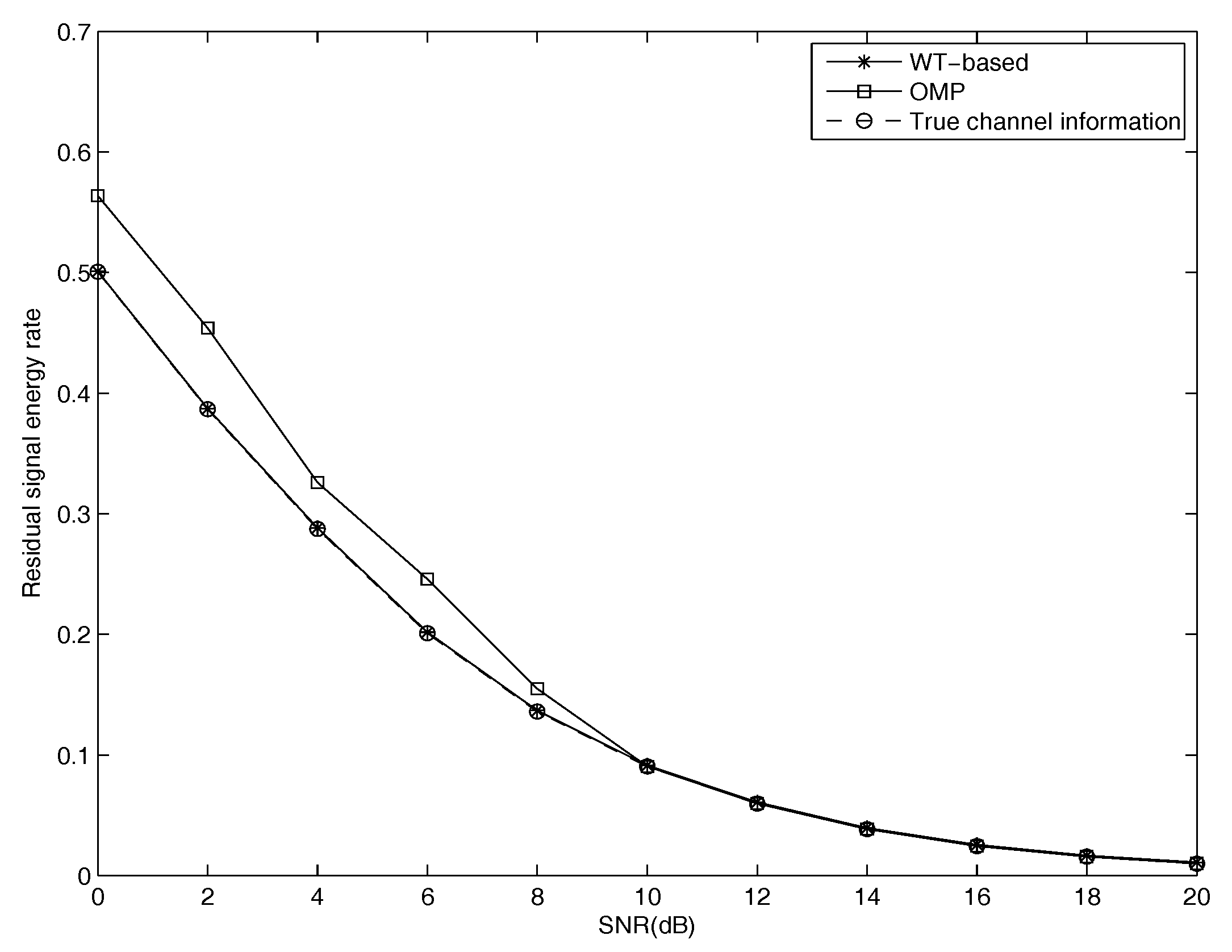
In addition, according to the reviewer’s suggestions, we also include residual signal energy rate versus SNR at different sampling rates: in Figure 5 and in Figure 6. It shows that WT-based algorithm can maintain good performances at different sampling rates, while OMP algorithm shows performance degradation at low sampling rate.
4.2. Complexity Analysis
Both WT-based and OMP algorithms estimate path parameters iteratively, and for proper selection of , the iteration number is nearly the true channel path number for both of them. Therefore, the mainly differences of computation lie in the process of one iteration. Hence we will focus on the computation of one iteration.
For OMP algorithm, parameters in both time domain and Doppler domain need to be searched. Let be the length of the training sequence, be the grid points on the time dimension, be the grid points on the Doppler scale dimension, thus the column numbers of the dictionary is . Thus, the inner products of the received signal and columns in the dictionary require complex multiplications.
For WT-based algorithm, WT will be performed twice at each iteration. As mentioned before, HFM signal is Doppler invariant, thus it only needs to search in the time domain. let be the length of the training sequence, and be the grid points on the time dimension, and then the computation is .
Therefore, WT-based algorithm only needs one-dimension searching and the computational complexity is much lower than OMP algorithm, especially when the grid points on the Doppler scale dimension is large.
5. Conclusions
We have investigated the problem of doubly spread UWA channels estimation in this paper and proposed the WT-based algorithm. By using the superimposed HFM signal as training signal, the proposed algorithm only needs to search in time domain, and the Doppler scale factor and time delay can be simultaneously estimated. Therefore, it greatly reduce the computational complexity than OMP algorithm, while has slightly better performance.
Acknowledgments
This work was supported by National Basic Research Program of China (973) (Grant No. 2013CB336600), National Natural Science Foundation of China (Grant Nos. 61671144, 61372101, 61521061), National High Technology Research and Development Program of China (863) (Grant No. 2014AA01A704), Fundamental Research Funds for the Central Universities and the Open Research Fund of Key Lab of Broadband Wireless Communications and Sensor Network Technologies (NJUPT), Ministry of Education (Grant No. NYKL201502), Funding of Supporting Excellent Young Professors for Teaching and Research in Southeast University, and Shandong Provincial Natural Science Foundation, China (Grant No. ZR2017BF028).
Author Contributions
The idea of this work was proposed by Xing Zhang; Xing Zhang, Chunguo Li and Luxi Yang designed the framework and the experiments; Xing Zhang and Kang Song analyzed the data and wrote the paper; Chunguo Li and Luxi Yang helped revise the paper.
Conflicts of Interest
The authors declare no conflict of interest.
Abbreviations
The following abbreviations are used in this manuscript:
| UWA | Underwater Acoustic |
| MSML | Multi-scale Multi-lag |
| OMP | Orthogonal Matching Pursuit |
| WT | Wavelet Transform |
| HFM | Hyperbolic Frequency Modulation |
| SNR | Signal to Noise Ratio |
| ISI | Inter-symbol Interference |
| CS | Compressed-sensing |
| BP | Basis Pursuit |
| MP | Matching Pursuit |
| SaMP | Sparsity adaptive Matching Pursuit |
| AS-SaMP | Adaptive Step size Sparsity adaptive Matching Pursuit |
| FFT | Fast Fourier Transform |
| CWT | Continuous Wavelet Transform |
| DWT | Discrete Wavelet Transform |
Appendix A
Let be the transmitted HFM signal and expressed as
The definitions of variables in (A1) are the same as in (4). In addition, we assume that the channel has L paths, with as the path amplitude, Doppler scale factor and time delay of the path. Then the received signal without considering noise is as follows:
The instantaneous frequency of the received signal from path is
According to (8), there is a constant time shift which makes the establishment of the following formula:
where
At the receiver, we use the transmitted HFM signal as the mother wave. With the scale and time shift b, it can be written as
In addition, the instantaneous frequency of is
Comparing with (A3), we can find that, by setting , WT coefficients will meet a peak at .
Appendix B
Let be a HFM down sweep signal and the received signal from one path without considering noise is:
In addition, the instantaneous frequency of is
When use the HFM up sweep signal as the mother wave and set , the instantaneous frequency is:
Suppose there is a constant time shift b which can make the establishment of the following formula:
By solving (A10), we can obtain that
where is the Doppler scale factor, when the transmitter and the receiver are approaching each other; when they are away from each other; and when they are static. Therefore and b varies with t. The assumption that b is constant is incorrect. In addition, it is the same for .
References
- Akyildiz, I.F.; Pompili, D.; Melodia, T. Challenges for efficient communication in underwater acoustic sensor networks. ACM Sigbed Rev. 2004, 1, 3–8. [Google Scholar] [CrossRef]
- Mason, S.; Berger, C.; Zhou, S.; Willett, P. Detection, Synchronization, and Doppler Scale Estimation with Multicarrier Waveforms in Underwater Acoustic Communication. IEEE J. Sel. Areas Commun. 2008, 26, 1638–1649. [Google Scholar] [CrossRef]
- Singer, A.C.; Nelson, J.K.; Kozat, S.S. Signal processing for underwater acoustic communications. Commun. Mag. IEEE 2009, 47, 90–96. [Google Scholar] [CrossRef]
- Qu, F.; Wang, Z.; Yang, L.; Wu, Z. A journey toward modeling and resolving doppler in underwater acoustic communications. IEEE Commun. Mag. 2016, 54, 49–55. [Google Scholar] [CrossRef]
- Tao, J. Single-Carrier Frequency-Domain Turbo Equalization With Various Soft Interference Cancellation Schemes for MIMO Systems. IEEE Trans. Commun. 2015, 63, 3206–3217. [Google Scholar] [CrossRef]
- Mason, S.F.; Berger, C.R.; Zhou, S.; Ball, K.R. Receiver comparisons on an OFDM design for Doppler spread channels. In Proceedings of the 2009 OCEANS Europe Conference, Bremen, Germany, 11–14 May 2009; pp. 1–7. [Google Scholar] [CrossRef]
- Berger, C.R.; Zhou, S.; Preisig, J.C.; Willett, P. Sparse channel estimation for multicarrier underwater acoustic communication: From subspace methods to compressed sensing. IEEE Trans. Signal Process. 2010, 58, 1708–1721. [Google Scholar] [CrossRef]
- Xu, T.; Tang, Z.; Leus, G.; Mitra, U. Multi-Rate Block Transmission Over Wideband Multi-Scale Multi-Lag Channels. IEEE Trans. Signal Process. 2013, 61, 964–979. [Google Scholar] [CrossRef]
- Daoud, S.; Ghrayeb, A. Using Resampling to Combat Doppler Scaling in UWA Channels with Single-Carrier Modulation and Frequency-Domain Equalization. IEEE Trans. Veh. Technol. 2016, 65, 1261–1270. [Google Scholar] [CrossRef]
- Cotter, S.F.; Rao, B.D. Sparse channel estimation via matching pursuit with application to equalization. IEEE Trans. Commun. 2002, 50, 374–377. [Google Scholar] [CrossRef]
- Tropp, J.A.; Gilbert, A.C. Signal Recovery From Random Measurements Via Orthogonal Matching Pursuit. IEEE Trans. Inf. Theory 2007, 53, 4655–4666. [Google Scholar] [CrossRef]
- Do, T.T.; Lu, G.; Nguyen, N.; Tran, T.D. Sparsity adaptive matching pursuit algorithm for practical compressed sensing. In Proceedings of the 2008 Asilomar Conference on Signals, Systems and Computers, Pacific Grove, CA, USA, 26–29 October 2009; pp. 581–587. [Google Scholar] [CrossRef]
- Zhang, Y.; Venkatesan, R.; Dobre, O.A.; Li, C. An adaptive matching pursuit algorithm for sparse channel estimation. In Proceedings of the 2015 IEEE Wireless Communications and Networking Conference (WCNC), New Orleans, LA, USA, 9–12 March 2015; pp. 626–630. [Google Scholar] [CrossRef]
- Qu, F.; Nie, X.; Xu, W. A Two-Stage Approach for the Estimation of Doubly Spread Acoustic Channels. IEEE J. Ocean. Eng. 2015, 40, 131–143. [Google Scholar] [CrossRef]
- Yu, F.; Li, D.; Guo, Q.; Wang, Z.; Xiang, W. Block-FFT Based OMP for Compressed Channel Estimation in Underwater Acoustic Communications. IEEE Commun. Lett. 2015, 19, 1937–1940. [Google Scholar] [CrossRef]
- Zhang, L.; Xu, X.; Feng, W.; Chen, Y. HFM spread spectrum modulation scheme in shallow water acoustic channels. In Proceedings of the 2013 MTS/IEEE OCEANS Conference, Hampton Roads, VA, USA, 14–19 October 2013; pp. 1–6. [Google Scholar] [CrossRef]
- Yang, J.; Sarkar, T.K. A New Doppler-Tolerant Polyphase Pulse Compression Codes Based on Hyperbolic Frequency Modulation. In Proceedings of the 2007 IEEE Radar Conference, Boston, MA, USA, 17–20 April 2007; pp. 265–270. [Google Scholar] [CrossRef]
- Ai, J.; Wang, Z.; Zhou, X.; Ou, C. Improved wavelet transform for noise reduction in power analysis attacks. In Proceedings of the 2017 IEEE International Conference on Signal and Image Processing, Beijing, China, 13–15 August 2017; pp. 602–606. [Google Scholar] [CrossRef]
- Yang, C.; Liang, H. Time-scale analysis of wideband HFM signal and application on moving target detection. In Proceedings of the ICIEA 2009 IEEE Conference on Industrial Electronics and Applications, Xi’an, China, 25–27 May 2009; pp. 3887–3890. [Google Scholar] [CrossRef]
- Burhan, N.; Kasno, M.; Ghazali, R. Feature extraction of surface electromyography (sEMG) and signal processing technique in wavelet transform: A review. In Proceedings of the IEEE International Conference on Automatic Control and Intelligent Systems, Selangor, Malaysia, 22–22 October 2017; pp. 141–146. [Google Scholar] [CrossRef]
- Young, R.K. Wavelet Theory and Its Applications; Springer: Berlin, Germany, 1996; Volume 189, pp. 19–22. [Google Scholar] [CrossRef]
- Agrawal, S.; Dhend, M.H. Wavelet transform based voltage quality improvement in smart grid. In Proceedings of the International Conference on Automatic Control and Dynamic Optimization Techniques, Pune, India, 9–10 September 2017; pp. 289–294. [Google Scholar] [CrossRef]
- Gul, S.; Zaidi, S.S.H.; Khan, R.; Wala, A.B. Underwater acoustic channel modeling using BELLHOP ray tracing method. In Proceedings of the International Bhurban Conference on Applied Sciences and Technology, Islamabad, Pakistan, 10–14 January 2017; pp. 665–670. [Google Scholar] [CrossRef]
Figure 1.
Acoustic ray paths of UWA channel.

Figure 2.
Errors of the estimating Doppler scale factor versus SNR.

Figure 3.
Errors of the estimating delay versus SNR.

Figure 4.
Residual signal energy rate versus SNR.

Figure 5.
Residual signal energy rate versus SNR with sampling rate at 20 kHz.
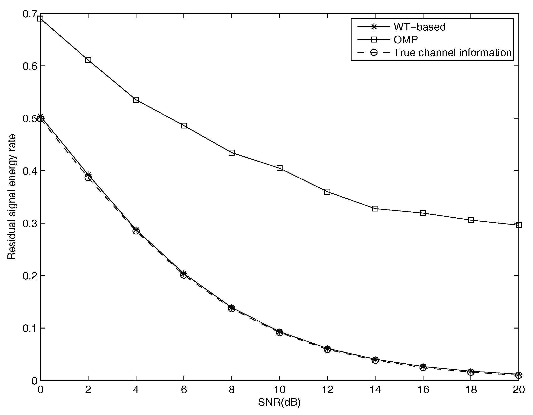
Figure 6.
Residual signal energy rate versus SNR with sampling rate at 60 kHz.

© 2018 by the authors. Licensee MDPI, Basel, Switzerland. This article is an open access article distributed under the terms and conditions of the Creative Commons Attribution (CC BY) license (http://creativecommons.org/licenses/by/4.0/).
Share and Cite
MDPI and ACS Style
Zhang, X.; Song, K.; Li, C.; Yang, L. A Novel Approach for the Estimation of Doubly Spread Acoustic Channels Based on Wavelet Transform. Appl. Sci. 2018, 8, 38. https://doi.org/10.3390/app8010038
AMA Style
Zhang X, Song K, Li C, Yang L. A Novel Approach for the Estimation of Doubly Spread Acoustic Channels Based on Wavelet Transform. Applied Sciences. 2018; 8(1):38. https://doi.org/10.3390/app8010038
Chicago/Turabian StyleZhang, Xing, Kang Song, Chunguo Li, and Luxi Yang. 2018. "A Novel Approach for the Estimation of Doubly Spread Acoustic Channels Based on Wavelet Transform" Applied Sciences 8, no. 1: 38. https://doi.org/10.3390/app8010038
Note that from the first issue of 2016, this journal uses article numbers instead of page numbers. See further details here.