Application of the Wave Propagation Approach to Sandwich Structures: Vibro-Acoustic Properties of Aluminum Honeycomb Materials

Featured Application

Acoustic design and characterization of sandwich panels.

Abstract

Sandwich structures are manufactured using multiple combinations of materials for core and laminates. The real performances are influenced by variability in the composing layers and even by the uncertainties introduced while bonding them together. Therefore, experimental tests are usually the preferred way to assess the most important parameters required to develop and to characterize the product, the main downsides lying in their cost and time consumption. This work explores a practical application of the wave propagation approach by means of a case study, in which some significant properties of an aluminum honeycomb panel are obtained starting from simple vibro-acoustic tests carried out on beam specimens. After determining the frequency-dependent bending stiffness function, the sound transmission loss is predicted and compared with the experimental results obtained in sound transmission suites. The same vibro-acoustic tests are used to estimate the core shear modulus. Finally, a parametric study is proposed to show how this technique can be effectively used in the early design stage, when producing physical samples is often impossible due to time and money constraints. The method proved to be a reliable and powerful tool in all the tested applications, providing good results with limited computational effort.

1. Introduction

The study of materials is in many fields a key to improve performances. In this respect, composite structures are a class of interesting products allowing one to combine the properties of various individual materials to obtain a new material with enhanced characteristics. The construction of aerospace structures has historically been one of the driving forces behind the development of advanced composite materials, making large use of foam and honeycomb aluminum panels because of aluminum’s high strength-to-weight ratio, energy absorption, heat transfer and electromagnetic shielding properties, combined with good machinability at a relatively low cost [1]; all qualities that spread the diffusion of such structures to the transportation sector, including rail [2] and shipbuilding [3] industries where the characteristics have to satisfy lightweight and structural demands. The characterization of aluminum honeycomb structures has been the subject of many scientific works, especially from the mechanical viewpoint [4,5] and, in recent years, for innovative types of core [6,7] for which experimental results must validate virtual models. Frequency-dependent dynamic and acoustic performances are other important aspects to consider when choosing or designing the materials to be used, as shown in [8,9,10].

Although the ability of building new products from the combination of different layers seems to be unlimited, sandwich structures have always been considered as challenging materials, and the challenge is two-fold: on the one hand, to make such materials easy to produce at the industrial scale without sacrificing performances and taking into account possible problems due to the manufacturing technology [11,12] and, on the other hand, to be able to design, characterize and quality-check them by using new approaches [13] able to give a good description of the behavior also under non-standard conditions (see for instance [14]). For this reason, this enormous potential is rarely fully exploited in civilian sectors mainly due to the cost of design, prototype-making and testing activities, thus sticking to off-the-shelf options that do not completely fulfil the application requirements. In this respect, creating instruments allowing one to reduce the time and costs of early engineering steps becomes of great importance.

The wave propagation approach is a powerful tool to predict the flexural behavior and vibrational response of complex structures, which can be used as a starting point to estimate their sound insulation properties with relatively simple experimental data required and low computational efforts [15,16,17] if compared with FEM simulations. The model is based on the concept of the frequency-dependent bending stiffness function, derived from the bending wave propagation inside thin beams or plates. Some application examples of the wave propagation approach using also a frequency-dependent Young’s modulus for describing the laminate properties can be found in [18].

The aim of the present paper is to show the potentiality of this approach to find some dynamic, sound insulation and mechanical properties of complex materials, by means of a case study. Starting from the model equations and simple modal measurements, the bending stiffness, the sound transmission loss and the shear modulus of an aluminum honeycomb sandwich panel are determined. Simulation results are validated by means of sound transmission suites and mechanical tests. Finally, a parametric study is carried out to show how this method can be used to design sandwich materials based on plain ‘datasheet’ properties.

2. Theory

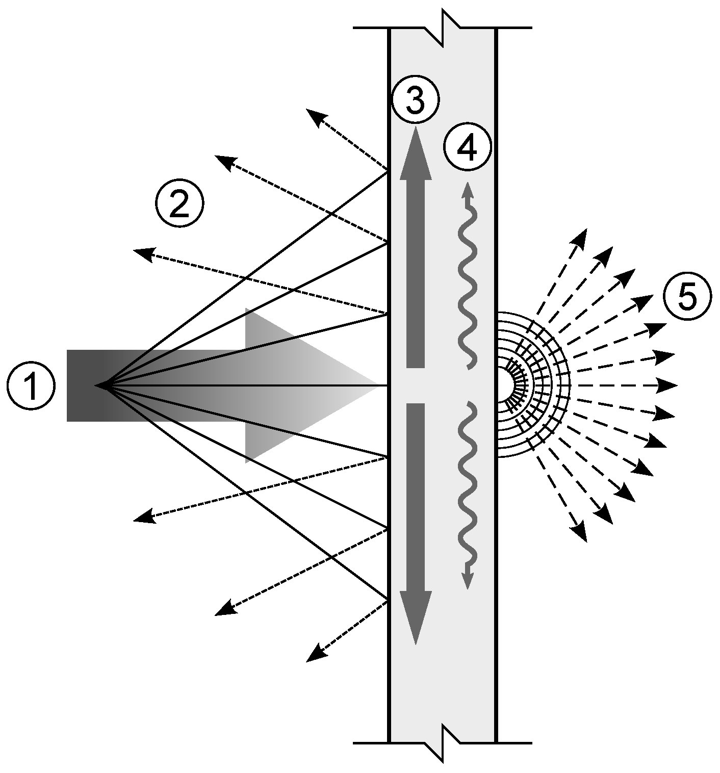
2.1. Sound Propagation through a Partition

When a sound wave having a certain power $W_0$ impinges a wall (Figure 1), some of the power is reflected back ($W_r$), and some of it propagates beyond the surface and is partially dissipated into heat (internal losses $W_d$) and partially distributed across the junctions to the adjacent structures (losses due to transmission to the adjacent structures $W_{t^{\prime }}$). This part is related to flanking transmissions. Finally, a portion of the power crosses the partition and is transmitted along a direct path across the wall ($W_t$).

The two terms $W_t$ and $W_{t^{\prime }}$ represent the portion of the acoustic power transmitted to the adjacent structures and can be put together into a single term $W_{t,tot}$. Considering a small element of the wall, it is possible to write an equation representing the power balance over the element:

$$W_0=W_r+W_d+W_{t,tot}.$$

(1)

Dividing both terms by $W_0$, Equation (1) can be rewritten as:

$$1=r+\delta +\tau ,$$

(2)

where r is the reflection coefficient, $\delta$ is the dissipation coefficient and $\tau$ is the transmission coefficient. The ‘apparent’ sound absorption coefficient, $\alpha$, is defined as the sum of the dissipated and transmitted power fractions. Since both of them depend on the angle of incidence of the sound on the surface, different $\alpha$-values can be obtained for the same type of material according to the adopted measurement technique [19]. The transmission coefficient $\tau$ is also related to the sound transmission loss R:

$$R=10{log}_{10}\left(\frac{1}{\tau }\right),$$

(3)

and its determination is therefore the key to describe the sound insulation properties of a partition. Coefficient $\tau$ is a function of the angle of incidence, the mass per unit area, the bending stiffness and the total losses. The next sections will provide a background theory for the propagation of bending waves through partitions, which forms the basis for the calculation method of the transmission coefficient in composite structures.

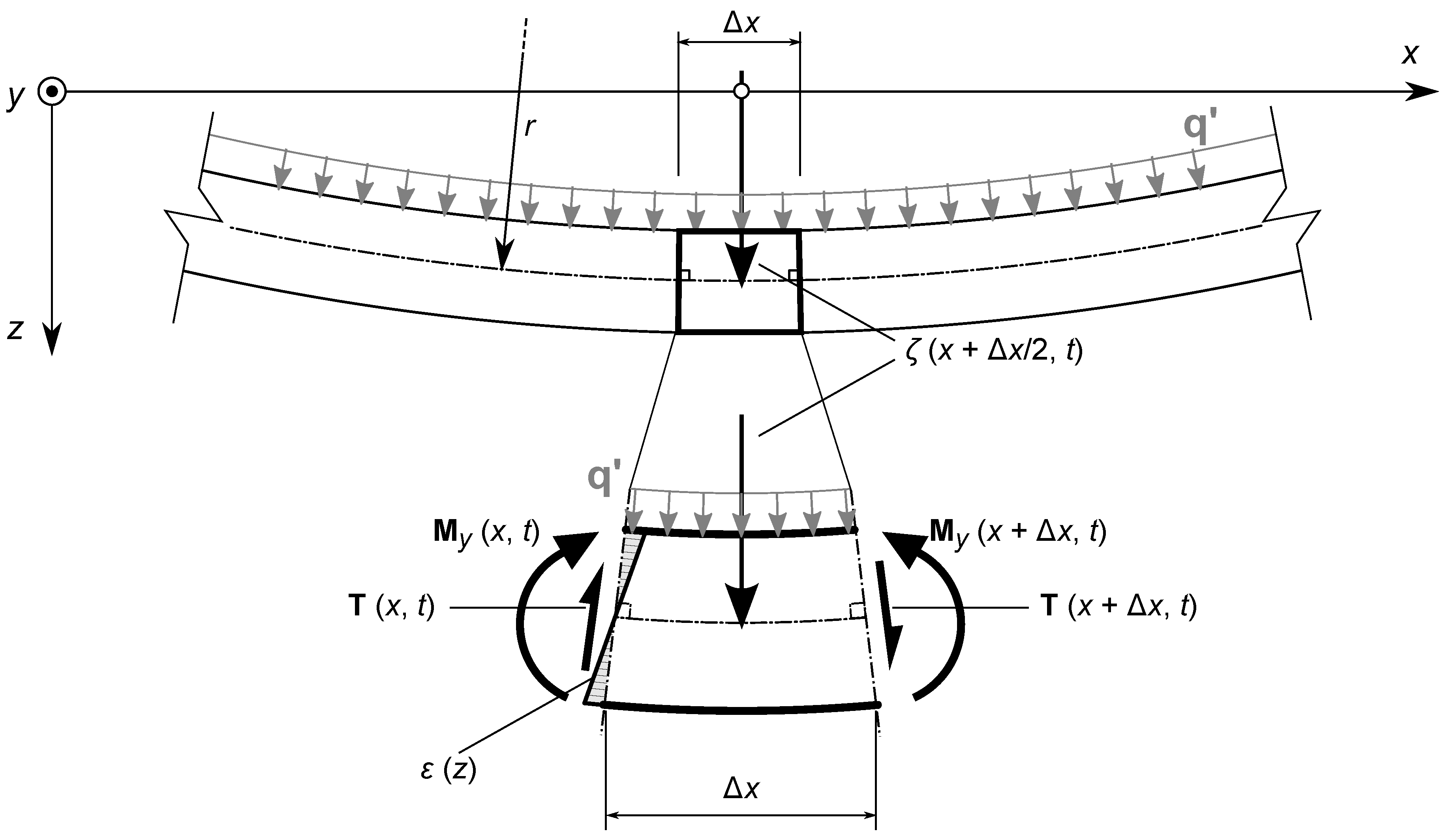
2.2. Propagation of Bending Waves

The simplest type of partition for which it is possible to determine the sound transmission loss is a homogeneous wall. In this case, a simplified theory can be applied, once the bending stiffness of the structure is obtained either theoretically or experimentally. Before discussing the model related to the estimation of the sound transmission loss, the background on the propagation of the bending waves in thin plates must be established. The complete presentation can be found in [20] and will be summarized here.

When the sound impinges one side of a plate, vibrations are induced in the partition, and the partition develops bending waves. Let us consider a straight and thin beam bending in the $\left(x,z\right)$ plane as shown in Figure 2, where $\zeta$ is the lateral displacement due to bending. It is possible to derive a differential equation to describe the propagation of the bending waves starting from the equation of motion applied to a small portion of beam having a length $\Delta x$. When the beam bends, the different fiber layers and the axis undergo a bending motion, as well. Consequently, some shear and traction/compression forces are induced in the beam.

Assuming that plane sections remain plain and perpendicular to the axis, thus neglecting the deformations produced by the shearing forces, the normal stress over the cross-section can be written as $\sigma =E\times \epsilon \left(z\right)$, where E is the Young’s modulus of the material, and the classic Euler–Bernoulli theory of ‘pure bending waves’ is derived. This assumption can generally be accepted when the bending wavelength is large if compared with the cross-sectional dimensions. In this condition, the bending moment ${\mathbf{M}}_y$ can be obtained as:

$${\mathbf{M}}_y={\int }_S\sigma z\mathrm{d}S={\int }_{S}E\times \epsilon \left(z\right)z\mathrm{d}S\approx -E\frac{{\partial }^2\zeta }{\partial x^2}{\int }_S{z}^2\mathrm{d}S=-E{I}_b\frac{{\partial }^2\zeta }{\partial x^2}$$

(4)

where $I_b$ is the moment of inertia relative to the beam cross-section S. Since the bending stiffness D is the proportionality constant in the relation between the bending moment ${\mathbf{M}}_y$ and the curvature, ${\partial }^2\zeta /\partial x^2$, it can be defined as:

$$D=E{I}_b.$$

(5)

The sound insulation characteristics of the material are strongly related to its flexural behavior. The bending wave phase velocity in an isotropic panel, $c_B$, is frequency-dependent and can be expressed as:

$$c_B=\sqrt[4]{\frac{{\left(2\pi f\right)}^{2}D}{\mu }}$$

(6)

where $\mu$ is the mass per unit area of the wall. When the incident sound waves have the same trace wavelength as free bending waves, the so-called ‘coincidence effect’ occurs. In this region, the bending wave speed is equal to the speed of sound in air, $c_{air}$, the wall oscillations are amplified and the acoustic waves are directly transmitted almost without attenuation. The critical frequency, $f_c$, is related to D and is defined as the lowest frequency for which the coincidence effect occurs, that is the frequency at which the bending wave becomes supersonic:

$$f_c=\left(\frac{c_{air}^2}{2\pi }\right)\sqrt{\frac{\mu }{D}}.$$

(7)

Cremer [21] derived the sound transmission coefficient $\tau \left(\phi ,\omega \right)$ for a infinite thin homogeneous plate as a function of the angle of incidence $\phi$ of the acoustic wave and of the angular frequency, $\omega =2\pi f$:

$$\begin{array}{ccc}\hfill \tau \left(\phi \right)& =& \left\{{\left[1+\frac{\mu \omega }{2\rho c}cos\phi \times {\left(\frac{f}{f_c}\right)}^2{\left(sin\phi \right)}^4\eta \right]}^2+\right.\hfill \\ & & {\left.+{\left[\frac{\mu \omega }{2\rho c}cos\phi \times \left\{{\left(\frac{f}{f_c}\right)}^2{\left(sin\phi \right)}^4-1\right\}\right]}^2\right\}}^{-1}.\hfill \end{array}$$

(8)

Here, $\rho c$ is the wave impedance of the surrounding medium at room temperature (415 kg m${}^{-2}$ s${}^{-1}$ for air), while ${\eta }_{tot}$ represents the total loss factor of the structure (see Section 2.5). The sound transmission coefficient must therefore be integrated over the incidence angle range to obtain the sound transmission coefficient for diffuse incidence:

$${\tau }_d=2{\int }_0^{{\phi }_{lim}}\tau \left(\phi \right)\times cos\phi sin\phi \mathrm{d}\phi$$

(9)

Assuming that, for a perfectly diffuse field, the angles of incidence are equally probable, the integration should be performed between 0${}^{\circ }$ and 90${}^{\circ }$. However, comparisons between predicted and measured sound transmission loss values showed that the limitation of the integration range to a ${\phi }_{lim}$ = 78${}^{\circ }$–85${}^{\circ }$ generally provides better agreement, the common explanation being that the sound field in sound transmission suites is not perfectly diffuse and grazing angles are characterized by less incident energy [22]. The result of the integration can be used to compute the sound transmission loss as a function of frequency, by means of Equation (3). In homogeneous walls, the bending stiffness D is a constant and can be computed with Equation (5).

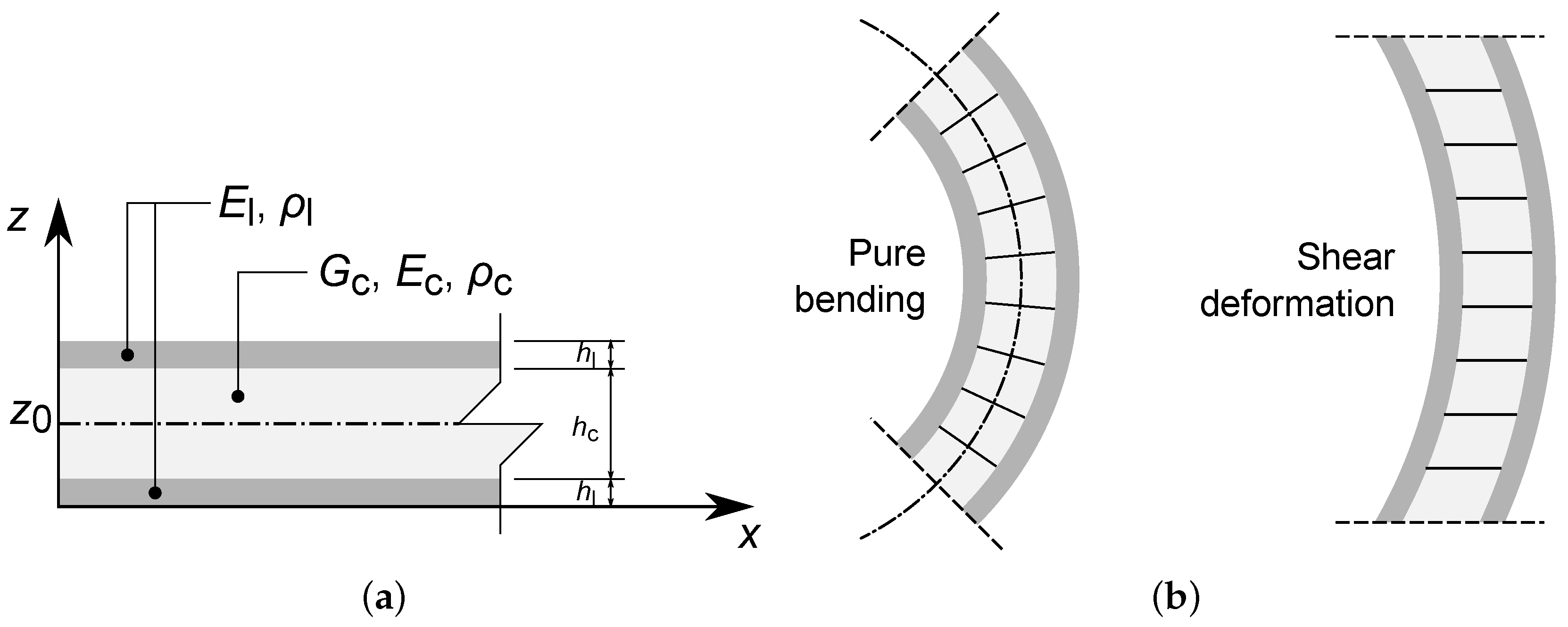
2.3. From Homogeneous to Sandwich Partitions

Switching from a homogeneous to a sandwich partition changes the dynamic behavior of the wall considerably, as demonstrated by several extensions on the original Euler–Bernoulli theory aiming at making it applicable to thick, more complex partitions. Reviews of some of these pioneering studies can be found for instance in [23,24]. In 1990, a sophisticated model describing the lateral displacement of sandwich beams featuring thick core and thin laminates has been proposed by Nilsson [25], featuring a complex set of ill-conditioned equations that could be solved only with considerable numerical effort. When such a fine level of detail is not required, as in most practical applications, the use of simpler methods can be investigated. In particular, the present work uses the model introduced in 2002 by Nilsson and Nilsson [26], who proposed a different approach based on the formulation of the differential equation governing the motion of a sandwich beam according to Hamilton’s principle. The derivation of the model is summarized in the following.

Hamilton’s principle states that the action integral of a mechanical system, expressed as the integral of the difference between kinetic and potential energy, is stationary. In order to write the founding equation of the model, the laminates are assumed to move in phase. Moreover, pure bending of the complete beam and core shear effects are considered (Figure 3b).

The potential energy results as the sum of five contributions: pure bending of the complete beam, shear of the core, bending of the laminates induced by core shear effects and external loads $F^{\prime }$. Kinetic energy is the sum of two contributions, deriving from lateral and rotational motion of the beam. The resulting formulation of the variational problem leads to a set of differential equations that can be rearranged in a single sixth-order equation in the variable $\zeta$ and the relative boundary conditions. For the beam represented in Figure 3a, the governing equation is:

$$\begin{array}{c}\hfill \begin{array}{c}-2D_1^{\prime }{D}_2^{\prime }\frac{{\partial }^6\zeta }{\partial x^6}+2D_2^{\prime }{I}_{\omega }^{\prime }\frac{{\partial }^6\zeta }{\partial x^4\partial t^2}+G_{c}S{D}_1^{\prime }\frac{{\partial }^4\zeta }{\partial x^4}-\left[\left(D_1^{\prime }+2D_2^{\prime }\right)m^{\prime }+G_{c}S{I}_{\omega }^{\prime }\right]\frac{{\partial }^4\zeta }{\partial x^2\partial t^2}+\hfill \\ +G_{c}S{m}^{\prime }\frac{{\partial }^2\zeta }{\partial t^2}+m^{\prime }{I}_{\omega }^{\prime }\frac{{\partial }^4\zeta }{\partial t^4}=G_{c}S{F}^{\prime }-\left(D_1^{\prime }+2D_2^{\prime }\right)\frac{{\partial }^2{F}^{\prime }}{\partial x^2}+I_{\omega }^{\prime }\frac{{\partial }^2{F}^{\prime }}{\partial t^2}.\hfill \end{array}\end{array}$$

(10)

Here, $G_c$ is the effective shear modulus of the core, $I_{\omega }^{\prime }$ is the mass moment of inertia of the beam and $m^{\prime }$ is its mass per unit length, which for a given width b, is calculated as $\mu ·b$. $D_2^{\prime }$ and $D_1^{\prime }$ are the bending stiffnesses of the beam and of one laminate, respectively:

$$D_1^{\prime }=b\left[\frac{E_c{h}_c^3}{12}+E_l\left(\frac{h_c^2{h}_l}{2}+h_c{h}_l^2+2\frac{h_l^3}{3}\right)\right],$$

(11)

$$D_2^{\prime }=b\frac{E_l{h}_l^3}{12}.$$

(12)

Assuming a solution in the form:

$$\zeta =exp\left[\mathrm{i}\left(\omega t-k_{x}x\right)\right]$$

(13)

and setting the external load $F^{\prime }$ to zero, the dispersion equation relating the wavenumber $k_x$ and the angular frequency $\omega$ is obtained:

$$\begin{array}{c}\hfill \begin{array}{c}2D_1^{\prime }{D}_2^{\prime }{k}_x^6-2D_2^{\prime }{I}_{\omega }^{\prime }{k}_x^4{\omega }^2-\left[m^{\prime }\left(D_1^{\prime }+2D_2^{\prime }\right)+I_{\omega }^{\prime }{G}_{c}S\right]k_x^2{\omega }^2+\hfill \\ +G_{c}S\left[D_1^{\prime }{k}_x^4-m^{\prime }{\omega }^2\right]+m^{\prime }{I}_{\omega }^{\prime }{\omega }^4=0.\hfill \end{array}\end{array}$$

(14)

Equation (14) has six solutions: $k_x$ = $\pm {\kappa }_1$, $\pm \mathrm{i}{\kappa }_2$ and $\pm \mathrm{i}{\kappa }_3$. Figure 4 shows an example of wavenumbers (absolute values) obtained from Equation (14).

${\kappa }_1$ is the wavenumber associated with the first propagating wave. This number is bounded by two limits: a lower asymptote describing the flexural wave in a slender Euler beam and an upper asymptote describing the flexural wave in a laminate:

$$\begin{array}{cc}\hfill \underset{f\to 0}{lim}\left|{\kappa }_1\right|={\left(\frac{m^{\prime }{\omega }^2}{D_1^{\prime }}\right)}^{1/4};& \hfill \underset{f\to \infty }{lim}\left|{\kappa }_1\right|={\left(\frac{m^{\prime }{\omega }^2}{2D_2^{\prime }}\right)}^{1/4}.\end{array}$$

(15)

Therefore, the model proposes to consider the structure as an ‘equivalent’ homogeneous beam having the same dynamic properties as the sandwich beam at hand. If a frequency-dependent ‘apparent’ bending stiffness, $D_a^{\prime }$, is defined, one can write:

$${\kappa }_1^4=\frac{m^{\prime }{\omega }^2}{D_a^{\prime }}.$$

(16)

A discussion of the possible ways to model the apparent bending stiffness and their implications can be found in [27].

Inserting Equation (16) into Equation (14), an equation in $D_a^{\prime }$ is obtained. In the case of honeycomb beams, laminates are generally less stiff than the entire beam, and $D_1^{\prime }\gg D_2^{\prime }$ simplification can be done. If ${\omega }^2{I}_{\omega }^{\prime }\ll G_{c}S$, the motion equation can be further simplified as:

$$\left(\frac{G_{c}S}{\sqrt{m^{\prime }}\omega }\right)\left[\frac{{D_a^{\prime }}^{3/2}}{D_1^{\prime }}-{D_a^{\prime }}^{1/2}\right]+D_a^{\prime }-2D_2^{\prime }=0,$$

(17)

which can be written in the general form:

$$\frac{A}{f}{D_a^{\prime }}^{3/2}-\frac{B}{f}{D_a^{\prime }}^{1/2}+D_a^{\prime }-C=0$$

(18)

once coefficients A, B and C are defined:

$$\begin{array}{ccc}\hfill A=\frac{G_{c}S}{\sqrt{m^{\prime }}2\pi D_1^{\prime }};& \hfill B=\frac{G_{c}S}{\sqrt{m^{\prime }}2\pi };& \hfill C=2D_2^{\prime }.\end{array}$$

(19)

It has been shown that solutions based on this formulation are accurate enough to describe the behavior of a sandwich structure in several practical applications [15,26].

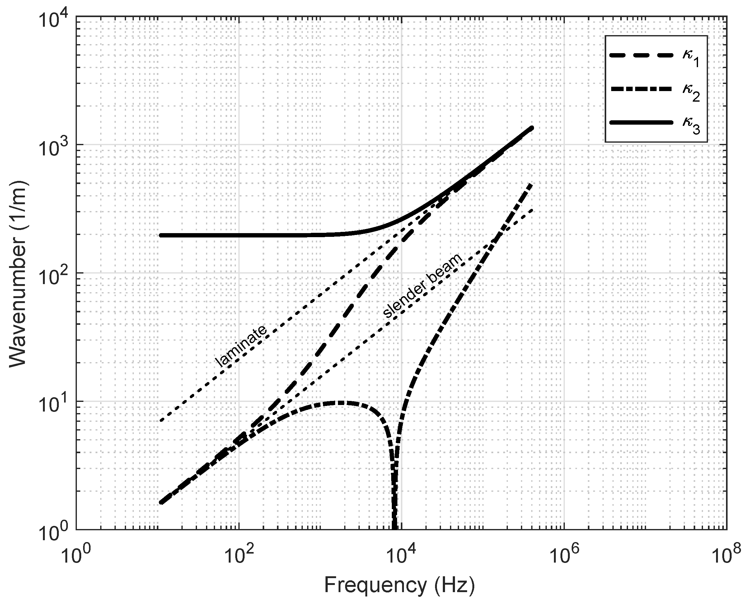
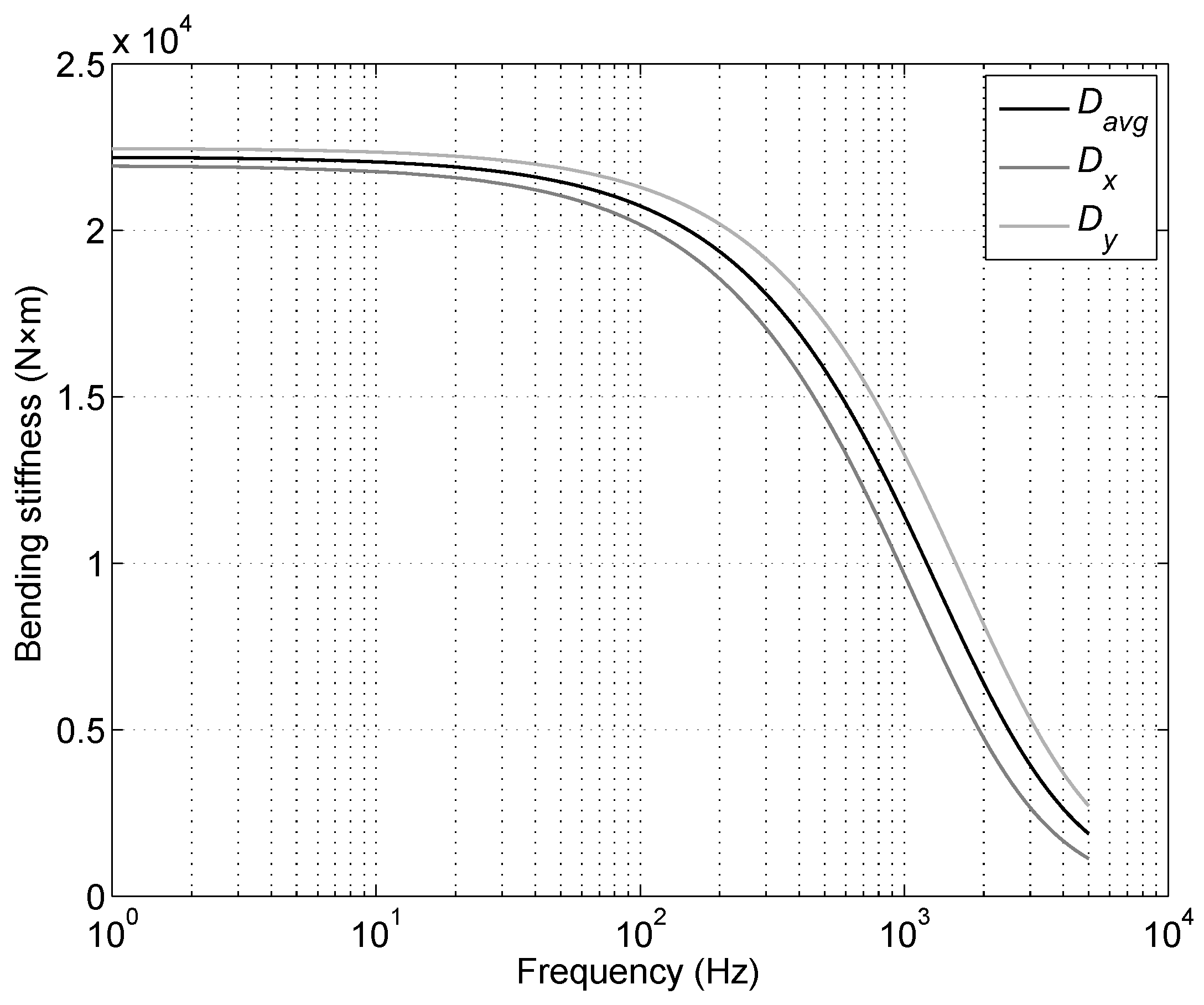
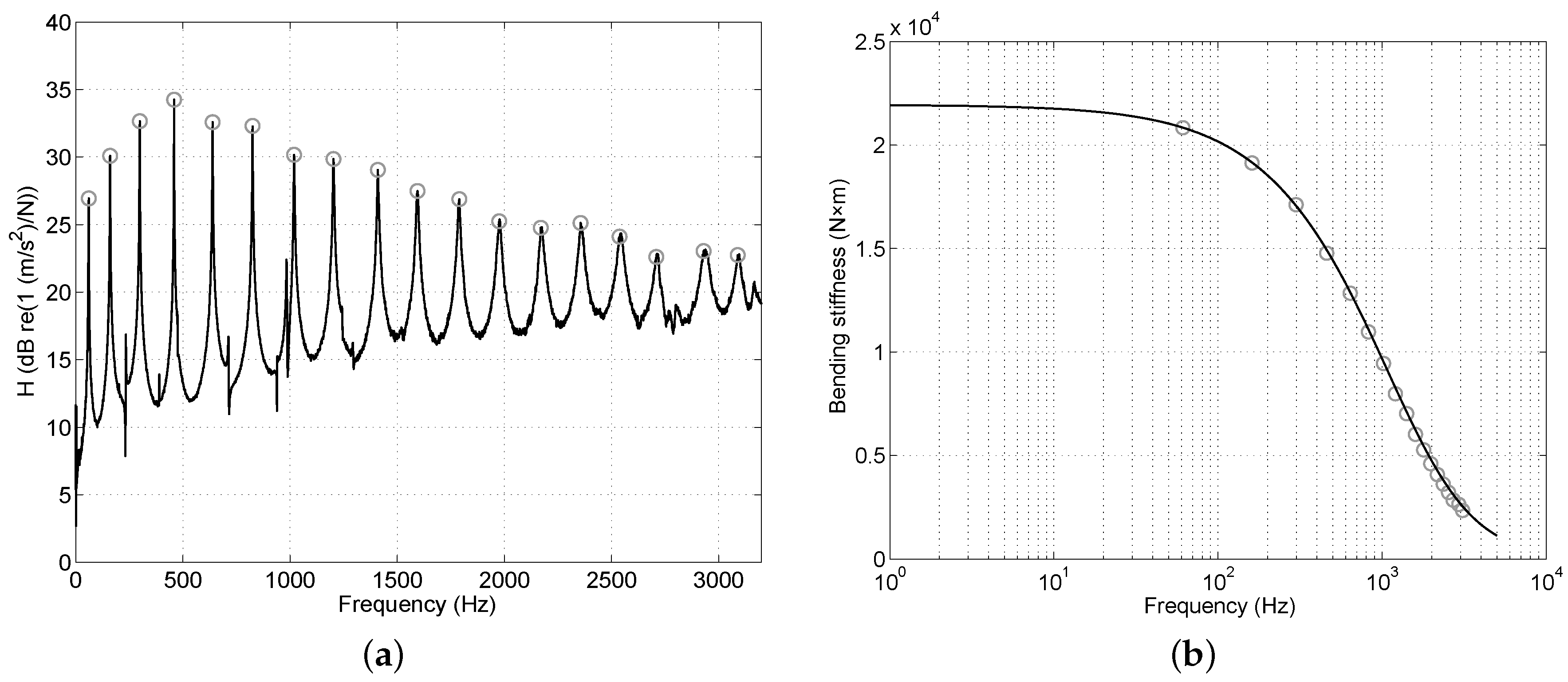
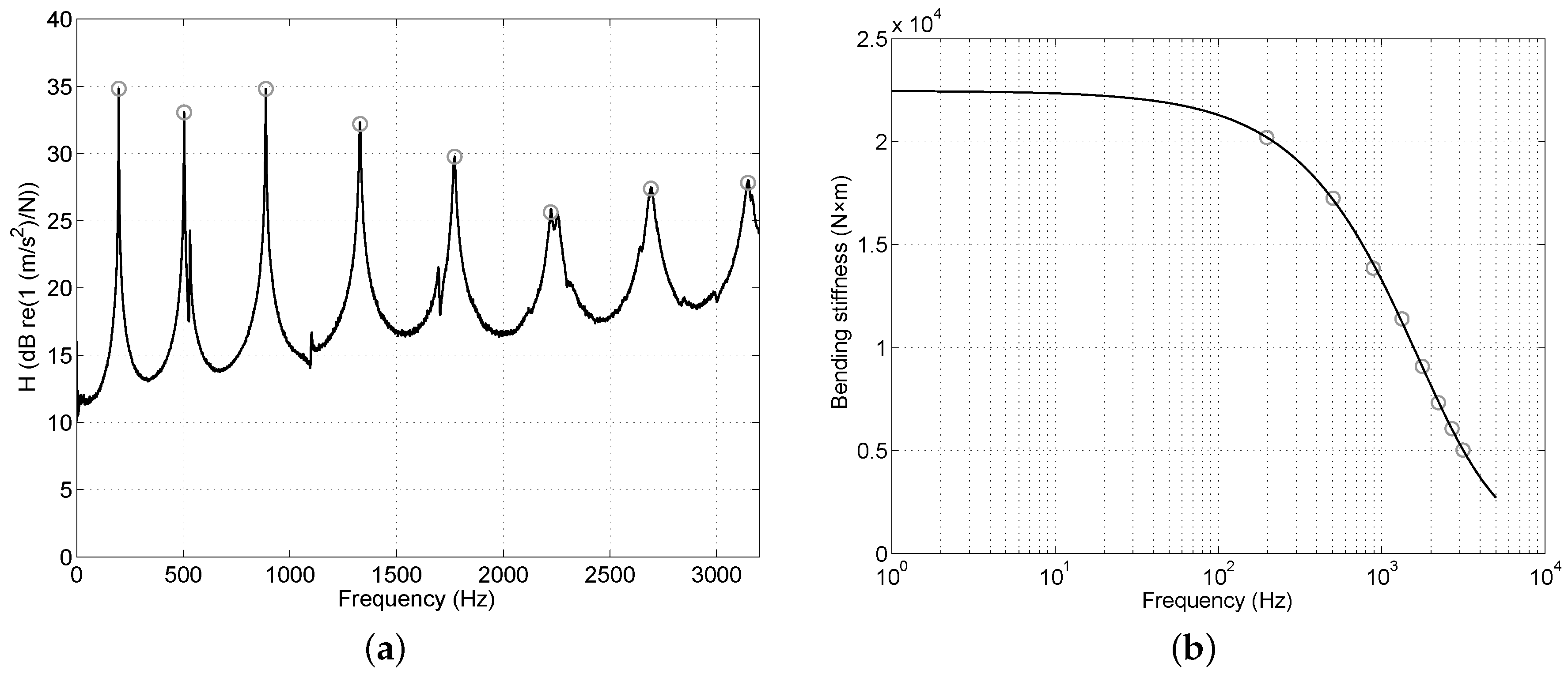
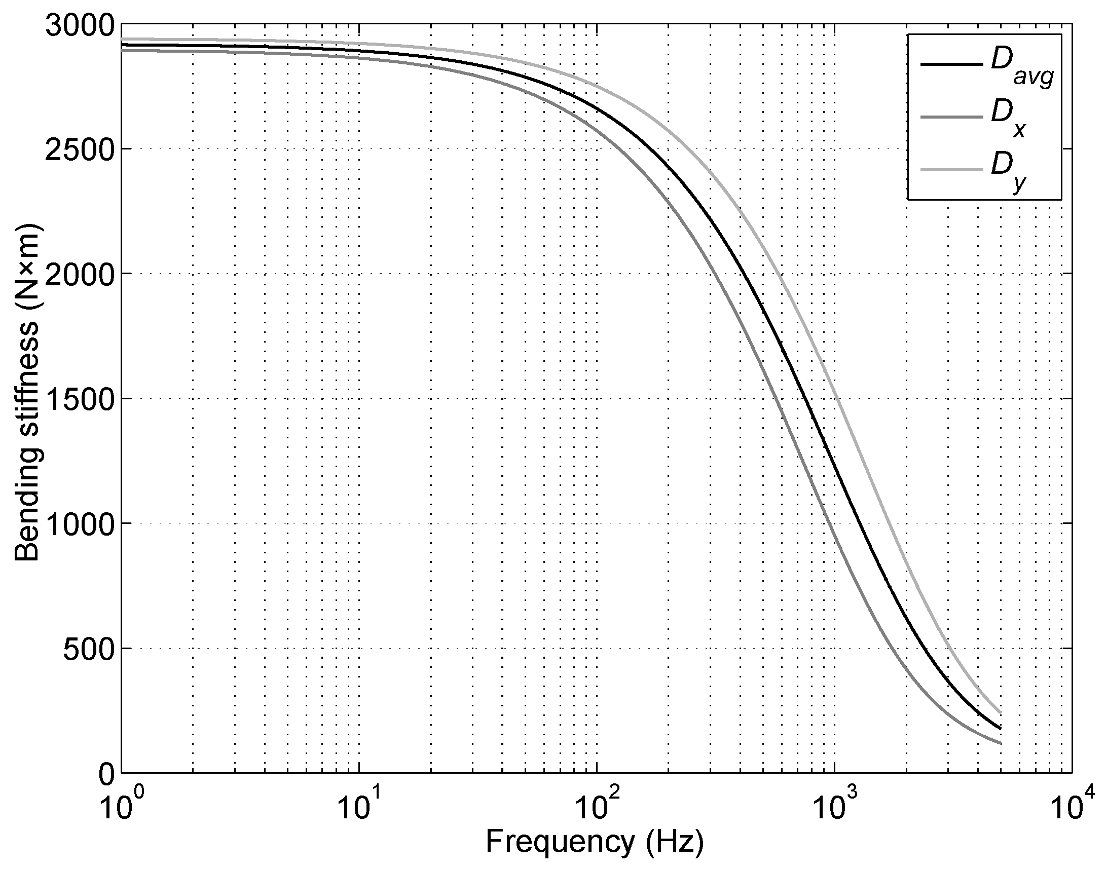
2.4. Determination of the Apparent Bending Stiffness

The frequency-dependent apparent bending stiffness $D_a^{\prime }$ introduced in Section 2.3 can be used in Equations (7)–(9) to obtain the sound transmission coefficient for a sandwich structure. For a finite Bernoulli–Euler beam of length L, the eigenfrequency $f_n$ of the bending wave equation for mode n can be expressed as:

$${\omega }_n=2\pi f_n=\frac{{\left(k_{n}L\right)}^2}{L^2}\sqrt{\frac{D^{\prime }}{m^{\prime }}}$$

(20)

where the eigenvalues $\left(k_{n}L\right)=a_n$ depend on the specific boundary conditions. If Equation (20) is rewritten as a function of the apparent bending stiffness, the following expression is obtained:

$$D_{x,n}^{\prime }=\frac{{\left(2\pi f_n\right)}^2{m}^{\prime }{L}^4}{a_n^4}.$$

(21)

Approximate values for $a_n$ are reported in

Table 1. Approximate $a_n$ value for increasing vibration modes, free-free boundary condition.

n	1	2	3	4	≥5
$a_n$	4.73	7.85	11.0	14.14	$n\pi +\pi /2$

for the free-free boundary condition [28].

The natural frequencies of a free-free beam can be measured in a relatively simple way. The beam can be suspended by strings, so to simulate free-free conditions, and excited at one end for example by an impedance hammer (Figure 5). The response of the beam can be measured by means of an accelerometer, whose mass must be negligible with respect to the mass of the tested specimen. The accelerometer has preferably to be mounted close to the opposite endpoint. The resulting signal, usually acceleration or velocity as a function of frequency, displays local maxima corresponding to the system eigenfrequencies, which can be used to obtain $D_{x,n}^{\prime }$ through Equation (21).

The A, B and C coefficients of Equation (18) can be estimated by applying the least-square (LS) method to the set of $\left(f_i,D_{x,i}^{\prime }\right)$ points obtained experimentally for each eigenfrequency, thus allowing the reconstruction of the apparent bending stiffness function along the entire frequency range of interest (usually 50 Hz–5 kHz). These coefficients can be computed once the eigenfrequencies and some simple geometric and mass data of the tested specimen are known. They can be used together with the definitions (19) to estimate some parameters that may be difficult to know in advance, such as the shear modulus $G_c$, the static bending stiffness of the beam $D_1^{\prime }$ and the bending stiffness of the laminates $D_2^{\prime }$.

Since many materials have an orthotropic behavior, in order to obtain information along the two main directions, two beams should be cut, in orthogonal directions, from a panel and tested separately. The composed bending stiffness can then be computed with a general formula that is applicable to different types of materials [29].

It is worth noting that a similar approach as the one developed for beams has been successfully applied to panels from which no beam could be cut, due to the large size of the products [30] or because they had been already installed [31]. In this case, the apparent bending stiffness function can be estimated from point mobility measurements.

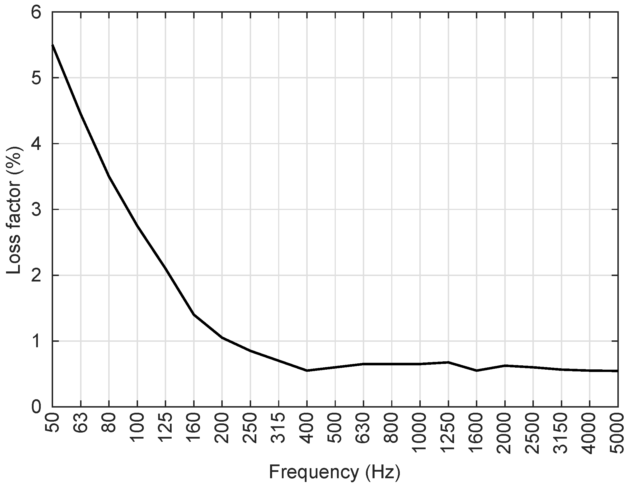
2.5. Losses in Solid Structures

Losses in solid structures are very important when the sound transmission loss has to be computed at and above the critical frequency. In some cases, increasing the losses can be an effective way to improve the sound transmission loss of a partition [32]. With the word ‘losses’, one typically indicates the conversion of vibrational energy into other forms, like thermal energy. The total losses are the sum of different contributions: internal losses, describing the inherent damping of the material; radiation losses, due to the coupling between the partition and the surrounding medium, which for lightweight structures are particularly relevant in the coincidence region; and boundary losses, induced by flanking transmission to the adjacent structures and significant in the low frequency range.

When comparing the predicted sound transmission loss to the experimental curves obtained in transmission suites, the total loss factor ${\eta }_{tot}$ must be considered to account for the actual behavior of the partition and measurement conditions. Studies to model the radiation component [33,34] and generic values of the internal loss factor [35] are available in the literature, but a complete theoretical determination of the loss factor is not possible to the present day. Experimental methods have been introduced for this purpose. By recording the decay of the vibration energy in a certain frequency band as a function of time, the loss factor can be estimated by applying the structural reverberation time technique, by means of Equation (22):

$${\eta }_{tot}=\frac{2.2}{f_{1/3}\times T_{60}},$$

(22)

where $f_{1/3}$ is the center-frequency of the one-third octave band of interest and $T_{60}$ is the time required for the vibration level to decay by 60 dB when the specimen is excited through an external force.

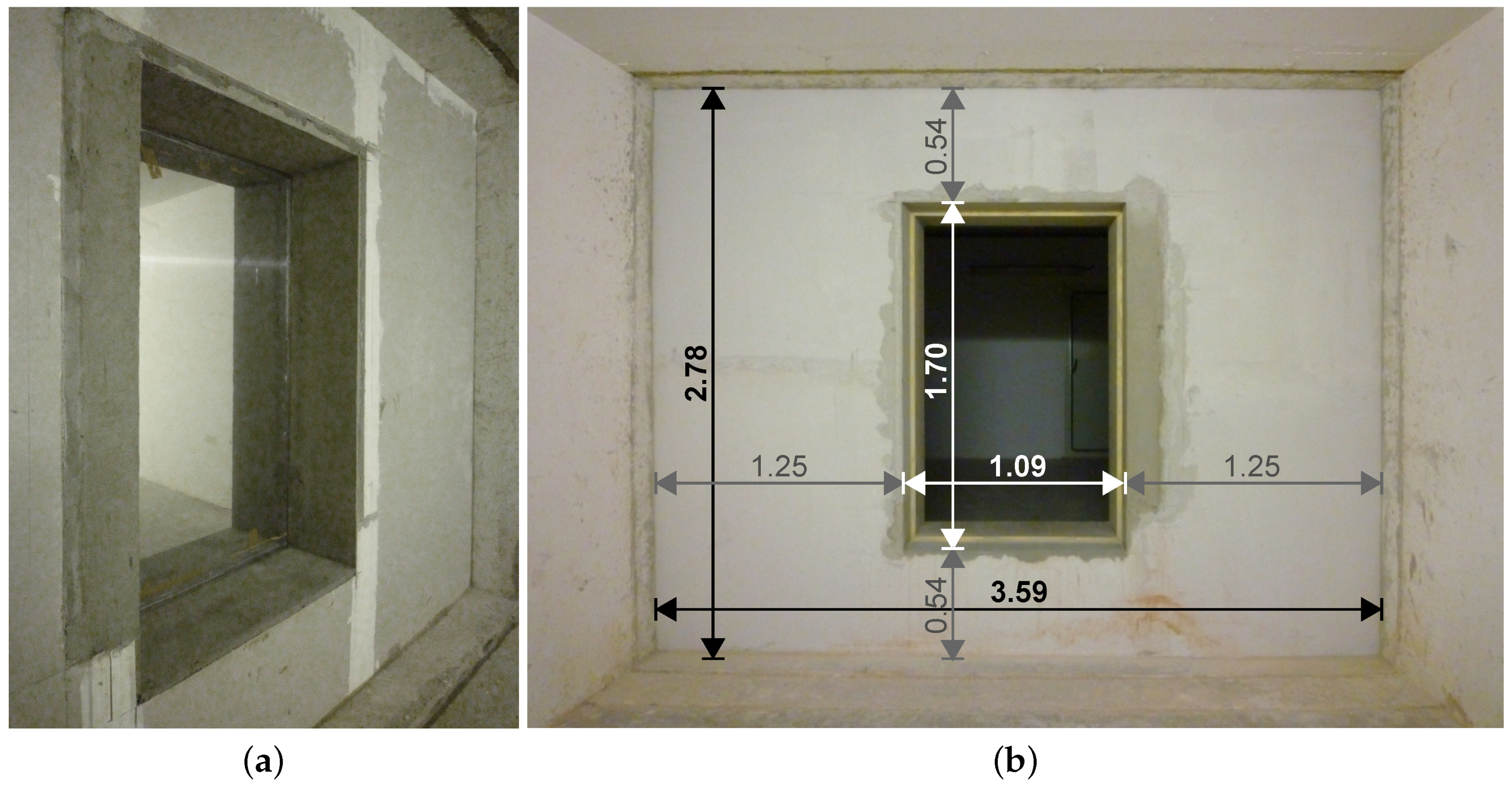
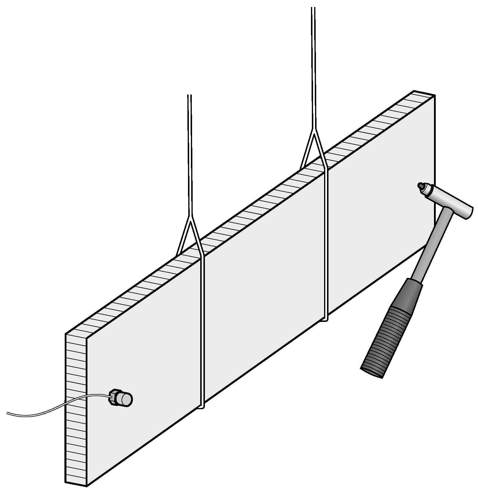
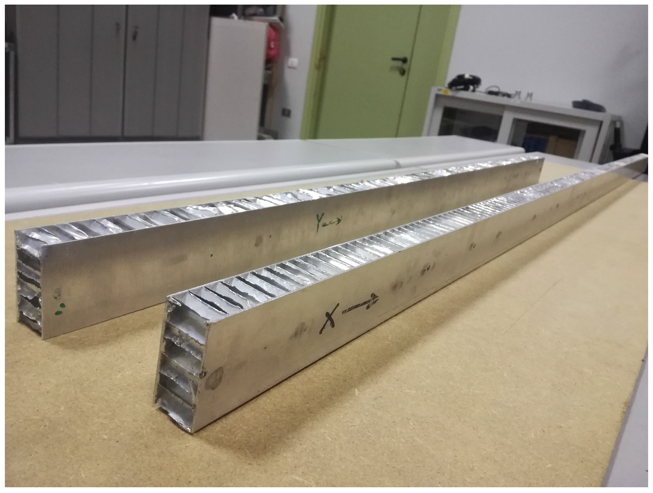
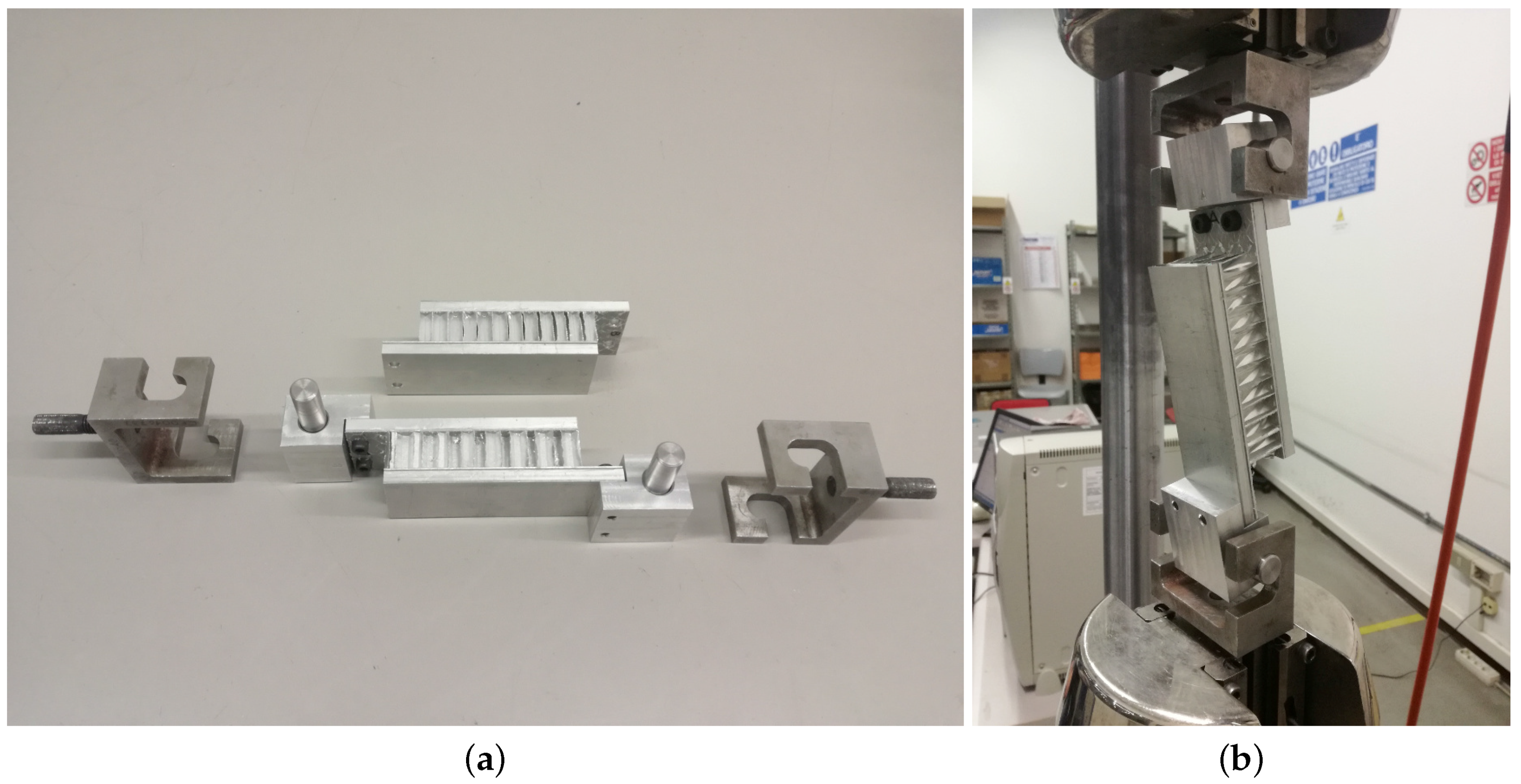
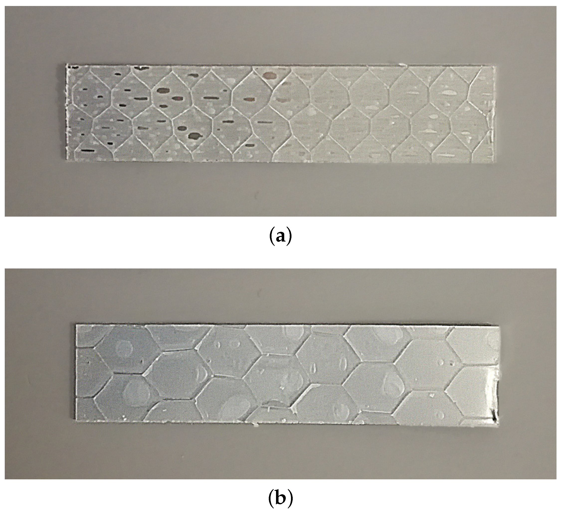
3. Materials and Methods

The material used for the tests features a 24-mm hexagonal aluminum honeycomb core sandwiched between two identical 1-mm aluminum laminates. Figure 6 shows a picture of the beams, while

Table 2. Characteristics of the beams used for natural frequency measurements.

Characteristics	Symbol	Units	x-Direction	y-Direction
Length	L	m	1.803	0.993
Core thickness	$h_c$	m	0.024
Laminate thickness	$h_l$	m	0.001
Width	b	m	0.050
Mass per unit area	$\mu$	kg m${}^{-2}$	6.72
Young’s modulus of the laminates	$E_l$	GPa	72
Cell size	-	in	3/8${}^{″}$
Core density	${\rho }_c$	kg m${}^{-3}$	46

summarizes the main geometrical and weight properties of the beams tested according to the method described in Section 2.4.

To derive the natural frequencies of beam test samples, the beams have been suspended through elastic strings (Figure 5). An accelerometer PCB Type 352A24 has been placed at one side of the beam, while the specimen has been hit using an impedance hammer PCB Type 086E80 with a plastic tip at the other end. The transducers have been connected to an OROS OR 36 analyzer. The software managing the analyzer can compute the frequency response function in real time. Once the eigenfrequencies are derived, the bending stiffness at a particular natural frequency can be computed by using Equation (21).

From the same panel the two beams have been cut from, a specimen had previously been obtained and tested in sound transmission suites. Figure 7 shows a picture of the panel ready to be tested according to the standard ISO 10140-2 [36]. The sound transmission loss has been determined on a 1.70 m × 1.09 m specimen. In order to avoid sound leakage through the sides of the specimens fit into the wall dividing the two hard rooms (Figure 7b), silicone has been used to seal the air gap between the wood frame of the opening and the plate. A second wooden frame has been used to close the perimeter of the panel and avoid lateral transmission through the edge. An omnidirectional sound source has been placed into the emitting room and a pink noise generated. The sound pressure levels in the emitting and receiving rooms have been measured by using an L&D 824 sound analyzer and subsequently space-averaged. The reverberation time has been measured using the interruption of a stationary pink noise. During the session, several structural reverberation time measurements have been performed in order to determine the loss factor. The signal has been recorded by using a PCB 352A24 accelerometer connected to an OROS OR 36 system. The panel has been hit close to the accelerometer position with a PCB impedance hammer Type 086C80 equipped with a nylon tip. The recorded signal has been further post-processed using Adobe^® Audition^® software and the Aurora plug-in [37]. The value of the structural reverberation time was then used to determine the total losses as an input in Equation (22).

No information about the shear modulus of the core was available at the time of this study since the manufacturer is no longer active on the market. For this reason, values relative to similar structures have been retrieved from datasheets of other manufacturers (see

Table 3. Core properties of commercial structures similar to the one at hand.

Manufacturer Model	Euro-Composites ECM 9.6-41	Alcore PAA-CORE™ 5052	Alucoat AluNID
Cell size	3/8${}^{″}$	3/8${}^{″}$	3/8${}^{″}$
${\rho }_c$ (kg m${}^{-3}$)	41	48	40
G (x-Direction) (MPa)	227	207	214
G (y-Direction) (MPa)	98	103	107

).

An attempt to experimentally measure the shear stress according to the ASTM C273/C273M-16 standard [38] has also been performed. The specimen is 0.05 m × 0.113 m and has been tested by using an Instron bench Model 8501. The stress-strain diagram has been recorder and the shear modulus computed with the following equation:

$$G_c\left(MPa\right)=\frac{s\left(\mathrm{N}/mm\right)\times h_c\left(mm\right)}{l\left(mm\right)\times b\left(mm\right)},$$

(23)

where s is the slope of the initial portion in the load-deflection curve, $h_c$ is the core thickness and l and b are the length and width of the specimen. Removing the leaves and testing only the core as the standard prescribes would have not been possible without damaging the material. For this reason, the sample featured the whole sandwich structure, and the clamps have been bonded directly to the external aluminum laminates by a professional adhesive. Pictures of the tested sample and of the experimental setup are shown in Figure 8.

4. Results and Discussion

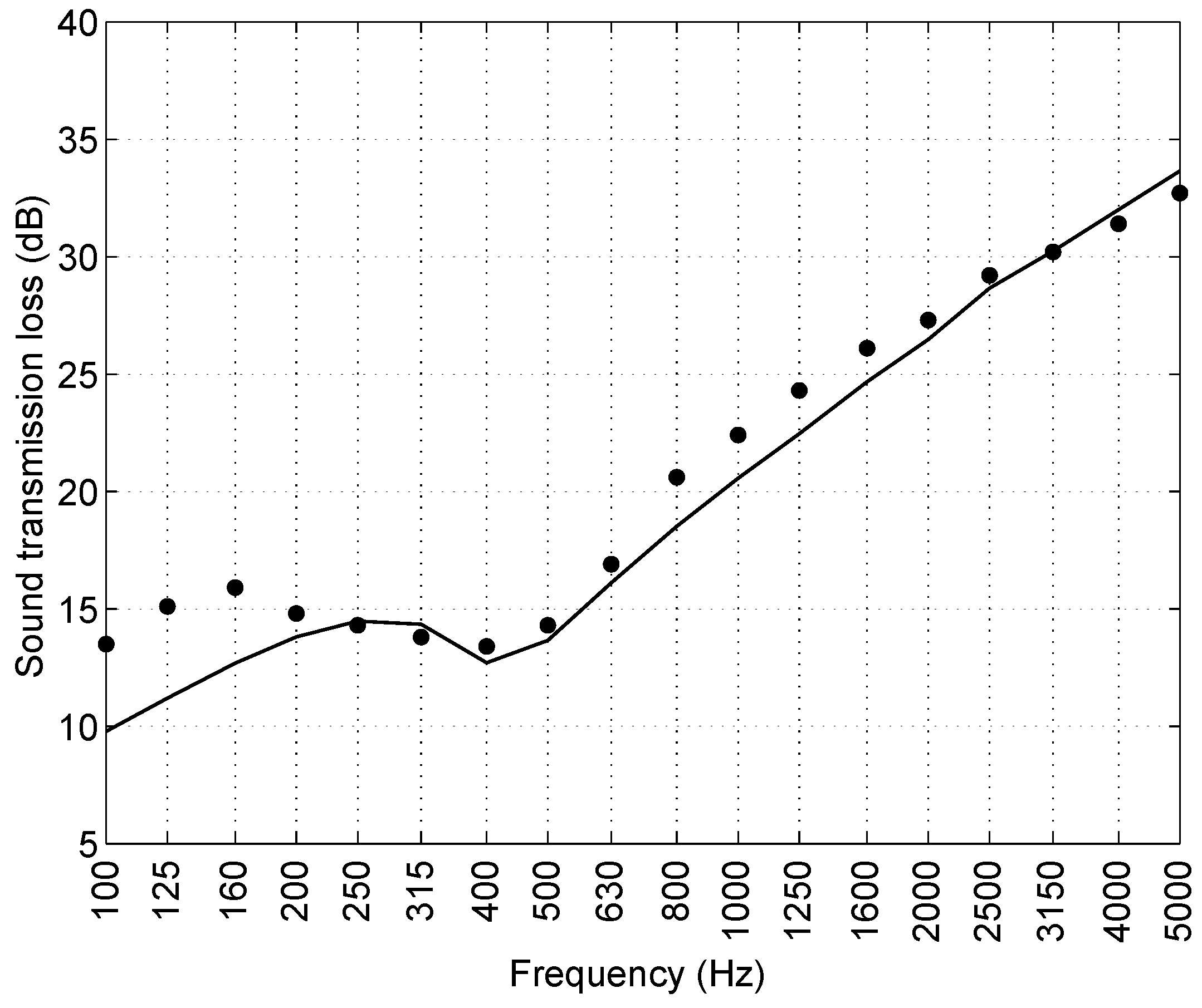
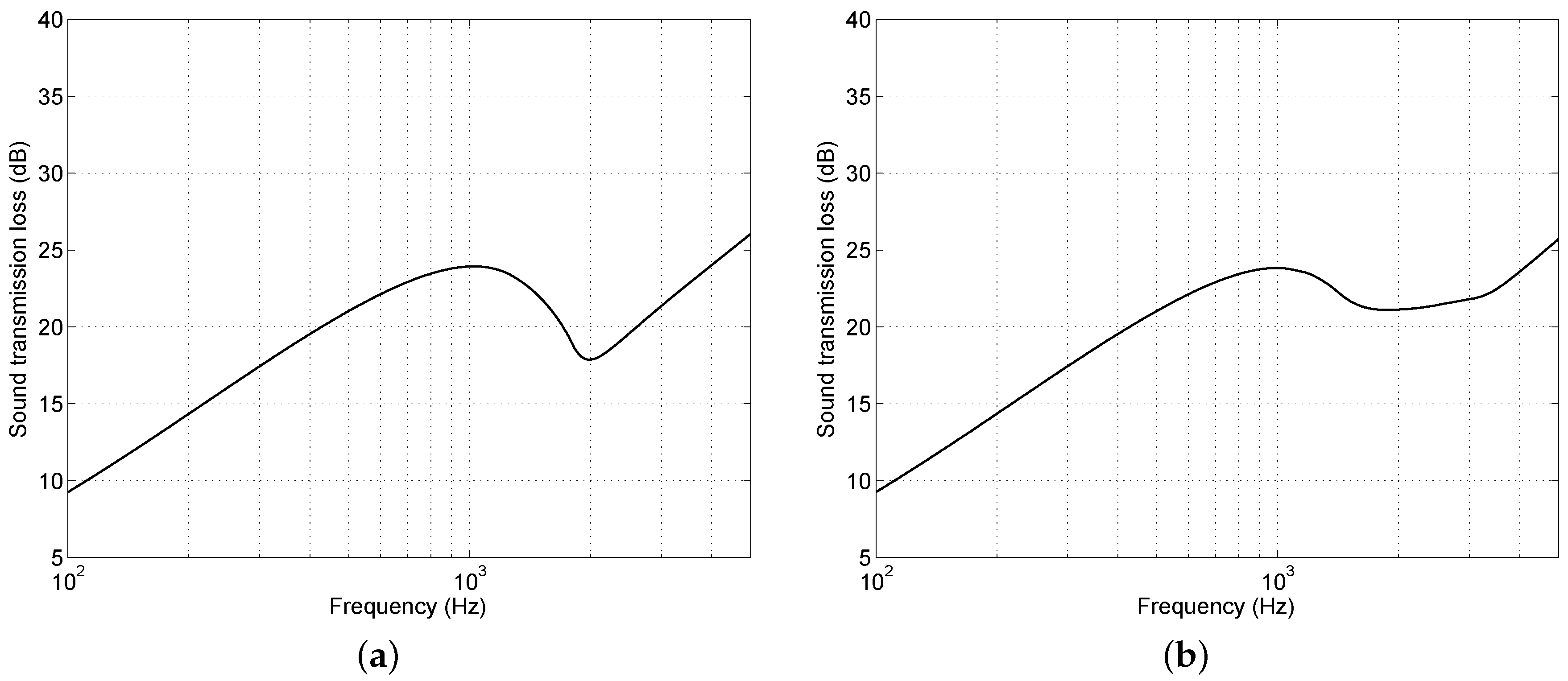
4.1. Sound Transmission Loss

Figure 9 shows the frequency response function measured on the beam cut in the x-direction. For each natural frequency (grey circles in Figure 9a), it is possible to compute the relevant bending stiffness points (grey circles in Figure 9b) as a function of frequency. The solid line in Figure 9b is the reconstructed apparent bending stiffness curve computed by applying the LS method to the experimental points.

The same procedure has been adopted for the beam cut in the y-direction (Figure 10).

The two apparent bending stiffness curves predicted in the x- and y-direction are compared and composed in Figure 11. The composed apparent bending stiffness $D_{avg}$ has been obtained from the average on the in-plane angle $\theta$ of the following function [29]:

$$D_a^{\prime }\left(\theta \right)={\left[{D_{a,x}^{\prime }}^{1/2}{cos}^2\left(\theta \right)+{D_{a,y}^{\prime }}^{1/2}{sin}^2\left(\theta \right)\right]}^2.$$

(24)

In computing the sound transmission coefficient ${\tau }_d$, the $\theta$-dependent bending stiffness function should be used and $\tau \left(\varphi ,\theta \right)$ should be integrated over the in-plane angle to obtain the sound transmission behavior of the whole structure.

The structural reverberation time technique has been used to measure the total loss factor necessary to calculate the sound transmission coefficient. The average loss factor has been computed by taking into account the results of five measurements carried out on randomly-distributed positions. The results of this procedure are reported in Figure 12. The loss factor varies from a maximum of 5.5% in the low frequency range to a minimum value of 0.5% for frequencies above 400 Hz.

The tested structure almost behaves like an isotropic material, and no significant difference has been found between computing ${\tau }_d$ from a single, averaged $D_{avg}$ function or a $\theta$-dependent $D_a^{\prime }\left(\theta \right)$ function. Either approach can therefore be used to derive the R index. Figure 13 reports the comparison between the predicted sound transmission loss (total loss factor as in Figure 12) and measurements in sound transmission suites. The agreement between predicted and measured curves is good above 200 Hz, while there is a discrepancy below this frequency due to the so-called ‘baffle effect’ [24]. The panel has a finite size and does not cover the entire surface of the wall dividing the two sound transmission suites. Since the sound transmission coefficient (Equation (8)) has been, in principle, derived for infinite panels, a correction may be required in the low frequency range. However, it is worth remarking how this simple technique proves to be extremely valid in predicting the location, extension and depth of the coincidence region at about 400 Hz.

For strongly-orthotropic structures, the coincidence effect is usually located in different frequency regions according to the in-plane angle. In this case, using a single ‘average’ apparent bending stiffness curve is not acceptable, and the $\theta$-dependent bending stiffness function should be used instead. As an example, Figure 14 reports the bending stiffness curves (x-direction, y-direction and averaged) obtained for a strongly-orthotropic honeycomb material with $h_l$ = 1 mm, $h_c$ = 8 mm and $\mu$ = 6.2 kg m${}^{-2}$, whose honeycomb footprint on the laminate can be observed in Figure 15b, as opposed to the almost isotropic structure tested in the rest of the work (Figure 15a).

Figure 16 shows the sound transmission loss computed by considering the structure as an isotropic panel with an equivalent, ‘average’ apparent bending stiffness (Figure 16a) or by computing a $\theta$-dependent apparent bending stiffness and integrating the sound transmission coefficient over the in-plane angle (Figure 16b). It can be observed that the latter approach allows one to account for the composition of the direction-dependent effects, resulting in a flatter, wider coincidence region.

4.2. Shear Modulus

Once the A, B and C coefficients are obtained, it is possible to use them to derive some properties of the structure, and in particular the shear modulus of the core, $G_c$.

Table 4. Comparison between the shear modulus of the core obtained from the B coefficient and estimated by product datasheets.

	Estimated	Product Datasheets (Average)
$G_{c,x}$ (MPa)	189	216
$G_{c,y}$ (MPa)	119	103

reports a comparison between the values estimated from the B coefficient and the average values obtained by product datasheets (see Table 3). An agreement around ±20% is found.

The shear modulus of the core can be a problematic parameter to determine experimentally, since standardized tests require the use of a strain-stress test bench and a complex setup. The measurements performed according to ASTM C273/C273M-16 provided results one order of magnitude lower than the expected values, the reasons being:

• a different sample aspect ratio (5:1) with respect to the standard prescriptions (12:1), an inevitable choice given the characteristics of the test bench;
• the presence of sandwich laminates and adhesive layers, which could not be removed without damaging the core;
• the use of aluminum clamps and plates, whereas the standard requires steel components, because of the technological limits of the available machining equipment.

All these elements contributed to return an evidently too low shear modulus. The proper arrangement of the measurement equipment and setup turned out to be essential to find reliable results, while a fair estimation based on the natural frequency method and wave propagation approach seems easier to obtain.

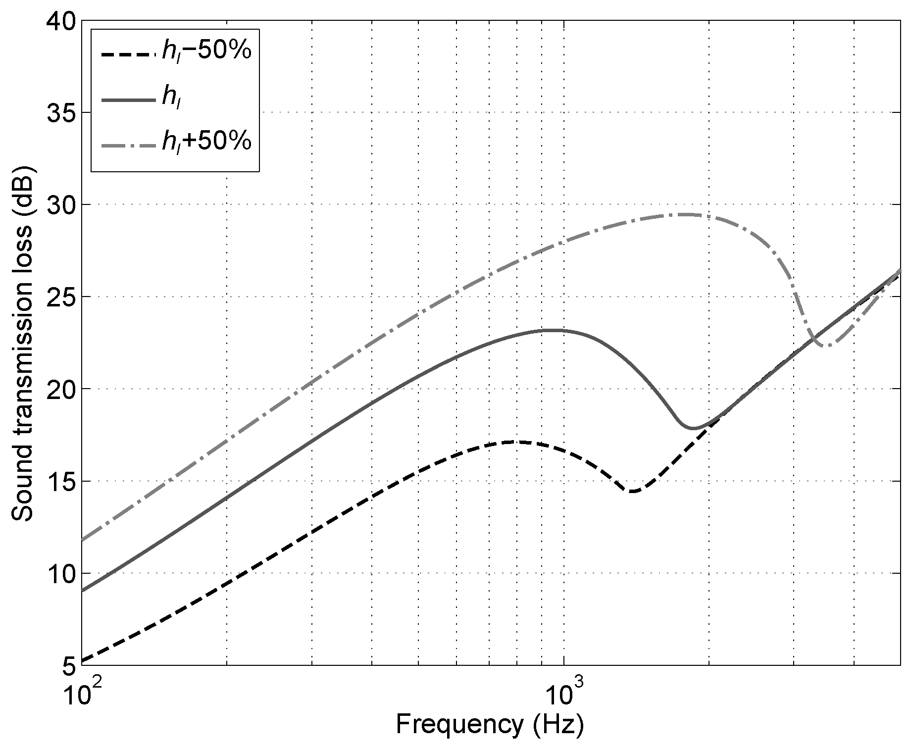
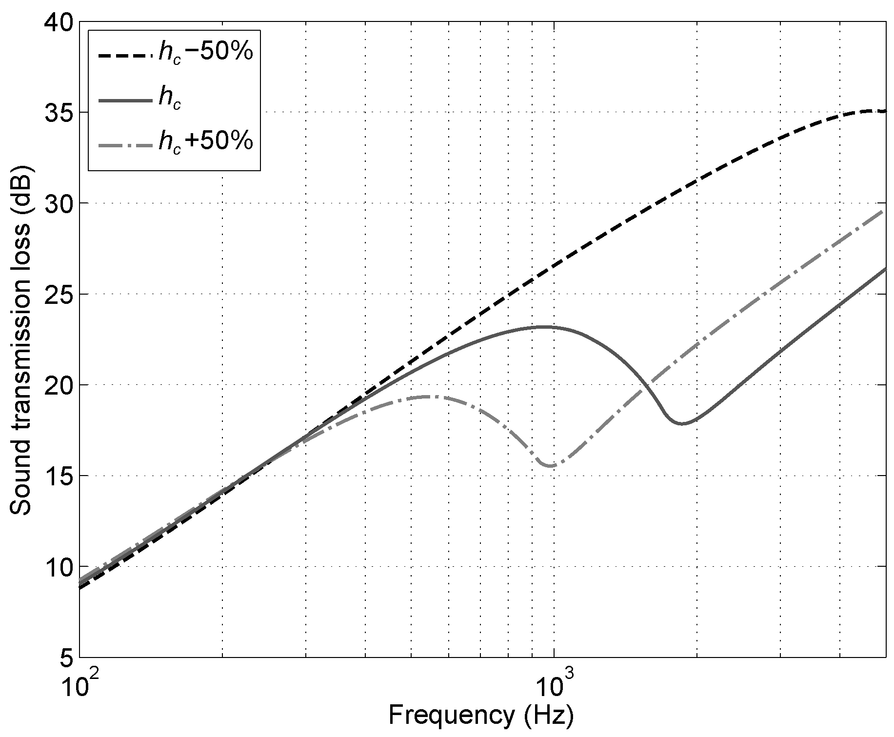
4.3. Parametric Study

The method proposed in this work can be used as a simple design tool to investigate different possible configurations for a new material. As an example, Figure 17, Figure 18 and Figure 19 separately show the influence of variations in the laminate thickness, core thickness and shear modulus on the sound transmission loss of the structure with respect to the existing configuration. It can be observed how this analysis can help in designing a material with the desired sound insulation or having the coincidence region in a specific frequency range. In particular:

• Figure 17: Increasing the laminate thickness increases the stiffness of the structure and its surface mass. As a result, the sound transmission loss below the critical frequency, following the mass law, increases, while the coincidence region moves to higher frequencies. No significant difference can be observed above $f_c$ due to the identical loss factor applied.
• Figure 18: An increase in the core thickness does not change the mass significantly since it is lightweight. Therefore, the mass-dominated region below $f_c$ does not change, either. The coincidence region moves to lower or higher frequencies depending on $D_a^{\prime }$, since $f_c\propto \sqrt{m^{\prime }/D_a^{\prime }}$.
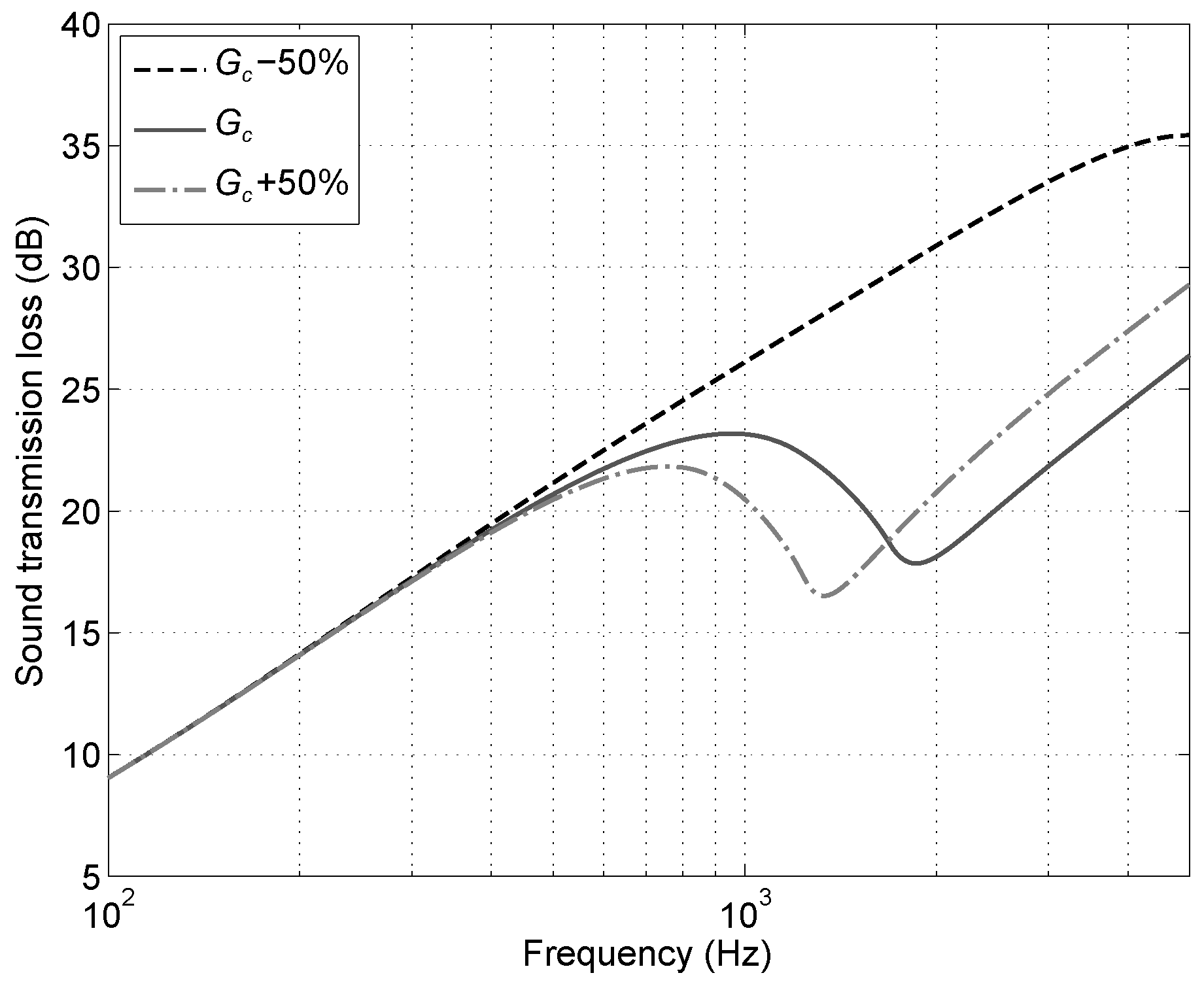
• Figure 19: Similar considerations to changing the core thickness also apply to changing the core shear modulus. The latter approach can be an interesting alternative in the case of weight or size constraints.

5. Conclusions

In this paper, a model based on the wave propagation approach has been applied to a honeycomb structure to derive several quantities: the apparent bending stiffness, the sound transmission loss and the shear modulus. To check the reliability of the method, the predicted sound transmission loss and shear modulus have been validated by comparison with experimental or literature data, finding good agreement. This technique proved to allow the estimation of many pieces of information about unconventional materials with limited experimental and computational effort. The method can be used to characterize a structure any time beam specimens are available, and such specimens satisfy the hypothesis of thin beams. In the design stage, the method provides useful information to evaluate different options and develop a material with the desired sound insulation properties.

References

1. U.S. Department of Transportation; Federal Aviation Administration. Advanced Composite Materials. In Aviation Maintenance Technician Handbook-Airframe, 2012 ed.; Aviation Supplies and Academics, Inc.: Newcastle, WA, USA, 2012; Volume 1. [Google Scholar]
2. Kumar, S.; Feng, L.; Orrenius, U. Predicting the sound transmission loss of honeycomb panels using the wave propagation approach. Acta Acust. United Acust. 2011, 97, 869–876. [Google Scholar] [CrossRef]
3. Crupi, V.; Epasto, G.; Guglielmino, E. Comparison of aluminum sandwiches for lightweight ship structures: Honeycomb vs. foam. Mar. Struct. 2013, 30, 74–96. [Google Scholar] [CrossRef]
4. Kee, P.; Thayamballi, A.; Sung, K. Strength characteristics of aluminum honeycomb sandwich panels. Thin-Walled Struct. 1999, 35, 205–231. [Google Scholar] [CrossRef]
5. Wu, Y.; Wang, F. Analysis for equivalent in-plane elastic parameters of the honeycomb core. Appl. Mech. Mater. 2014, 441, 84–90. [Google Scholar] [CrossRef]
6. Che, L.; Xu, G.D.; Zeng, T.; Cheng, S.; Zhou, X.W.; Yang, S.C. Compressive and shear characteristics of an octahedral stitched sandwich composite. Compos. Struct. 2014, 112, 179–187. [Google Scholar] [CrossRef]
7. Petrone, G.; D’Alessandro, V.; Franco, F.; De Rosa, S. Numerical and experimental investigations on the acoustic power radiated by Aluminium Foam Sandwich panels. Compos. Struct. 2014, 118, 170–177. [Google Scholar] [CrossRef]
8. Xu, X.; Jiang, Y.; Pueh, L. Multi-objective optimal design of sandwich panels using a genetic algorithm. Eng. Optim. 2017, 49, 1665–1684. [Google Scholar] [CrossRef]
9. Xu, X.M.; Jiang, Y.P.; Lee, H.P.; Chen, N. Sound insulation performance optimization of lightweight sandwich panels. J. Vibroeng. 2016, 18, 2574–2586. [Google Scholar] [CrossRef]
10. Griese, D.; Summers, J.; Thompson, L. The effect of honeycomb core geometry on the sound transmission performance of sandwich panels. J. Vib. Acoust. Trans. ASME 2015, 137. [Google Scholar] [CrossRef]
11. Grünewald, J.; Parlevliet, P.; Altstädt, V. Manufacturing of thermoplastic composite sandwich structures: A review of literature. J. Thermoplast. Compos. Mater. 2017, 30, 437–464. [Google Scholar] [CrossRef]
12. Krzyzak, A.; Mazur, M.; Gajewski, M.; Drozd, K.; Komorek, A.; Przybyłek, P. Sandwich Structured Composites for Aeronautics: Methods of Manufacturing Affecting Some Mechanical Properties. Int. J. Aerosp. Eng. 2016, 2016. [Google Scholar] [CrossRef]
13. Pourvais, Y.; Asgari, P.; Moradi, A.; Rahmani, O. Experimental and finite element analysis of higher order behavior of sandwich beams using digital projection moiré. Polym. Test. 2014, 38, 7–17. [Google Scholar] [CrossRef]
14. Li, P.; Liu, S.; Lu, Z. Experimental study on the performance of polyurethane-steel sandwich structure under debris flow. Appl. Sci. Switz. 2017, 7, 1018. [Google Scholar] [CrossRef]
15. Piana, E.; Marchesini, A.; Nilsson, A. Evaluation of different methods to predict the transmission loss of sandwich panels. In Proceedings of the 20th International Congress on Sound and Vibration, Bangkok, Thailand, 7–11 July 2013; International Institute of Acoustics and Vibrations: Auburn, AL, USA, 2013; Volume 4, pp. 3552–3559. [Google Scholar]
16. Visentin, C.; Prodi, N.; Bonfiglio, P.; Pompoli, R. On the prediction of transmission loss of honeycomb panels: Experimental measurements and numerical simulations. In Proceedings of the 7th Forum Acusticum, FA 2014, Krakow, Poland, 7–12 September 2014; European Acoustics Association: Madrid, Spain, 2014; Volume 2014-January, pp. 1–6. [Google Scholar]
17. Piana, E.; Marchesini, A. How to lower the noise level in the owner’s cabin of a yacht through the improvement of bulkhead and floor. In Proceedings of the 21st International Congress on Sound and Vibration, Beijing, China, 13–17 July 2014; International Institute of Acoustics and Vibrations: Auburn, AL, USA, 2014; Volume 5, pp. 3692–3699. [Google Scholar]
18. Davy, J.; Cowan, A.; Pearse, J.; Latimer, M. Predicting the sound insulation of lightweight sandwich panels. Build. Acoust. 2013, 20, 177–192. [Google Scholar] [CrossRef]
19. Scamoni, F.; Piana, E.; Scrosati, C. Experimental evaluation of the sound absorption and insulation of an innovative coating through different testing methods. Build. Acoust. 2017, 24, 173–191. [Google Scholar] [CrossRef]
20. Cremer, L.; Heckl, M.; Petersson, B.A.T. Structural Vibrations and Sound Radiation at Audio Frequencies, 3rd ed.; Springer: Berlin, Germany; New York, NY, USA, 2005. [Google Scholar]
21. Cremer, L. Theorie der Schalldämmung dünner Wände bei schrägem Einfall. Akustische Zeitschrift 1942, 7, 81–104. [Google Scholar]
22. Sharp, B.H. Prediction Methods for the Sound Transmission of Building Elements. Noise Control Eng. J. 1978, 11, 53–63. [Google Scholar] [CrossRef]
23. D’Alessandro, V.; Petrone, G.; Franco, F.; De Rosa, S. A review of the vibroacoustics of sandwich panels: Models and experiments. J. Sandw. Struct. Mater. 2013, 15, 541–582. [Google Scholar] [CrossRef]
24. Nilsson, A.; Liu, B. Vibro-Acoustics: 2, 2nd ed.; Springer: Berlin, Germany, 2015. [Google Scholar]
25. Nilsson, A. Wave propagation in and sound transmission through sandwich plates. J. Sound Vib. 1990, 138, 73–94. [Google Scholar] [CrossRef]
26. Nilsson, E.; Nilsson, A. Prediction and measurement of some dynamic properties of sandwich structures with honeycomb and foam cores. J. Sound Vib. 2002, 251, 409–430. [Google Scholar] [CrossRef]
27. Backström, D.; Nilsson, A. Modelling the vibration of sandwich beams using frequency-dependent parameters. J. Sound Vib. 2007, 300, 589–611. [Google Scholar] [CrossRef]
28. Blevins, R.D. Formulas for Natural Frequency and Mode Shape; Van Nostrand Reinhold Co.: New York, NY, USA, 1979. [Google Scholar]
29. Piana, E.; Milani, P.; Granzotto, N. Simple method to determine the transmission loss of gypsum panels. In Proceedings of the 21st International Congress on Sound and Vibration, Beijing, China, 13–17 July 2014; International Institute of Acoustics and Vibrations: Auburn, AL, USA, 2014; Volume 5, pp. 3700–3706. [Google Scholar]
30. Piana, E. A method for determining the sound reduction index of precast panels based on point mobility measurements. Appl. Acoust. 2016, 110, 72–80. [Google Scholar] [CrossRef]
31. Piana, E.; Petrogalli, C.; Solazzi, L. Dynamic and acoustic properties of a joisted floor. In Proceedings of the 6th International Conference on Simulation and Modeling Methodologies, Technologies and Applications, Lisbon, Portugal, 29–31 July 2016; Obaidat, M.S., Merkuryev, Y., Oren, T., Eds.; SciTePress: Setúbal, Portugal, 2016; pp. 277–282. [Google Scholar]
32. Hopkins, C. Sound Insulation, 1st ed.; Butterworth-Heinemann: Amsterdam, The Netherlands, 2007. [Google Scholar]
33. Maidanik, G. Response of Ribbed Panels to Reverberant Acoustic Fields. J. Acoust. Soc. Am. 1962, 34, 809–826. [Google Scholar] [CrossRef]
34. Leppington, F.; Broadbent, E.; Heron, K. The acoustic radiation efficiency of rectangular panels. Proc. R. Soc. Lon. Ser. A Math. Phys. Sci. 1982, 382, 245–271. [Google Scholar] [CrossRef]
35. Bies, D.A.; Hansen, C.H. Engineering Noise Control: Theory and Practice, 4th ed.; CRC Press: London, UK; New York, NY, USA, 2009. [Google Scholar]
36. International Organization for Standardization. ISO 10140-2:2010–Acoustics–Laboratory Measurement Of Sound Insulation of Building Elements–Part 2: Measurement of Airborne Sound Insulation; ISO: Geneva, Switzerland, 2010. [Google Scholar]
37. Farina, A. AURORA Plug-ins. Available online: http://pcfarina.eng.unipr.it/Aurora_XP/index.htm (accessed on 25 November 2017).
38. American Society for Testing and Materials. ASTM C273/C273M-16–Standard Test Method for Shear Properties of Sandwich Core Materials; ASTM: West Conshohocken, PA, USA, 2016. [Google Scholar]
Figure 1. Breakdown of the incident power: (1) into the main components: (2) reflected; (3) transmitted to adjacent structures; (4) dissipated; (5) transmitted across the partition.
Applsci 08 00045 g001
Figure 2. Bending of a beam in the plane x , y .
Applsci 08 00045 g002
Figure 3. Sandwich beam: schematic (a) and displacement (b).
Applsci 08 00045 g003
Figure 4. Example of wavenumbers obtained from Equation (14) (beam data source: [27], except laminate thickness, assumed 1 mm for both leaves).
Applsci 08 00045 g004
Figure 5. Measurement of free-free natural frequencies with impedance hammer and accelerometer.
Applsci 08 00045 g005
Figure 6. Beams used for natural frequency measurements (x- and y-direction).
Applsci 08 00045 g006
Figure 7. (a) Panel mounted in the opening of the sound transmission suites; (b) dimensions of the opening and of the dividing wall.
Applsci 08 00045 g007
Figure 8. Experimental measurement of the core shear modulus: (a) specimen and clamping system; (b) test setup.
Applsci 08 00045 g008
Figure 9. x-direction. (a) Measured transfer function and natural frequencies (grey circles); (b) bending stiffness from measured natural frequencies (grey circles) and approximated by the LS method (solid line).
Applsci 08 00045 g009
Figure 10. y-direction. (a) Measured transfer function and natural frequencies (grey circles); (b) bending stiffness from measured natural frequencies (grey circles) and approximated by the LS method (solid line).
Applsci 08 00045 g010
Figure 11. Comparison of bending stiffness curves in the x- and y-direction and their composition ( D a v g ).
Applsci 08 00045 g011
Figure 12. Loss factor measured with the structural reverberation time technique.
Applsci 08 00045 g012
Figure 13. Sound transmission loss predicted (solid line) vs. measured in sound transmission suites (bullets).
Applsci 08 00045 g013
Figure 14. Apparent bending stiffness (x-direction, y-direction and composition) for a strongly-orthotropic structure.
Applsci 08 00045 g014
Figure 15. Honeycomb footprint on the laminates: (a) slightly-orthotropic material (present work); (b) strongly-orthotropic material.
Applsci 08 00045 g015
Figure 16. Sound transmission loss for the honeycomb in Figure 15b, predicted assuming an isotropic structure with ‘average’ bending stiffness D a v g (a) and assuming an orthotropic structure with θ -dependent apparent bending stiffness D a θ (b).
Applsci 08 00045 g016
Figure 17. Sound transmission loss variation with varying laminate thickness, h l .
Applsci 08 00045 g017
Figure 18. Sound transmission loss variation with varying core thickness, h l .
Applsci 08 00045 g018
Figure 19. Sound transmission loss variation with varying core shear modulus, G c .
Applsci 08 00045 g019