Swarming Behavior Emerging from the Uptake–Kinetics Feedback Control in a Plant-Root-Inspired Robot


Center for Micro-Biorobotics, Istituto Italiano di Tecnologia, 56025 Pontedera, Italy
*
Authors to whom correspondence should be addressed.
Appl. Sci. 2018, 8(1), 47; https://doi.org/10.3390/app8010047
Submission received: 15 November 2017
/
Revised: 12 December 2017
/
Accepted: 26 December 2017
/
Published: 1 January 2018
(This article belongs to the Special Issue Bio-Inspired Robotics)
Abstract
:This paper presents a plant root behavior-based approach to defining the control architecture of a plant-root-inspired robot, which is composed of three root-agents for nutrient uptake and one shoot-agent for nutrient redistribution. By taking inspiration and extracting key principles from the uptake of nutrient, movements and communication strategies adopted by plant roots, we developed an uptake–kinetics feedback control for the robotic roots. Exploiting the proposed control, each root is able to regulate the growth direction, towards the nutrients that are most needed, and to adjust nutrient uptake, by decreasing the absorption rate of the most plentiful one. Results from computer simulations and implementation of the proposed control on the robotic platform, Plantoid, demonstrate an emergent swarming behavior aimed at optimizing the internal equilibrium among nutrients through the self-organization of the roots. Plant wellness is improved by dynamically adjusting nutrients priorities only according to local information without the need of a centralized unit delegated for wellness monitoring and task allocation among the agents. Thus, the root-agents can ideally and autonomously grow at the best speed, exploiting nutrient distribution and improving performance, in terms of exploration capabilities and exploitation of resources, with respect to the tropism-inspired control previously proposed by the same authors.
1. Introduction
A decentralized control system is a system in which the components act on the basis of local information when accomplishing global tasks. In such systems, the collaborative behavior emerges from independent local decisions without the need for centralized processing [1]. This definition is intrinsically linked to the idea of self-organization. Many natural systems have been studied in terms of their ability to perform complex tasks without a centralized control but due to simple rules followed by many distributed agents with communication capabilities [2]. Well-known examples include ant colonies that are able to accomplish foraging tasks by following pheromone trails [3], or honeybees that indicate the direction of the nectar source by dancing [4]. However, systems that also have no nervous system are considered, such as bacteria that organize themselves in order to maximize nutrient availability [5].
The analysis of these behaviors has inspired routing algorithms [6], load balance problem solutions [7], ant colony optimization [8] or particle swarm optimization [9] algorithms. This approach typically provides a scalable and robust solution to large-scale complex problems. It has also opened the door to a relatively new discipline, called swarm robotics, which applies swarm intelligence principles to robotics [10]. Collaborative exploration specifically in unstructured environments such as disasters or dangerous areas is a particularly important application of this discipline.
Like animals, plants also need to explore the environment for foraging purposes. They actively interact with the environment perceiving, for instance, the presence of obstacles and adjusting their growth when mechanically stimulated [11,12]. Moreover, they need to optimize their energy due to the uncertainty of nutrient availability. Specifically, production, mobilization and allocation among the tissues of photosynthesis products (e.g., carbon and sugars), that regulate plant growth and development, are highly affected by sugar and hormone signals in response to environmental cues [13,14,15]; in addition, nutrient uptake and usage are regulated according to the availability of the nutrient [16]. However, unlike animals, plant locomotion is irreversible, since it takes place through organ growth, which suggests that plants should focus more on decision-making activities compared to animals.
Plants have been already taken as source of inspiration in engineering [17,18,19], and they have been also explored for optimization algorithms [20]. Macro-rules for the design of metaheuristics have been extracted for instance from pollination processes [21], the colonization of invasive weeds [22] or strawberry plant propagation strategies [23]. Plant roots have also been considered, in particular, their distribution in searching for optimal soil, water, and fertilizer conditions. Specifically, Qi et al. [24] proposed the Root Mass Optimization Algorithm (RMO) where the search for optimality is driven by operators inspired by the concepts of growth and branching, and the search evolves through generations of roots, as with a classical genetic algorithm. Roots, which represent different initialization points in the search domain, can grow in conditions of optimal soil impedance, water, and fertilization. This optimal condition is monitored by a fitness function. In addition, roots can decide to generate a branch with a random probability in a random position; each root is then evaluated and the best are selected for the next generation. Similarly, Zhang et al. [25] proposed the Root Growth Algorithm (RGA) based on root branching and root hair growth operators. In this case, the length and distance of hairs and roots are also important in obtaining wider spatial distribution and increasing the diversity of fitness values.
However, to our knowledge, in the robotic community, plants have not yet been explored as swarm intelligent systems, while at the same time extensively analyzing plant root behavior.
In the field of robotics, in a previous paper, we analyzed plant root behavior for the implementation of a plant-inspired control [26]. The previous control was inspired by the tropic responses of plant roots, e.g., attraction to water, attraction to gravity, attraction to an optimal defined temperature, repulsion to obstacles. From the observation of tropisms, we developed a stimulus-oriented control. The direction of growth or bending was defined by combining the preferential direction obtained for each stimulus. Each stimulus had a fixed priority to amplify the attraction or repulsion towards or away from that stimulus, and, by vectorization, we defined the preferred direction of growth or bending. However, at this stage, the chemical signals were neglected with a consequent disregard of the nutrient uptake mechanism and the regulation of internal needs. The robotic roots operated independently on the basis of local perception, without an internal memory and with no inter-agent communication.
This paper presents a plant root behavior-based approach for defining the control architecture of a plant-root-inspired robot. Specifically, we looked at the movements, communication channels and uptake mechanism used by plant roots to explore and exploit the environment for the entire plant survival. We demonstrate that taking inspiration from plants can lead to the extraction of new technologies and control principles that are relevant in robotics as well as in other fields (e.g., optimization problems, traffic management, marketing strategies, etc.), in the same way as ethology did. At the same time, this approach can improve the knowledge on plant behavior by extending the analysis of internal processes.
In this work, we aim to verify the hypothesis that plant roots can be considered as simple agents working as a swarm in order to ensure plant survival, although still acting independently on the basis of local information and perception. With respect to our previous plant-inspired control [26], in this paper, we introduce local memory, inter-agent communication and the dynamic evolution of nutrient priorities.
Section 2 provides an extensive explanation of the biological aspects characterizing plant root behavior from which the main properties for control are extracted (Section 2.1) and from which the plant wellness problem is formalized (Section 2.2). These features are then implemented as a control strategy for a robotic platform, the Plantoid [26], which mimics the key movements of plant roots, i.e., directional bending of the apical part of the root. The robotic system and the simulated environment used for validation are briefly introduced in Section 2.3, followed by a detailed presentation of the implemented control (Section 2.4) and the experiments performed to validate the hypothesis (Section 2.5). Results of simulations and of the experiment performed on the robot are presented in Section 3, and discussed in Section 4.
2. Materials and Methods
2.1. Clues from Plants
2.1.1. Uptake–Kinetics
As plants are sessile organisms, they have to develop a series of strategies for survival. The ability to adapt morphological and physiological properties to environmental stimuli is called plasticity and has enabled plants to explore and exploit the environment [27]. The role of roots is to supply nutrients to the whole plant. In order to maximize the probability of success, they have developed several strategies for nutrient exploitation, e.g., increase in root hairs, growth of lateral roots in patches of soil that is nutrient rich (morphological plasticity) or increasing the nutrient uptake rate (physiological plasticity) in conditions of nutrient deficiency [28].
In soil, nutrients are not always present and distributed in such a way to satisfy the requirements of plants for optimal growth [29]; indeed, plant growth is limited by their availability, quantity, and ratio [30]. Ion charges in plants also need to maintain a balance for the correct evolution of processes such as protein synthesis or ion transportation through the membranes. Experiments evaluating the interaction among ions show in fact that the uptake of Na+ and K+ changes according to the presence of calcium in the medium or processes such as the synthesis of organic acids are altered by excessive cation or anion uptake [31]. These observations suggest that the internal concentrations of nutrients in plants need to maintain an equilibrium to prevent process alterations. Various characteristic indices and requirements among macronutrients have also been established [32].
There is thus the first fundamental property of plant behavior:
Property 1:
Plant growth is driven more by maintaining a balance of the internal nutrient concentrations rather than by collecting the closest and most available nutrient in the soil.
The consequence of Property 1 is the selectivity of ion uptake. Uptake rates have been analyzed in both lower and higher plants by comparing the accumulation of nutrients in roots with the concentration remaining in the external solution. Results have shown that ratios among these two quantities differ for each observed nutrient [31], and thus confirm the selective characteristic of nutrient absorption by plants.
Nutrient uptake is known to work as a function of the nutrient concentration in soil (at least up to a limiting threshold) with the saturation kinetics mechanism, which is described by the Michaelis–Menten equation [33], and defines the uptake rate, or absorption velocity, as:
In Equation (1), identifies the capacity factor, maximal rate of absorption, which is approached asymptotically when the ion concentration in the medium increases. represents the concentration with half of the maximal rate of absorption and is the concentration perceived. It has been shown that the parameters of the uptake–kinetics ( and ) are strongly influenced by the internal concentration status of the plant. For instance, in both Zea mays (corn) and soybean, it has been shown that with an increasing concentration of phosphorus in plants, both parameters decrease linearly ( more rapidly than ) [34]. The same behavior has been observed in barley roots when the internal nitrate availability increases [35]. This adjustment of and suggests a second property:
Property 2:
A feedback control modifies the uptake rate of a nutrient according to its internal state in plants.
2.1.2. Tropisms
Another kind of plasticity shown by plants is the directional response to environmental stimuli, which can be attractive or repulsive (tropism); for instance, gravity is an attractive stimulus in roots, inducing them to bend towards the gravity vector (gravitropism). With thermotropism, temperature has been shown to be attractive (repulsive) when a low (high) threshold temperature is reached [36]. And directed responses towards increasing concentrations of moisture with hydrotropism [37], or towards attractive chemicals in chemotropism [38] (or away from negative chemicals [39]) have also been observed. These and many other tropisms (thigmotropism, phototropism, magnetotropism, etc.) interact with each other, thus leading to a unified directional response [40]. For instance, the interaction between gravitropism and mechanical stimulation has been analyzed observing a modulation of the response to gravity under mechanical stress [41]; analogously, the interaction among gravitropism and hydrotropism showed a reduced response to gravity in the presence of moister gradients [42].
The above observations can be summarized in three main properties of plant root behavior:
Property 3:
Roots show directional responses towards or away from a stimulus;
Property 4:
The directional response is probably induced by the perception of a gradient;
Property 5:
Tropic responses are combined to obtain a single directional response.
2.1.3. Plant Intra-Communication and Local Storage
The sharing of minerals and other substances between roots and shoot is possible in plants thanks to the internal vascular system, which is composed of two channels, called the xylem and phloem (Figure 1). The xylem is the central vessel that runs along the whole structure and represents a direct omnidirectional connection from roots to shoot. Here, water and nutrients are transported by bulk flow, exploiting water pressure, to the aerial parts of the plants. On the other hand, the phloem is a slower connection channel, with an osmotic mechanism, enabling substances to be diffused from source to sink. In this channel, elements move from an area with a high concentration (source) to an area with a lower concentration (sink). In fact, the direction of transport is defined by the nutritional requirements of the different plant organs or tissues, ensuring nutrient cycling and a fair redistribution between shoot and roots. It can thus be considered as an important communication channel of the internal nutritional status [31], e.g., if a required nutrient is not delivered to the sink, it is highly probable that that nutrient is not available.
Once mineral nutrients in the soil reach the root surface and are absorbed by cells, they can (I) be immediately used for local processes (e.g., protein synthesis), (II) sent to the shoot through the xylem or (III) stored in vacuoles, which are cell components that work as pools for substances that need to be readily provided to cell processes [43]. When the request from the shoot is high, nutrients are rapidly pumped up (alternative II), and then redistributed towards the requesting sinks.
Plants thus also have the following three properties:
Property 6:
There is a fast and direct highway where nutrients are transported immediately from roots to shoot;
Property 7:
Nutrients are distributed among requesting organs according to the strength of their requests;
Property 8:
Root tissues and cell vacuoles are local memories storing information on nutrient status.
In fact, regulation of the uptake rate has been correlated to the mineral nutrients stored in vacuoles [44].
2.2. Plant Wellness Problem
The eight properties outlined in Section 2.1 indicate that the interest of the entire plant is to collect nutrients, thus preserving optimal ratios in order not to compromise the correct functioning of internal processes. To confirm this theory, the demand of nutrients in plants was found to reflect specific ratios between nutrients (i.e., N:P and K:P both equal to 10) [45]. We can thus formalize the plant's interest in minimizing the imbalance () among nutrients during its life (for every instant of time ):
with the imbalance defined as:
where represents the set of nutrients and represents the ratio between nutrient and , where is a nutrient chosen as reference among all. is the concentration of nutrient in the entire plant at a certain instant of time (). The concentration in the plant of a single nutrient in a certain instant of time can then be obtained by:
where is the number of roots in the apparatus, is the uptake of nutrient from root at time and is the consumption of nutrient from root at time . In (4), for this work, only uptake and consumption actuated by the root apparatus are considered, neglecting photosynthesis and other transformation processes actuated in the shoot.
2.3. Robotic Architecture, Simulated Environment and Sensing
Root-inspired behavior was implemented first in a simulation and then in a robotic platform called Plantoid, which is a plant-inspired robot with a root apparatus where the robotic roots mimic the bending movements of plant roots thanks to the actuation of three soft springs that can elongate differentially [26]. Each root is endowed with perception capabilities by embedding an accelerometer, to detect gravity, three commercial temperature sensors, placed at 120° from each other, and customized humidity and tactile sensors (for details on the design and sensors, see [26]).
The overall system (Figure 1) can be considered as a multi-agent system with two types of agents: a shoot agent, grouping all aerial elements (trunk, branches and leaves), dedicated in this implementation only to the collection and redistribution of nutrients, plus three root agents that search for and collect nutrients. Root and shoot agents, in the following also only called roots and shoot unless ambiguous, each have their local memory for nutrient storage with a maximal capacity (with variable name storeCapacity) for each nutrient (Property 8). Roots have a direct communication with the shoot in both directions to simulate the xylem channel (from roots to shoot) and phloem channel (bidirectionality).
With the three soft spring robotic roots, it is possible to visualize the directional response by bending the root (Supplementary Video S1). While growth is simulated on a virtual environment created in MATLAB (R2016b, The Mathworks, Natick, MA, USA) and containing three roots where only the skeleton is visible. The simulated environment is used to plot tip positions (the apical part is at the beginning oriented downwards), the historical path (previous positions of the point at the back of the tip) and to provide a chemical stimulation to the robotic tips. Roots are stimulated with gravity and chemical stimuli. On the robot, temperature sensors are used instead of chemical sensors, thus the gradient of a nutrient is simulated with a gradient of temperature, while the other two nutrients are provided with the virtual environment to the robot. Consequently, chemical receptors on the simulated roots are localized at the same positions as temperature sensors present in the robotic root. In fact, there is a receptive site for nitrate (N), for potassium (K) and for phosphorus (P) every 120° along the circumference of the tip.
The environment simulates static gradients of the three selected nutrients (Figure 2), drawn with a Gaussian function:
with Gaussian root mean square width, maximal concentration and central location of nutrient in the soil.
The proof of concept works best with a simplified system so several assumptions were made. For instance, it is assumed that all nutrients are highly requested by the shoot to force the immediate sending of the total amount from roots to shoot (using Property 6—alternative II in Section 2.1.3). It is assumed that there is always enough water potential to pump ions in the xylem channel, and to always have a constant optimal temperature in order to consider the influence of this factor to be negligible on the uptake–kinetics parameters. In addition, only the interaction between gravity and attractive chemicals are considered here.
The aerial part in this case only works as a gateway, collecting and redistributing the absorbed nutrients. This means that processes such as photosynthesis and nutrient transformation are not modeled. Consequently, energy production, redistribution, and consumption are not considered here.
Taking this simplification into account, to prevent a rapid filling of local storages, a consumption factor was introduced to decrease the root local memory, which should be in the future related to energy consumption. All three nutrients are decreased with an amount equal to the minimum nutrient stored minus a constant threshold.
2.4. Uptake–Kinetics Feedback Control
At each time step, each root takes a decision independently from the other and with only the knowledge of its internal state and environmental perception. Therefore, each robotic root is an autonomous agent that repeatedly performs steps in the following order:
- Update of internal state and uptake–kinetics parameters;
- Perception of the environment;
- Uptake of nutrients;
- Nutrients sent to shoot;
- Evaluation of growing direction;
- Growth.
As the shoot is a collector and distributor of nutrients (satisfying Property 7), when it receives all the nutrients from each agent, it sends an amount of nutrients back in proportion to the request received from the root. In fact, together with the uptake, each root also makes a request to the shoot for each nutrient that corresponds to the free internal memory. The request is expressed by the root as a percentage of free memory over the storeCapacity.
The feedback control inspired by the uptake–kinetics of plant roots, called the uptake–kinetics feedback control, is summarized in Figure 3.
At the beginning of each loop, the root updates the internal status with the nutrients received by the shoot and then proceeds to update the uptake–kinetics parameters accordingly (Step 1). New and are obtained as a function of the internal quantity of each nutrient (Property 2) with a linear transformation. Coefficients of transformation functions and fitting parameters are reported in Table 1.
Since the variation of reflects the variation in the internal state of nutrients, it can be considered as an estimator of nutrient priorities. In fact, when the internal state of a nutrient increases, its decreases, indicating that this nutrient needs to reduce its uptake because of the increase in its internal availability. We mapped directly into a priority:
with the maximum value of (Table 2) obtained from the literature [34,45]. In Equation (6), we used a quadratic function to speed-up the priority adjustment.
If a nutrient is completely lacking, its priority rises to 1. On the other hand, when the internal memory is full, or, as in our case, when it reaches a maximal filling threshold (we imposed a threshold equal to storeCapacity/4), this nutrient is no longer needed and its priority decreases to 0. becomes negative when a nutrient is accumulated over the filling threshold, transforming that nutrient into a repulsive stimulus.
For each stimulus perceived by receptor site , the corresponding tropic response (Property 3) is defined by the vector whose magnitude expresses the strength of attraction in that direction, similarly to [26], but here, unlike in [26], each nutrient is weighted with its dynamic priority () obtained by Equation (6). In addition, while in [26], the instantaneous concentration value was considered, now due to Property 4, the variation in concentration of nutrient perceived in direction () is taken, obtained as the difference between the current concentration at time with the averaged concentration among all directions at some previous time step (). For each stimulus in each direction, the strength of attraction is defined as:
Vector of attraction for chemical stimulation towards each direction is then defined by:
where represents the unit vector towards direction . Thus, for a generic nutrient that has a positive priority , when the concentration of nutrient decreases ( is negative), the chemotropic response becomes repulsive towards direction for that nutrient, while it is attractive if the concentration increases (positive ).
The directional resulting vector, representing the final chemotropic response, is obtained by:
From , the preferential direction of growth (10) and strength of attraction (11) can be extracted for the chemical stimulation:
In Equation (11), represents a maximum threshold for the bending angle that can be induced and reached in one single time step by chemical stimulation, fixed in our implementation at 0.5°.
The chemotropic response now needs to be combined with gravitropism to reflect Property 5. To find the gravitropic response, the gravity vector is retrieved (in the case of the robot, it is directly obtained by the accelerometer) and its projection on the x–y plane of the tip is obtained to find the direction of response (), as in [26]. The strength of this signal is known to respond in plant roots with a sin law [46]:
in which and are two constants, is the tolerance angle (which can vary from species to species) and is the inclination of the tip from the gravity. , and are fixed parameters (we considered , , as in [46], where values were experimentally obtained from Arabidopsis thaliana—arabidopsis).
The combined directional response (Property 5) can be obtained by vectorization:
2.5. Experiments
In order to verify the effect of a complexification of the control by introducing a priority adjustment and the uptake–kinetics mechanism, we simulated the evolution of three roots that share nutrients through the shoot, and we implemented the control described above (Section 2.4), hereafter alternative A. We then compared the simulation result with three other alternatives:
- B.
- the same control but with a linear priority adjustment ();
- C.
- a control without steps 1 and 3, in fact there is no uptake mechanism nor any priority adjustment, priorities of all chemicals are fixed at 1 (similarly to our previous stimulus-oriented control [26]);
- D.
- the uptake mechanism is implemented but is not used for priority adjustment, also in this case priorities are fixed at 1.
For each alternative, we monitored for each root the evolution in time of nutrients perception, their internal memory, the uptake rate and nutrient priority. To verify if the adopted control is able to solve the problem formalized in Equation (2), we also monitored the evolution of the internal nutrients’ ratios and the resulting imbalance for the whole plant.
Alternative A is then also tested on the robotic platform. Nutrients N and K are in this case provided through the virtual environment, while P is provided with a halogen lamp and the temperature sensors of the robotic roots are used for stimulus perception (Supplementary Video S1).
3. Results
As shown in Figure 4, while growing roots have a different perception of the environment from each other, and can uptake a different number of nutrients, they end up with an identical internal state thanks to the communication channel that facilitates a complete sharing of the resources collected. On the basis of their local memory, they adjust the Michaelis–Menten parameters ( in Figure 5) and nutrient priorities (Figure 5). The result of this priority adjustment is that nutrient ratios tend to optimality (Figure 6).
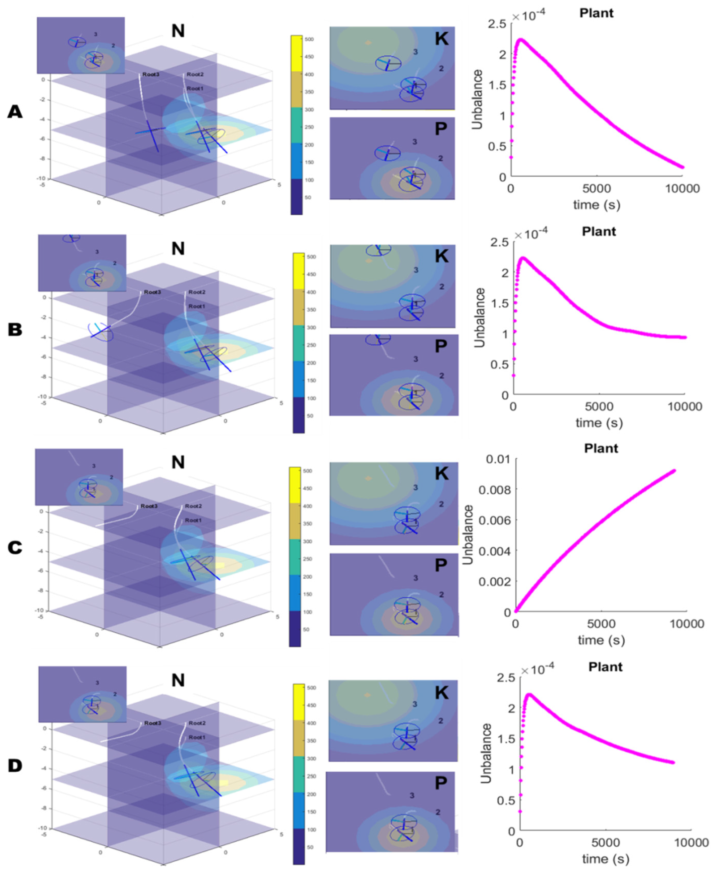
By comparing the control alternative A (Figure 7A) with the others (B, C and D), a different arrangement of the roots in the environment can be observed, suggesting that the use of dynamic priorities for each stimulus can greatly affect plant root architecture. The different arrangement of the roots induces a subsequent different perception and different uptake of nutrients. The curves of the nutrient imbalance highlight the trend of alternative C (Figure 7C) to completely diverge from zero. This thus suggests that the uptake–kinetics mechanism is fundamental for solving the plant wellness problem and the chemotropic response without the adjustment of nutrient priorities (similarly to the stimulus-oriented control previously developed) combined with other tropic responses are insufficient to ensure plant survival. In addition, the conversion function between and priorities is fundamental for establishing root architecture and a consequent faster or slower adjustment of nutrient balancing. In fact, the results of alternative B (Figure 7B), where a linear function was used instead of the quadratic function as in alternative A, show a different organization of the roots followed by a slower adjustment of the imbalance (on average, it reached ~4.9×10⁻⁵ at the end of the simulation, ~1.8 times higher than alternative A) (Table 3). In alternative D (Figure 7D), although the priorities are fixed (as in alternative B), there is an initial decrease in the imbalance. This is due to the variation in Michaelis–Menten parameters, which leads to a dynamic adjustment of the instantaneous uptake of nutrients. However, since this variation is not reflected in stimuli priorities, the root architecture is affected, inducing a deviation in the nutrient balance from the optimal condition.
Alternative A provides the best performance in terms of nutrient imbalance and was selected as the control for the robotic platform. The supplementary video (Supplementary Video S1) shows how each agent independently moves according to their internal state and local perception, and the immediate response of the uptake–kinetics mechanism that, as soon as the missing nutrient (P) is inserted in the environment, leads to a decreasing of the imbalance of nutrients in the whole plant.
4. Discussion and Conclusions
In this paper, plant roots are proposed as a source of inspiration for the design and architecture of robotic control. The behavior analysis from the literature led to the extraction of eight fundamental principles, which helped in the creation of a feedback control for a plant-inspired robotic platform (Plantoid).
The proposed control, inspired by the uptake–kinetics of plant roots and by the internal communication system of plants, was implemented in simulation and on the Plantoid, showing the effective directionality of root growth towards attractive stimuli and a natural adjustment of the internal nutrient balance. The control runs independently on each individual root agent and is able to dynamically adjust nutrient priorities for that agent alone on the basis of local memory and to direct its growth on the basis only of local and instantaneous perception.
Looking at the global architecture and internal state, roots are shown to organize themselves, leading to a collaborative behavior among the agents aimed at improving the equilibrium of nutrients and indeed plant wellness, thus autonomously satisfying Property 1, without the need of a centralized unit for the control of nutrient status and of tasks’ distribution on the agents. The swarming behavior is an emergent result of the auto-regulation adopted by the uptake–kinetics control and the redistribution of nutrients among the agents. We have shown, in fact, that the internal imbalance never seems to converge to optimality with a stimulus-oriented control (alternative C, lacking an uptake mechanism and priority adjustment) compared to the proposed uptake–kinetics feedback control (imbalance with alternative A 2.66×10⁻⁵ 546×10−5 imbalance with alternative C after ~3 h of simulated growth).
Even though, there is not confirmation from biology on how uptake and stimuli priorities are related, here, we have proposed the use of a quadratic function to map uptake–kinetics parameters into nutrients’ priorities, and by comparing this choice with the alternative that uses a linear function, we demonstrate that a priority function has an important role in defining root architecture and plant wellness. We show that the priority adjustment, independently actuated by each root, is a powerful instrument for the development of collaboration, without the need for a centralized unit to delegate task allocation.
The developed control can be used in artificial root-like robots, which can move for instance in rescue scenarios for survival detection, in unstructured environments for mapping, or in space exploration. Wellness can be defined according to the application, for instance by adjusting ratios among several and different stimuli, not necessarily chemical.
The work proposed here can be considered as a first milestone in plant-root inspired control, which can also contribute to understanding plant-root behavior. In fact, the implementation of hypothesis made on a biological model using a biomimetic platform, such as Plantoid, can help in hypothesis validation. For instance, the specific control can be incrementally adapted to include additional features of plant-root behavior in order to understand their role, e.g., the influence of temperature in Michaelis–Menten parameters and the subsequent influence on root distribution in soil. It would also be interesting to evaluate the energy costs of the biological model and use it as a nutrient consumption component on the control, observing how the behavior is affected. A subsequent evaluation would be how growth velocity is affected as well as an evaluation of the behavior when not all the absorbed nutrients are immediately sent to the shoot.
In terms of exploring the environment, it would be interesting to mimic lateral root growth not only from an engineering point of view for the development of new technological mechanisms but also analyzing how and where plants allocate new resources, i.e., roots, can lead to new ideas for collaborative exploration control strategies as well as for solving optimization problems.
Supplementary Materials
The following are available online at www.mdpi.com/2076-3417/8/1/47/s1, Video S1: Swarming Behavior Emerging from the Uptake–Kinetics Feedback Control in a Plant-Root-Inspired Robot.
Acknowledgments
The study was funded by Istituto Italiano di Tecnologia. The funding covers the costs of open access publishing.
Author Contributions
Emanuela Del Dottore performed the literature analysis, conceived the control, implemented and performed simulations and experiments, and wrote the paper; Ali Sadeghi designed and realized the robotic platform; Alessio Mondini designed and realized the electronics; Emanuela Del Dottore and Alessio Mondini discussed the control, experiments and results; Barbara Mazzolai oversaw, defined and advised on the research; and all the authors revised the paper.
Conflicts of Interest
The authors declare no conflict of interest.
References
- Bakule, L. Decentralized control: An overview. Annu. Rev. Control 2008, 32, 87–98. [Google Scholar] [CrossRef]
- Bonabeau, E.; Theraulaz, G.; Deneubourg, J.L.; Aron, S.; Camazine, S. Self-organization in social insects. Trends Ecol. Evol. 1997, 12, 188–193. [Google Scholar] [CrossRef]
- Beckers, R.; Goss, S.; Deneubourg, J.L.; Pasteels, J.M. Colony size, communication, and ant foraging strategy. Psyche 1989, 96, 239–256. [Google Scholar] [CrossRef]
- Seeley, T.D.; Camazine, S.; Sneyd, J. Collective decision-making in honey bees: How colonies choose among nectar sources. Behav. Ecol. Sociobiol. 1991, 28, 277–290. [Google Scholar] [CrossRef]
- Passino, K.M. Biomimicry of bacterial foraging for distributed optimization and control. IEEE Control Syst. 2002, 22, 52–67. [Google Scholar] [CrossRef]
- Wedde, H.F.; Farooq, M.; Zhang, Y. BeeHive: An efficient fault-tolerant routing algorithm inspired by honey bee behavior. In Proceedings of the International Workshop on Ant Colony Optimization and Swarm Intelligence, Brussels, Belgium, 5–8 September 2004; Springer: Berlin/Heidelberg, Germany, 2004; pp. 83–94. [Google Scholar] [CrossRef]
- Babu, L.D.D.; Krishna, P.V. Honey bee behavior inspired load balancing of tasks in cloud computing environments. Appl. Soft Comput. 2013, 13, 2292–2303. [Google Scholar] [CrossRef]
- Dorigo, M.; Birattari, M.; Stutzle, T. Ant colony optimization. IEEE Comput. Intell. Mag. 2006, 1, 28–39. [Google Scholar] [CrossRef]
- Kennedy, J. Particle swarm optimization. In Encyclopedia of Machine Learning; Springer: New York, NY, USA, 2011; pp. 760–766. [Google Scholar] [CrossRef]
- Brambilla, M.; Ferrante, E.; Birattari, M.; Dorigo, M. Swarm robotics: A review from the swarm engineering perspective. Swarm Intell. 2013, 7, 1–41. [Google Scholar] [CrossRef]
- Monshausen, G.B.; Gilroy, S. Feeling green: Mechanosensing in plants. Trends Cell Biol. 2009, 19, 228–235. [Google Scholar] [CrossRef] [PubMed]
- Gilroy, S.; Masson, P.H. Plant Tropisms; Blackwell Publishing: Ames, IA, USA, 2008; ISBN 9780813823232. [Google Scholar]
- Baier, M.; Hemmann, G.; Holman, R.; Corke, F.; Card, R.; Smith, C.; Rook, F.; Bevan, M.W. Characterization of mutants in Arabidopsis showing increased sugar-specific gene expression, growth, and developmental responses. Plant Physiol. 2004, 134, 81–91. [Google Scholar] [CrossRef] [PubMed]
- Rolland, F.; Baena Gonzalez, E.; Sheen, J. Sugar sensing and signaling in plants: Conserved and novel mechanisms. Annu. Rev. Plant Biol. 2006, 57, 675–709. [Google Scholar] [CrossRef] [PubMed]
- Tuteja, N.; Sopory, S.K. Chemical signaling under abiotic stress environment in plants. Plant Signal. Behav. 2008, 3, 525–536. [Google Scholar] [CrossRef] [PubMed]
- Alam, S.M. Nutrient uptake by plants under stress conditions. In Handbook of Plant and Crop Stress, 2nd ed.; Pessarakli, M., Ed.; Marcel Dekker, Inc. Publisher: New York, NY, USA, 1999; pp. 285–313. ISBN 9780824719487. [Google Scholar]
- Mazzolai, B.; Mondini, A.; Corradi, P.; Laschi, C.; Mattoli, V.; Sinibaldi, E.; Dario, P. A miniaturized mechatronic system inspired by plant roots for soil exploration. IEEE/ASME Trans. Mechatron. 2011, 16, 201–212. [Google Scholar] [CrossRef]
- Kim, S.W.; Koh, J.S.; Lee, J.G.; Ryu, J.; Cho, M.; Cho, K.J. Flytrap-inspired robot using structurally integrated actuation based on bistability and a developable surface. Bioinspir. Biomim. 2014, 9. [Google Scholar] [CrossRef] [PubMed]
- Li, S.; Wang, K.W. Fluidic origami with embedded pressure dependent multi-stability: A plant inspired innovation. J. R. Soc. Interface 2015, 12. [Google Scholar] [CrossRef] [PubMed]
- Akyol, S.; Alatas, B. Plant intelligence based metaheuristic optimization algorithms. Artif. Intell. Rev. 2016, 47, 417–462. [Google Scholar] [CrossRef]
- Yang, X.S. Flower pollination algorithm for global optimization. In Proceedings of the International Conference on Unconventional Computing and Natural Computation (UCNC 2012), Orléans, France, 3–7 September 2012; pp. 240–249. [Google Scholar] [CrossRef]
- Mehrabian, A.R.; Caro, L. A novel numerical optimization algorithm inspired from weed colonization. Ecol. Inform. 2006, 1, 355–366. [Google Scholar] [CrossRef]
- Salhi, A.; Eric, S.F. Nature-inspired optimisation approaches and the new plant propagation algorithm. In Proceedings of the International Conference on Numerical Analysis and Optimization (ICeMATH 2011), Yogyakarta, Indonesia, 6–8 June 2011. [Google Scholar] [CrossRef]
- Qi, X.; Yunlong, Z.; Hanning, C.; Dingyi, Z.; Ben, N. An idea based on plant root growth for numerical optimization. In Proceedings of the International Conference on Intelligent Computing, Nanning, China, 28–31 July 2013; Springer: Berlin/Heidelberg, Germany, 2013; pp. 571–578. [Google Scholar] [CrossRef]
- Zhang, H.; Yunlong, Z.; Hanning, C. Root growth model: A novel approach to numerical function optimization and simulation of plant root system. Soft Comput. 2014, 18, 521–537. [Google Scholar] [CrossRef]
- Sadeghi, A.; Mondini, A.; Del Dottore, E.; Mattoli, V.; Beccai, L.; Taccola, S.; Lucarotti, C.; Totaro, M.; Mazzolai, B. A plant-inspired robot with soft differential bending capabilities. Bioinspir. Biomim. 2016, 12. [Google Scholar] [CrossRef] [PubMed]
- Gruber, B.D.; Giehl, R.F.; Friedel, S.; von Wirén, N. Plasticity of the Arabidopsis root system under nutrient deficiencies. New Phytol. 2013, 163, 161–179. [Google Scholar] [CrossRef] [PubMed]
- Hodge, A. The plastic plant: Root responses to heterogeneous supplies of nutrients. New Phytol. 2004, 162, 9–24. [Google Scholar] [CrossRef]
- Macy, P. The quantitative mineral nutrient requirements of plants. Plant Physiol. 1936, 11, 749–764. [Google Scholar] [CrossRef] [PubMed]
- Van der Ploeg, R.R.; Kirkham, M.B. On the origin of the theory of mineral nutrition of plants and the law of the minimum. Soil Sci. Soc. Am. J. 1999, 63, 1055–1062. [Google Scholar] [CrossRef]
- Marschner, H. Mineral Nutrition of Higher Plants, 2nd ed.; Academic Press: London, UK, 1995; ISBN 9780124735439. [Google Scholar]
- Sumner, M.E. Application of Beaufils’ diagnostic indices to maize data published in the literature irrespective of age and conditions. Plant Soil 1977, 46, 359–369. [Google Scholar] [CrossRef]
- Epstein, E. Mineral Nutrition of Plants: Principles and Perspectives; Wiley: London, UK, 1972; ISBN 0-471-24340-X. [Google Scholar]
- Jungk, A.; Asher, C.J.; Edwards, D.G.; Meyer, D. Influence of phosphate status on phosphate uptake kinetics of maize (Zea mays) and soybean (Glycine max). Plant Soil 1990, 124, 135–142. [Google Scholar] [CrossRef]
- Siddiqi, M.Y.; Glass, A.D.; Ruth, T.J.; Rufty, T.W. Studies of the uptake of nitrate in barley I. Kinetics of 13NO3− influx. Plant Physiol. 1990, 93, 1426–1432. [Google Scholar] [CrossRef] [PubMed]
- Fortin, M.C.; Poff, K.L. Characterization of thermotropism in primary roots of maize: Dependence on temperature and temperature gradient, and interaction with gravitropism. Planta 1991, 184, 410–414. [Google Scholar] [CrossRef] [PubMed]
- Eapen, D.; Barroso, M.L.; Ponce, G.; Campos, M.E.; Cassab, G.I. Hydrotropism: Root growth responses to water. Trends Plant Sci. 2005, 10, 44–50. [Google Scholar] [CrossRef] [PubMed]
- Rhodes, A.L. Chemotropism of roots. Bot. Gaz. 1910, 50, 71. [Google Scholar] [CrossRef]
- Sun, F.; Zhang, W.; Hu, H.; Li, B.; Wang, Y.; Zhao, Y.; Li, K.; Liu, M.; Li, X. Salt modulates gravity signaling pathway to regulate growth direction of primary roots in Arabidopsis. Plant Physiol. 2008, 146, 178–188. [Google Scholar] [CrossRef] [PubMed]
- Hart, J.W. Plant Tropisms: And Other Growth Movements; Chapman & Hall: London, UK, 1990; ISBN 978-0-412-53080-7. [Google Scholar]
- Massa, G.D.; Gilroy, S. Touch modulates gravity sensing to regulate the growth of primary roots of Arabidopsis thaliana. Plant J. 2003, 33, 435–445. [Google Scholar] [CrossRef] [PubMed]
- Takahashi, N.; Yamazaki, Y.; Kobayashi, A.; Higashitani, A.; Takahashi, H. Hydrotropism interacts with gravitropism by degrading amyloplasts in seedling roots of Arabidopsis and radish. Plant Physiol. 2003, 132, 805–810. [Google Scholar] [CrossRef] [PubMed]
- Marty, F. Plant vacuoles. Plant J. 1999, 11, 587–599. [Google Scholar] [CrossRef]
- Lee, R.B.; Ratcliffe, R.G. Subcellular distribution of inorganic phosphate, and levels of nucleoside triphosphate, in mature maize roots at low external phosphate concentrations: Measurements with 31P-NMR. J. Exp. Bot. 1993, 44, 587–598. [Google Scholar] [CrossRef]
- Schenk, M.K.; Barber, S.A. Potassium and phosphorus uptake by corn genotypes grown in the field as influenced by root characteristics. Plant Soil 1980, 54, 65–76. [Google Scholar] [CrossRef]
- Mullen, J.L.; Wolverton, C.; Ishikawa, H.; Evans, M.L. Kinetics of constant gravitropic stimulus responses in Arabidopsis roots using a feedback system. Plant Physiol. 2000, 123, 665–670. [Google Scholar] [CrossRef] [PubMed]
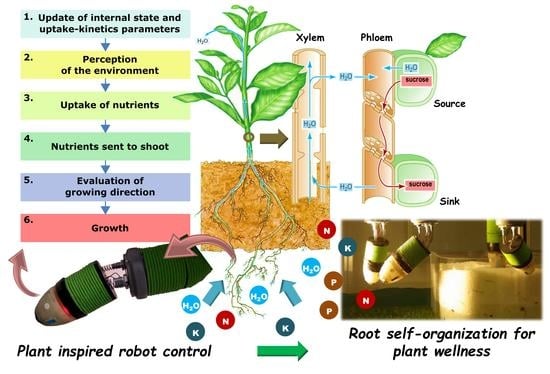
Figure 1.
The plant system. On the left, the biological model showing communication channels: the red arrow represents the monodirectional communication from root to shoot (xylem), while the blue arrow is the bidirectional communication along the whole system; on the root module, a schematic of ions uptake is presented with case (I) of internalization, case (II) of immediate sending to the shoot and case (III) storage in vacuole. On the right, there is the analogy with the plant inspired robot (Plantoid).

Figure 2.
An example of the virtual environment. Nutrients gradients are visualized over three separated spaces, one for each nutrient (N: nitrate, K: potassium, P: phosphorus) where the centers are, respectively, CN = (3, 2, −4), CK = (−3, −2, −1), CP = (3, 1, −5). Roots move in the environment where these three gradients coexist.

Figure 3.
Schematic of the uptake–kinetic feedback control. On the left, a detailed control diagram, and on the right, the workflow of the control showing the with sequential blocks of internal macro operations. Each root sends the quantity of each nutrient acquired from the environment to the shoot agent that redistributes values among all root agents. Internally, each root, after updating its memory, updates Michaelis–Menten parameters and nutrients’ priorities. On the second step, each root senses the environment and with the concentration perceived for each nutrient and its corresponding Michaelis–Menten parameters actuates the uptake and sends it to the shoot; with the same perception, each root performs also the evaluation of the next direction of growth that is obtained as combination between gravitropism and chemotropism.
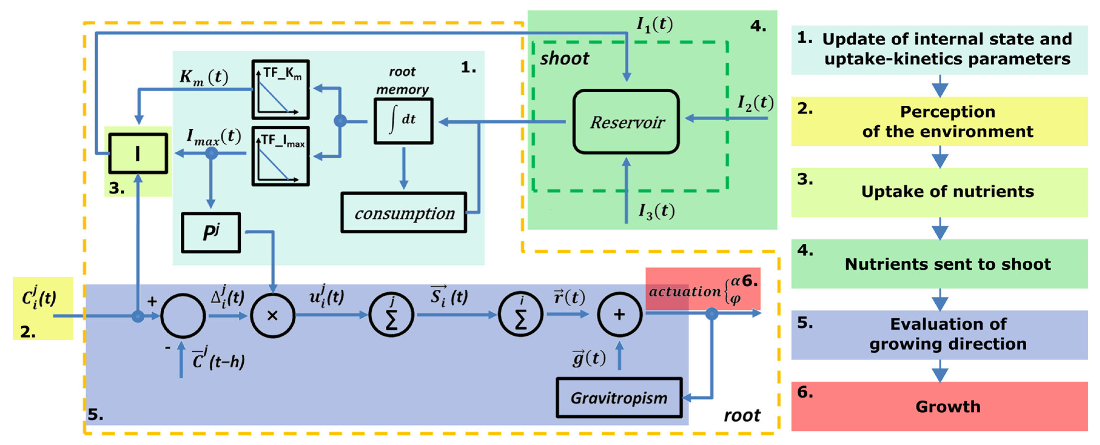
Figure 4.
Evolution of nutrients perception. An example of nutrients perception evolution for each root (three roots where placed in the environment) while growing. Case of nutrients with centers CN = (3, 2, −4), CK = (−3, −2, −1), CP = (3, 1, −5).
Figure 4.
Evolution of nutrients perception. An example of nutrients perception evolution for each root (three roots where placed in the environment) while growing. Case of nutrients with centers CN = (3, 2, −4), CK = (−3, −2, −1), CP = (3, 1, −5).

Figure 5.
Evolution of memory, nutrient priority and uptake. An example of evolution of internal memory, parameter and priority for Root 1. Case of nutrients with centers CN = (3, 2, −4), CK = (−3, −2, −1), CP = (3, 1, −5). The three roots with alternative A result with the same internal memory, and, consequently, they also have the same and priorities evolution. In the graphs, we can observe a face f1 where the internal availability of both N and K increases inducing a consequent decreasing of both and priority. When the internal availability starts to decrease, there is a consequent increasing of and priority (face f2).
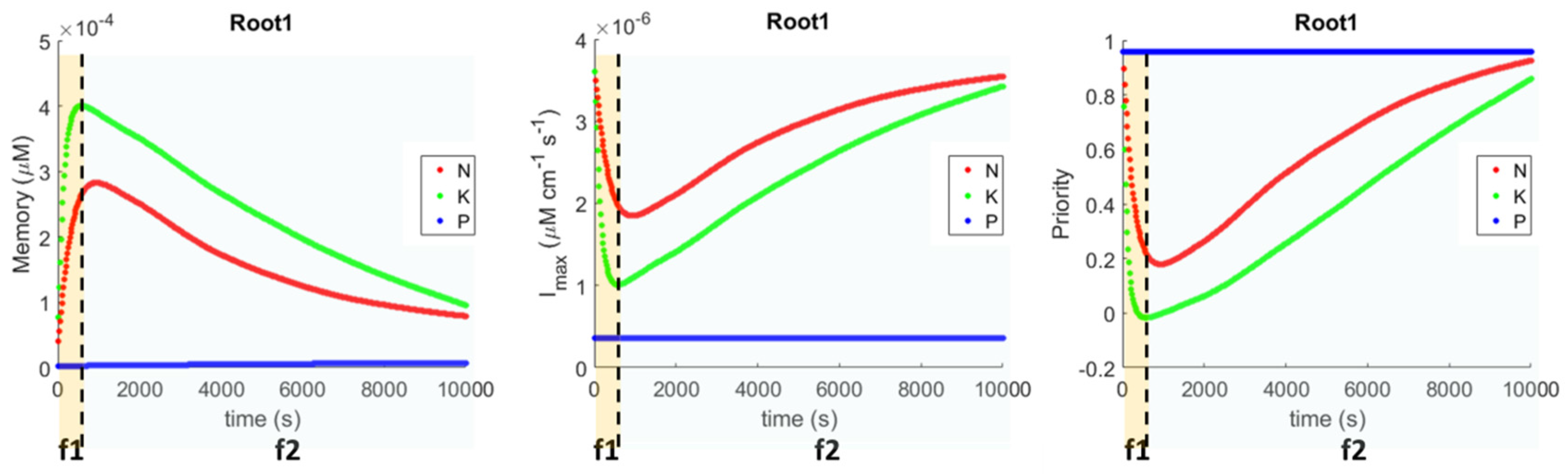
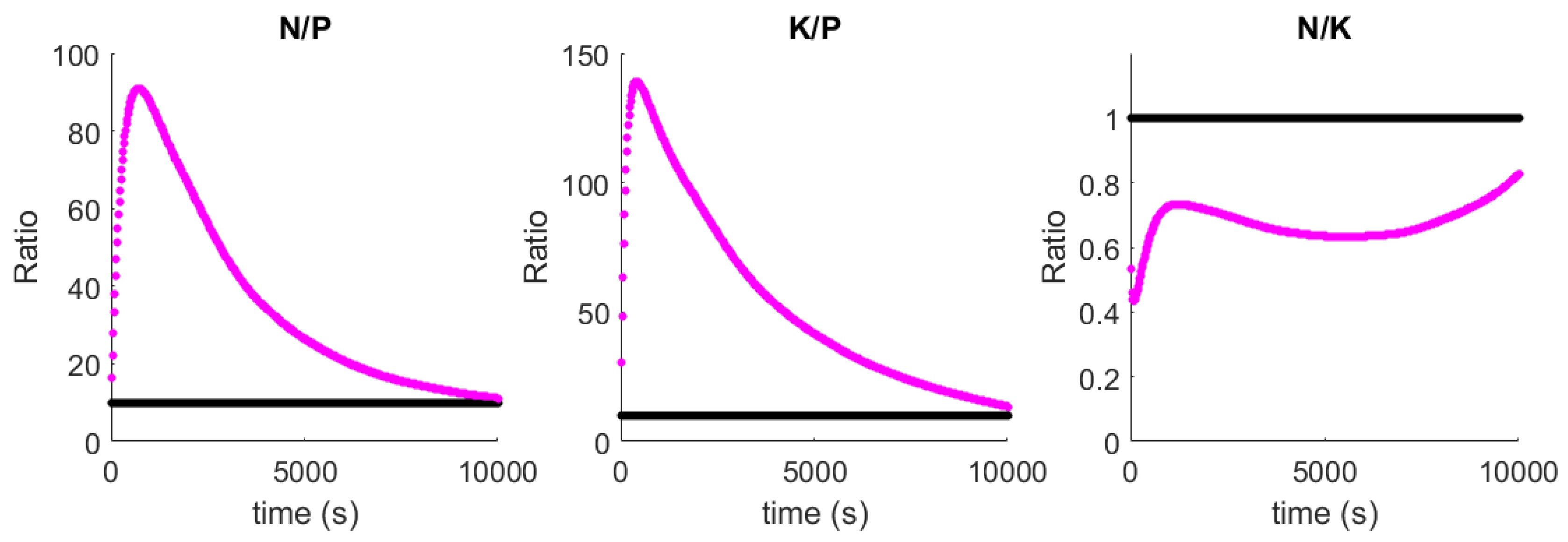
Figure 6.
Evolution of nutrients’ ratios. The evolution of nutrients ratios (in magenta color) in the entire plant while growing with alternative A in the case of nutrients with centers CN = (3, 2, −4), CK = (−3, −2, −1), CP = (3, 1, −5). The solid black lines represent the optimal nutrient ratios (N:P and K:P equal to 10 from [37]).

Figure 7.
Results of simulations. An example of simulation results after 10,000 s of growth. Roots started from positions: Root1 (0, 2, 0), Root2 (2, 0, −2) and Root3 (0, 0, 0). In the simulated environments, only the skeleton of the roots is visible, with the white lines depicting the region of maturity, blue lines the tip of the root and the circles depict the circumference of the root. The three roots are presented for alternative A: with the uptake–kinetic feedback control as presented in Section 2.5; alternative B: with the uptake kinetic feedback control where priorities function is a linear function; alternative C: where the control does not implement the uptake kinetic mechanism and priority adjustment; and alternative D: where the control implements the uptake kinetic mechanism but not priority adjustment. Each row in the figure presents from left to right: the root architecture at the end of simulation in the environment with nitrate, in the middle, the top view of the roots in the environments with potassium and phosphorus, and, on the right, the curves of nutrients imbalance.

Table 1.
Transformation functions. Coefficients of the linear functions used to obtain the parameters and of the uptake rate, given the internal concentration of each nutrient. The last column reports the points used for polynomial fitting. Considering that Michaelis–Menten parameters have been found to preserve the same ratios of nutrient requirement (N:P and K:P equal to 10 from [45]), points for fitting and , for nutrient N and K, were estimated from the values known for nutrient P at different concentration as found in the literature [34].
| p1 | p2 | Points Used for Fitting | ||
|---|---|---|---|---|
| Transformation function for (TF_Imax) y = p1×x + p2 | N | −6.992 × 10⁻³ | 3.672 × 10⁻⁶ | (0, 3.672 × 10⁻⁶), (5 × 10⁻⁴, 1.76 × 10⁻⁷) |
| K | −6.992 × 10⁻³ | 3.672 × 10⁻⁶ | (0, 3.672 × 10⁻⁶), (5 × 10⁻⁴, 1.76 × 10⁻⁷) | |
| P | −6.992 × 10⁻³ | 2.125 × 10⁻⁷ | (0, 3.672 × 10⁻⁷), (5 × 10⁻⁴, 1.76 × 10⁻⁸) | |
| Transformation function for (TF_Kmax) y = p1×x + p2 | N | −8.4 × 10⁻⁴ | 61 | (0, 61), (2 × 10⁻⁴, 19) |
| K | −8.4 × 10⁻⁴ | 61 | (0, 61), (2 × 10⁻⁴, 19) | |
| P | −8.4 × 10⁻⁴ | 6.1 | (0, 6.1), (2 × 10⁻⁵, 1.9) |
Table 2.
Parameters initialization. Initialization of the constants and storeCapacity used in the root agent control. Values of were fixed considering ratios N:P and K:P equal to 10 as found in the literature [34,45]. P was selected as the referential nutrient () and used for conversions and normalizations since it is the nutrient that has the lowest absolute value of the three nutrients required by plants.
| N | K | P | |
|---|---|---|---|
| 36.72 × 10⁻⁷ μM cm−1 s−1 | 36.72 × 10⁻⁷ μM cm−1 s−1 | 36.72 × 10⁻⁸ μM cm−1 s−1 | |
| storeCapacity | 0.002 μM | 0.002 μM | 0.0002 μM |
Table 3.
Nutrient imbalance. Nutrient imbalance obtained at the end of simulation (~3 h of simulated growth), for each of the control alternatives. Resulting imbalance is obtained as the averaged imbalance over three different runs, placing the centers of nutrients at different random locations: RUN 1 CN = (3, 2, −4), CK = (−3, −2, −1), CP = (3, 1, −5); RUN 2 CN = (−3, 3, −4), CK = (−3, −2, −3), CP = (1, 1, −5); RUN 3 CN = (1, 2, −2), CK = (4, 1, −1), CP = (2, 1, −2).
| A | B | C | D |
|---|---|---|---|
| 2.66×10⁻⁵ | 4.93×10⁻⁵ | 546×10−5 | 5.69×10⁻⁵ |
© 2018 by the authors. Licensee MDPI, Basel, Switzerland. This article is an open access article distributed under the terms and conditions of the Creative Commons Attribution (CC BY) license (http://creativecommons.org/licenses/by/4.0/).
Share and Cite
MDPI and ACS Style
Del Dottore, E.; Mondini, A.; Sadeghi, A.; Mazzolai, B. Swarming Behavior Emerging from the Uptake–Kinetics Feedback Control in a Plant-Root-Inspired Robot. Appl. Sci. 2018, 8, 47. https://doi.org/10.3390/app8010047
AMA Style
Del Dottore E, Mondini A, Sadeghi A, Mazzolai B. Swarming Behavior Emerging from the Uptake–Kinetics Feedback Control in a Plant-Root-Inspired Robot. Applied Sciences. 2018; 8(1):47. https://doi.org/10.3390/app8010047
Chicago/Turabian StyleDel Dottore, Emanuela, Alessio Mondini, Ali Sadeghi, and Barbara Mazzolai. 2018. "Swarming Behavior Emerging from the Uptake–Kinetics Feedback Control in a Plant-Root-Inspired Robot" Applied Sciences 8, no. 1: 47. https://doi.org/10.3390/app8010047
Note that from the first issue of 2016, this journal uses article numbers instead of page numbers. See further details here.