Passive Sonar Target Detection Using Statistical Classifier and Adaptive Threshold

Department of Electrical and Computer Engineering, University of Birjand, Birjand 97175, Iran
*
Author to whom correspondence should be addressed.
Appl. Sci. 2018, 8(1), 61; https://doi.org/10.3390/app8010061
Submission received: 16 September 2017
/
Revised: 24 December 2017
/
Accepted: 27 December 2017
/
Published: 3 January 2018
Abstract
:This paper presents the results of an experimental investigation about target detecting with passive sonar in Persian Gulf. Detecting propagated sounds in the water is one of the basic challenges of the researchers in sonar field. This challenge will be complex in shallow water (like Persian Gulf) and noise less vessels. Generally, in passive sonar, the targets are detected by sonar equation (with constant threshold) that increases the detection error in shallow water. The purpose of this study is proposed a new method for detecting targets in passive sonars using adaptive threshold. In this method, target signal (sound) is processed in time and frequency domain. For classifying, Bayesian classification is used and posterior distribution is estimated by Maximum Likelihood Estimation algorithm. Finally, target was detected by combining the detection points in both domains using Least Mean Square (LMS) adaptive filter. Results of this paper has showed that the proposed method has improved true detection rate by about 24% when compared other the best detection method.
1. Introduction
Due to the severe attenuation of radio frequency and optical signals under the sea, the use of audio signals is often a great way to detect under water targets. Sonar (Sound Navigation and Ranging) is a technique that uses sound propagation to navigate, communicate with or detect objects on or under the surface of the water, such as other vessels. These systems record the sound waves using hydrophone and by processing these signals, we can detect, locate, and classify different targets. Sonar is divided into two families of active and passive that in the active type, by sending sound pulses (pings) and analyzing the echoes of them, we can identify the type, distance, and direction of the target. In the passive sonar, which is the topic of the project, underwater acoustic signals received by the hydrophone and after pre-processing, signal can be detected by analyzing the content of the target. The passive sonars use waves and their unwanted vibrations to identify vessels.
Sounds do not generate only from the vessels so the factors such as waves, vibrations from the bottom of sea, fishes, and so on cause confusion target detection. Therefore, for target detecting, we need an intelligent adaptive threshold level that at the different situations and environmental parameters to minimize error detection. Typically, the detection of sonar targets is performed using sonar equations. These equations have many variables, such as the source level, the transmission path loss, reflection lose, sound absorption, and so on that some of them are the functions of other variables.
In this method, the source level (SL) is a measure of the acoustic intensity of the signal measured one meter away from the source. This parameter assumes that the acoustic energy spreads omnidirectionally outwards away from the source. However, most acoustic sources are designed to focus the acoustic energy into a narrower beam in order to improve efficiency. This effect is accounted for in the sonar equations by the Directivity Index (DI) as a measure of focusing. The Detection Threshold (DT) is a parameter defined by the system. If the observed signal to noise ratio exceeds the detection threshold, then a target is assumed to be present. The intensity of an acoustic signal is reduced by range. This reduction in the acoustic signal with distance from the source is due to the combined effects of spreading and attenuation and is accounted by the transmission Loss Term (TL). The Target Strength (TS) is a measure of how good an acoustic reflector the target. The echo level will increase with target strength.
Figure 1 shows the relationship between the various components of the hydrophone sonar arrays and decisions about the presence/absence of target.
Target detection with passive sonar has found to be so interesting for many researchers during last ten years. Generally, target detection algorithms are applied in three domains: in time domain, in frequency domain and fusion time-frequency domain. Later, in time domain, Urick performed a combined experimental and numerical study to investigate Sonar Equation for calculate signal to noise ratio in [1]. Nielsen in [2] reported that DEMON (Detection Envelope Modulation on Noise) narrowband analysis that furnishes the propeller characteristic: number of shafts, shaft rotation frequency and blade rate of the target. Dawe reported in [3] that using Receiving Operating Characteristics (ROC) curve improves the target detection performance in Sonar Equation. Chin et al. performed Two-Pass Split-Windows (TPSW) algorithm and Neural Network to classify under water signal [4]. Abarahm performed non-Gaussian function for determines Detection Threshold (DT) in [5]. Wakayama et al. describes the forecasting of probability of target presence in a search area [6] (also referred to as the PT map) when considering both detection and non-detection conditions. Kil Woo et al. describes DEMON algorithm for detecting target in passive sonar [7]. The reported method in [8] focused on the performance of the normalized matched filter (NMF). The NMF is used when the noise covariance matrix is fast time-varying and is hard to estimate. The proposed method in [9] to handle the nonlinearity between target states and the raw bearing measurements, particle filter is employed to compute the joint multi target probability density (JMPD) recursively through a Bayesian framework. After detection, Target recognition (classification) and tracking are used.
In frequency domain, Martino performed LOFAR (Low Frequency Analysis and Recording) broadband analysis, estimates the noise vibration of the target machinery [10]. Borowski and et al. in [11] investigated analysis under water signal in frequency domain. Zhishan Zhao et al. proposed an improved matched filter in Additive white Gaussian noise (AWGN) combined with the adaptive line enhancer by analyzing the output spectrum and the spectral spectrum of the matched filter, which is the frequency-domain adaptive matched filter. Note that this method is proposed for active sonar [12]. In this paper [13], Mel frequency Cestrum Coefficients feature extraction using sound pressure and particle velocity signals are researched. Firstly, Mel-Frequency Cepstral Coefficients (MFCC) feature, first-order-differential MFCC feature, and second-order differential MFCC feature can be used as the effective feature of the underwater target identification from the feature extraction and recognition results. Secondly, by calculating the Fisher-ratio and correlated distance, it can be found that the contribution of each dimension feature is different, and those three features that are fused by using fdc criterion can improve the recognition probability of underwater target signal.
In fusion domain, Moura et al. in [14] performed independent component analysis for detection and classification of signals against background noise by using time and frequency domain. Sen Gupta et al. in [15] proposed new method for detecting a target in non-stationary clutter in active sonar using dynamic time-frequency localization. In [16,17], authors try to estimate behavior of target motion by using Target Motion analysis (TMA) and Bearing Only Tracking (BOT) algorithms. Note that TMA and BOT are used after detection. Thus, accurate detection is vital for TMA and BOT algorithms.
In this paper, a new method for detecting targets in passive sonars using adaptive threshold in fusion domain is proposed. In this method, target signal (sound) is processed in time and frequency domain. For classifying, Bayesian classification is used and posterior distribution is estimated by Maximum Likelihood algorithm. Finally, target was detected by combining the detection points in both domains using Least Mean Square (LMS) adaptive filter. The paper is organized as follows. In Section 2, we describe proposed novel algorithm for target detection with passive sonar in shallow water. In Section 3, we discuss a method of calculate detection point in time and frequency domain and fusion to determine adaptive threshold and advantages. In Section 4, we present the experimental results on vessel signals recorded in Persian Gulf (Figure 2). Finally, we conclude the proposed method in Section 5, and present an attempt a critical evaluation.
2. Target Detection in Passive Sonar
Target detection, is as the separation of a special signal that is “target” from the other signals. In other words, in the case of detection, all of the received signals are divided into target and non-target classes by classifier. In general, non-target signals are regarded as noise/clutter and a successful classifier is one that uses (the least) existing knowledge to extract the target signal from the noise.
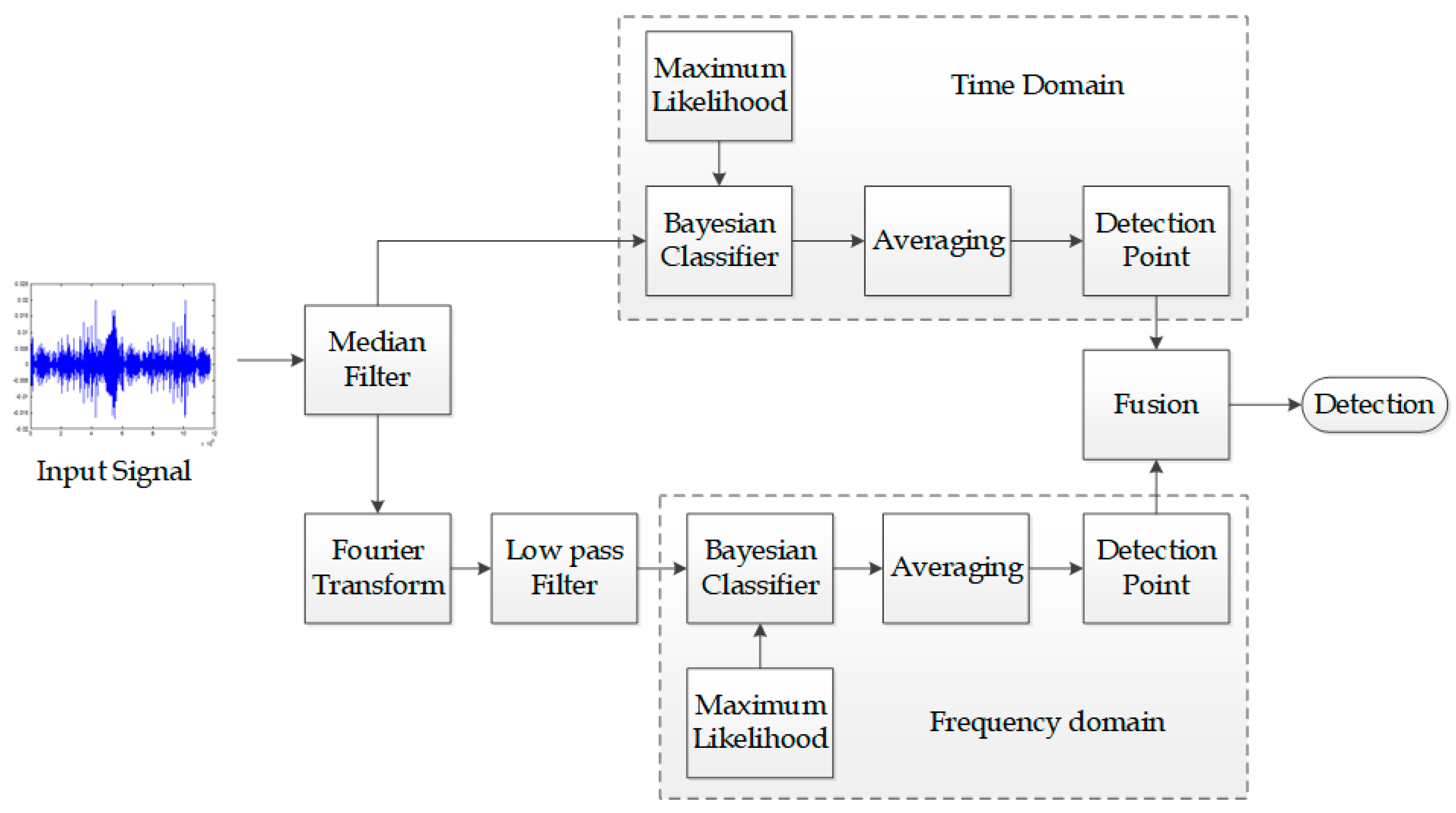
Over the years’, researchers have used several classifiers to extract target signal from noise, such as support vector machines (SVM), neural networks, and statistical classifier. In this article, according to the statistical of the environment of the sea and the condition of targets (which are mostly fluctuating), Bayesian statistical classifier method has been used. In the proposed method, after pre-processing, the Bayesian filter is trained by the target signal and noise in time and frequency domain. For calculating the coefficients of posterior distribution, MLE (Maximum Likelihood Estimation) algorithm is used. Results of Bayesian classification in each domain are recorded as detection point and fusion is done by Winer adaptive filters. Finally, the appropriate adaptive threshold for detection is calculated. Briefly, the proposed method is shown in Figure 3. In following, ambient noise, radiation noise, and the details of the proposed method and the obtained results are presented.
2.1. Ambient Noise
The noise that is received by an Omni-directional hydrophone in the underwater heterogeneous environments is the ambient noise. Ambient noise level is measured by an Omni-directional hydrophone from the noise power ratio to the Omni-directional base plate hydrophone. Sources of underwater noise emissions in the environment have a bandwidth of 1 Hz to 100 KHz, which cover all frequency-existing. In order to examine the factors that are affecting ambient noise according to depth, the noise can be divided into two categories in deep-water and shallow water noise.
2.2. Radiated Noise
Ships, submarines, and torpedoes are among the sources of radiated noise. This type of noise includes machinery radiated noise, ship propeller noise, and hydrodynamic noise emission. Noise caused by turbulence, which is caused by floating propeller and water bubbles floating in the back of the vessel are broadband, and often gives cover to 10 kHz. However, the power of this noise is more under 3 kHz. Sonar noise is not white, but it is mixed with strong frequency components (above the noise level). These components are caused by the fact that, for example, in floating motor pistons, camshafts and blade-butterfly are moving out with a certain velocity relative to each other, and create slim but strong frequency components that depending on the engine speed, their power is different from each other.
3. Statistical Classifier and Adaptive Threshold
The base of this research is detecting incognito sounds from background sounds. Perhaps a sound of glass or an unknown object that drops on the ground dark and silence room be a good example to express the main idea of this article. In this study, each sound divided to environment sound (which is called ambient noise) and target sound. These sounds are compared by the recorded ambient noise (training signal) and their similarities will be determined numerically by detection points. In the following, how to calculate detection point is described.
As shown in Figure 3, to reduce the input noise, a median filter is applied. So, Bayesian classification algorithm has been used to classify signal from noise in both time and frequency domains. The result of classification is averaged at the time domain and then the detection points are calculated. In the frequency domain (like time domain), the signal passes through the low-pass filter, then after classify by Bayesian classification, detection point is calculated by averaging. Final detection point is obtained after fusion detection points in time and frequency domains by the adaptive Wiener filter.
3.1. Detection Point in Time Domain
In this study, Bayesian algorithm is used to classify input signal. The target and noise signal have pseudo-Gaussian distribution, so applying the Bayesian algorithm has shown good results for extracting the target signal. To classify the target signal, the statistical distribution of the target signal and noise are estimated using training data. In this algorithm, if θ represents label of target (s), noise (b), and x be a member of the input vector of the sound signal, the prior distribution the probability of noise and the target, Gaussian density function is the probability of the x value occurrence in the region of θ and the posterior distribution is defined by (1):
The Gaussian density function is calculated by (2):
where . The mixture parameters , i = 1, 2 can be initialized and updated using the MLE [18] algorithm. This algorithm is explained by (3):
where, is weights of normal distribution, and is mean and variance of distribution in kih iteration .Convergence condition is .
Finally, by estimate posterior distribution and based on (4) similar target signal () is separated from ambient noise ().
As mentioned, the classifier is performed in time and frequency domains. In the time domain, after classifier input signal (with lengths 10 thousand samples) into two classes of 0 (noise) and 1 (target), the resulting output has much continuity and discontinuity in some areas which due to the statistical similarity of target signal with noise. To solve the problem, the signal integrity characteristic of the target is used. In other words, the target signal has sectional continuity, which is also due to the continuous movement of the vessel propeller in the water. The marine diesel engines are turned on and off with bare-speed, and thus a sharp break does not occur in the propeller’s sound.
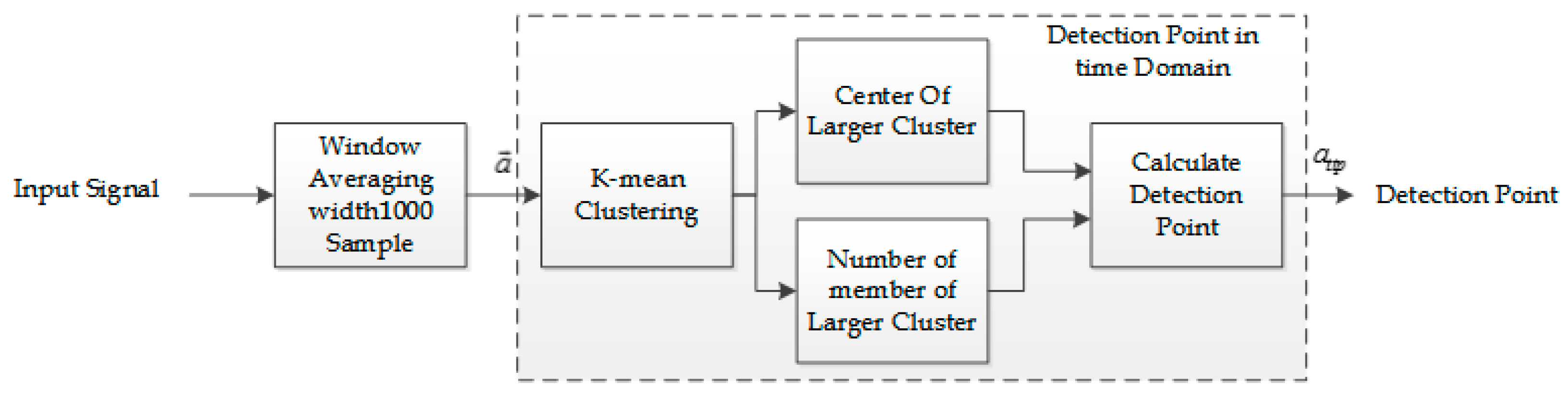
Thus, the result of classification is averaged by a windows with a width of w = 1000, which is selected experimentally and it is stored in a vector called mean vector . In (5), how calculation this vector is shown. In this equation, n is number of sample and x(.) is the input signal.
For calculation detection point, K-means (with K = 2) clustering algorithm is used. In this method, when considering K-means clustering algorithm, vector is divided to two clusters, target and non-target. In Bayesian classifier, target label is selected 1 and non-target is selected 0, so in this paper, center cluster that close to 1 is selected as detection point (blue circles in Figure 4a). According to a survey conducted, it is a necessary condition that the center of cluster is close to 1, but it is not sufficient. As shown in Figure 4b, it is possible noise signal has similarity in the behavior with target signal, thus in the noise signal (without present target) the greater center cluster is close to 1 is selected as detection point and detection point increased incorrectly.
In this study, to solve this issue (shown in Figure 4b), greater center of cluster and number of its members determine detection point. If the center of each cluster and number of its members is greater, then the signal is similar to target and detection point increase correctly. In (6) how calculate detention point in time domain is expressed.
where the detection point in time domain for per 1000 samples is , the greater center of cluster is , the number of its members is nMt, and the whole number of members is nt. Since the input signal is added with ambient noise (with same size and in K-means Algorithm K = 2, to correct the error clustering of signals without any noise, equation is multiplied by 2. In the other hands in ideal condition, nMt = 0.5nt. In summary, Figure 5 shows how to calculate detection point in time domain.
3.2. Detection Point in Frequency Domain
To increase true detection rate, we need more features that was extracted in time domain. Because of present high ambient noise in the shallow water, analysis input signal in other domain (like frequency or wavelet domain) obtained more information to detect low amplitude signal or silence target. On the other hand, many times features that extracted in time domain in not enough to detect silent target in shallow water correctly. Experimental result shown fusion detection points in time and frequency domain increase true detection rate effectively. So, in this section (according to Figure 3) input signal (10 thousand samples) after passing through a low pass filter and use Fourier transform will be separated into two clusters, which are labeled by 0 (noise) and 1 (target). The sound of propeller is in the lower band, so the low-pass filter is proposed.
Output of filter is averaged by a window with a width of w = 100 (which is selected experimentally) and it is stored in a vector called mean vector . Then, with using K-means Clustering algorithm like time domain, detection point in frequency domain is calculated by (7).
where the detection point for per 100 samples in frequency domain is , the larger cluster center is , the number of its members is , and the whole number of members is . Because of the number of cluster in K-mean algorithm is 2, to correct the error clustering of signals without any noise, the equation is multiplied by 2. In summary, Figure 6 shows how to calculate detection point in frequency domain.
3.3. Target Detection
As shown in Figure 3 for target detection, detection point is calculated in the time and frequency domains and the sum of these two values will determine the final detection point. If condition (8) satisfied, then the target is detected.
With respect to condition (8), the sum of two detection points directly, may increase the error detection. This fault usually is created due to climate changes, air, and water, the location of the sonar and etc. To reduce the error rate, detection point in both the time and frequency domain has been combined. Various methods for fusion are proposed. For example, Ciuonzo et al. in [19] proposed new decision fusion to provide a systematic taxonomy of the viable detectors. In this paper, to reduce the error rate, detection point in both time and frequency domain has been combined by adaptive weigh. The weights are calculated by Wiener filter. In other hand, because of changing environmental conditions (depth, heat, pressure…) in deferent points of sea the ambient noise signal is changed randomly. So for decrease effect of environmental conditions, winner filter is proposed. In this paper detection point (in both time and frequency domain) has been combined by adaptive weight that calculated by winner filter. This filter is updated by LMS algorithm.
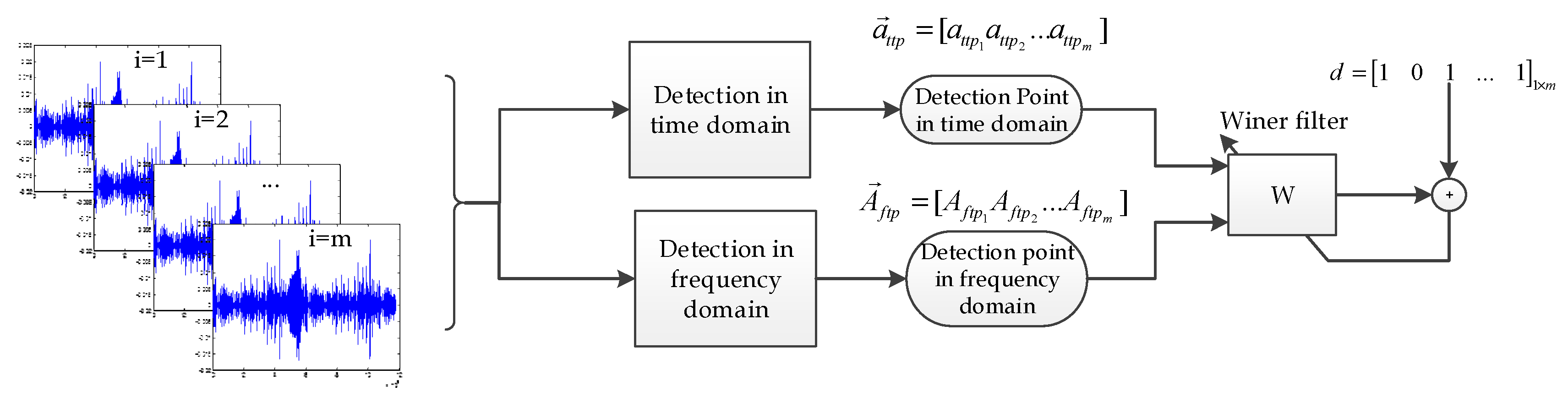
Figure 7 indicated calculation adaptive detection point by Winer filter.
In this study, the Wiener filter coefficients w and W (is shown in (9)) is calculated by LMS method.
where the detection point vector in m sequence of test input signals (which 10 thousands sample length in each sequence) in time domain, is the detection point of ith sequence in m sequences in time domain, is detection point in m sequence of test input signals in frequency domain, is the detection point for ith sequence in m sequences in frequency domain, w and W are the Wiener filter coefficients, and Detection Point (DP) is detection point after fusion. In this case, the condition (8) changes to condition (10).
In other words, to estimate the target signal, m sequence of input signal (test) is investigated and eventually checking detection points in m sequences, the presence or absence of the target is determined.
4. Experimental and Simulation Results
In this study, for simulating and analyzing the performance of the proposed method the database available on the Noar Institute (Copyright) is used. This database contains commercial vessels’ sound and Persian Gulf’s environmental noise. In this study, using actual environmental noises and the sound of the propeller detection is performed and the results are compared with conventional methods of detection sonar equations. The following steps are simulated and the proposed method is compared with conventional methods.
4.1. Simulation Steps
According to Figure 3, the results of the proposed method is expressed on a database that includes pre-processing, classifying, averaging, fusion, and finally detecting. In the first database is described, then the results are expressed.
4.2. Database
In the database of Noar Institute 25 unique voices of propellers of commercial vessels, such as oil tankers for 30 to 120 s and 15 ambient noises (sound of waves of the sea, rain...) for 10 to 30 s are present. As well as 25 real audio signals, which contain vessels and environmental noise, some of them are more than one vessel and move at different distances.
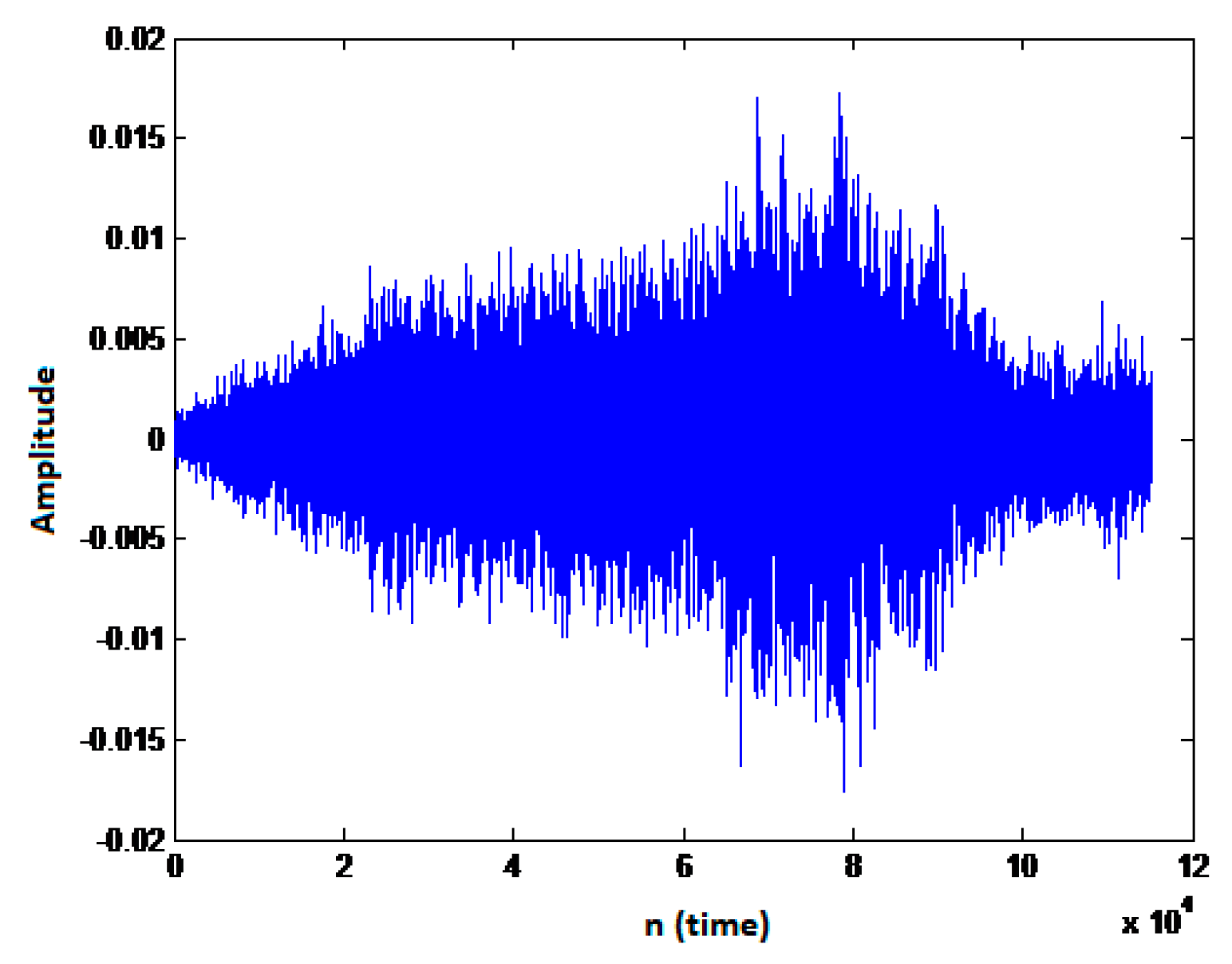
These sounds have been recorded by hydrophone at a depth of 10 m and environmental noise when there is no vessel in a specified distance exists is recorded. Environmental noises, including sound of sea waves, sound of sea floor, the sound of rain, and more. As mentioned the vessels are tankers, merchant ships and etc. In this study, the input (Background noise) to over 10 thousand sample sounds division and a sampling rate is 44 Kbps. It is worth noting the signal after the normalization is used. Figure 8 is an example of propeller sound. Figure 9 shows an example of ambient noise signal. In database, the target training signals, due to their proximity to the hydrophone have little noise. In his words, the target signals themselves are mixed with ambient noise which is the nature of underwater sound. Figure 10 shows an example of the mixed sounds (noise and the target). For example, in sample number 500 thousand a vessel in 3 km distance and in sample 1 million another vessels at a distance of 8 km exist.
To train the Bayesian algorithm and LMS, the signal of environmental noise and target with 10 thousand samples have been used. The training signals are made up of noise and the target signal (mixed with noise) that the first five-thousand samples are ambient noise and the second five-thousand samples are the mixed signals. In all cases, after train Bayesian classifier the white noise is added to the recorded ambient noise to increase challenge complexity.
4.3. The Simulation Results
The median filter is applied normalized input signal (Figure 9), and some low and high frequency noises are removed. The reason of using this filter is some high-frequency noise on the input signal.
After applying the median filter, the output signals are divided to a sequence of signal with 10 thousand sample length. Bayesian algorithm is applied on these signals in both Fourier and time domain.
In the time domain to train the Bayesian algorithm, two groups of the target signal and ambient noise signals are used. According to the input signal, mean and variances values of posterior function are calculated. In the frequency domain signal input is passed from low-pass filter and after calculating the Fourier coefficient as proposed in the time domain, main and variance values of the posterior function are calculated. After determining the values in time and frequency domains, detection points will be calculated by fusion. Following how calculation the detection point and simulation results is expressed.
4.4. Calculation of Detection Points in the Time Domain
After applying Bayesian algorithm in the time domain, the output will be labeled with 1 (target) and 0 (noise). An example of this classification is shown in Figure 11.
To reduce classification error of Bayesian algorithm, the labeled signals are averaged by window width w samples. The averaged values recorded at the center of the window provides mean vector. Figure 12 shows an example of this vector. To increase challenge complexity input signal is reconstructed by (11).
where is reconstructed input test signal, target is propeller or ship engine sound, and noise is ambient is mixed by white noise. For only noise input, target is null.
In this paper, the length of input test signal is 10 thousand sample (n = 10,000) and the width of the average window is selected five-thousand (w = 5000) sample, so the sample size of the vector has been reduced to 20. As shown in Figure 12, because of present target from five-thousand, detection point is increased after number 10.
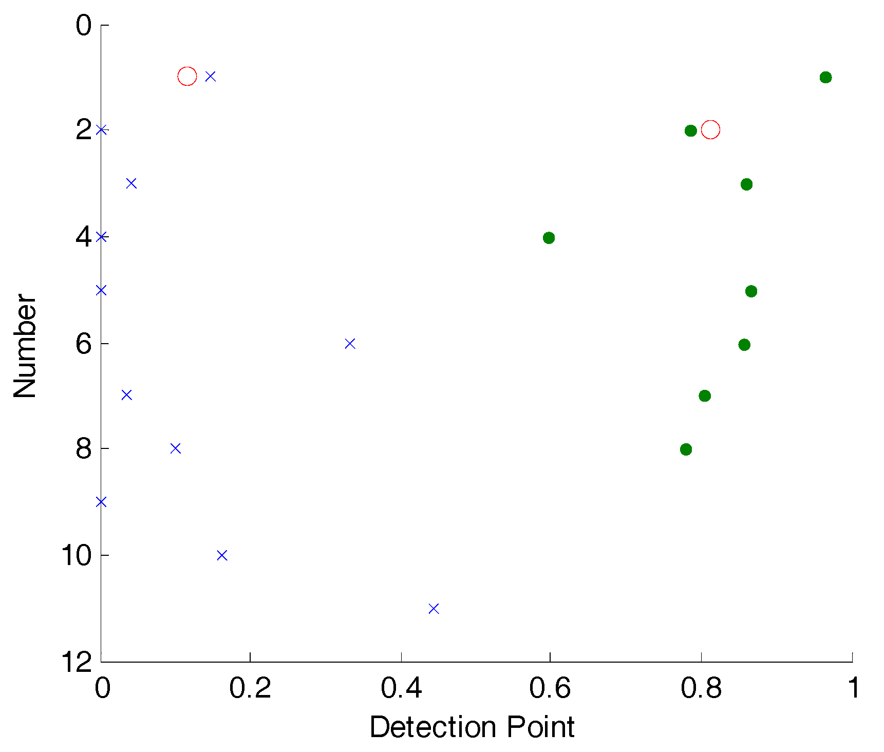
As shown in Figure 5, the clustering algorithm K-means has been used for average vector. The result is shown in Figure 13. In this figure, dots shown elements of the first cluster, crosses shown elements of the second cluster, and the hollow circles are the cluster center.
In Figure 13 the greater center of cluster (close to 1) is 0.8 and the number of its elements is 8 (from 20). According to the proposed algorithm, the detection point is calculated by the Equation (2), Table 1 shows detection point of 19 test signals in a specific sequence in the time domain.
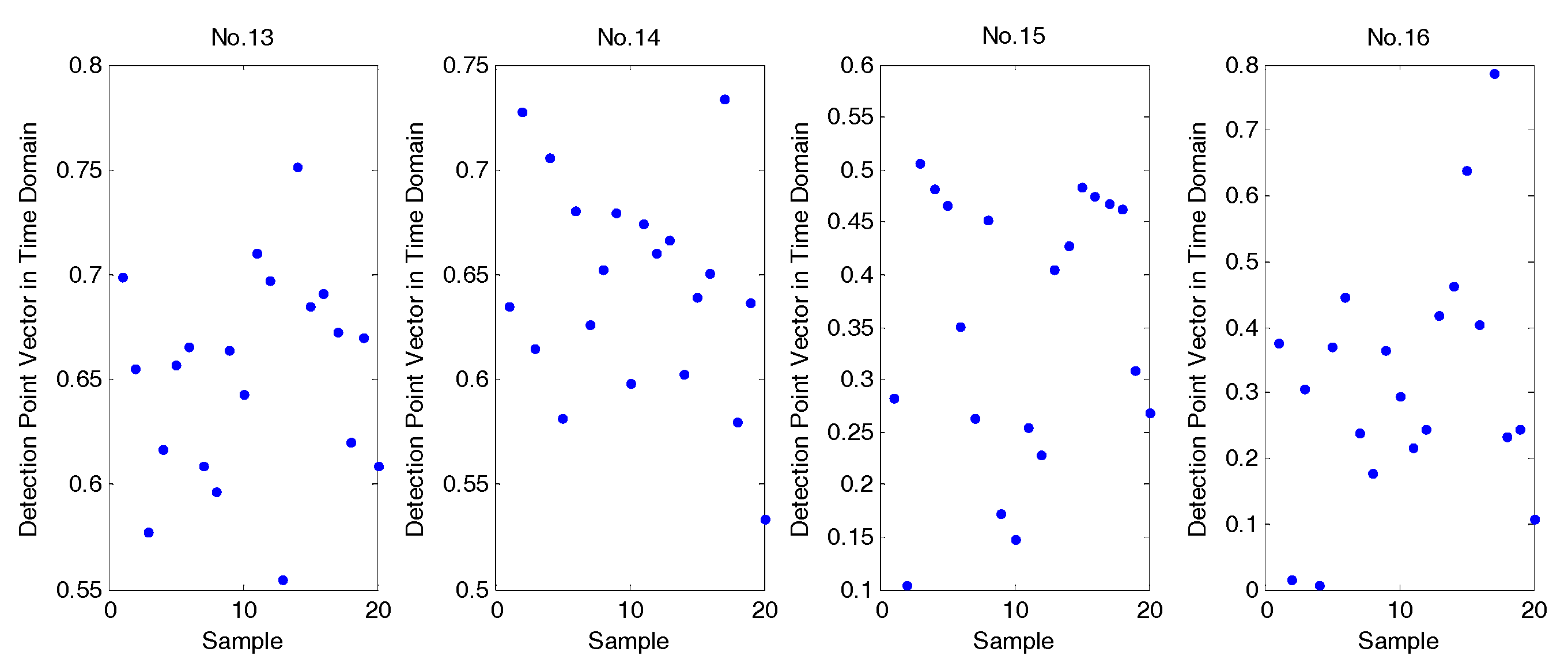
Figure 14 shows the vector for four test input signals (No. 13 to 16) in the time domain.
4.5. Calculation of Detection Points in the Frequency Domain
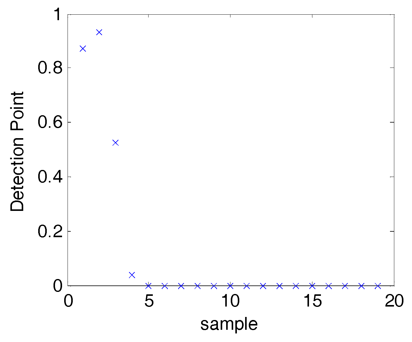
The calculation of detection points in the frequency domain is similar to the proposed method in time domain, but, as shown in Figure 6, the input signal is passed through a 2 kHz low-pass filter. Then Fourier coefficient is calculated with two-thousand samples. As explained, the width of averaging window is selected 100 (w = 100) so the length of the vector will be the average with 20 samples. As shown in Figure 15 because of present target in low frequency, first term coefficients is greater than other. After the calculation of vector, , as is shown in Figure 6 the detection points are calculated in frequency domain. Table 2 shows an example of the detection points for 19 test input signals.
.
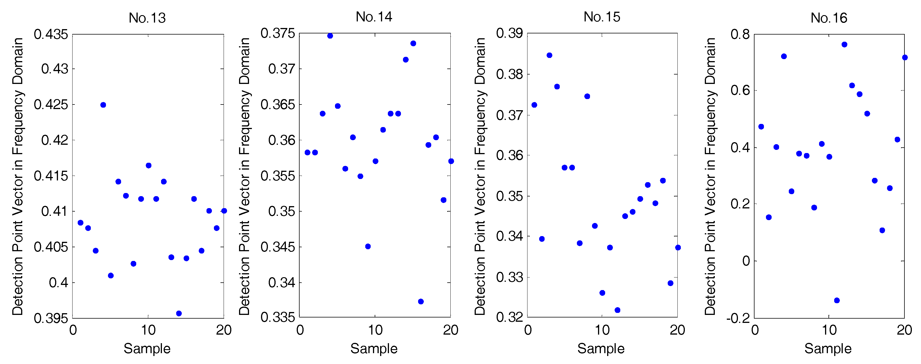
Figure 16 shows the vector for four test input signals (No. 13 to 16).
4.6. Fusion
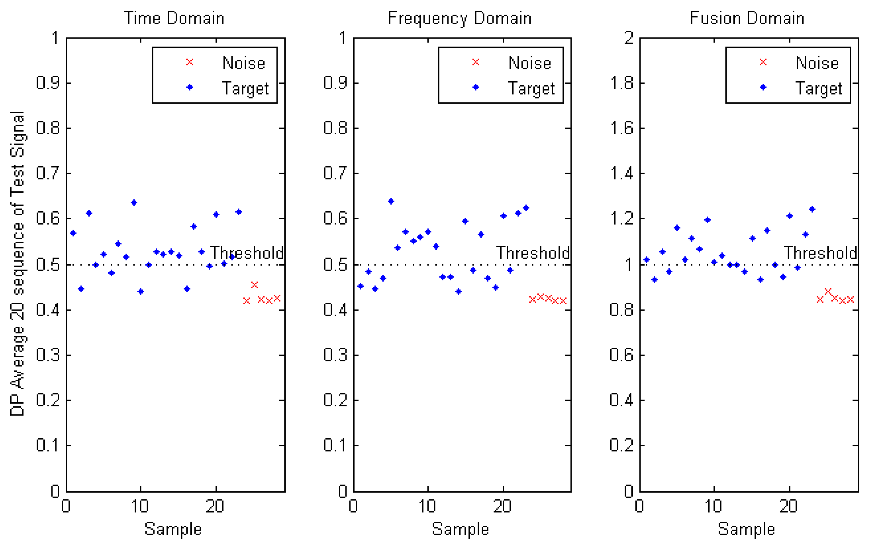
In this paper, two methods for fusion detection point in the time and frequency domains are expressed. In the first method, detection points in these two domains are directly combined. As stated before, in this method, the detection error is increased due to environmental conditions. Figure 17 shows the average of 20 sequences (m = 20) for 19 test signals (1 to 14 target signals and 15 to 19 are the ambient noise signals). As shown in Figure 17 (Fusion Domain), the distance between the DP of target and noise is very small and close to the threshold 1, and this caucuses to increase the detection error.
The second method, which is shown in
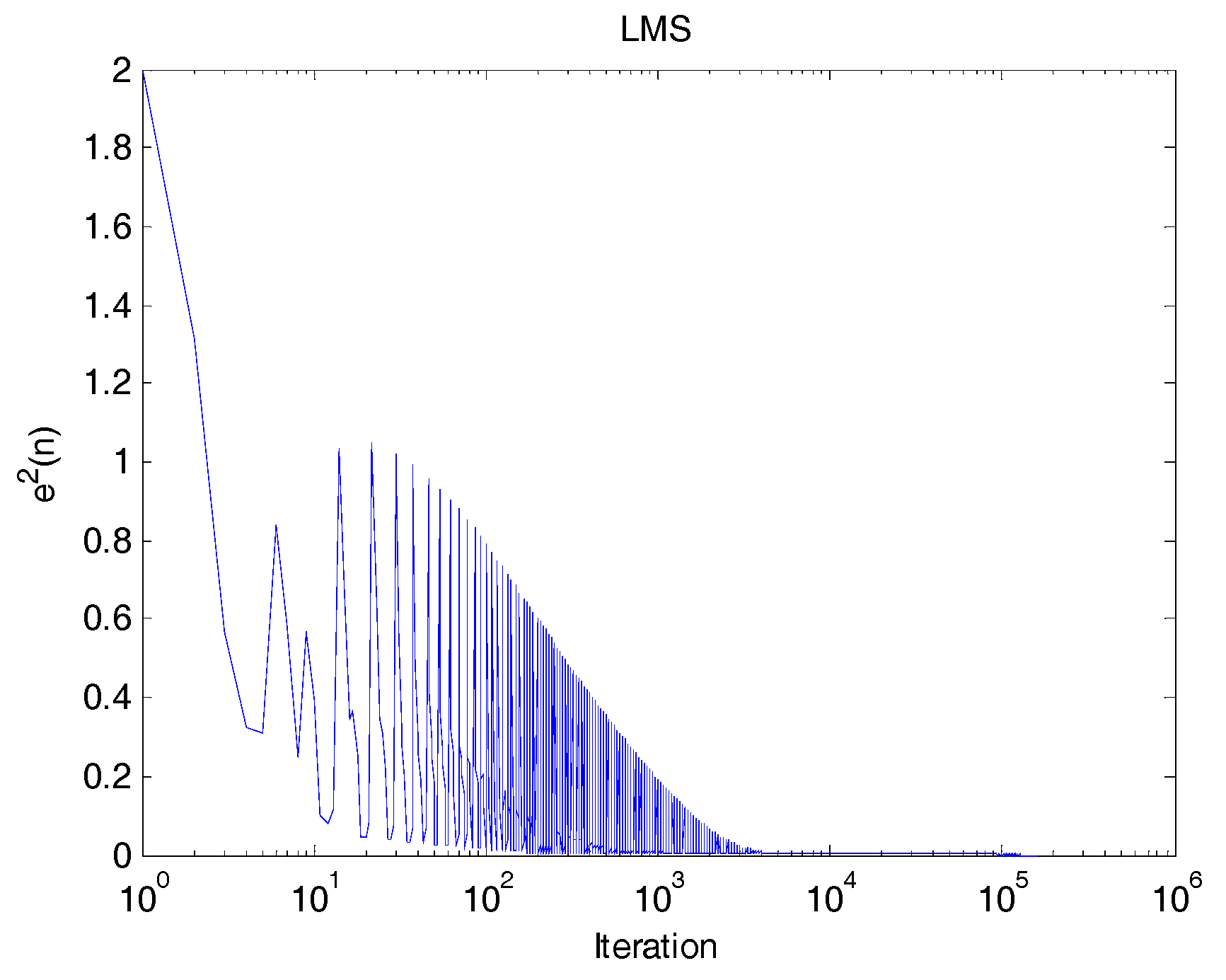
Figure 7, the combination of weighed detection points in the time domain and frequency are performed. These weights are calculated by adaptive LMS algorithm. In this way, the number of iterations is 100 thousand; the step is 0.2 and for training three signals as environmental noise and three signals as the target are used. Figure 18 shows learning curves of the LMS adaptive filter for the cases under test.
5. Discussion and Conclusions
In this paper, a novel algorithm for target detection in time and frequency domain is proposed. In order to compare, the results of this method are compared with three general and practical passive sonar detection methods as sonar equation [20], detection based on the DEMON and independent component analyze (ICA) [14], and target detection based on TPSW and neural networks [4] are expressed briefly in the following.
Sonar equation is the basic method for calculation detection threshold. The equation for determining the performance of passive sonar is , where SL is the source level, TL is the transmission loss, NL is the noise level, DI is the directivity index of the array (an approximation to the array gain), and DT is the detection threshold. In this paper, optimum DT is selected by ROC curve. Table 3 shows the values of parameters of sonar equation in the Persian Gulf.
In [14], for target detection, DEMON analysis is applied. DEMON algorithm is a narrow-band filter that reduces the ambient noises. Then, output signal are performed over the independent sources (ICA). The ICA provides a linear representation of non-Gaussian data, so that components are statistically independent, or as much independent as possible.
The detection method is described in [4]. In the preprocessing and feature extraction stage, TPSW algorithm is used to extract tonal features from the average power spectral density. In the classification stage, neural network classifiers are used to evaluate the classification results, inclusive of the hyper plane based Classifier-Multilayer Perceptron (MLP).
To compare proposed method with the three expressed methods same database is used. In this investigation, three categories of test data are considered. The first category includes vessels with small size and fast (e.g., barges), the second category includes medium vessels (e.g., cart), and third includes large vessels with low speed.
Acknowledgments
The authors are grateful to the Department of Electrical and Computer Engineering Birjand University for financial support. The authors thank the Noar Institute Research for experimental support. Finally, the authors would like to express their sincere gratitude to all of those who have offered selfless help during the course of this research.
Author Contributions
All authors (Hamed Komari Alaie, Hassan Farsi) contributed to the research work. Hamed Komari Alaie conceived and designed the prototype observation; Hassan Farsi performed the prototype tests and analyzed the data; Hamed Komari Alaie contributed analysis tools; and Hassan Farsi drafted the paper.
Conflicts of Interest
The authors declare no conflict of interest.
References
- Urick, R.J. Principles of Underwater Sound, 3rd ed.; McGraw-Hill: Seattle, WA, USA, 1983. [Google Scholar]
- Nielsen, R.O. Sonar Signal Processing; Artech House Inc.: Norwood, MA, USA, 1991. [Google Scholar]
- Dawe, R.L. Detection Threshold Modelling Explained; DSTO Aeronautical and Maritime Research Laboratory: Melbourne, Australia, 1997.
- Chen, C.F.; Lee, J.D.; Lin, M.C. Classification of Underwater Signals Using Neural Networks. Tamkang J. Sci. Eng. 2000, 3, 31–48. [Google Scholar]
- Abraham, D.A. Detection-Threshold Approximation for Non-Gaussian Backgrounds. IEEE J. Ocean. Eng. 2010, 35, 355–365. [Google Scholar] [CrossRef]
- Wakayama, C.Y.; Grimmett, D.J.; Zabinsky, Z.B. Forecasting Probability of Target Presence for Ping Control in Multistatic Sonar Networks using Detection and Tracking Models. In Proceedings of the 14th International Conference on Information Fusion, Chicago, IL, USA, 5–8 July 2011. [Google Scholar]
- Chung, K.W.; Sutin, A.; Sedunov, A.; Bruno, M. DEMON Acoustic Ship Signature Measurements in an Urban Harbor. Adv. Acoust. Vib. 2011, 2011. [Google Scholar] [CrossRef]
- Diamant, R. Closed Form Analysis of the Normalized Matched Filter with a Test Case for Detection of Underwater Acoustic Signals. IEEE Access 2016, 4, 8225–8235. [Google Scholar] [CrossRef]
- Xu, L.; Liu, C.; Yi, W.; Li, G.; Kong, L. A particle filter based track-before-detect procedure for towed passive array sonar system. In Proceedings of the 2017 IEEE Radar Conference, Seattle, WA, USA, 8–12 May 2017. [Google Scholar]
- Martino, J.C.D.; Haton, J.P.; Laporte, A. Lofargram line tracking by multistage decision. In Proceedings of the Speech, and Signal Processing, Minneapolis, MN, USA, 27–30 April 1993. [Google Scholar]
- Borowski, B.; Sutin, A.; Roh, H.S.; Bunin, B. Passive acoustic threat detection in estuarine environments. In Proceedings of the Optics and Photonics in Global Homeland Security IV, Orlando, FL, USA, 17–20 April 2008; Volume 6945. Aricle No. 694513. [Google Scholar]
- Zhao, Z.; Zhao, A.; Hui, J.; Hou, B.; Sotudeh, R.; Niu, F. A Frequency-Domain Adaptive Matched Filter for Active Sonar Detection. Sensors 2017, 17, 1565. [Google Scholar] [CrossRef] [PubMed]
- Zhang, L.; Wu, D.; Han, X.; Zhu, Z. Feature Extraction of Underwater Target Signal Using Mel Frequency Cepstrum Coefficients Based on Acoustic Vector Sensor. J. Sens. 2016, 2016. [Google Scholar] [CrossRef]
- De Moura, N.N.; De Seixas, J.M.; Ramos, R. Passive Sonar Signal Detection and Classification Based on Independent Component Analysis. In Sonar Systems; INTECH: Rijeka, Croatia, 2011; pp. 93–104. [Google Scholar]
- Gupta, A.S.; Kirsteins, I. Sonar target detection and classification against non-stationary interference using dynamic time-frequency localization. In Proceedings of the Signals, Systems and Computers, 2013 Asilomar Conference on, Pacific Grove, CA, USA, 3–6 November 2013. [Google Scholar]
- Ciuonzo, D.; Willett, P.K.; Bar-Shalom, Y. Tracking the tracker from its passive sonar ML-PDA estimates. IEEE Trans. Aerosp. Electron. Syst. 2014, 50, 573–590. [Google Scholar] [CrossRef]
- Kirubarajan, T.; Bar-Shalom, Y. Low observable target motion analysis using amplitude information. IEEE Trans. Aerosp. Electron. Syst. 1996, 32, 1367–1384. [Google Scholar] [CrossRef]
- Johann, P. Parametric Statistical Theory; Walter de Gruyter: Berlin, German, 1994. [Google Scholar]
- Ciuonzo, D.; De Maio, A.; Rossi, P.S. A Systematic Framework for Composite Hypothesis Testing of Independent Bernoulli Trials. IEEE Signal Process. Lett. 2015, 22, 1249–1253. [Google Scholar] [CrossRef]
- Ekimov, A.; Sabatier, J.M. Human detection range by active Doppler and passive ultrasonic methods. In Proceedings of the Sensors, and Command, Control, Communications, and Intelligence (C3I) Technologies for Homeland Security and Homeland Defense VII, Orlando, FL, USA, 5–9 April 2008; Proceedings of SPIE 6943. SPIE: Bellingham, WA, USA, 2008. [Google Scholar]
Figure 1.
Basic of target detection in passive sonar.

Figure 2.
Persian Gulf territory.
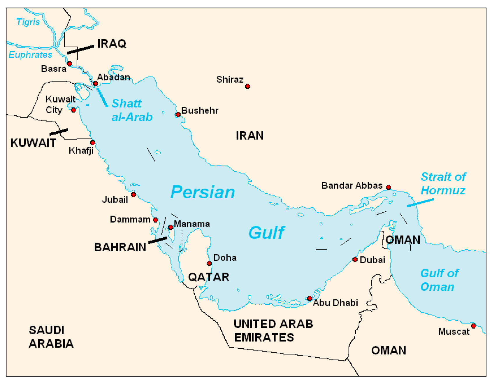
Figure 3.
Block diagram of proposed method.

Figure 4.
Center of noise and target cluster. (a) Large center is selected as detection point and (b) large center is selected as detection point incorrectly.
Figure 4.
Center of noise and target cluster. (a) Large center is selected as detection point and (b) large center is selected as detection point incorrectly.
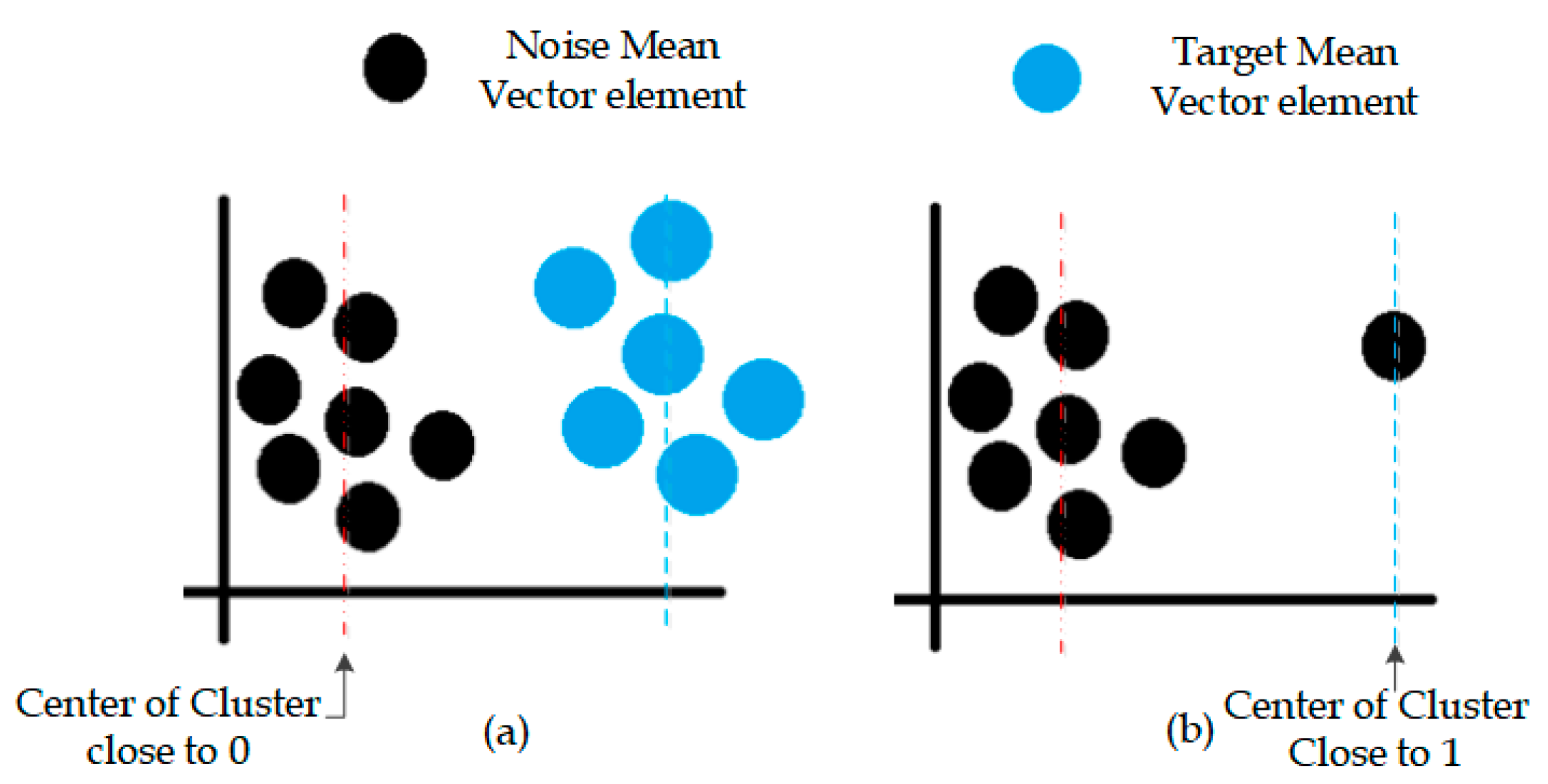
Figure 5.
How to calculate detection point in time domain.

Figure 6.
How calculate detection point in frequency domain.
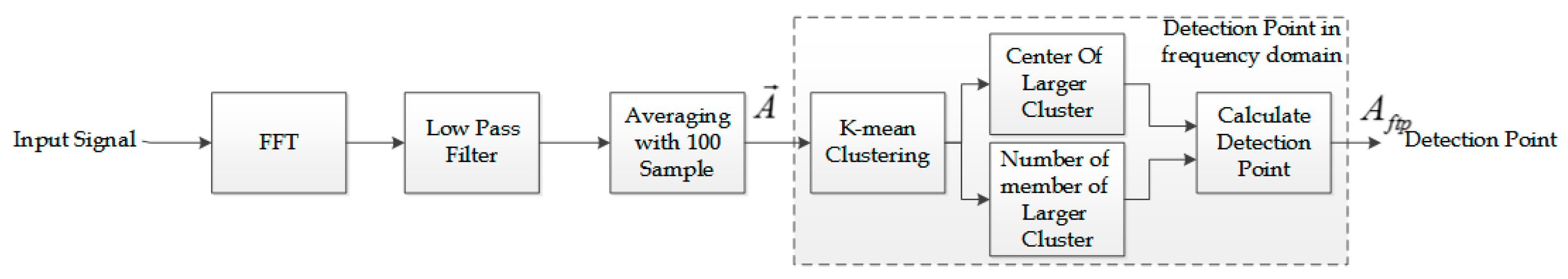
Figure 7.
The fusion of detection points in both time and frequency domains.

Figure 8.
Propeller sound of a commercial vessel with sampling rate 44 kHz.

Figure 9.
Sample of ambient noise with sampling rate 44 kHz.
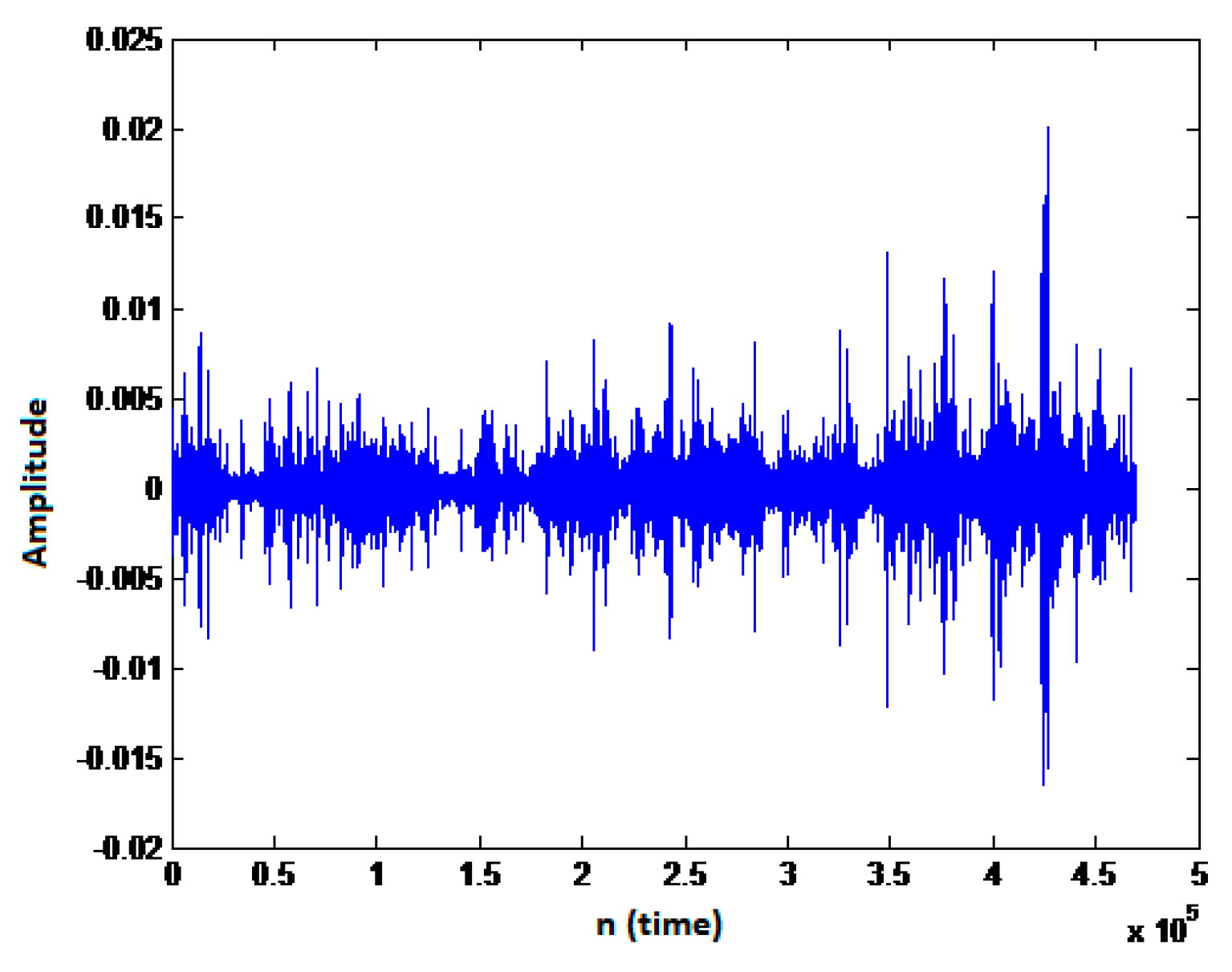
Figure 10.
Sample of the mixed sounds (ambient noise and propeller sound).
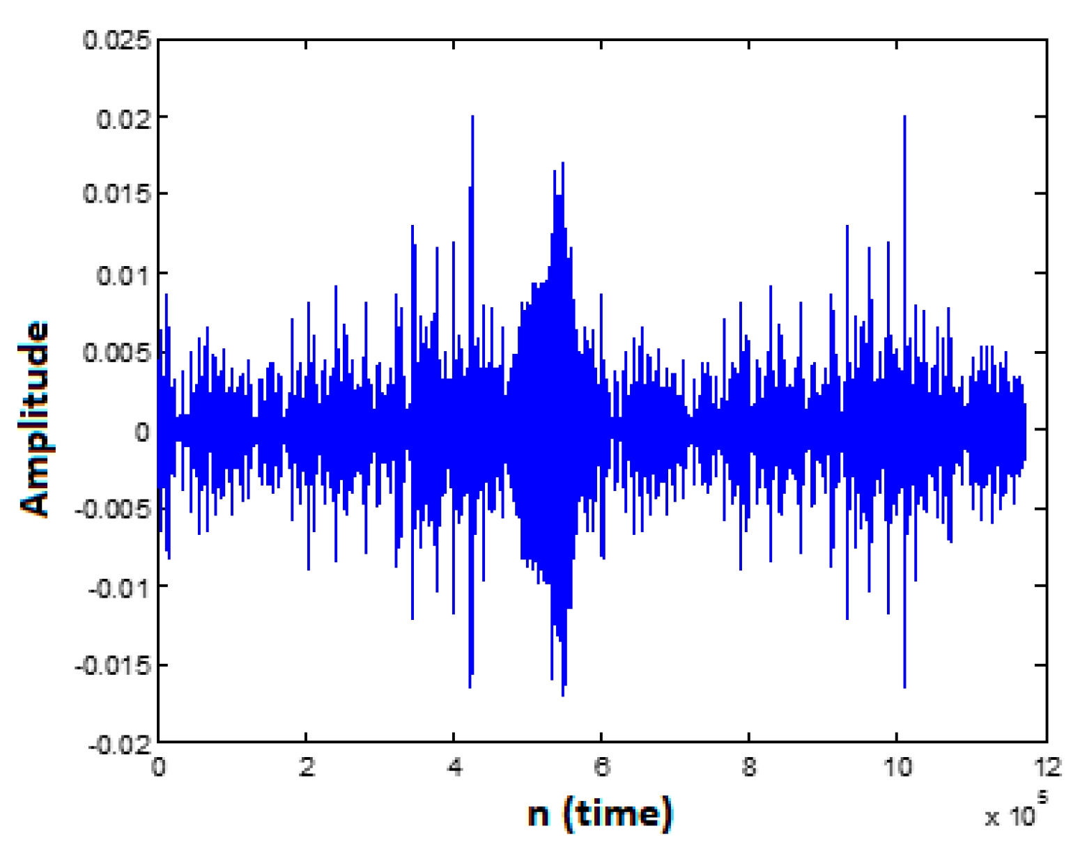
Figure 11.
Bayesian classifier output, in sample of 50 thousand and 100 thousand real target is present (red ellipse).
Figure 11.
Bayesian classifier output, in sample of 50 thousand and 100 thousand real target is present (red ellipse).
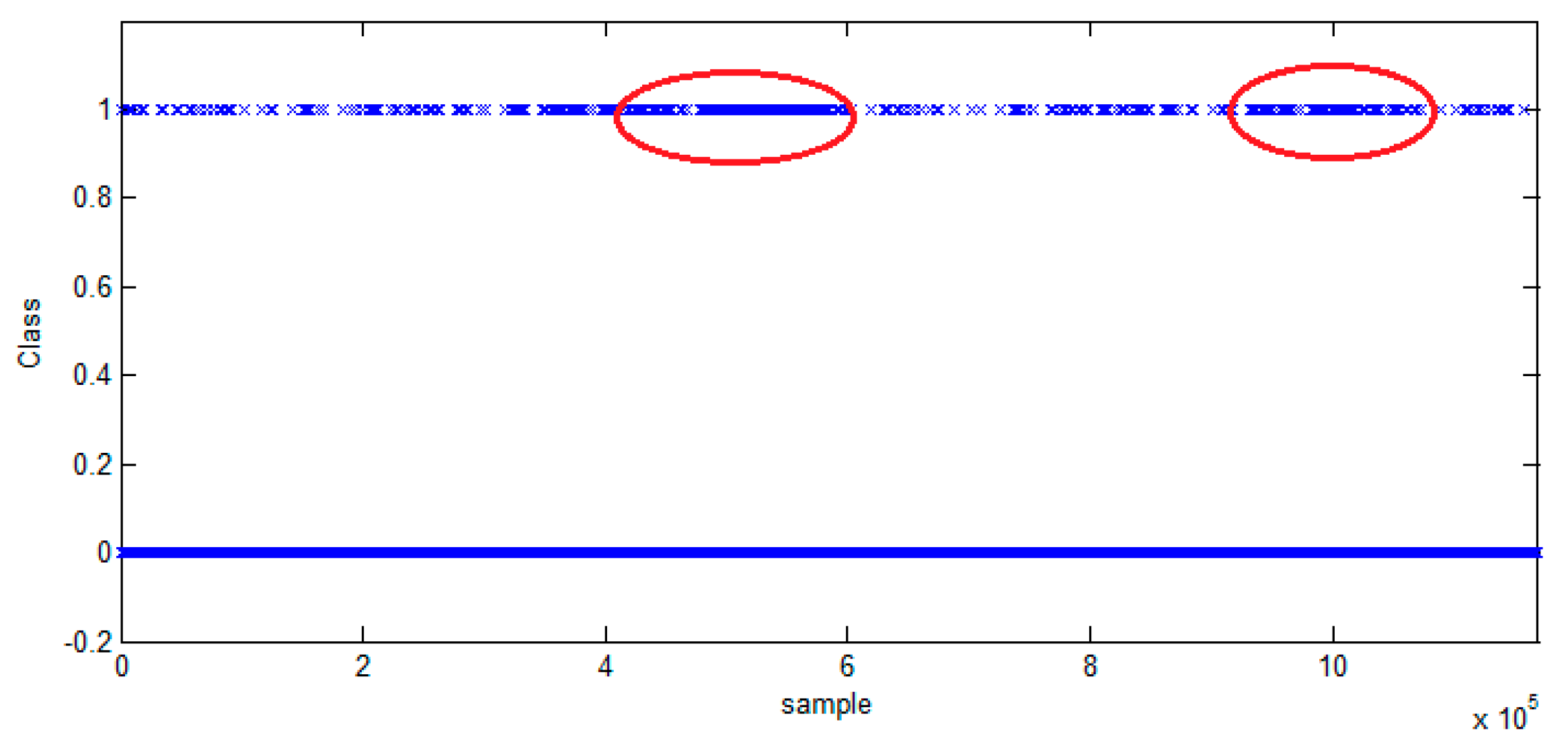
Figure 12.
Average vector , detection point is increased after 10 samples.
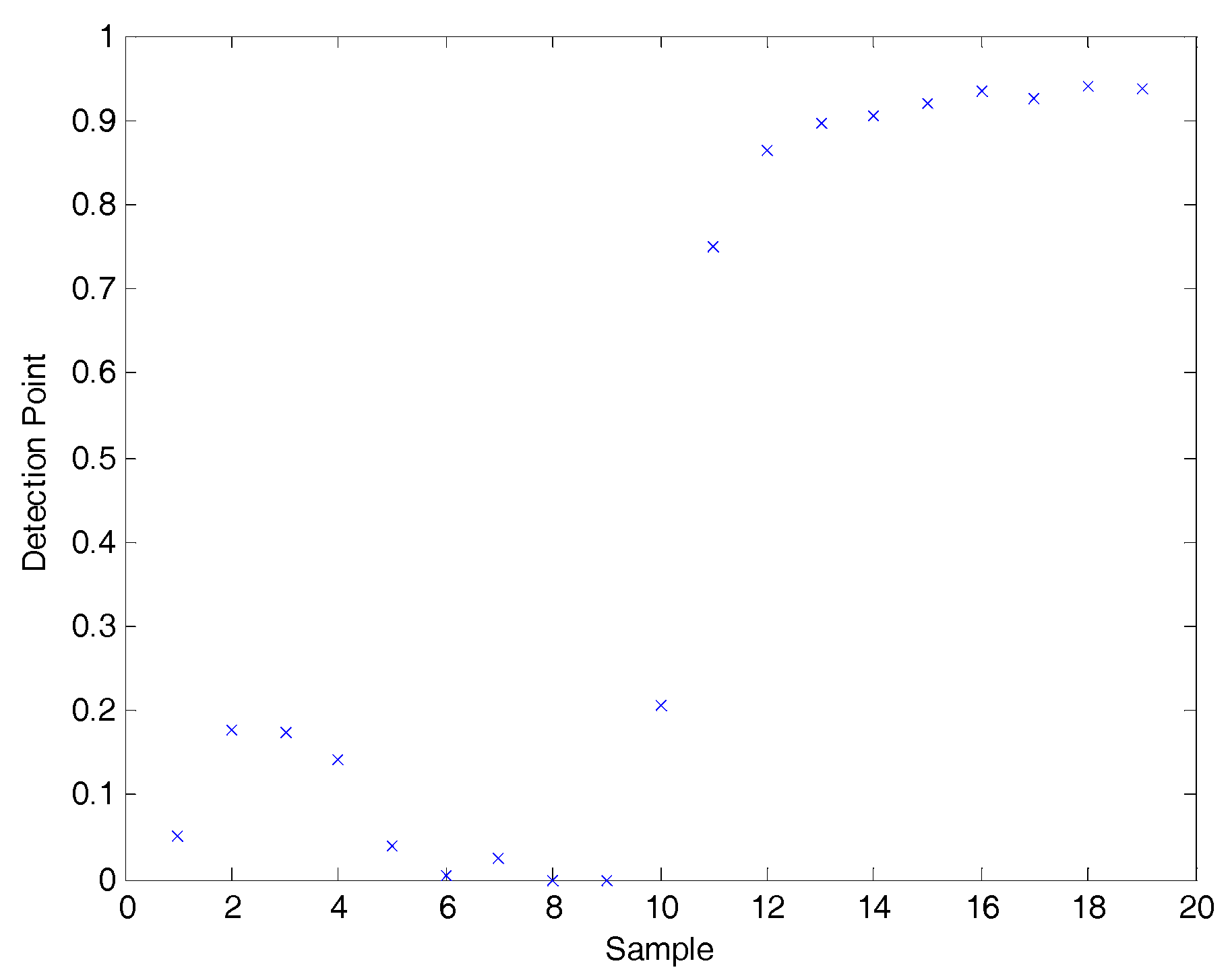
Figure 13.
Results of K-means (K = 2), dots shown elements of the first cluster, crosses shown elements of the second cluster and the hollow circles are the cluster center.
Figure 13.
Results of K-means (K = 2), dots shown elements of the first cluster, crosses shown elements of the second cluster and the hollow circles are the cluster center.

Figure 14.
Vector for two target signals (13 and 14) and two ambient noise signals (15 and 16) in the time domain.
Figure 14.
Vector for two target signals (13 and 14) and two ambient noise signals (15 and 16) in the time domain.

Figure 15.
Mean vector .

Figure 16.
Vector for two target signals (13 and 14) and two ambient noise (15 and 16).

Figure 17.
Average of 20 (m = 20) sequences for 19 test signals (1 to 14 are target signals and 15 to 19 are ambient noise signals).
Figure 17.
Average of 20 (m = 20) sequences for 19 test signals (1 to 14 are target signals and 15 to 19 are ambient noise signals).

Figure 18.
Learning curves of the Least Mean Square (LMS) adaptive filter for the cases under test.

Figure 19.
DP for 19 test signals (1 to 14 are the target signals and 15 to 17 are only ambient noise).
Figure 19.
DP for 19 test signals (1 to 14 are the target signals and 15 to 17 are only ambient noise).
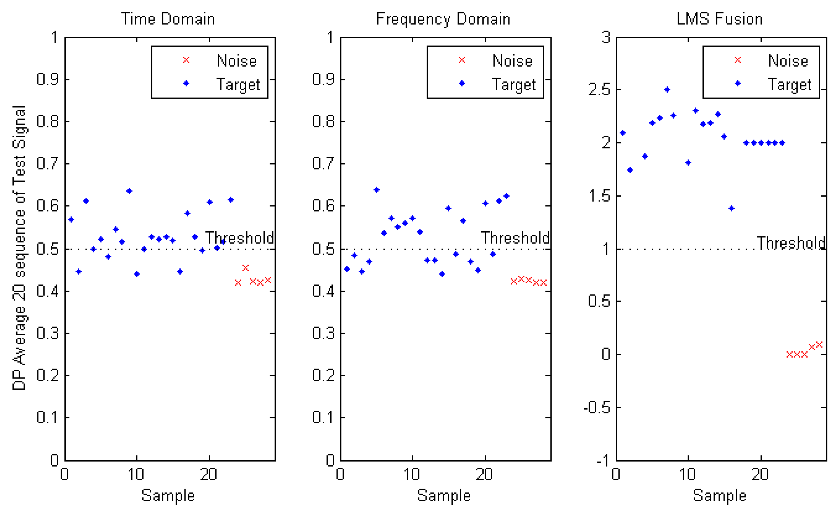
Figure 20.
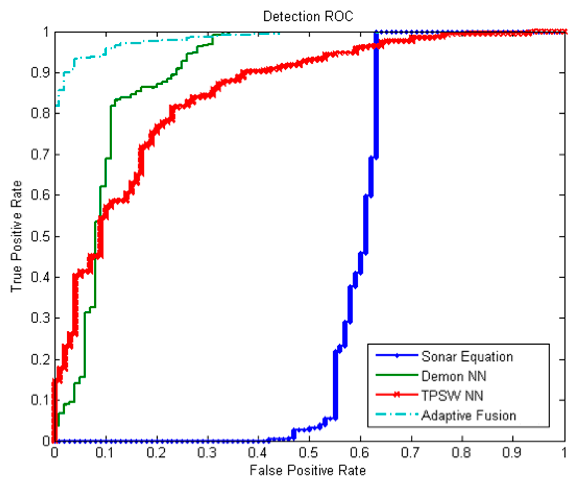
Receiving Operating Characteristics (ROC) Experimental results for target detection. TPSW NN: Two-Pass Split-Windows Neural Network; DEMON: Detection Envelope Modulation on Noise Neural Network.
Figure 20.
Receiving Operating Characteristics (ROC) Experimental results for target detection. TPSW NN: Two-Pass Split-Windows Neural Network; DEMON: Detection Envelope Modulation on Noise Neural Network.


Table 1.
Detection point of 19 test signals in a specific sequence in the time domain.
| No. | Type | |
|---|---|---|
| 1 | Ship Engine 1 | 0.83 |
| 2 | Ship Propeller 1 | 0.62 |
| 3 | Ship 1 | 0.39 |
| 4 | Ship Engine 2 | 0.61 |
| 5 | Ship 2 | 0.59 |
| 6 | Ship Engine 3 | 0.6 |
| 7 | Ship Engine 4 | 0.5 |
| 8 | Ship Engine 5 | 0.68 |
| 9 | Ship Engine 6 | 0.82 |
| 10 | Ship Propeller 2 | 0.21 |
| 11 | Ship Engine 7 | 0.46 |
| 12 | Ship Engine 8 | 0.53 |
| 13 | Ship Engine 9 | 0.7 |
| 14 | Ship Engine 10 | 0.58 |
| 15 | Ambient Noise 1 | 0.43 |
| 16 | Ambient Noise 2 | 0.39 |
| 17 | Ambient Noise 3 | 0.37 |
| 18 | Ambient Noise 4 | 0.38 |
| 19 | Ambient Noise 5 | 0.26 |
Table 2.
Detection points for 19 test input signals in a specific sequence in the frequency domain.
| No. | Type | |
|---|---|---|
| 1 | Ship Engine 1 | 0.46 |
| 2 | Ship Propeller 1 | 0.63 |
| 3 | Ship 1 | 0.65 |
| 4 | Ship Engine 2 | 0.47 |
| 5 | Ship 2 | 0.63 |
| 6 | Ship Engine 3 | 0.83 |
| 7 | Ship Engine 4 | 0.43 |
| 8 | Ship Engine 5 | 0.48 |
| 9 | Ship Engine 6 | 0.49 |
| 10 | Ship Propeller 2 | 0.57 |
| 11 | Ship Engine 7 | 0.53 |
| 12 | Ship Engine 8 | 0.61 |
| 13 | Ship Engine 9 | 0.43 |
| 14 | Ship Engine 10 | 0.38 |
| 15 | Ambient Noise 1 | 0.37 |
| 16 | Ambient Noise 2 | 0.36 |
| 17 | Ambient Noise 3 | 0.21 |
| 18 | Ambient Noise 4 | 0.32 |
| 19 | Ambient Noise 5 | 0.02 |
Table 3.
Value of parameters of sonar equation in the Persian Gulf. DI: directivity index; NL: noise level; TL: transmission loss; SL: source level.
Table 3.
Value of parameters of sonar equation in the Persian Gulf. DI: directivity index; NL: noise level; TL: transmission loss; SL: source level.
| Parameter | DI | NL | TL | SL |
|---|---|---|---|---|
| Value (dB) | 200 | 19.02 | 90 | 31.9 |
Table 4.
True detection rate. TPSW NN: Two-Pass Split-Windows Neural Network; DEMON: Detection Envelope Modulation on Noise.
Table 4.
True detection rate. TPSW NN: Two-Pass Split-Windows Neural Network; DEMON: Detection Envelope Modulation on Noise.
| Detection Method | Proposed Method (Adaptive Fusion) | The Method Described in [4] (TPSW NN) | The Method Described in [14] (DEMON) | The Method Described in [20] (Sonar Equation) |
|---|---|---|---|---|
| Database | ||||
| First category | 81.20% | 60.35% | 51.12% | 25.36% |
| Second category | 73.41% | 44.26% | 48.20% | 23.85% |
| Third category | 94.32% | 63.57% | 69.12% | 46.35% |
| Total | 85.40% | 58.75% | 61.27% | 35.71% |
© 2018 by the authors. Licensee MDPI, Basel, Switzerland. This article is an open access article distributed under the terms and conditions of the Creative Commons Attribution (CC BY) license (http://creativecommons.org/licenses/by/4.0/).
Share and Cite
MDPI and ACS Style
Komari Alaie, H.; Farsi, H. Passive Sonar Target Detection Using Statistical Classifier and Adaptive Threshold. Appl. Sci. 2018, 8, 61. https://doi.org/10.3390/app8010061
AMA Style
Komari Alaie H, Farsi H. Passive Sonar Target Detection Using Statistical Classifier and Adaptive Threshold. Applied Sciences. 2018; 8(1):61. https://doi.org/10.3390/app8010061
Chicago/Turabian StyleKomari Alaie, Hamed, and Hassan Farsi. 2018. "Passive Sonar Target Detection Using Statistical Classifier and Adaptive Threshold" Applied Sciences 8, no. 1: 61. https://doi.org/10.3390/app8010061
Note that from the first issue of 2016, this journal uses article numbers instead of page numbers. See further details here.