1. Introduction
In the design and optimization of many applications based on latent heat, be it storages or thermal regulations for instance, the need for a precise determination of the properties of the PCM has critically increased. Usually, this demand is fulfilled in two manners: either the determination of the temperature(s) connected to the phase change and the corresponding latent heat(s), or the determination of the enthalpy function. In this latter case, the influence of the pressure on this thermodynamical function is generally neglected (applications under pressure being very rare) and only the dependency on the temperature and on the relative local liquid (or solid) mass fraction—during the phase transition—are required. In summary, the goal is to determine the correct formulation of the specific enthalpy
h of the involved material:
where
i represent the various substances, which can be pure or in solution (solvent in majority or various solutes), and
the corresponding mass fractions with
= liquid (
L) or solid (
S).
Keeping in mind these two types of characterization, the aim of the present paper is to challenge the usual approaches encountered when tackling such an issue:
In the first case, where only the global values for the characteristic data (temperature(s) and latent heat(s)) are searched for, the main methods are based on a graphical exploitation of the DSC curve. Thus, by looking specific points of the thermogram, as for instance the onset temperature, one tries to obtain a correct determination of the temperature(s) which can be representative of the phase change. Then, by defining an integration method, the corresponding latent heat(s) could be obtained.
In the second case, where the complete mathematical expression of the enthalpy is searched for, the main method often relies on the so-called equivalent heat capacity method that assumes that the thermogram can be interpreted as the derivative of the enthalpy. Thus, a direct integration of the DSC curve, favoring low heating rates, should permit to go back up to the enthalpy function.
The main conclusions of the present study are that both approaches are, in the best cases, mainly approximate solutions. Moreover, in many situations, they could be misleading and can furnish a wrong characterization incompatible with thermodynamics. These conclusions principally stream from an incomplete view from the physical phenomenon involved during the phase transition when analyzing the DSC curve. Indeed, the thermal transfers are generally considered only at the boundaries of the sample, i.e., with the apparatus, however the thermal transfers inside the sample are completely neglected although a thermal gradient is known to exist in such a case [
1,
2,
3]. Another common reason for this incorrect estimation often lies in the expression of the enthalpy, which does not correspond to the real behavior of the sample. Thus, in almost all cases, all materials are analyzed as if they were pure substances despite their scarce availability (even with laboratory grade materials—without speaking of technical grades).
In the present paper, several models will be presented in order to reproduce the behavior of various materials. The cornerstone of this approach is to always rely on the basic laws of thermodynamics. It is then shown that every usual thermograms can thus be easily reproduced and analyzed, and that no need for artefacts or "extra-thermodynamics" assumptions is required.
The first part of this paper will recall the usual impediment associated with the classical analysis. Then, in
Section 3 the present approach is developped: by coupling numerical simulations with experimental measurements, it is proposed a painstaking analysis of the various shapes of the DSC curves. The onus of our method is given in
Section 4, together with practical advices for experimenters to further improve the analysis of experiments. Finally, an extension and a comparison with the other possible approaches are furnished in
Section 5. Besides, a specific section devoted to the treatment and interpretation of supercooling (delay at the liquid crystallization) is added in
Section 6. Eventually, a conclusion is proposed.
2. Usual Caveats
In the practice of calorimetric analysis, a generally accepted assumption is to consider the thermogram as an accurate image of the intrinsic energy properties of the sample expressed by the equation of state of the material. In this context of analysis, it is common to make recommendations as to the speeds and masses to be used. Indeed, these parameters specific to the method have a real effect on the shape of the thermogram. This leads to consider the plate temperature
as representative to the sample temperature [
4,
5,
6].
However, we have already demonstrated, besides the smallness of the sample (about 10
), that the model considering an uniform temperature field [
4,
5,
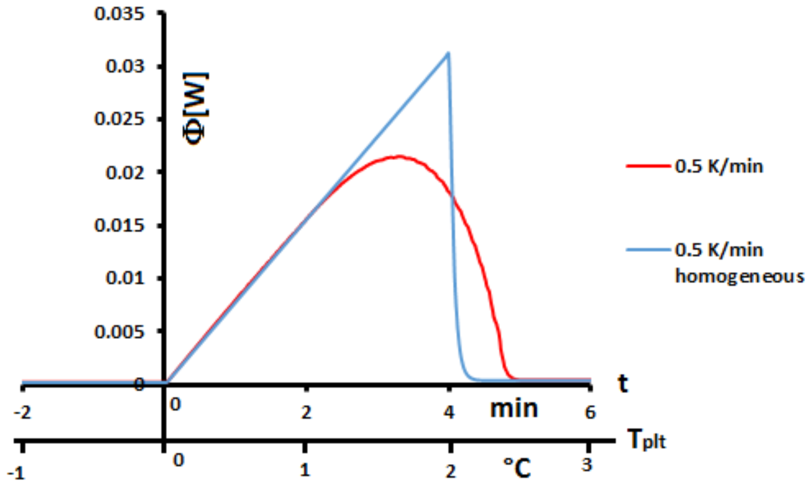
6], is not correct. For example, if we compare in
Figure 1 the thermograms (DSC curves) with this assumption and an experimental one, even during a melting at 0.5 K/min (reasonnable limit of our calorimeter) there exists a large discrepancy between the two thermograms and the enlargement of the peak indicates the effects of the internal heat transfers. So, it is not possible to consider the sample as homogeneous.
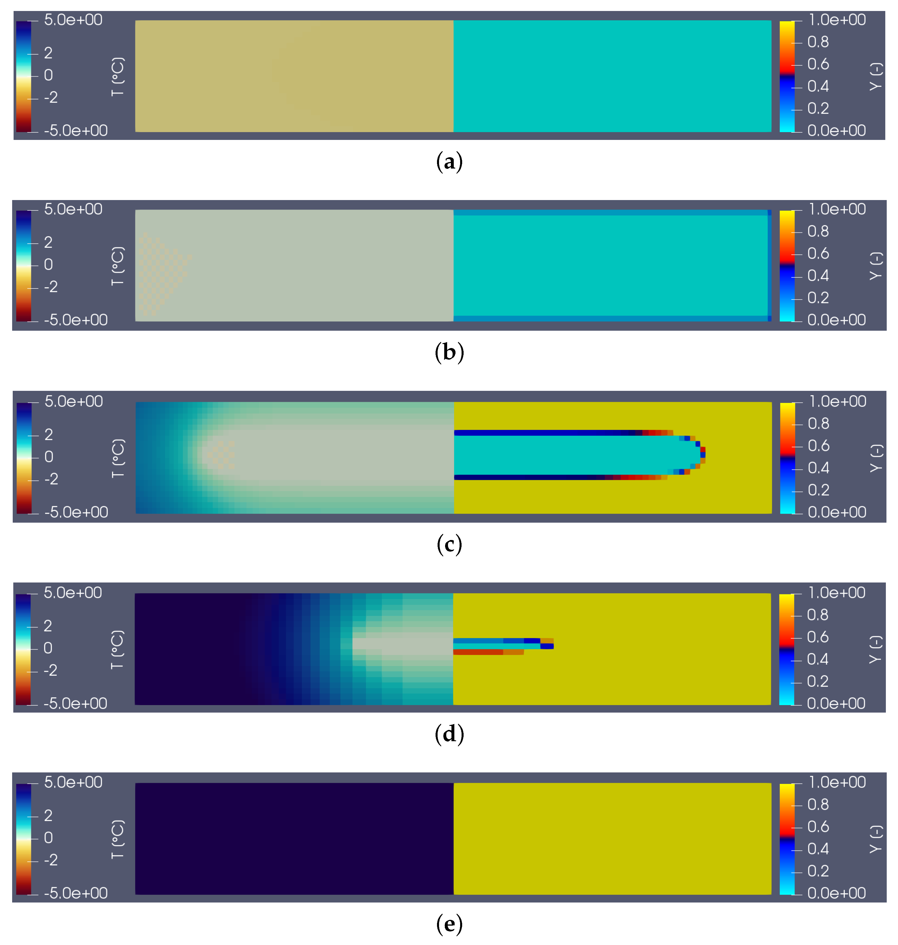
To detail the thermal phenomena whose thermogram of
Figure 2 is the description,
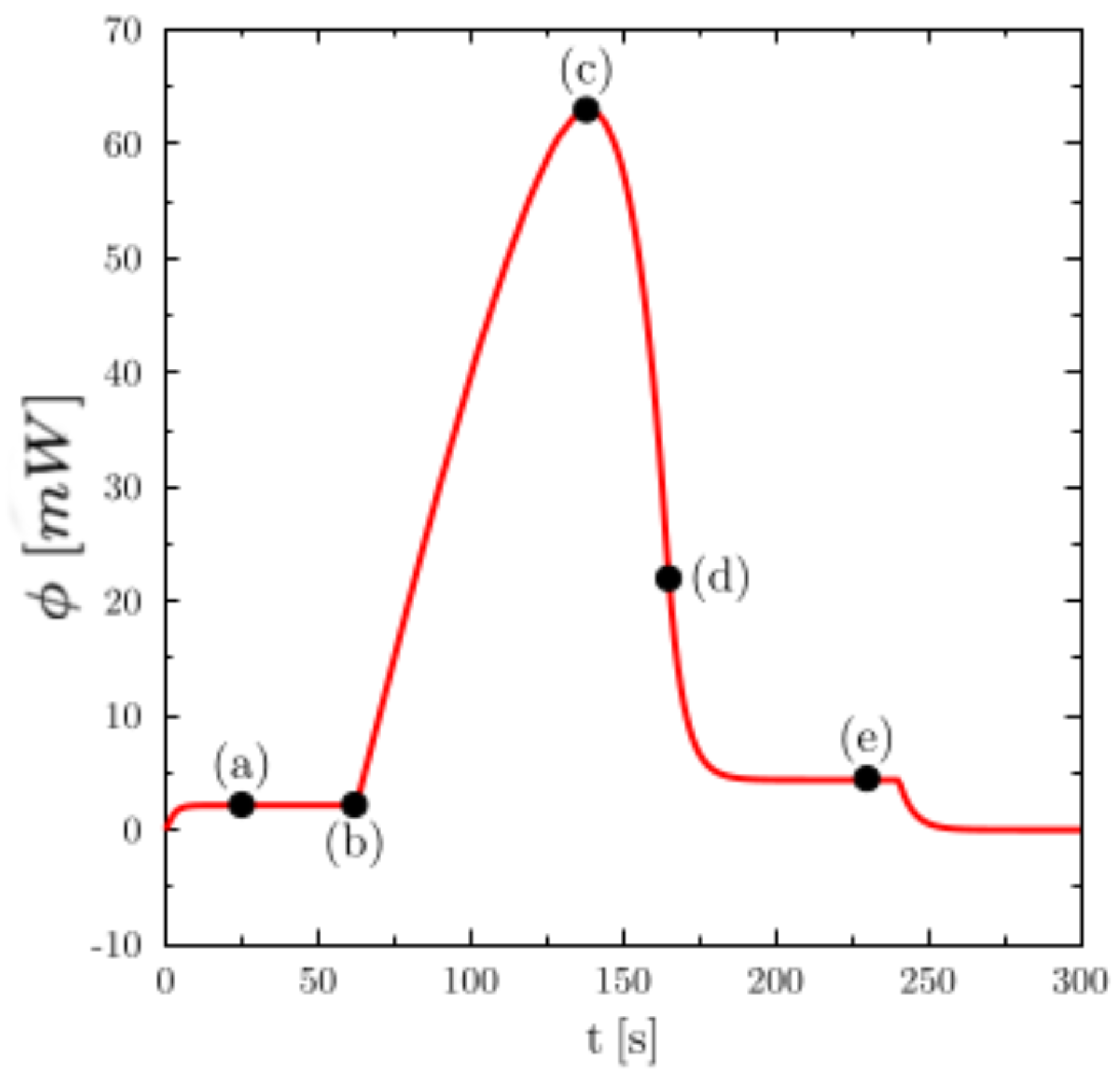
Figure 3 shows the temperature (on the left) and liquid fraction (on the right) fields in the sample (water) during heating. There are five characteristic states (see the corresponding instants on the corresponding thermogram hereafter): in (a), the material is in the solid state (
) and the temperature is almost homogeneous. At point (b) the melting begins (
close to the walls). The still solid zone is homogeneous and at melting temperature. Point (c) corresponds to the time when the heat flux measured by the calorimeter is maximum. Note that this state does not correspond to any particular change in field structure. Point (d) corresponds to the end of the melting and thus the disappearance of the last solid zone. This moment always corresponds to the inflection point observed on the thermogram. The system then returns to equilibrium (liquid) with an almost homogeneous temperature (linear zone of the point (e)).
When calorimetry is used for routine analyses, we observe, on the same product, different thermograms following the heating rates or the masses of the samples, and the
Figure 3 permits a qualitative explanation without a change in the thermodynamic properties of the material can be questioned. However, these influences of mass and velocity may suggest, to certain authors, that the thermal characteristics of the material depends on mass and velocity (amplitude and sign). This is obviously an aberration that is simply forbidden by the laws of thermodynamics, the enthalpy
h being a state function.
The main key to right-understand the effect of mass and velocity lies in abandoning the previously homogeneous assumption considering the thermogram as an image of the intrinsic thermal behavior of the sample as a whole. It will be demonstrated that this new key of analysis allows to naturally explain the effects of the mass and the heating/cooling rate on the DSC curve.
The phenomenon of hysteresis is sometimes evoked to explain the difference in the shape of the thermogram (other than the up/down orientation) between cooling and heating. Some people try to explain it by considering two “behaviors” for the material according to whether it is heated or cooled, which is obviously once again a thermodynamic aberration. This phenomenon is explicitly and rigorously explained only by considering heat transfers within the sample.
Another very important consequence concerns the temperature of the sample that can’t be considered isothermal yet. One can no longer define “the” (unique) temperature of the sample and consequently, and by the way, one can no longer associate a temperature with a flux event observed on the thermogram. Similarly, since it is not possible to define “the” (unique) temperature of the sample, how to define a relation with the temperature of the plate imposed by the measuring instrument?
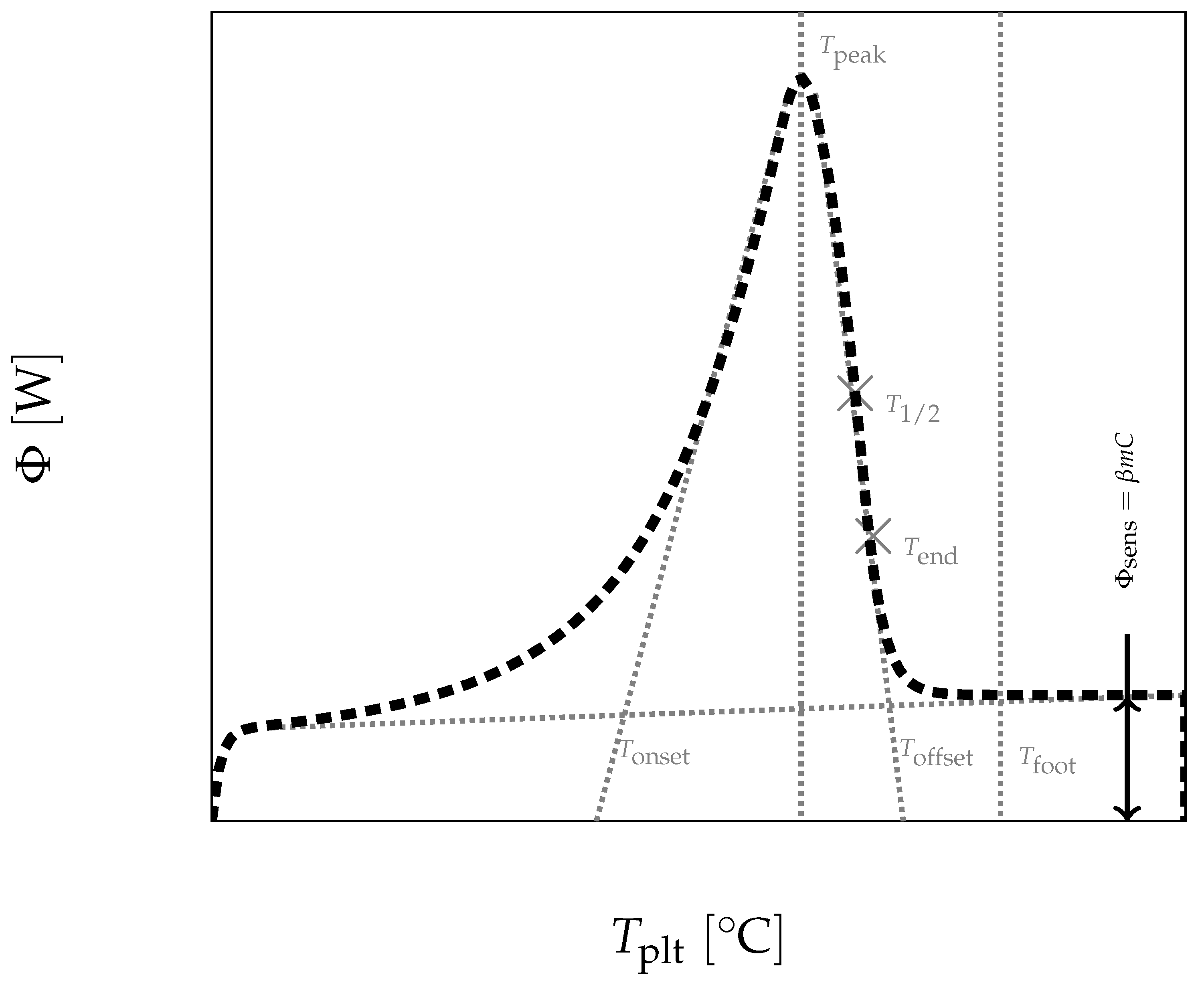
In
Figure 4, we present a thermogram with the different lines permitting to determine the temperatures generally considered as characteristic of the phase transformations e.g., the onset temperature
, the temperature of the top of the peak
, the temperature at the half height of the peak
, the temperature of the end of transformation
, the offset temperature
or the temperature of the end of the peak
. We will indicate if these temperatures have a real significance or not.
3. Methodology
As depicted in
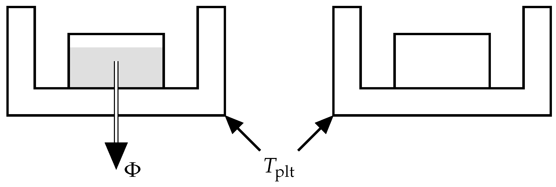
Figure 5, DSC is a technique consisting in measuring a heat-flow rate when the plates containing the reference and sample cells have an imposed temperature [
4]. The device maintains this temperature equality by heating the two cells in a differential way. The difference in power dissipation to the measurement cell and the reference cell eliminates the influence of the container and thus determines the net heat flux
exchanged with the sample. It should be noted that the sign convention may change depending on the manufacturer. For our experiments we use the convention of our calorimeter where the endothermic phenomena are represented towards positive ordinates.
Thus, the DSC curve records the variation of the heat-flow rate during time, i.e., when the plate temperature is evolving with time.
As a rule of thumb, the thermal request is based on the setting of a heating/cooling curve generally due to a linear variation of the temperature of the plate
:
where
in case of heating and
in case of cooling and
the temperature of the plate at
.
With respect to the previous remarks, when simulating the DSC experiment [
7,
8], one has to consider the heat equation inside the sample:
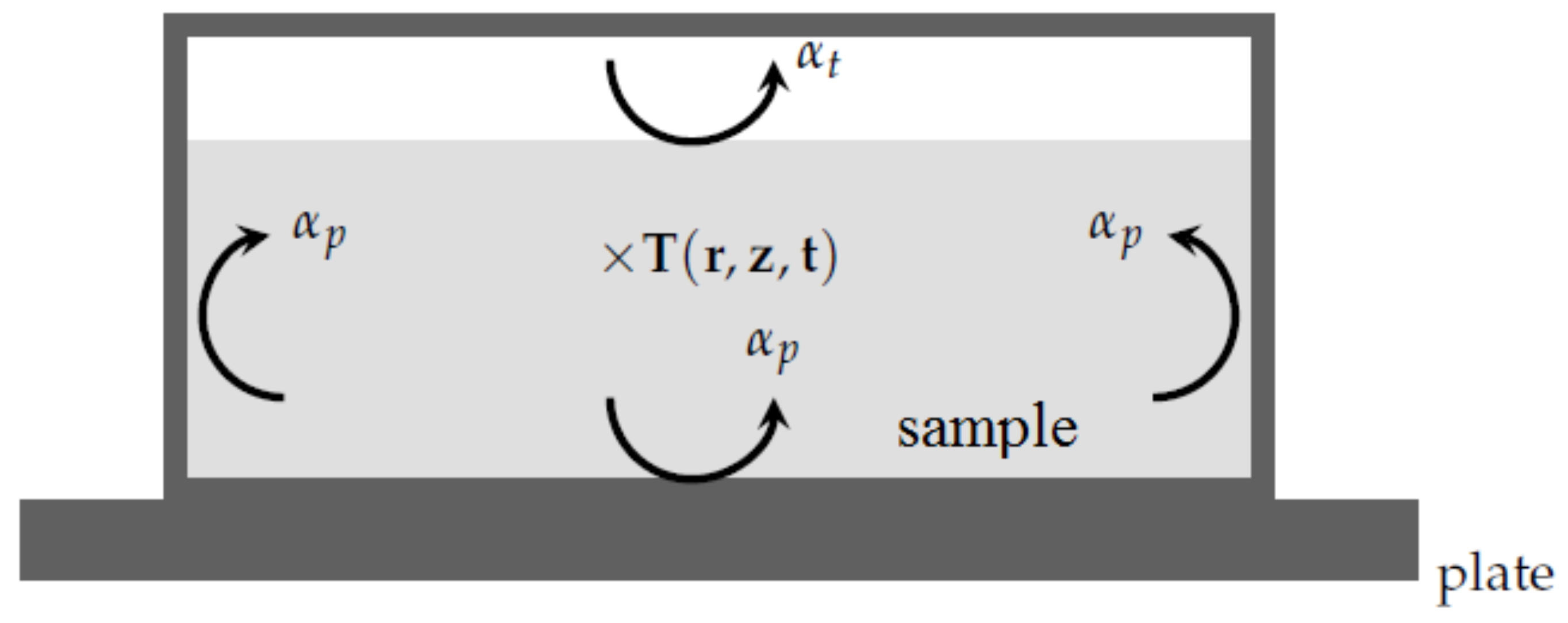
From a practical point of view with the PCM in question with a relatively low thermal conductivity, the temperature of the metallic pan equals the temperature of the plate. Therefore, the boundary conditions corresponding to the present system are (see
Figure 6):
where
or
according to the location of the interface
i are the heat transfer coefficients between the sample and the metallic pan.
Thus, when adding the various contributions for each boundary, the total heat flow rate
can be computed at every instant:
Finally, it means that if one incorporates the proper form for the enthalpy function in Equation (
3), then the response of the sample to the thermal stress Equation (
2) can be calculated thanks to the sum Equation (
5).
From a numerical point of view, this has been done here using a finite volume method with an explicit temporal integration and a first-order flux scheme on a structured mesh.
4. Results
Through the study of the numerical thermogram obtained by considering various enthalpy functions, i.e., different types of materials (pure substances, mixtures, etc.), the graphical analysis of the DSC curve are going to be challenged so as to determine their rightness, and when pertinent, their accuracy.
We first present an analysis of the phase transformation of a pure substance, followed by the study of the binary solutions. The results are used in the case of PCMs with impurities which present particular difficulties. The study is extended to binaries with solid solutions.
4.1. Pure Substances
4.1.1. Presentation
Although the pure substances and their characterization do not raise any difficulties, this section will highlight how the experimental thermogram could easily be erroneously interpreted when one tries to analyze it. The main goal here is to underline the nature of the usual errors and misunderstandings to further help the experimenters, specifically when considering non-pure substances that will be encountered in the following sections.
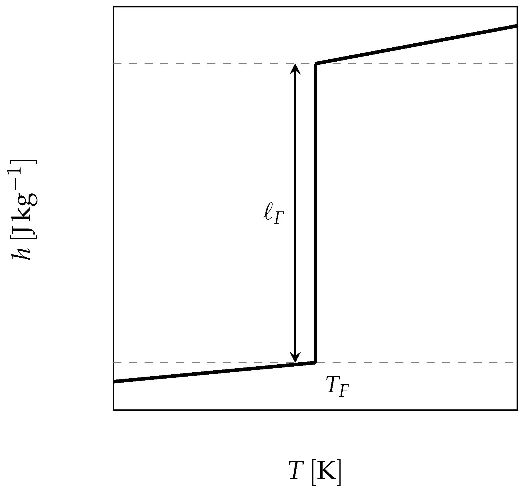
The starting point is thus the use of the enthalpy function for a pure substance, which undergoes its phase change at a constant temperature and presents a sharp discontinuity (as depicted in
Figure 7 and given by Equation (
6)), to solve the energy balance Equation (
3).
where
is the mass fraction of the liquid,
and
the specific heat of the liquid and the solid respectively and
the latent heat of melting.
n.b.: the reference state has been chosen at in solid state.
Following the procedure described hereinbefore, the heat flux can be reconstructed from relations Equations (
4) and (
5). Specifying that the programmed temperature for the calorimeter’s plate Equation (
2) is given by:
one can plot the thermogram as represented in
Figure 8.
Once again, one can notice that the thermogram does present a certain width despite the fact that melting occurs at a strictly constant temperature . Inversely, this implies logically that this width is not representative of a temperature range for the phase transition.
As highlighted in
Figure 2, the melting occurs first on the wall at the instant
where
. Then, when further increasing
, the phase change, located at the solid/liquid interface (first at the inner of the cell), does remain at the constant temperature
. In other words, there is an increase of the plate’s temperature whereas the phase transition interface and the solid part are still at the fusion temperature
. It is thus straightforward to conclude that
cannot be anymore representative of the sample’s behavior during the phase transition. Eventually, the melting is achieved when the last particle of solid disappears at time
, for a temperature
higher than
. At that moment, the strongest difference of temperatures in the cell is attained, with the last appeared liquid droplet being at
whereas the liquid next to the wall is at
. Once again, the fact that during the phase transition (occurring at the constant temperature
), the temperature of the plate evolves from
to
is in no way a proof that phase change arises on the same temperature range.
Finally, one remark is to be done that will have two main important consequences: as we precise later, only the left foot of the peak is representative of a physical characteristic (here, the beginning of the phase change). This implies that neither the peak temperature nor the offset temperature defined in
Figure 4 have any significant meanings. Besides, it has been shown that the end of the fusion of the last solid particle occurs at
, which corresponds to an inflexion point of the descending part of the curve (see
Figure 8). Moreover, the temperature
corresponds to the moment when there is no more temperature gradient in the liquid sample which is then thermally homogeneous. Before
and beyond
we will speak of a sensible zone with a flow rate
.
4.1.2. Discussion
To briefly summarize, the thermogram is representative of the phase change only if one considers the temporal evolution of the heat-flow rate and not the temperature of the plate. Indeed, inside the cell, since the phase change occurs on the interface which evolves with a constant temperature then, at no moment there exists a particle melting at a temperature different from .
We propose now to show the usual analysis, and to explain the implying behavior, so as to evaluate the various approaches, keeping in mind that the final goal is to determine the best ways for experimenters to analyze the thermograms.
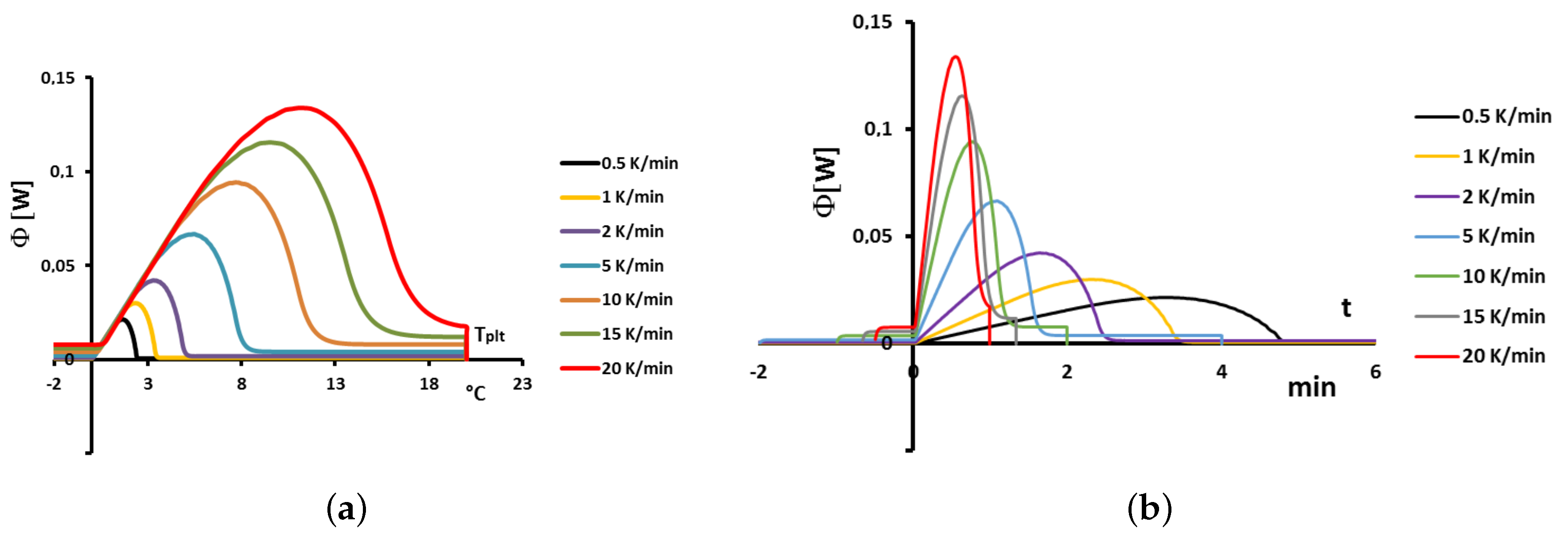
4.1.3. Influence of the Heating Rate
A
sample of water is tested at several heating rates
ranging from
to
. The corresponding thermograms are shown in
Figure 9 using either the plate’s temperature or the time for the abscissa coordinate.
Although the phase transition occurs at the same temperature in each case, the obtained thermogram is strongly dependent on the heating rate. However, this does not mean that the phase change is spread on a temperature range but only that it takes a longer time to proceed the entire fusion, i.e., a required duration for the interface to go through all the sample.
For the highest heating rates, the duration of the experiment is shorter due to a stronger heat flow-rate (since
is higher). Nonetheless, strong temperature gradient arises inside the cell since the difference between
and
can reach values greater than 10 K, as can be seen in
Figure 9a.
For the lowest heating rates, the duration is logically increased and the thermal gradient decreased (see
Figure 9b). Nevertheless, these last one is still present, whatever the heating rate
and even when using in the present case the smallest value recommended by the manufacturer to avoid noise issues (
in the present case). As we have seen in
Figure 1, there exists a large discrepancy between the two approaches and the homogeneous model does not permit to represent the real behavior of the sample even at low heating rates. The thermogram do not represent thereal behavior of the sample even at low heating rates.
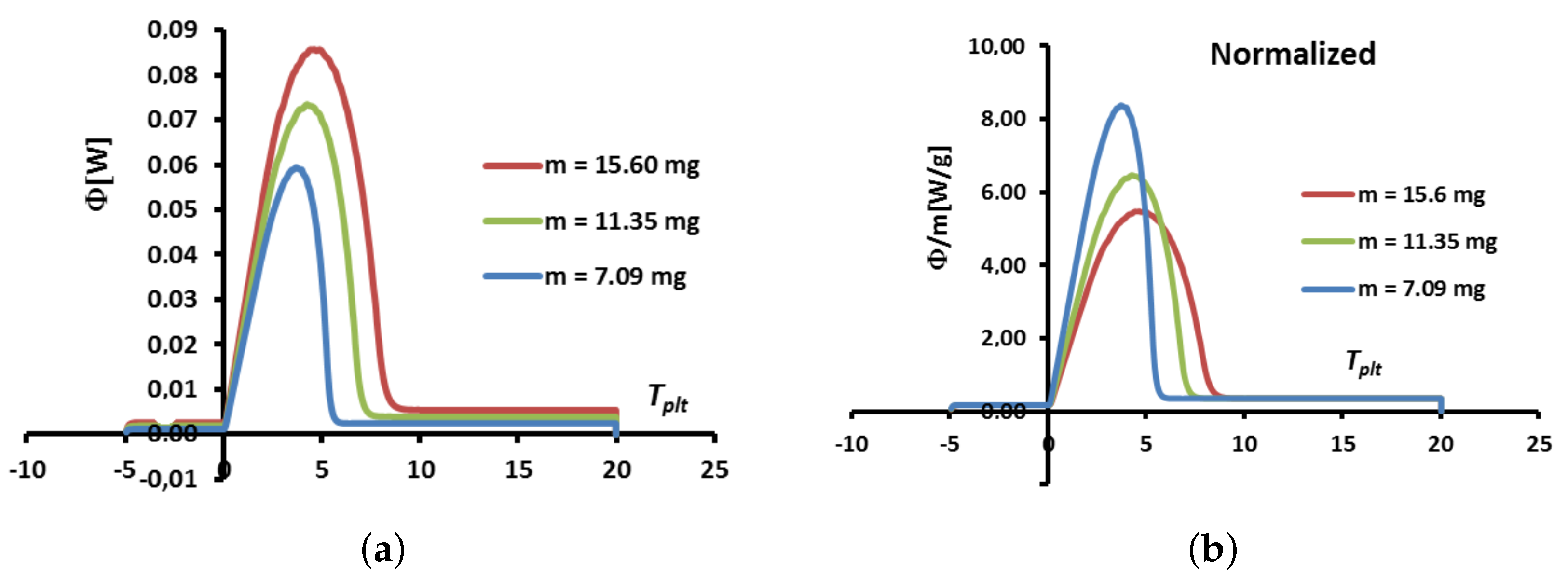
4.1.4. Influence of the Mass of the Sample
The idea here is to vary the mass of the sample, for a given heating rate fixed at
. In
Figure 10 are depicted the corresponding thermograms in function of the plate’s temperature. Two representations are used: the direct one in
Figure 10a and another one (the normalized curve), in
Figure 10b, where the heat flow-rate
is divided by the mass of the sample.
The usual observations are that the higher the mass, the larger the width is and the larger the maximum heat flow-rate
are. Moreover, as seen in
Figure 10b, the normalized curves, obtained by dividing by the mass, are still different. However, in each case, the corresponding specific enthalpy is unique (from the thermodynamic principles) so it is illusory to use the shapes of the curves to determine the specific enthalpy.
4.1.5. Practical Consequences.
We have indicated in
Figure 4 that, apart from the temperature range of the phase change, in the sensible zone, it is possible to determine the specific heat capacity by the formula:
deduced from the models with homogeneous samples [
1,
2,
3,
4,
6]. However, we can observe that the temperature inside the sample
is almost uniform, the temperature differences being of the order of a few tenth of K.
So, in this sensible zone, the specific enthalpy
h is given by integration of this value of
c (corrected to obtain the true temperature
by the relation (
10)). By extension certain authors define an artificial heat capacity, called equivalent capacity
, with a similar formula as Equation (
8) but
even during the phase transform.
Moreover, the calculation of an “apparent” enthalpy
is proposed by an integration of
versus
and considering this plate’s temperature as “the” temperature of the sample [
1,
2,
3].
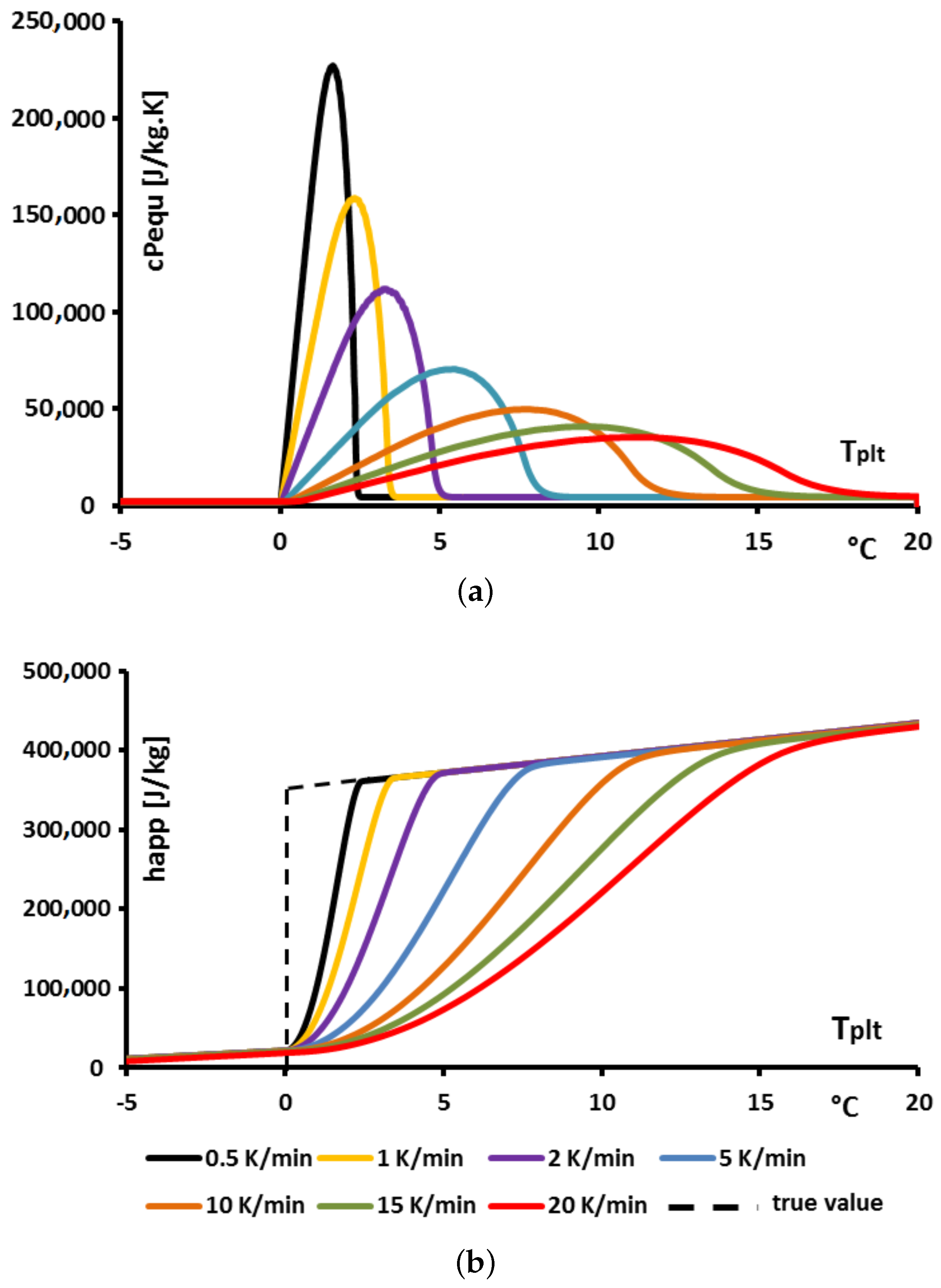
Given the preceding analysis and the corresponding conclusions, it is noteworthy to mention that this equivalent heat capacity representation, based on the integration of the heat flow-rate with respect to the plate’s temperature, lead to a completely incorrect determination of the enthalpy function, for example even if we consider a supposed melting temperature range.
Thus, in the present case of pure substances, such a definition leads to various functions for this equivalent heat capacity
, as depicted in
Figure 11a and for the apparent enthalpy
in
Figure 11b where different heating rates are considered.
Firstly, it appears clearly (as it could have been inferred from the previous results) that the obtained functions
are not independent from the operational conditions i.e., in the present case, dependent on the heating rate. Yet, the enthalpy being a function of state, it cannot be dependent on the heating rates. In the present case of pure substances, it is known that this function is an Heaviside one. In other words, any method implying a dependency of the enthalpy function with the heating rate is totally inconsistent with the laws of thermodynamics. Moreover, we have shown [
9,
10] that this method which enlarges the temperature range of melting is not representative of the true energy storage kinetics, the PCM seeming less efficient.
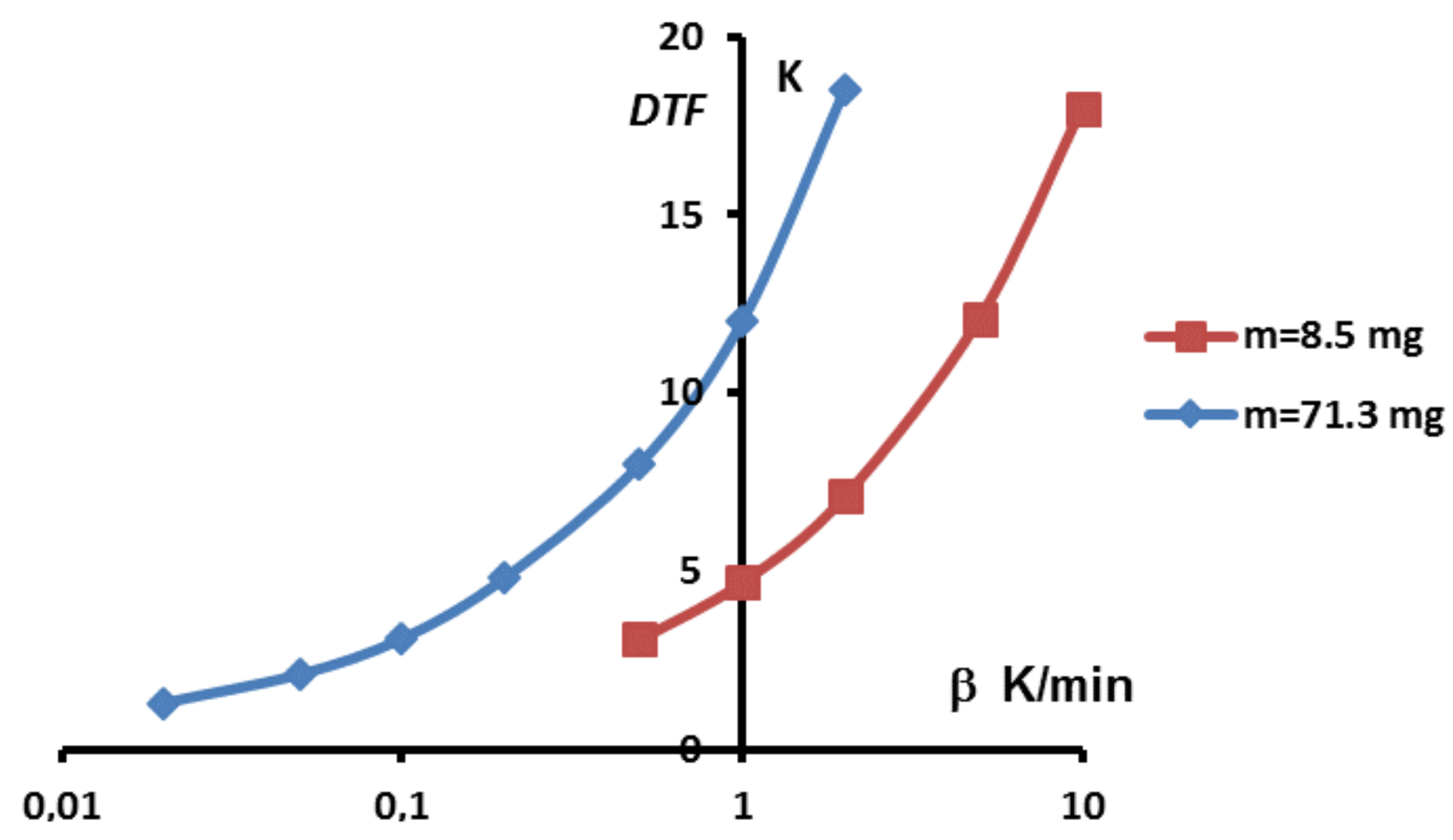
Secondly, one can see that the dome zone of the equivalent heat capacity is narrower for lower values of the heating rate or the mass. However, the above results have shown that temperature gradients were still present even with low heating rates. Given that the true solution is a Dirac function, it is tempting to consider theses curves as different approximations of this Dirac function, having a result that should converge towards the correct value for infinitely low heating rate. Unfortunately, such an approach is still imprecise. Indeed, when trying to further decrease the heating rate, one usually faces two drawbacks: (i) the ratio signal to noise is lowering and uncertainties consequently grow; (ii) generally, to maintain this ratio signal to noise to an acceptable value lowering the heating rate requires to use larger samples, that is to say to increase the mass, which leads to an increase of the width as shown before. This last point is further developed in
Figure 12 where is shown the width of the peak, i.e., the difference between the foot and melting temperatures,
, in function of the heating rates for two different masses.
One can note that there always exists a certain width of the peak. Moreover, depending on the mass sample, the obtained width, is not better for a lower value if the mass is too high. Thus, in the case of sample, a width is obtained for , and a similar arises with for a sample. In other words, there is primarily no boon when decreasing experimentally the heating rate if this requires to increase the mass.
4.1.6. Melting Temperature and Specific Latent Enthalpy
Melting temperature
We have particularly noticed that the temperature field of the sample is very different from the temperature of the plate
and non uniform, when the melting occurs. However, before the melting (before the time of the peak of the thermogram) or when this melting is finished (largely after the time of the peak), we have already mentionned that the temperature inside the sample is almost uniform. However, if this temperature is homogeneouly, its value ,
is different from the plate temperature
because the thermal resistance
R (such as
) between the sample and the metallic cell. We can use, to determine
, the ancient model of homogeneous sample [
4] which gives (solid phase):
So, if we consider that the melting begins (left foot of the peak) when
, i.e., at a time
where
, we observe that apparently the temperature
depends on the heating rate.
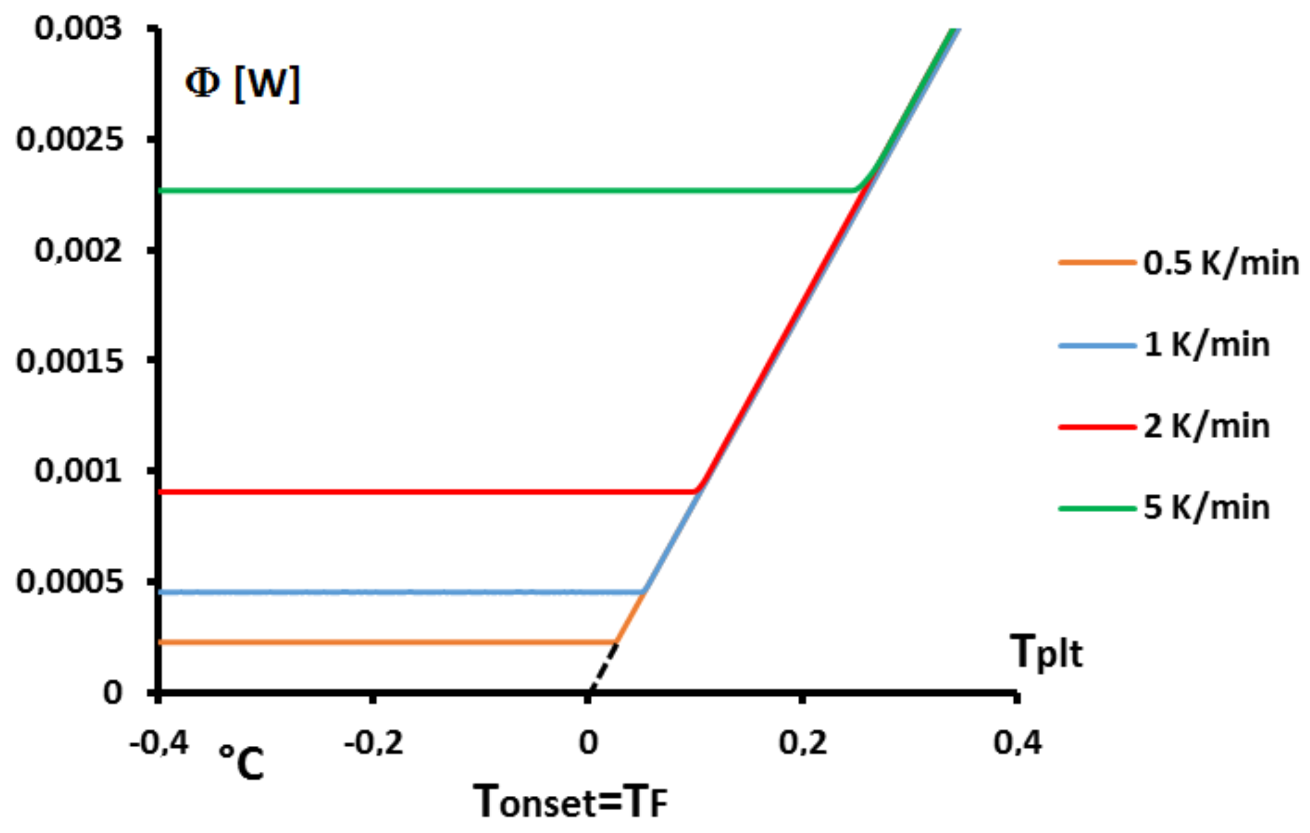
Figure 13 represents an enlargement of
Figure 9a around
where we observe that the curves of the beginning of the left part of the peak are aligned straight lines and intercept the zero line (where
) at
. This can be perfectly explained by the model with homogeneous sample, but the model we present gives the same results at the beginning of the melting when the solid is at
and the quantity of liquid very small.
In fact, to determine
it suffices to extrapolate the line having the greatest slope of the left side of the peak for only one experiment for a given heating rate
. If it seems that this construction is similar to the construction of the line giving the
presented in
Figure 8, there is a difference because we take into account the intersection with the zero line (
) and not the interception with the line joining the sensible lines as in
Figure 8.
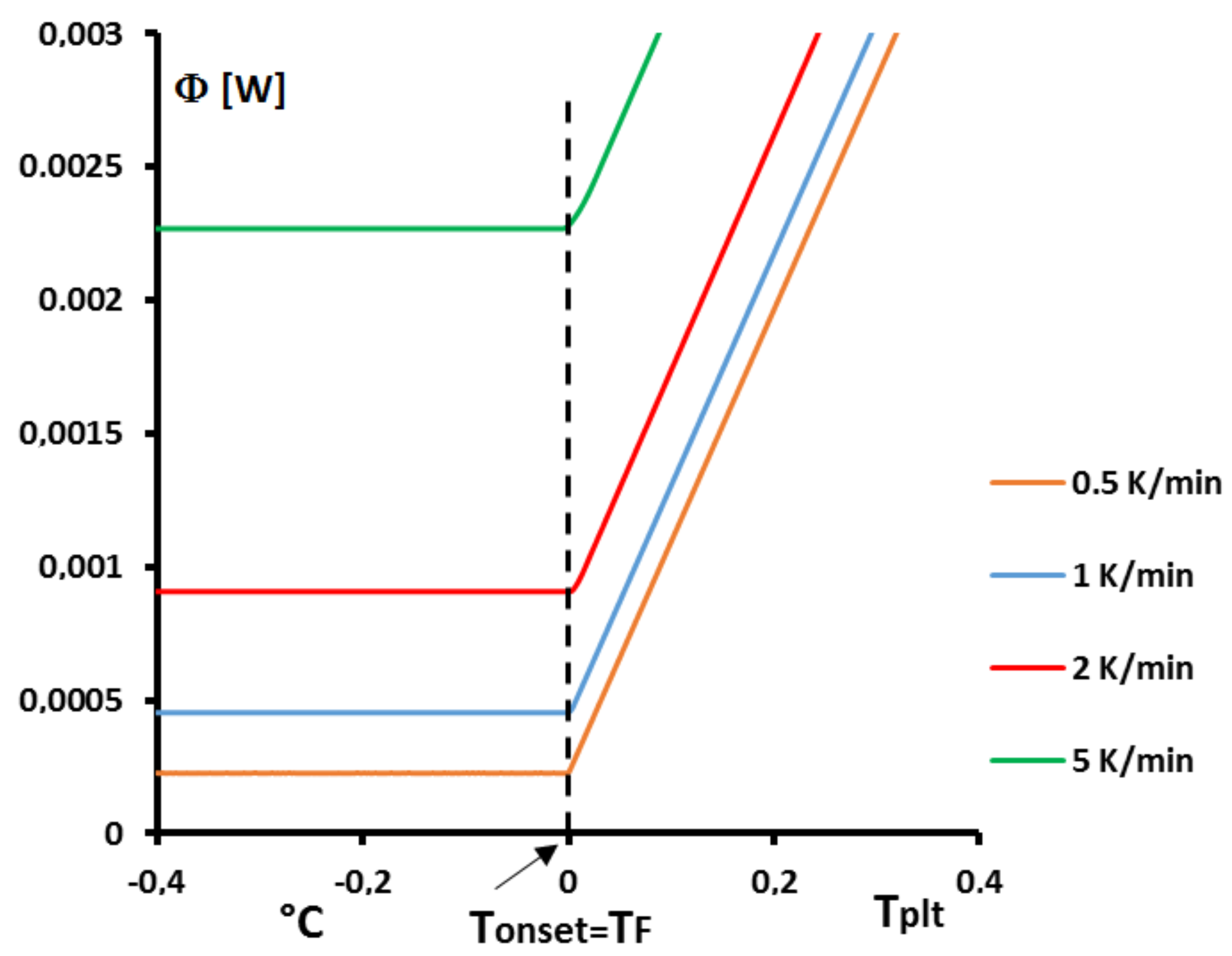
We must recall that, if we use for all calculations at all heating rates
, the variation of the temperature of the plate by the function:
it corresponds to a particular calibration in temperature of the calorimeter where the temperatures are located to the zero line. In fact, the calibration in temperature is made by experiments with pure substances as described herein. If, these experiments of calibration (theorically, one experiment at one heating rate is necessary) for different pure substances were made with this extrapolation to the zero line , the zero line is calibrated in temperature.
If the calibration is made, more traditionally, at each heating rate, using
, but with
defined as in
Figure 8, we must make the correction in conformity with Equation (
10) and the thermograms in a
scale are shifted as we can see in
Figure 14.
Latent Heat
The determination of the latent is classically presented as the measure of “the peak area”. It is absolutly correct, for the pure substances when the heat capacities of the liquid and the solid are equal. So, this area is delimitated by the thermogram and a horizontal straight line joining the sensible lines before and after the peak. This can be explained either with the homogeneous model or with our heterogeneous model [
1,
11].
However, our model permits to give the true delimitation of the peak to determine the latent heat of melting even in case where the specific heats of solid and liquid are different. We can demonstrate [
11] that the latent heat of melting is given by the equation:
where:
the integration for each instant is for
the entire volume of the sample.
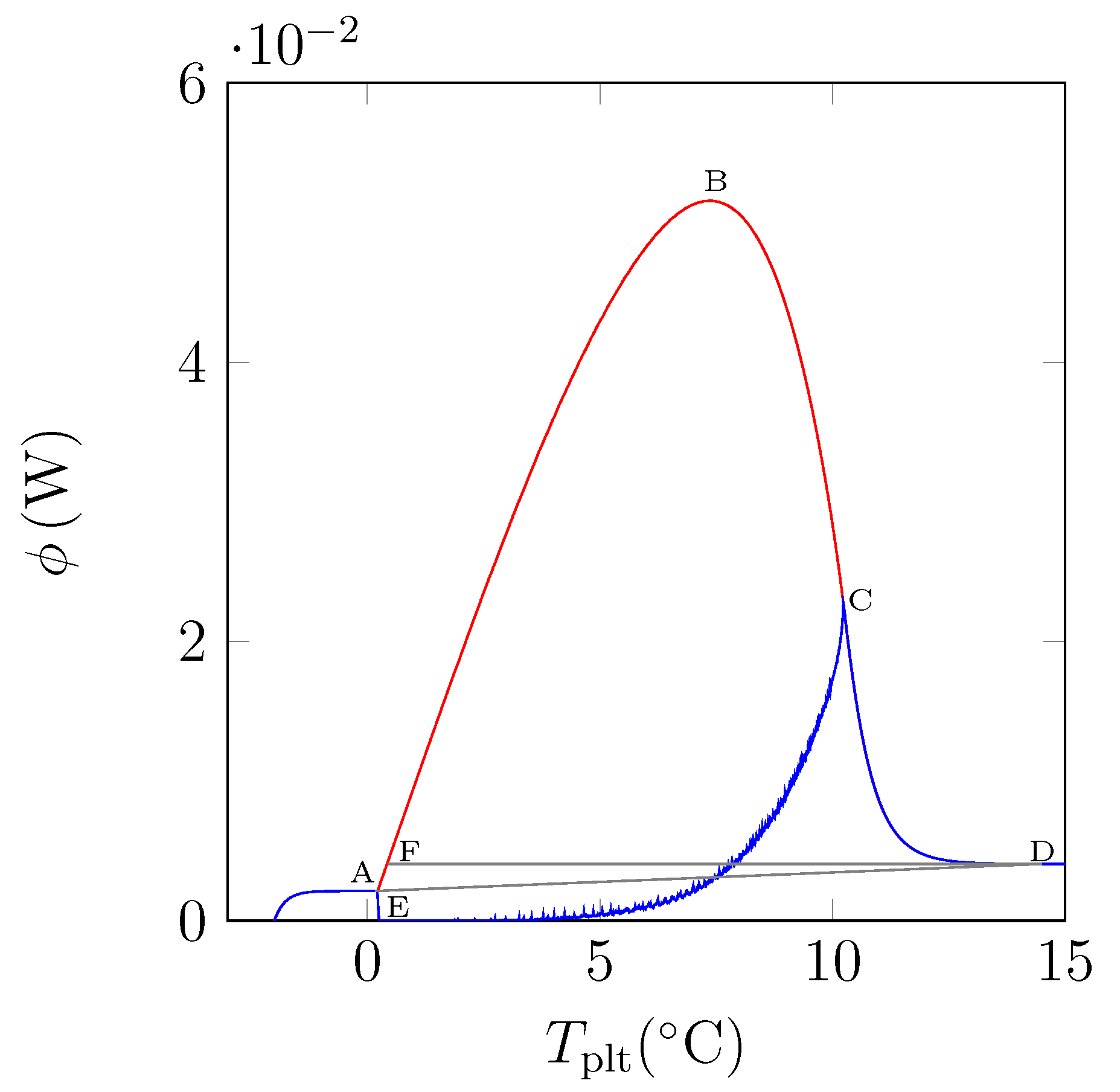
In
Figure 15, we have plotted a thermogram for the melting of ice at 5 K/min (in red) and the function
(in blue). The specific latent heat of melting
is given by the area delimitated by the closed curve AECBFA of
Figure 15 divided by
and the mass of the sample.
We can notice the confirmation that the location of the point C at indicates the instant of the desappearance of the last solid particule is the inflexion point of the right side of the peak. We also confirm that the curve CD represents the return to equilibrium, the sample having a distribution of the temperature from at the center with the last particle to the programmed temperature of the periphery. At the instant of point D, as already indicated, the sample is completely liquid at an almost homogeneous temperature.
In fact, the curve
is difficult to plot, because it is necessary to know the temperature and mass fraction fields which is only really possible with the model and not experimentally. However, this study permits to evaluate the traditionnal determination either by the area ABD recommended by the calorimetrists or the area FBD in conformity with the model considering the sample as homogeneous [
6,
12]. We have found for water (whose liquid or solid specific heats are very different) discrepancies ≤1%.
4.1.7. On the So-Called “hysteresis Phenomenon”
During melting, it has been shown that the spreading of the DSC curve does not mean that phase transition occurs on a temperature range above , and indeed, for pure substances, this phase change takes place at a constant temperature. Similarly, and if one assumes there is no supercooling, a spread DSC curve under cooling will not imply that solidification is occurring on a temperature range.
So, in contrast to what is often encountered, it is wrong to describe the phase transition by two characteristic temperature ranges obtained respectively from DSC curves in heating and cooling modes. In other words, there does not exist such hysteresis phenomenon.
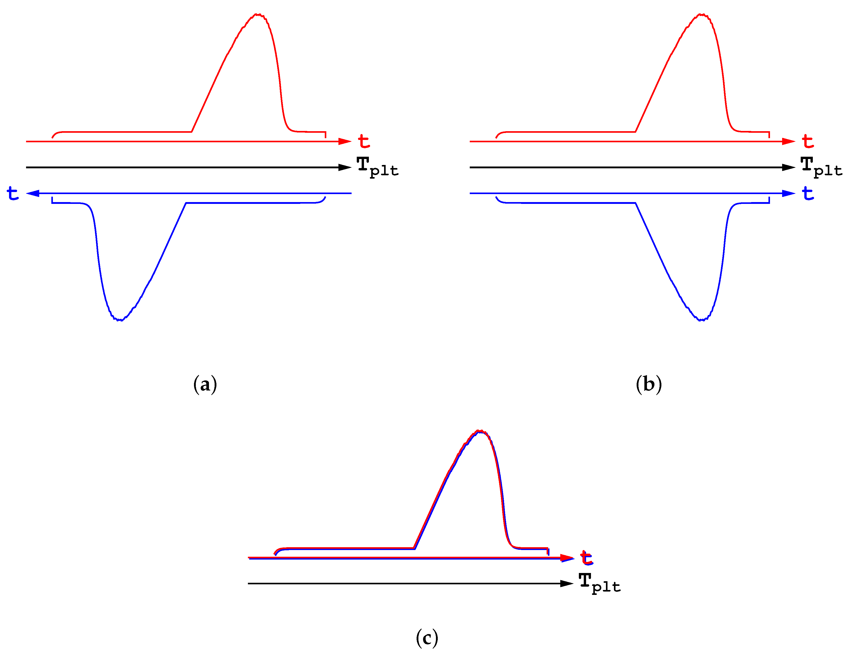
Let us further highlight this statement and show how and why such a misunderstanding is encountered. Thus, in
Figure 16a are represented two DSC curves in heating and cooling modes, with the same rate for both the heating and cooling parts. In
Figure 16a are presented the corresponding thermograms, showing the heat flow-rate in function of the temperature of the plate
. One can see the usual spreading of the DSC curves, towards the right and the left respectively, as explained before. However, such a representation is an artefact obtained since the plate’s temperature varies linearly with time. On this
Figure 16a we have added the time scales which can be considered in an opposite direction. If we restablish the direction of the time scale for the cooling curve, we obtain
Figure 16b. And finally, by taking the absolute values, both the endothermic and exothermic transformations can be drawn with the same scale in
Figure 16c. One can see that both DSC curves are superimposed, which proves that there is no fundamental differences between the melting and the solidification. Consequently, it is clear that no hysteresis phenomenon exist at all.
4.2. Aqueous Saline Solutions
4.2.1. Presentation
Given the previous analysis and practical remarks on the interpretation of DSC curves, it is now proposed to extend the purpose to binary mixtures that undergo their phase transition on a temperature range and not at a fixed temperature anymore. The first example we present concerns the case of saline solutions which is particular because the solid phases are pure. In this section, we treat the case where the solid phase is the ice, the cases where the solid phases would be the salt will lead to similar conclusions.
The initial mass concentration of the solute (salt)
is defined by:
being the initial mass of the solute and
being the initial mass of the solvent (water).
In the goal to present general results independent of the nature of the solute, we will give same results considering the molar concentrations (for the ionic solutes it will be, in fact, osmolar concentrations) defined as:
being the initial number of moles of the solute and
being the initial number of moles of the solvent (water).
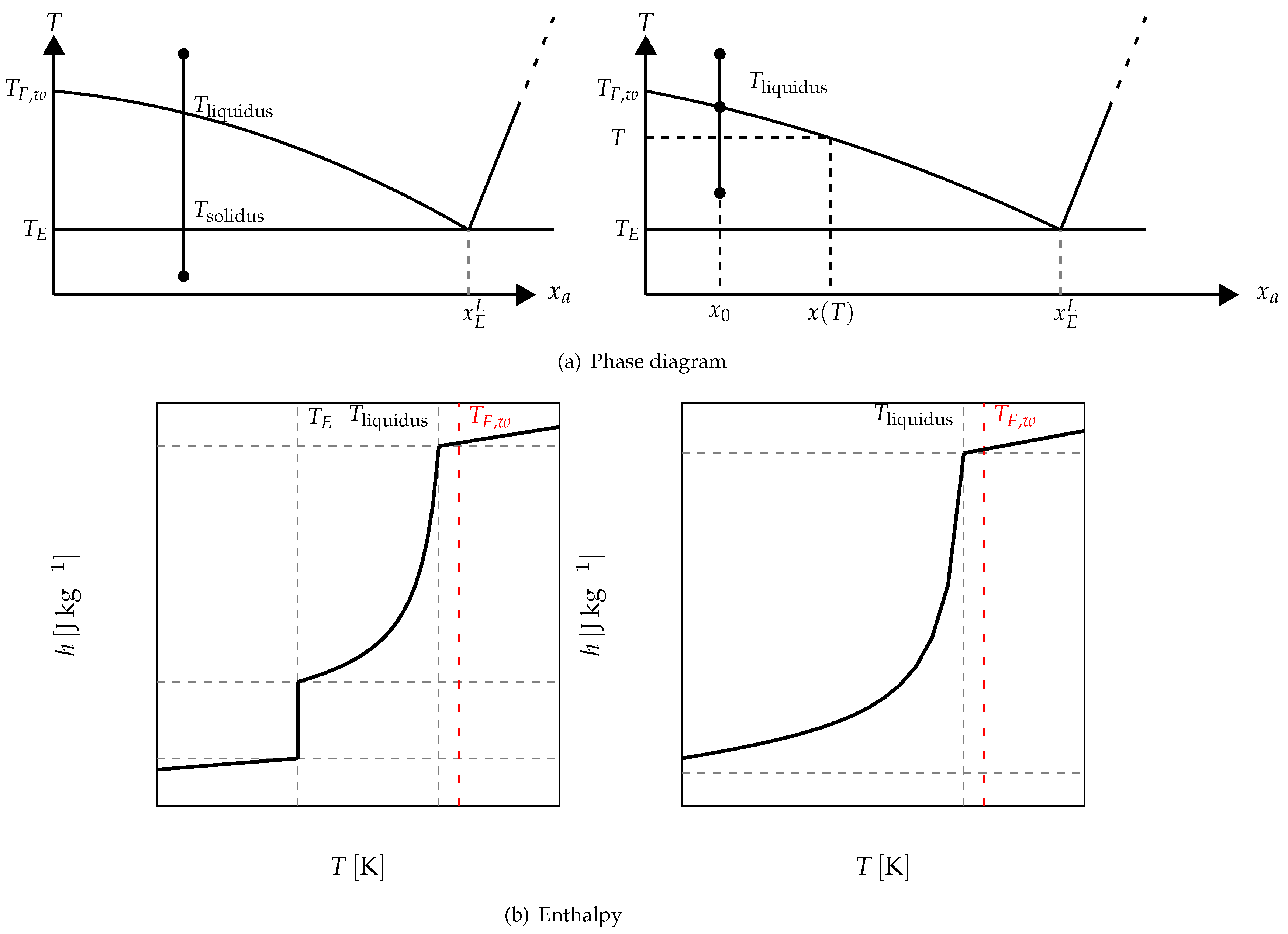
For example, in
Figure 17 it is schematized the phase diagram of a binary solution presenting an eutectic equilibrium. We also present, in this figure, two cases of the enthalpy following the investigated temperature range. When the melting begins at a temperature lower than the eutectic temperature
, we have the function depicted in the left. The value of the enthalpy when the melting begins at a temperature higher than the eutectic temperature is given on the right.
Above the eutectic temperature
, the enthalpy corresponds to a progressive melting (equilibrium, at
T, between the pure ice and the solution whose mass concentration
is given by the phase diagram (see
Figure 17)). This progressive melting ends at
which is the temperature of the equibrium of pure ice and the solution at the initial mass concentration
.
The phase diagram permits to determine the mass fraction of liquid water at the local temperature
T (see
Figure 17) defined as:
by the equation:
and
.
For the sake of clarity, in this section:
From a practical point of view, this does not alter the generality of the conclusions but only simplify the calculations and the analysis, the number of meaningful parameters being reduced.
With these assumptions, the enthalpy function is:
n.b.: the reference state has been chosen at
.
Thus, the specific enthalpy is dependent on the temperature and the initial mass concentration (via
) as is shown in
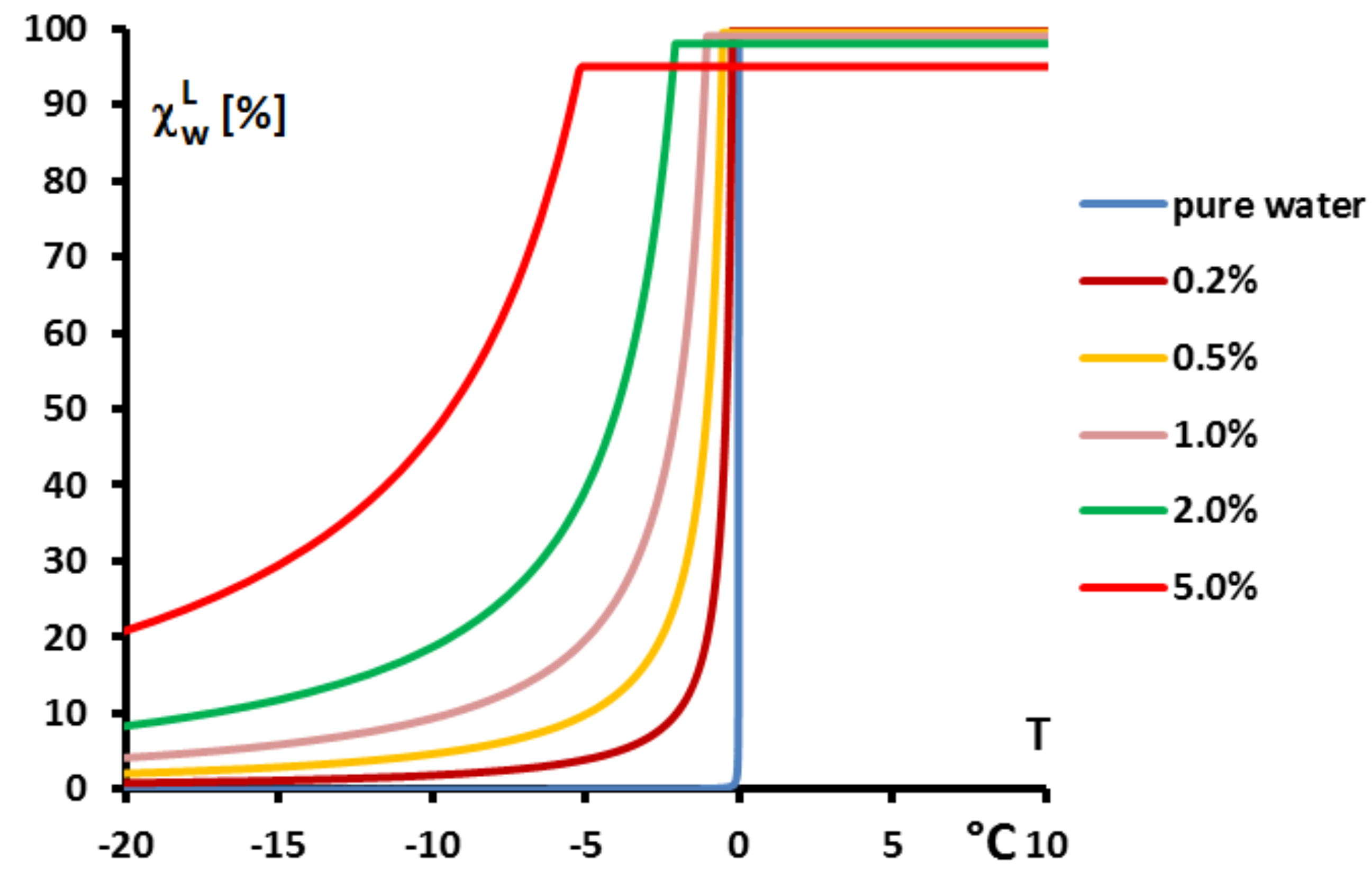
Figure 18.
Figure 19, giving
, confirms that the two-phase equilibrium spreads on a temperature range depending on
(progressive melting). In other later figures we also present the temperature range of melting by the function
versus
T.
For these cases of enthalpies, we have presented several papers [
13,
14] describing the construction of the thermogramms for such solutions. The model is the same that the one presented for the pure substances, but with a function
h different given, in our simplified case, by Equation (
18). As indicated above (
Figure 19) this function depends on the temperature and, via the temperature
, on the initial mass concentration.
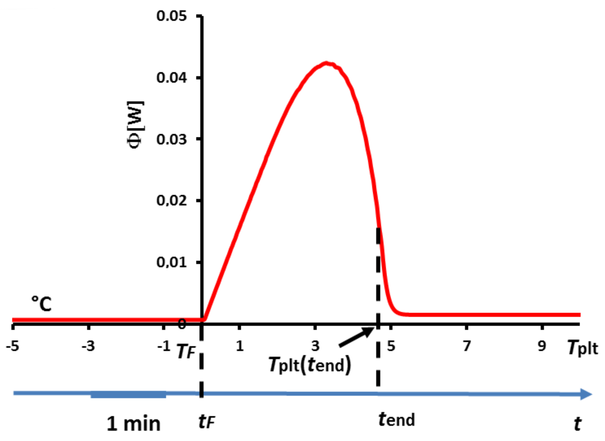
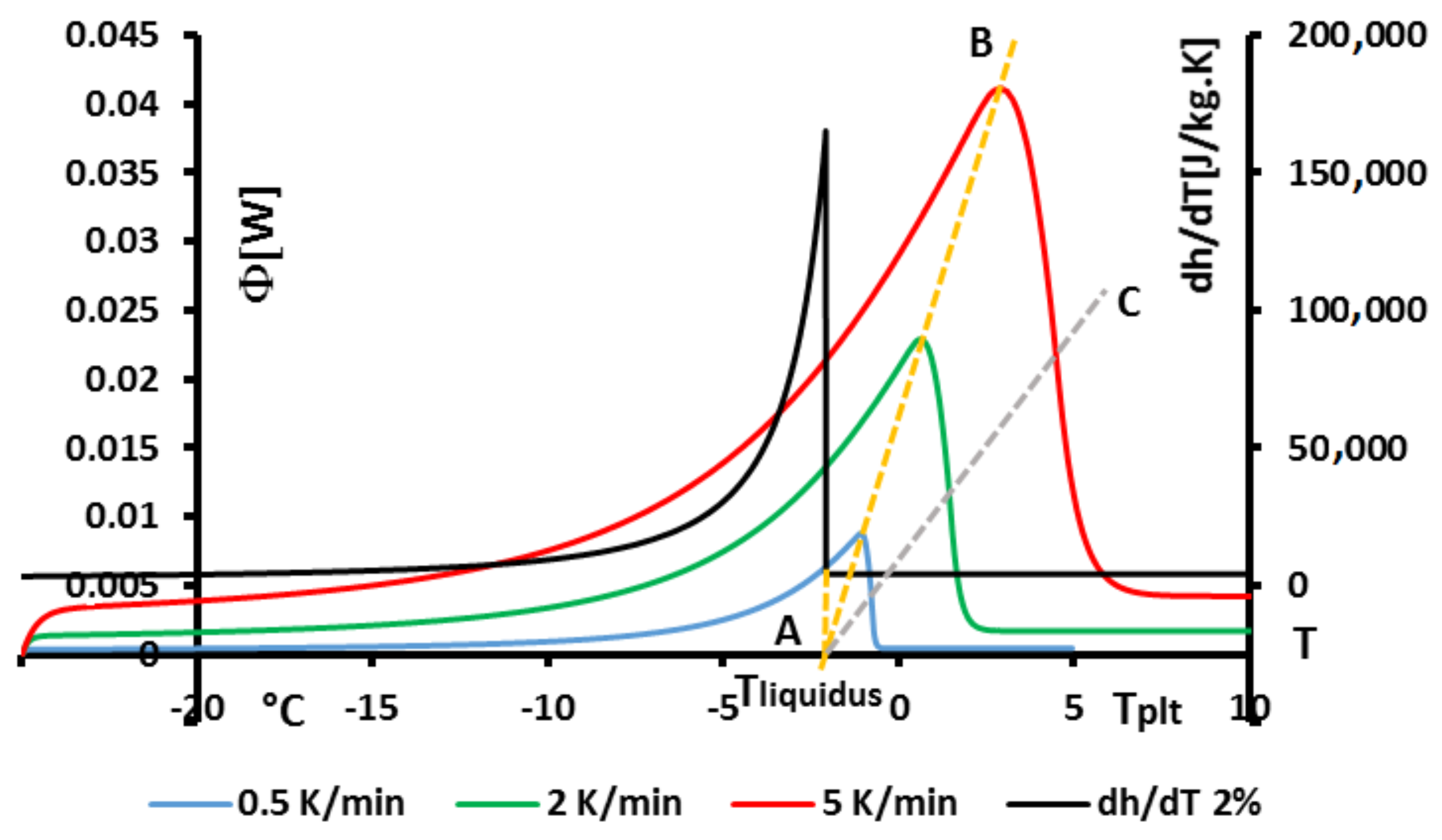
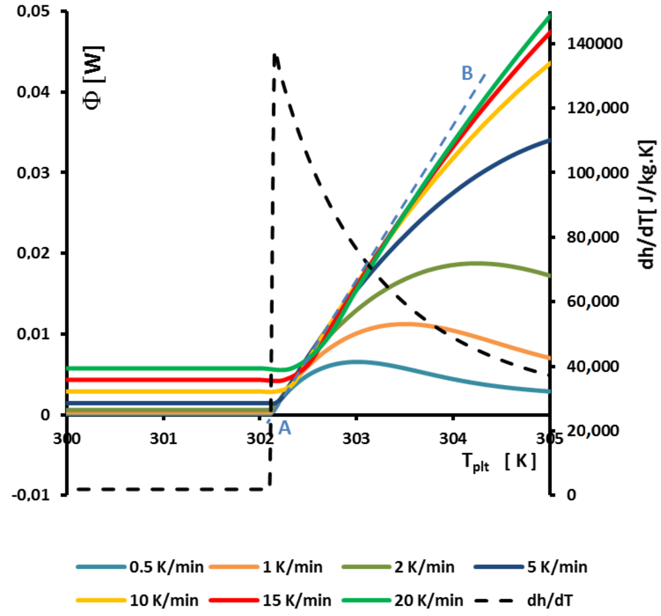
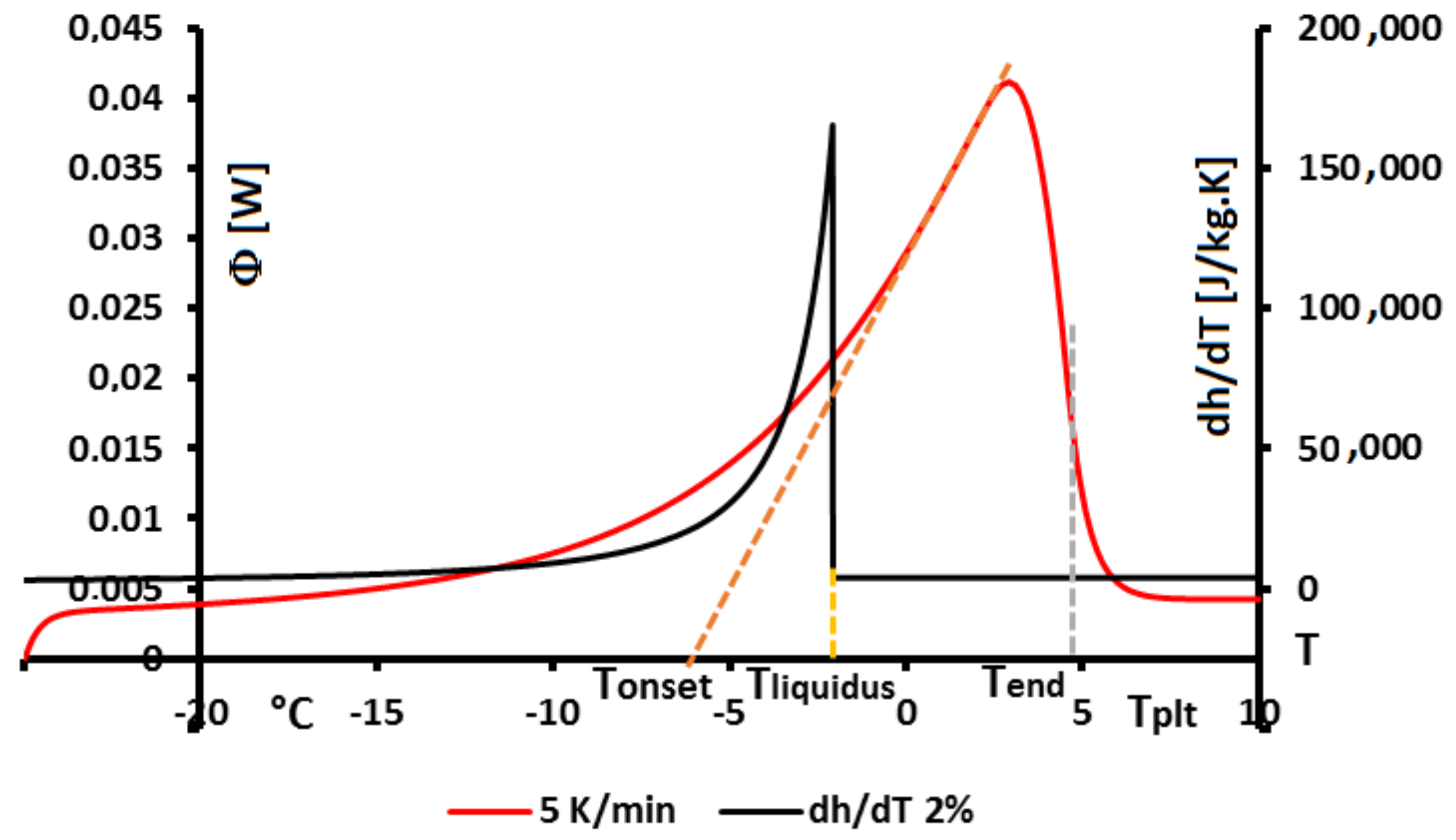
In
Figure 20 we present, as an example, the case of the thermogram for the melting at 2 K/min of an aqueous solution with
= 2%. This thermogram is formaly compare to
the derivative of the corresponding curve of
h given in
Figure 18 and which also represent thermodynamically the spreading of the melting up to
= −2.07
(confirmed in
Figure 19). In this
Figure 20 we recall that the abscissa line represents the programmed temperature of the calorimeter’s plate (time in fact) and the local temperature
T for
.
We mainly observe that the thermogram does not represent the real phase change at a first glance. As for the pure substance, the thermogram presents a peak at an apparent temperature (
) range higher than the temperature of the end of melting, i.e.,
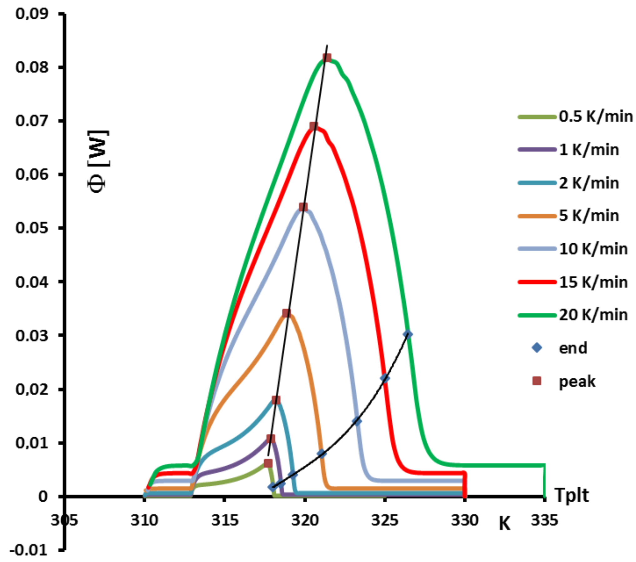
. Obviously, by analogy with the pure substances, this enlarged shape of the peak is due to the conduction heat tranfers inside the sample. This is, for example, confirmed by the next
Figure 21 where we present thermograms at different heating rates
. We have also demonstrated that the last particule of solid disappears, as for the pure substances, at the instant
corresponding to the inflexion point of the right part of the peak (
in the
scale).
In
Figure 20 we have also plotted the classical straight line to determine the
, but with the method described above for the pure substance, where
is determined at the intersection with the zero line (to be in conformity with our calibration). We see that this value of
has no significance and is not linked to any thermodynamical characteristic of the solution, particularly the temperature
. The temperatures
and
, defined as in
Figure 2, also have no significance.
The determination of this temperature
is given by the method of extrapolation at the zero heating rate (
) [
15]. It consists to join the tops of the peaks of thermograms at different heating rates (see
Figure 21). For aqueous solutions the obtained line (AB) is a straight line which can be extrapolated to the zero line giving obviously
(an imaginary flow rate at
= 0 would be identical to
). We can also use the straight line (AC) which joins the inflexion points on the right part of the peak, but this line is less easy to plot.
Remark 1. we emphasized in Section 4.1.5 to specify that it was useless and impossible to program low heating rates especially if it forced to increase the sample mass. However, here the extrapolation to is not experimental but mathematical. It is not necessary, as indicated in Figure 21, to experiment with extreme low heating rates. 4.2.2. On the So-Called “Hysteresis Phenomenon”
h or
are thermodynamical functions characterizing the solution. For a solution, either on heating or on cooling (without supercooling), the same function
h as Equation (
18) must be used in the model. So, locally, it does not exist a hysteresis. However, concretely, the function
being not symmetrical, this means that the heating and cooling thermograms have different intrinsic shapes as indicated in
Figure 22. They represent the same phase change. At no moment, any hysteresis phenomenon must be assumed to obtain such thermograms, even they have a non-symmetrical shape.
4.3. Case of Small Concentrations
4.3.1. Presentation
As a rule of thumb, it is very difficult to find very pure materials. For instance the PCM based on alkanes are solutions whose the highest purity is commonly between 98% and 99.5%. In addition, in cases where PCMs are dispersed there may be some slight dissolution in the PCM of the dispersant or microencapsulation products. This section is focused on the small solute concentrations. The main results of the preceding section on saline solutions can be applicable, but consequences adapted to these small solute concentrations will be highlighted.
Generally the total amount of impurities is given in mass. However, the nature and quantities of each impurities (solutes) should be known because it is the sum of the molar fractions (of osmolar fractions in case of ionisation of the solutes in water) which is needed to calculate the cryoscopic lowering.
The cryoscopic lowering is the difference between the melting temperature of the pure substance
and the equilibrium temperature
at the molar concentration
where the
are molar fractions (or osmolar fractions) of each impurity
i. For the very low concentrations, the cryoscopic lowering is given by the Raoult’s law:
with
the ideal gas constant and
the molar mass (in kg) of the solvent (water).
In such a case, where the amount of impurities is only of the order of a few percents, there are already important modifications of the shapes of the thermograms which are now going to be analyzed and the consequences on the phase changes evaluated.
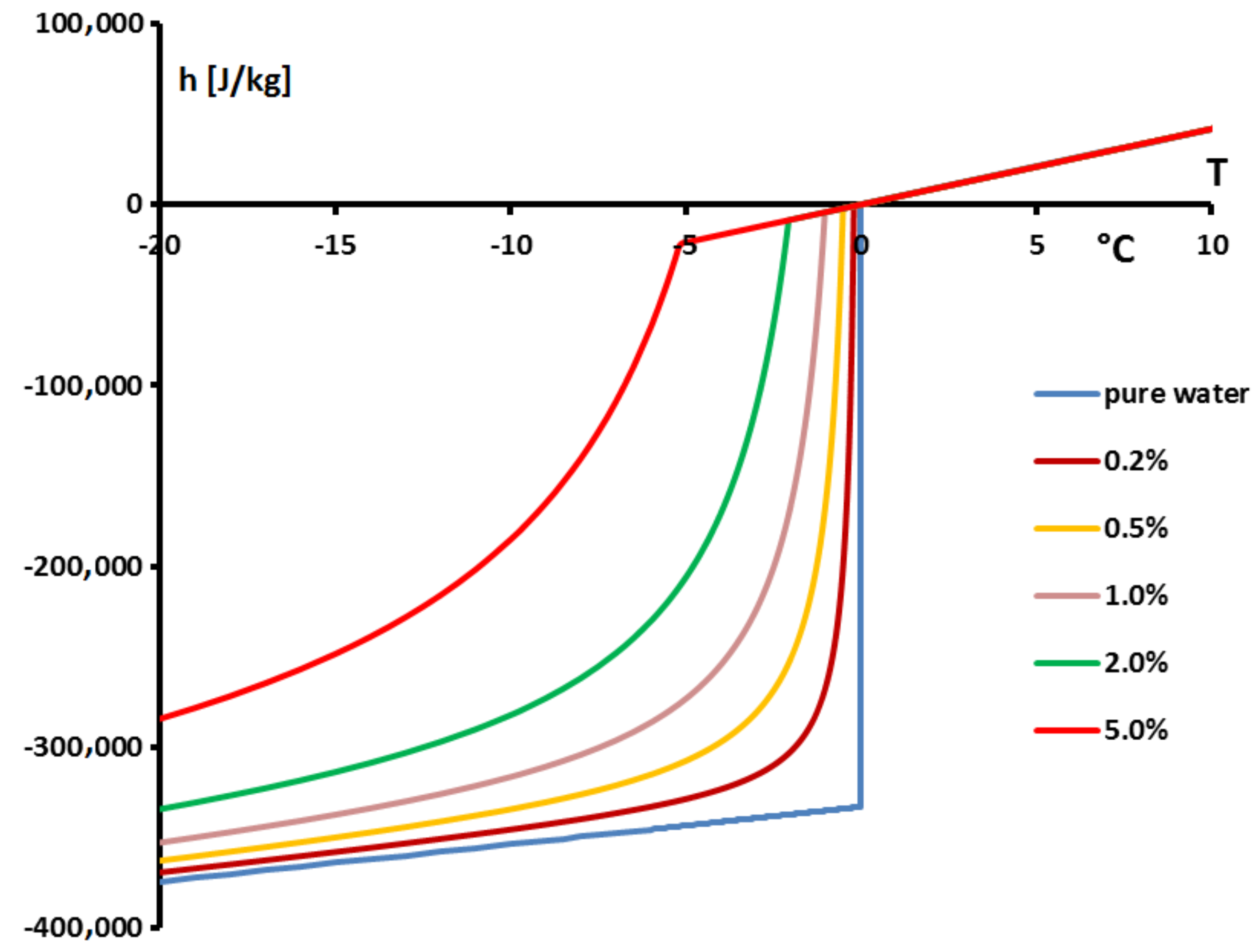
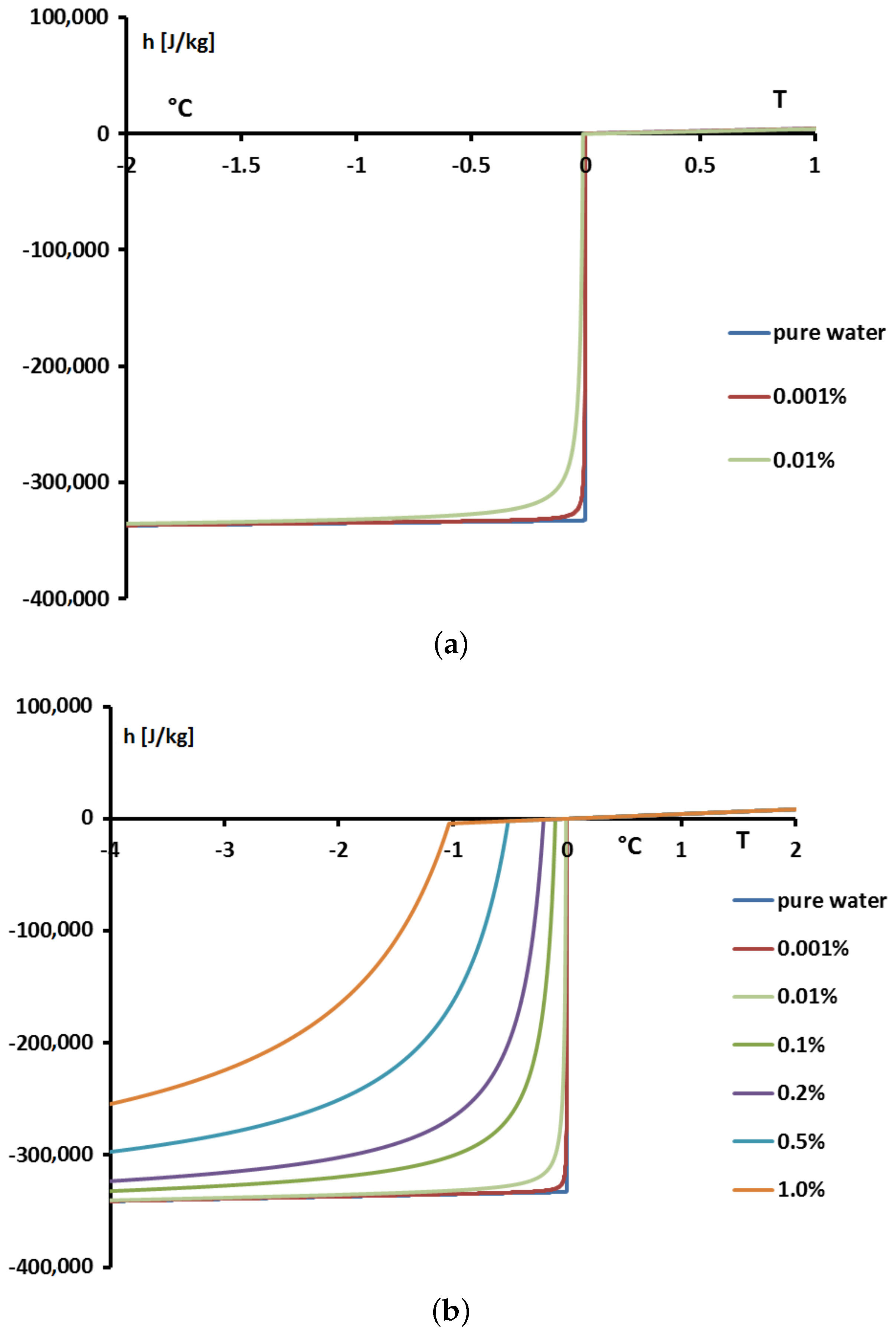
In
Figure 23 we present, for solutions with
, the values of the enthalpies
h calculated from Equation (
18) with
calculated from the Raoult’law Equation (
19). To anticipate the results presented below, we made the difference between the concentrations extremely low (
= 0.001% or 0.01%) in
Figure 23a and the others (
) in
Figure 23b.
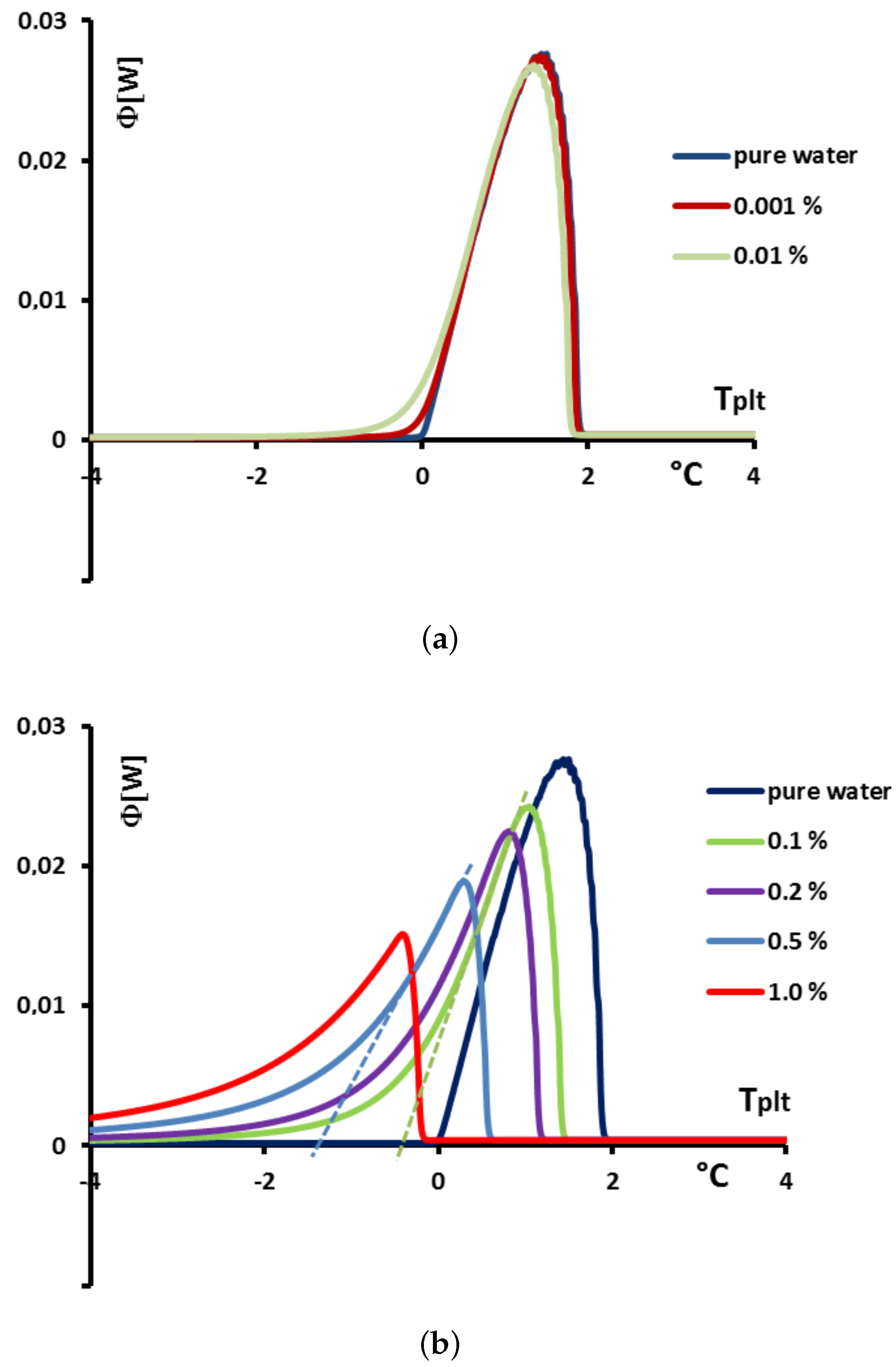
Applying our model with the value of
h calculated for
Figure 23, we present in
Figure 24 the thermograms calculated for melting at 0.5 K/min.
In
Figure 24a, we present the thermograms of pure water and the thermograms for very dilute solution (
= 0.001% and 0.01%). For the melting of pure ice in the presence of these solutions of extreme purity, the thermograms have a shape useable for pure water except the rounded corner of the left foot of the peak. However, this figure, despite this deformation gives the same
that for the pure substance.
However, in the second
Figure 24b the concentration
are sufficiently high to involve important modifications of the shapes of the thermograms. In this case, as it has been presented in
Figure 20, the
classically determined has no significance and is different from the desired temperature
. However, taking into account the smallness of the concentrations, the difference
is relatively small, of the order of the accuracy due to the calibration. For example, for a concentration of
= 0.1%, this difference is 0.2 K and for a concentration of
= 0.5% this difference is 0.9 K, the differences with the temperature of melting of the pure substance
being 0.3 K and 1.4 K respectively.
4.3.2. Discussion
It is possible that, in industrial applications, these uncertainties are accepted. However the error would be to consider the PCM as pure with a fixed melting temperature evaluated at
. The fact that these PCM are solutions has more important consequences as we can already guess with
Figure 19 clearly showing that the melting does not take place at fixed temperature but over a wide range of temperature.
To evaluate, with these small concentrations, this spreading of melting over the temperature, we present in
Table 1 for each concentration,
(calculated by Equation (
19)),
, the temperatures where the mass fraction of liquid (calculated by Equation (
17)) are
= 10%, 50% and 90% respectively and finally this mass fraction at the evaluated
.
The example of the small concentrations described in this section corresponds to PCM with good, even very good, purity. However,
Table 1 indicates that is not pertinent to consider this PCM as pure. For example, for
= 1%, for the
given by the PCM sellers or given by own experiments, about 45% are already melted at this temperature and the melting has begun about 10 K before this onset temperature. We are not sure that it corresponds to an optimized latent heat storage.
4.4. Solid Solutions
4.4.1. Presentation
This section concerns binary solutions where the two compounds are completely miscible into each other, in solid or in liquid phases, which lead again to a phase transition spread over a temperature range.
In a previous paper [
16], we have simplified the problem, presenting an ideal solution. The results presented here are issued with this assumption but the general commentaries could be relevant for any non-ideal solution.
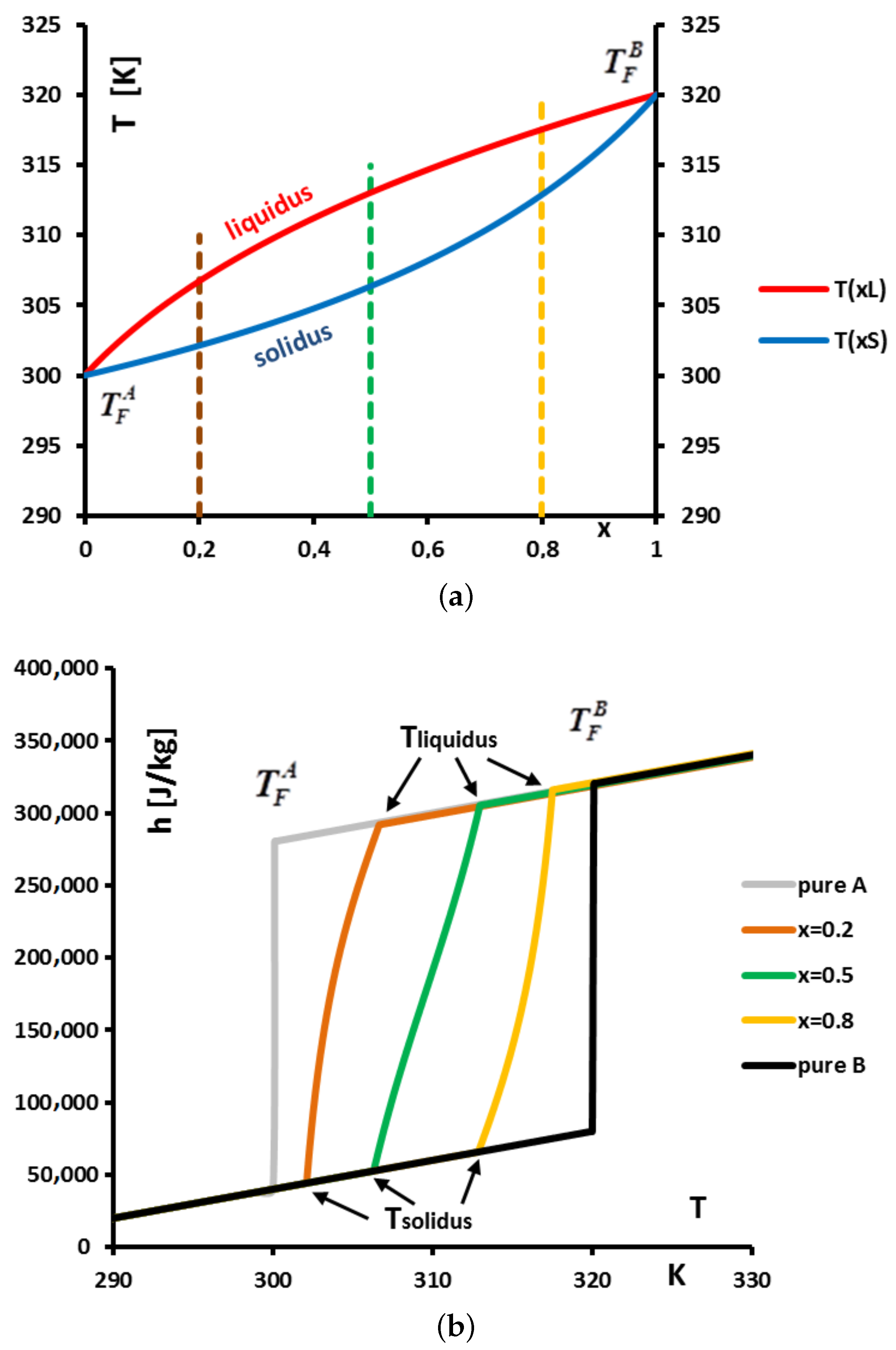
In
Figure 25a we present the phase diagram (at atmospheric pressure) for the ideal mixture of a substance
A (solvent) whose melting temperature when is pure is
= 300 K and a substance
B (solute) whose melting temperature when is pure is
= 320 K. We give results for three initial mass concentrations
= 0.2, 0.5 and 0.8. The initial mass concentration
is the initial mass fraction of the solute
B and if the initial mass of the two compounds are
and
, we have:
The phase diagram
Figure 25a presents two curves translating, for a given temperature
T, the equilibrium between a liquid solution at
and a solid solution at
: a
liquidus representing the temperatures
T versus
and a
solidus representing the temperatures
T versus
.
For these ideal solutions, we have established [
16] that the variation of the enthalpy, during the heating of a crystallized solution at
is given by:
or
where
and
.
and
are the mass latent heats of melting for the constituents
A and
B respectively. We have also made the assumptions that
and
(
means pure substance). The mass fractions
and
are defined by:
and these values are calculated considering the conservation of masses [
16].
The function
is determined by numerical integration of Equations (
21) and (
22).
In
Figure 25b we present the functions
for the three chosen concentrations and
for the pure substances
A and
B.
4.4.2. Results
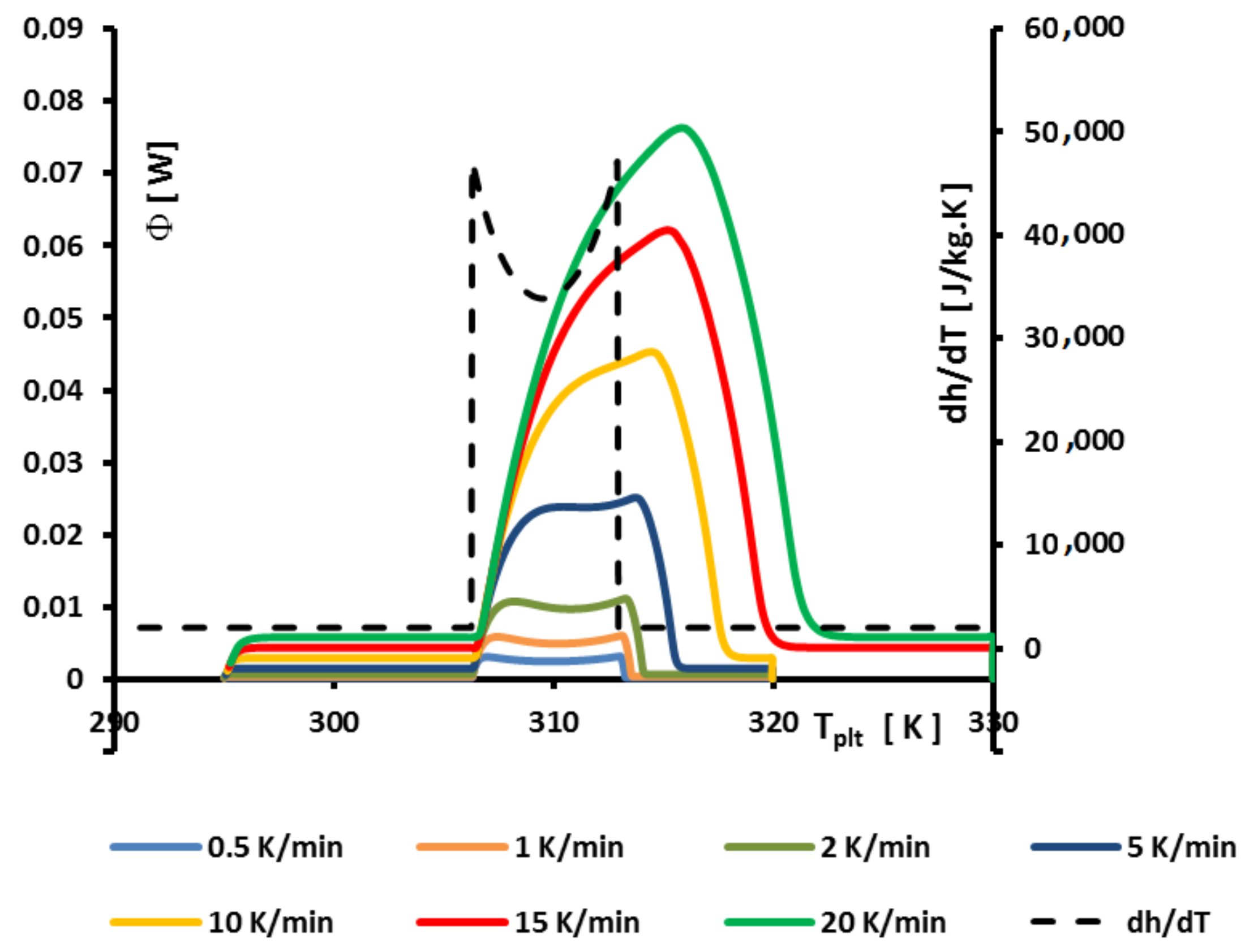
In
Figure 26,
Figure 27 and
Figure 28 we present the thermograms calculated with our model but with the
h functions calculated above from Equations (
21) and (
22). On these figures we have added the corresponding
deduced by a derivation of the curves of
Figure 25b and representing the actual phase transformation.
Remark 2. As for certain figures above, we recall that the abscissa line represents the programmed temperature of the calorimeter plate (time in fact) for the thermograms and the local temperature T for .
As for the pure substances and the saline solutions, we observe a strong difference between the thermogram and the thermodynamical properties represented by . The actual temperature range is not at all represented by the width of the thermogram which is wider. These thermograms are greatly enlarged towards the temperatures higher (or very higher) than . Except for the smallest , the shapes of the thermograms do not give information on the shape of the curve representing .
In the case of these solutions, the explanation of this discrepancy between the thermograms and the thermodynamical transformations they represent is due to the thermal transfers inside the cell. The melting and the corresponding concentration modifications (in conformity to the phase diagram) begin to the periphery of the cell and propagate towards the center, the last particule disappearing at a time corresponding to an inflexion point on the right side of the peak of the thermogram.
4.4.3. Determination of the Solidus
To determine
, we observe (see
Figure 25b,
Figure 26,
Figure 27 and
Figure 28) that at this temperature the value of
varie drastically as the pure substances. So, we can apply the method of the
as described in
Section 4.1.6 using the common tangent (AB) to the ascendant part of the peaks and an extrapolation to the zero line. We present such a determination, for
= 0.2, in
Figure 29. We find
= 301.2 K in conformity with the phase diagram of
Figure 25a.
Remark 3. Obviously this determination is correct if the substances A and B are perfectly pure. In case of a small concentration of impurities we can observe some rounded corners at the left foot of the peak. In this case, it is possible to find a method to determine a tangent useful to determine a as describe in Section 4.1.6. Indeed, to plot the solidus line of the phase diagram, experiments at different concentrations are needed.
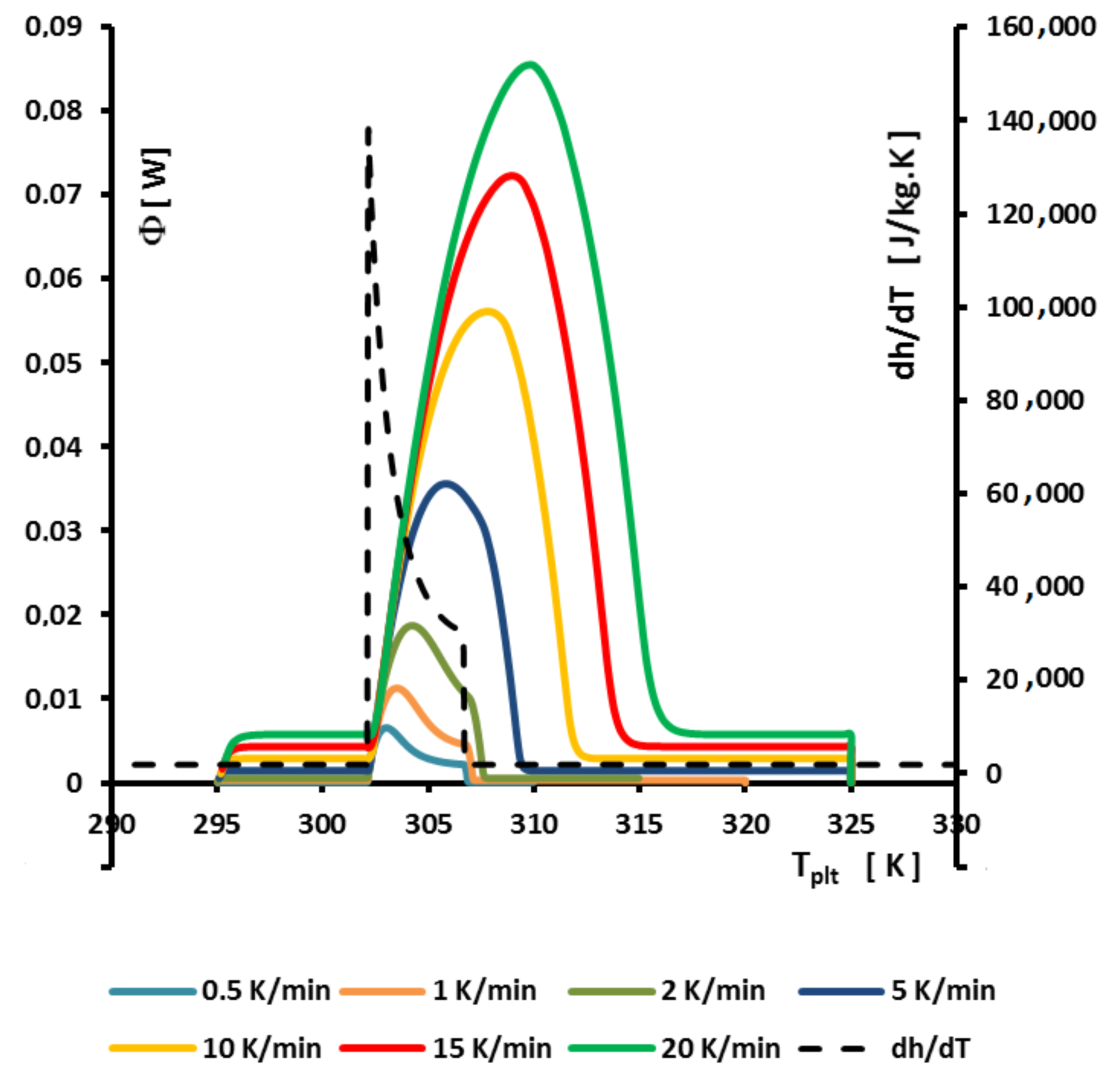
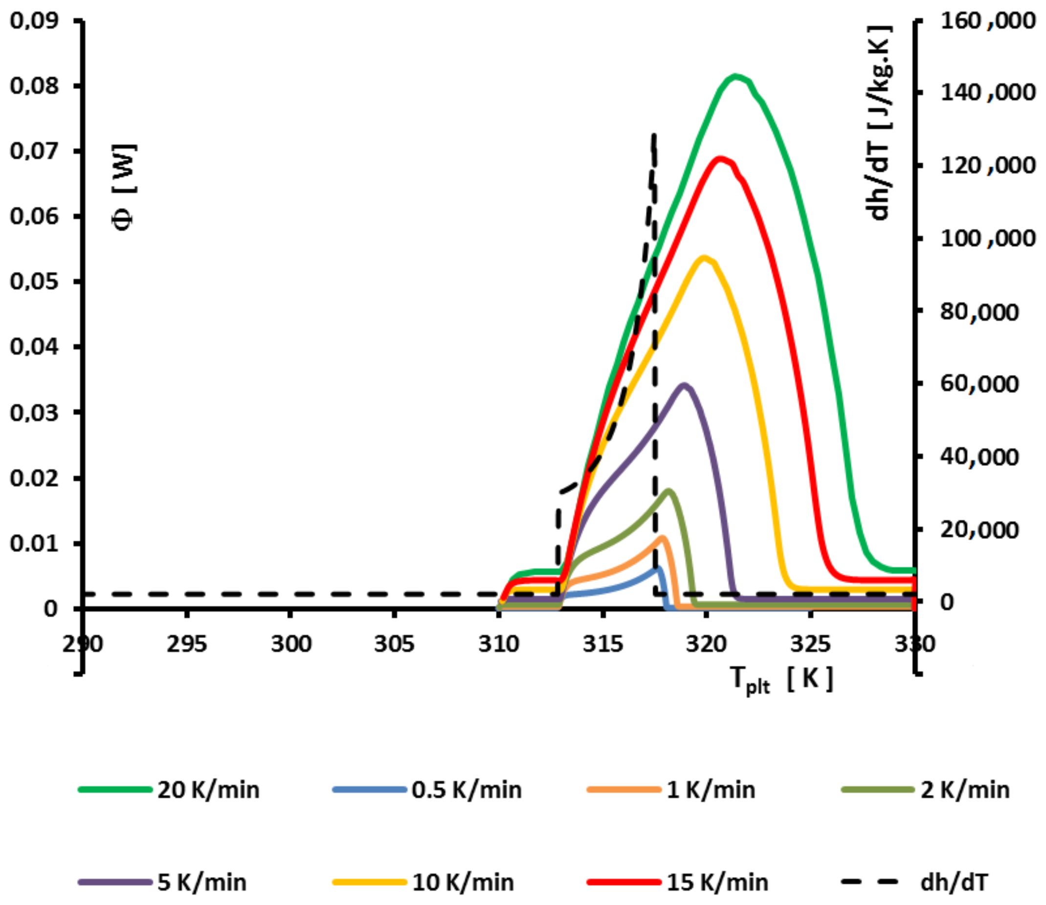
4.4.4. Determination of the Liquidus
If it is relatively easy to determine the solidus because, at , the melting beginning is detected on the thermogram by the left foot of the peak, it is more difficult to determine the temperature at which disappears the last particule of solid.
In this case, we used a similar method as the one presented for the saline solutions to determine
: the extrapolation to the heating rate
= 0. As we can see in
Figure 30, where we present thermograms at different heating rates, for
= 0.8. If we join the points of the top of each thermogram, we obtain a curve which is not a perfect straight line but which can be extrapolated on the zero line to
. As for the saline solutions if it is possible to locate the inflexion points on the right part of the peaks (which corresponds to
the time where melts the last particule as explained in
Section 4.2), we can also plot a curve whose extrapolation gives also
.
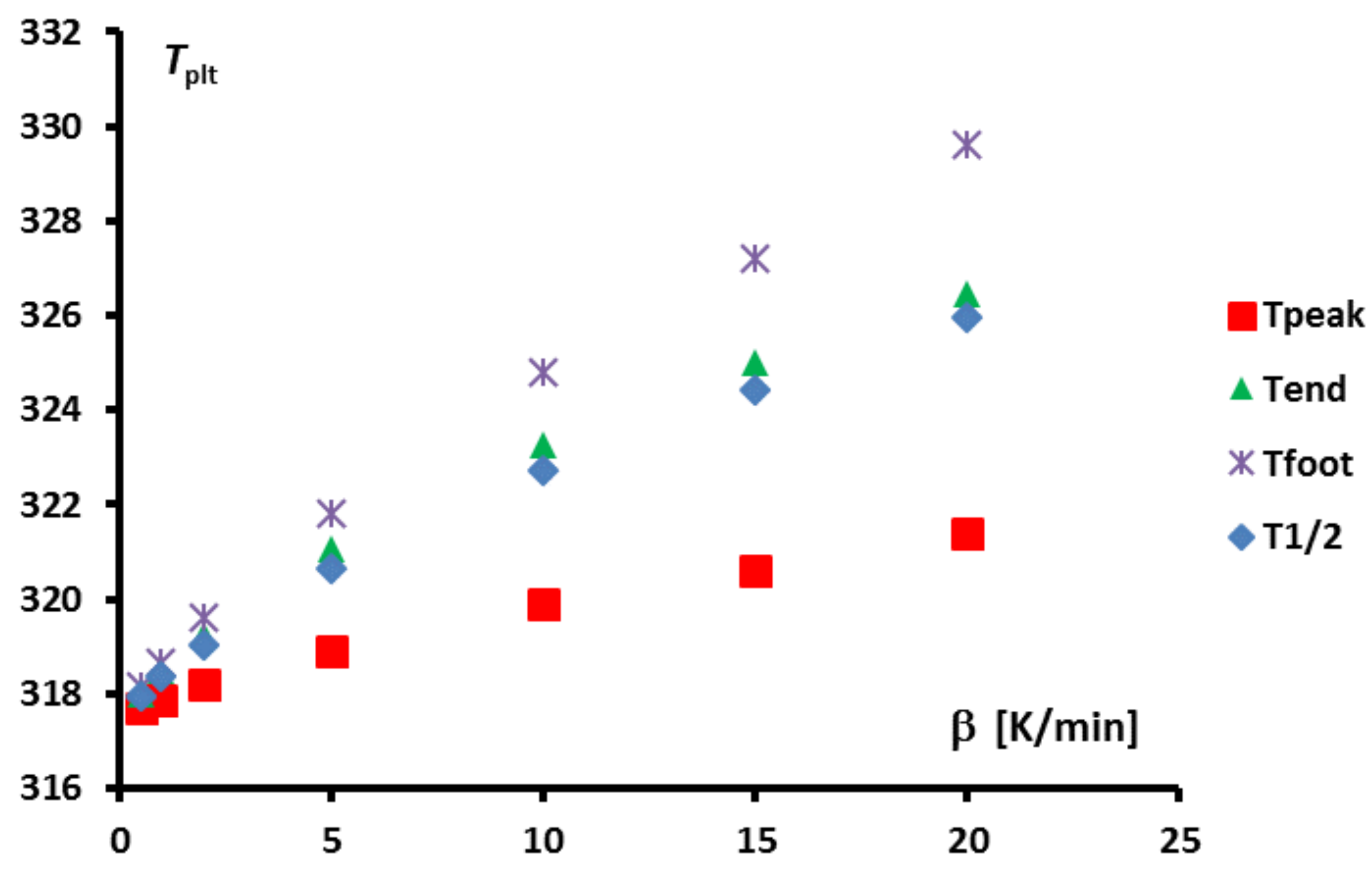
However, in certain cases, it is not always possible to locate correctly these points. For example, in
Figure 26, the points of the top are rather characteristic of the solidus than of the liquidus. It is why, we have defined other points which could be characteristic of the end of the peak. In
Figure 2, we have defined, in addition to the temperature
and
, the temperatures
which is the temperature where we calculate the half height of the peak and
the extreme end of the peak. When
all these temperatures tend to
. It is the case illustrated in
Figure 31. In the two
Figure 30 and
Figure 31, we determine a limit at
= 317.5 K in conformity with the phase diagram of
Figure 25a at the concentration
= 0.8.
In fact, this last method is general and might be used with aqueous solutions (to determine ) or with pure substances (to determine ).
Although we have not studied the accuracy of this method to give the liquidus temperatures, which depends on the form of thermograms, we may think we do not let ourselves be fooled by the peak width to determine this temperature (or the difference ) and this should determine a more correct phase diagram.
4.5. Case of Special Materials
4.5.1. Microencapsulations
Some PCM are microencapsulated and mixed with polymers, plaster or mortar. It is for example the case for PCM incorporated in building construction materials. The microencapsulation avoids leakage at the melting of the PCM. As the size of the particles containing the PCM is very small (less than 1 micron), it is possible to have a sample, even of a few tens of mg which is well homogeneous.
Therefore, all the analyses outlined in the previous chapters can be applied. The difference is that the latent heat of melting only affects the part of the PCM volume (usually less than 15%). However, the height of the melting peak will not be proportional to that of the pure PCM because heat conduction must be considered throughout the sample. The model is the same but with a latent heat reduced to the fraction of the useful PCM.
However, it is possible, when comparing the thermograms with those of pure macroscopic PCM, that one does not have the same form, indicating a solubility of the products of microencapsulation preparation (coacervation?). We have seen that low concentrations of solutes can strongly deform the shape of the thermograms and consequently widen the interval of thermal storage [
17].
4.5.2. Composite Materials
To apply our results to composite materials (see for example [
18]), it must first be checked that cell-size samples tested in the calorimeter can be considered as homogeneous. Secondly, the important information will be given during the change of state of the polymer and not in the “sensible” temperature range where the measurement of the specific heat is less discriminating. Again, the area of the peak is proportional to the amount of the only product that melts.
The comparison of the shapes of the thermograms of the melting of the pure macroscopic polymer and the composite materials will give an indication of the possible contamination of the polymer by the reinforcing elements. The method developed in
Section 4.2 should give an idea of the total concentration of dissolved products.
As for a possible melting temperature distribution (MTD) [
19], it seems necessary to go through a model (if possible already validated) to construct the enthalpy function
h. As for the case of binaries with solid solutions (see
Section 4.4), the value of
is given in a temperature range (plus possibly a rounded part at the beginning of the melting in case of solutions). We have seen that the peaks are enlarged, but their width, depending on the heating rate and the sample mass, is not representative of the melting temperature range. It is possible that the methods explained to determine solidus and liquidus temperature could be applicable to determine the range of the melting temperatures (and not the exact distribution). If the model of MTD is referred by parameters, perhaps it would be possible to determine them applying a reverse method as presented below in
Section 5.4.
5. Methods to Rebuilt
5.1. RRT Method
Among the various Tasks and/or Annexes from the International Energy Agency (IEA), Task 42/Annex 24 devoted to “Compact Thermal Energy Storage / Material Development for System Integration” has participated in the development of a Round Robin Test (RRT) in order to propose a fair comparison of different DSC analysis.
The main goal is to measure the melting enthalpy, and to determine the behavior of the PCM during fusion and crystallization [
20,
21]. A protocol has been defined and tested by several teams, all over the world, using different calorimeters on different substances.
It is particularly insisted on the procedure of calibrations of calorimeters. For each experiments it is optimized the mass sample and the heating rates to be chosen to obtain thermograms permitting to evaluate the melting temperature of the latent heat as close as the true values.
The remaining apparent “hysteresis” is questionned [
22] as we made above.
5.2. T-History Method
The main seminal idea of this method is to have the possibility to test “real” materials, which are often heterogeneous. The principle of the method [
23,
24] is to compare the temperature evolution inside a reservoir containing the PCM with a reference one (usually water). Supposing an homogeneous temperature and assuming that thermal transfers can be written as convective ones, an energy balance permit to retrieve the latent heat [
25,
26,
27].
5.3. STEP Method
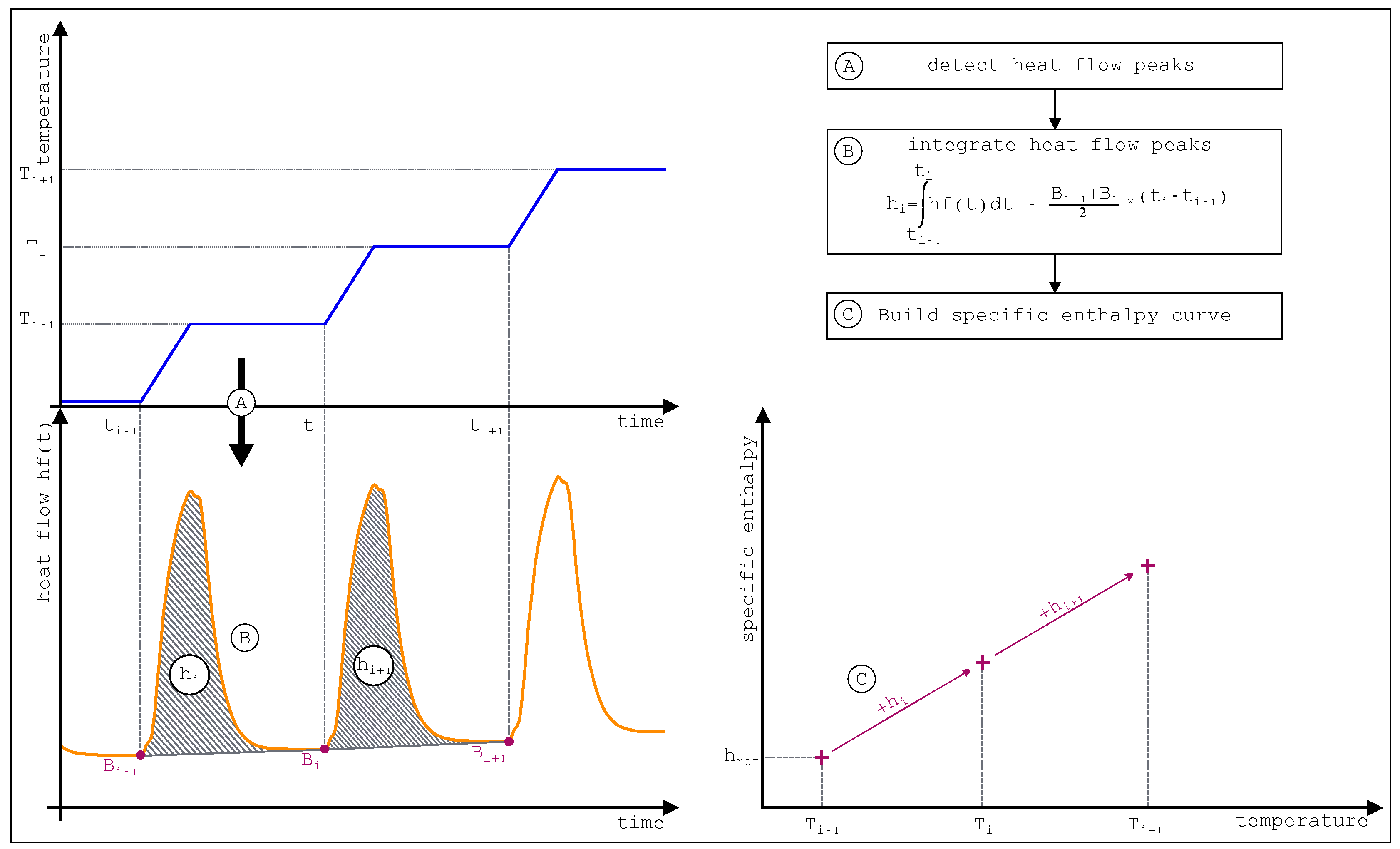
As previously presented, dynamic DSC mode can be carried out relatively quickly but is (apparently) strongly dependent on sample mass and velocities. To overcome these feature another DSC mode has been introduced named “STEP method”. This measure consists in heating the sample and the reference stepwise in a temperature interval. Between each interval, an isothermal level is programmed in order to ensure the thermal equilibrium in each furnace and avoid thermal gradient within the cell.
The three general stages of the STEP method are presented
Figure 32. The thermal load apply to the cell and the reference (
Figure 32 part A) gives rise to the thermogram presented (
Figure 32 part B). Integration of each heat flow peaks allows then to build the specific enthalpy curve (
Figure 32 part C).
STEP method has been used for PCM mixture characterization such as commercial paraffin [
29] and salts hydrates [
30,
31,
32]. It has also recently been applied to the studied of semi clathrate hydrates with progressive dissociation [
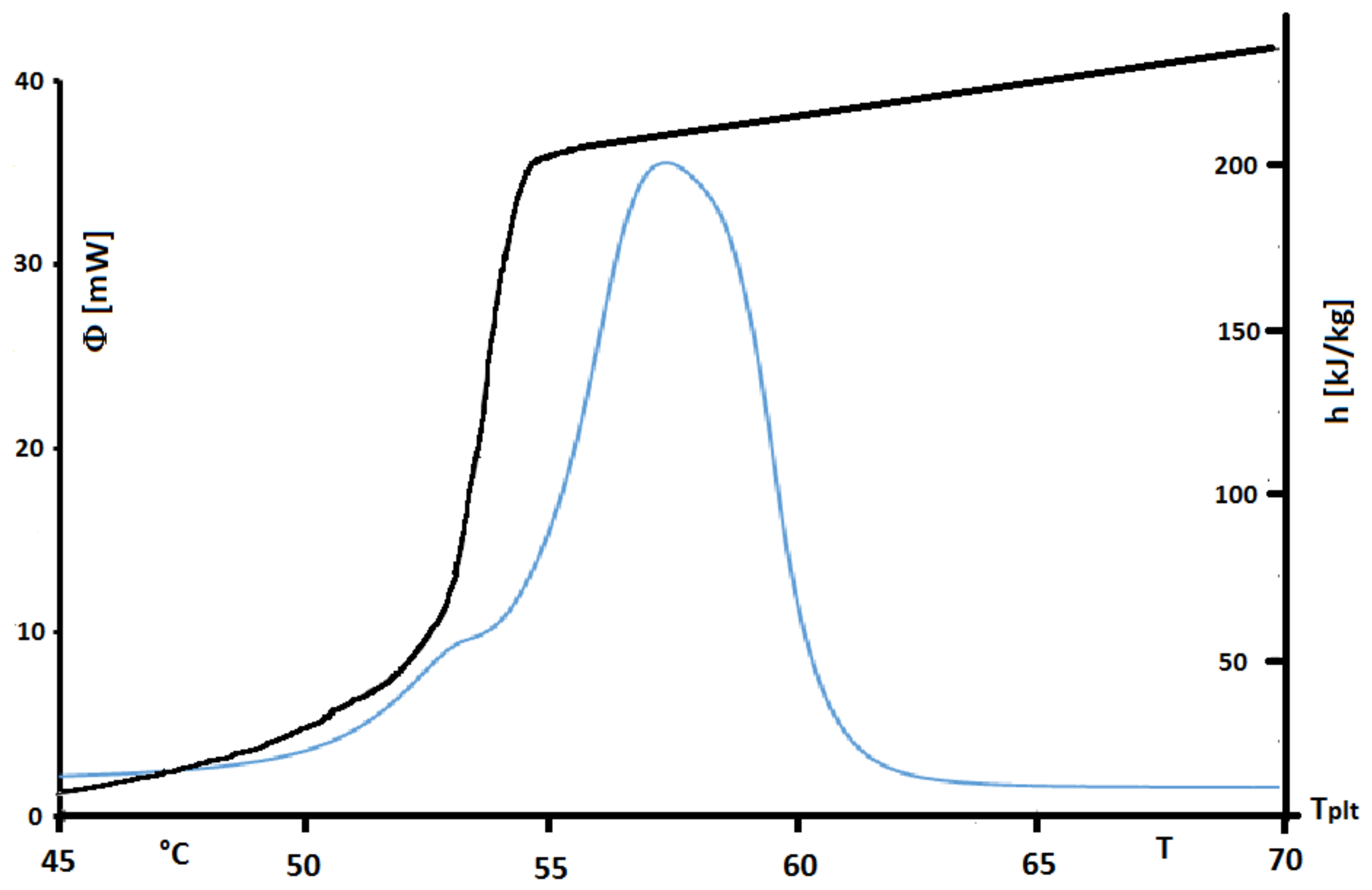
31]. Main advantages and drawbacks are inherent to the method, while isothermal stages allows to prevent of thermal gradients within the cells and the determination of enthalpy curve it also lengths the experiment in an important way. It is also essential to notice that the uncertainty in temperature is confined within the step size and thus increase with it. Recently a sample of commercial fatty acid has been studied in our laboratory. These mixture are easily obtained with high purity laboratory grade. However the use of this compound as PCM in large scale thermal storage system requires the use of industrial product. One of these industrial compound has been tested using STEP method and the result are presented in
Figure 33. Isothermal steps have been done every 0.25
C with heating/cooling rate of
. Treatment process follows the stages presented
Figure 32.
The found value of
h presented in
Figure 33 emphasizes the non-purity of the sample. Unlike a pure substance where enthalpy variation in phase change occurs at constant temperature, that of industrial grade fatty acid occurs over a temperature range, between 50
C and 55
C, which is characteristic of a mixture.
However, in this
Figure 33 we present also the corresponding thermogram for a steady heating at 2 K/min. We perfectly observe that the peak of the thermogram has a temperature range higher than the true temperature range of melting. Indeed this observation is in conformity with our conclusion for pures substances or solutions. We can also conclude that the STEP method is more adequate to give the actual enthalpies functions. Its inconvenient is that the durations of the experiments are very long. It is why, we present another method by inversion.
5.4. Inversion
The numerical model that we presented in
Section 3 enables us to simulate a calorimetric experiment. Based on a complete description of the system (geometry, thermophysical properties) and the solicitations imposed (boundary conditions), the model is able to calculate the evolution of all characteristic quantities and finally to produce a calculated thermogram.
The characteristic parameters of the system are numerical values that are used in the different expressions of the model, such as for example
,
and
of Equation (
18) and that we will group together as a parameter vector
. If we note
the response of the model
relative to the parameters
, we can symbolically write
the operation of direct resolution. It is assumed, of course, that the model is validated by experience, i.e., that under well controlled conditions (i.e.,
known with precision) the model allows to obtain a response
close to the experimental one
.
In the case of inversion, we will use the direct model in order to determine the vector
from a measurement
, i.e., carry out the symbolic operation
. Obviously, the expression
is generally inaccessible and it is then necessary to use an iterative algorithm to obtain an estimate of
. Thus, starting from an initial guess
, one build a suite of solution
that gradually improves the solution. The qualitative assessment of “proximity” is in fact a quantitative criterion that most often corresponds to the least-squares objective function:
In the favorable case we therefore have . The estimation is considered acceptable when criterion falls below a selected value. The heuristic used for the -correction at each iteration defines the inverse method.
To cite just three examples, genetic algorithms, the simplex method and descent methods such as those described by Levenberg and Marquardt are used. The genetic algorithms [
33,
34] are working on a population of potential solutions, which limits the risk of converging to a local minimum. It also has the particularity of not requiring the calculation of the gradient of the objective function
in the research space, which is time-consuming and often requires approximations that degrade the quality of the solution (and may prevent convergence). The simplex method [
35] is equivalent to approximating
locally and correcting the potential solution
in the direction of decreasing
. Finally, the Levenberg-Marquardt [
36,
37] method derives from the gauss-newton method and approximates
in the neighborhood of
by a quadratic function that determines the optimal descent direction.
For illustration, we present here some results obtained for the identification of the
function for
solutions [
13]. The thermodynamic model is slightly more complex because it takes into account the eutectic transformation that occurs at around
. The estimations were made on samples of increasing concentrations (
,
,
and
) with masses varying between 9 mg and 10 mg. For each sample, two experiments were carried out at 2 K/min and 5 K/min.
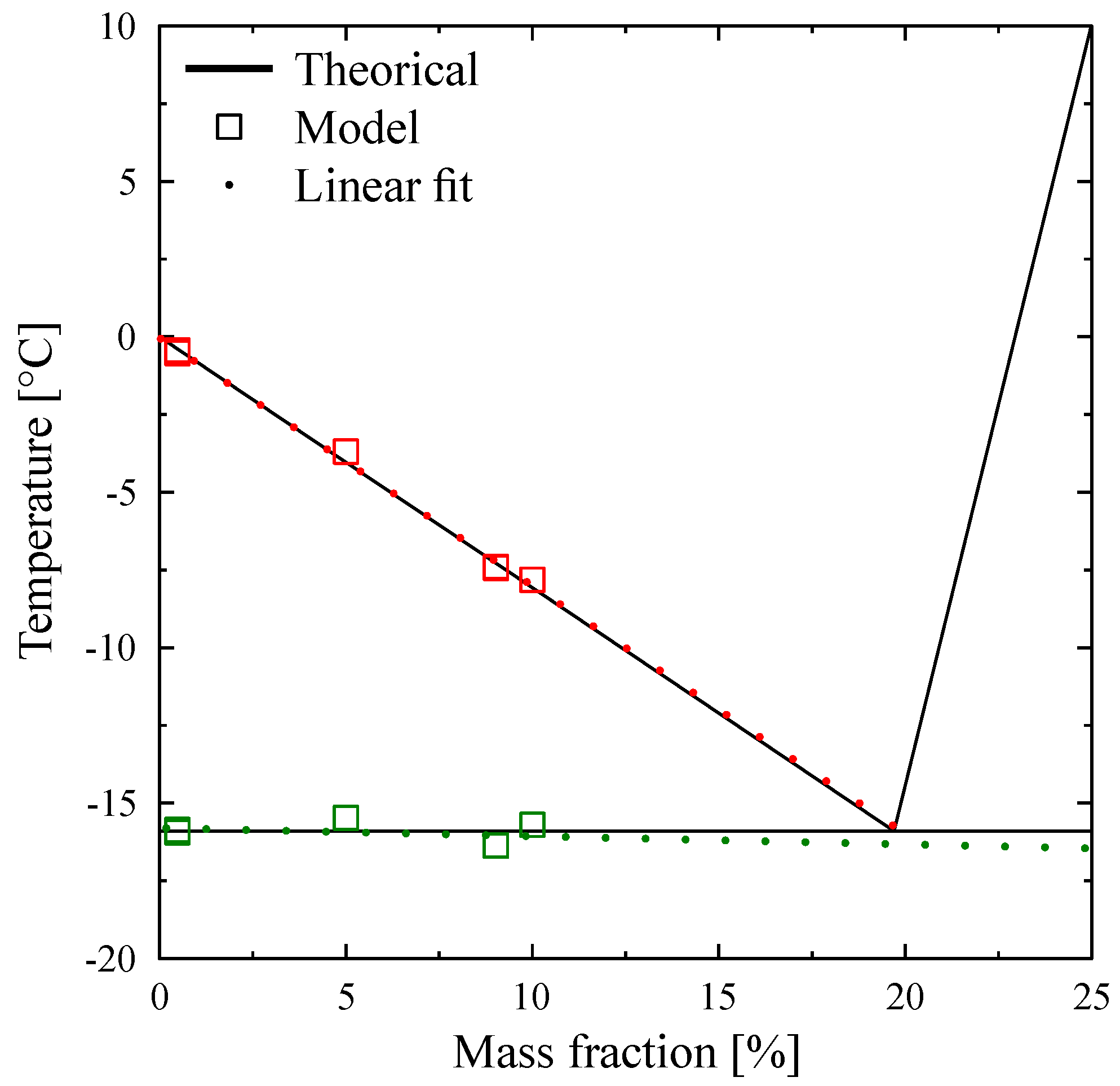
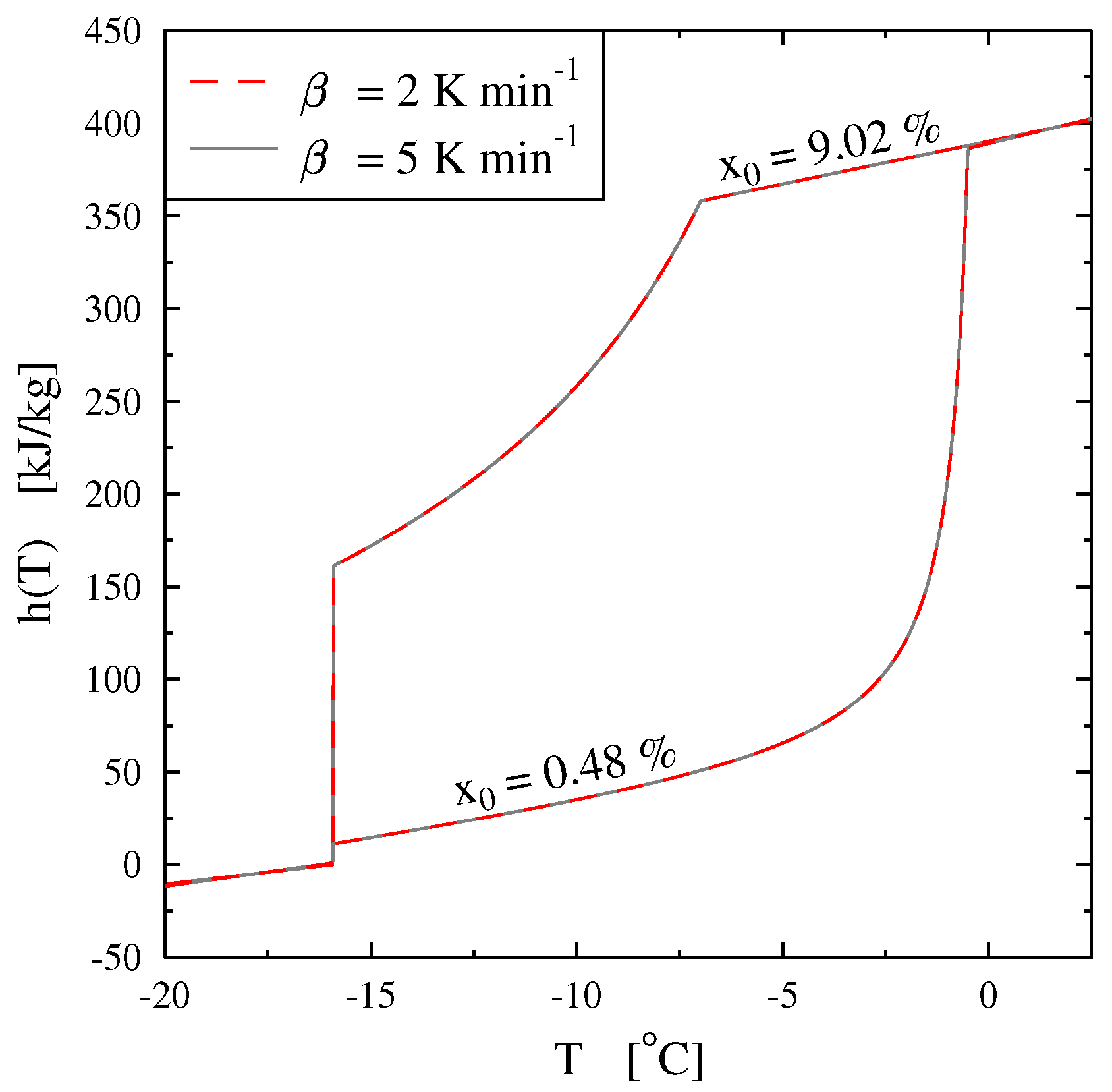
Figure 34 shows the estimated
for concentrations
and
and for both heating rates. It is confirmed that this method permits to obtain the function
independently of the heating rates, which is in agreement with thermodynamics. From the respective estimations, it is possible to position certain characteristic temperatures (
and
which must be in conformity with the phase diagram of the solution. Thus, on
Figure 35 we present the phase diagram resulting from the literature (continuous line) on which we have pointed the identified temperatures. There is a very good agreement which shows the relevance of the inverse approach for the characterization of phase-change materials by calorimetry.
6. Difficulties in the Management of Supercooling
For many years our Laboratory has studied the supercooling phenomenon. We have particularly studied the case of the supercooling of dispersed liquid within emulsions. Our book [
38] contains a great number of references.
The main characteristics of the crystallization of the supercooled liquids are:
the supercooling (i.e., the difference between the melting temperature (or ) and the temperature of crystallization ), depends on the volume of the sample: the smaller the volume of the sample is, the greater the supercooling is.
due to the nucleation phenomenom which governs the appearance of the first nucleus causing the crystallization, this change of state is an erratic phenomenon governed by statistical laws.
The consequences deduced from the item 1. is that, to complete information with emulsions (liquid droplets whose volume is of the order of a few ) we observe very important supercoolings (15 K for paraffins, 39 K for water, and more than 100 K for certain organic substances). We can predict that the volumes of the samples studied in calorimeters which are of the order of few give smaller supercooling (1–2 K for paraffin, 15–18 K for water or aqueous solutions, 30–40 K for certain organic compounds , a few K for molten salts or several tens of K for hydrated salts...). However, these supercoolings detected by DSC are larger than those observed in the volumes of the industrial tanks (a few liters or ).
The consequence of the item 2. is that the crystallization begins at a point (probably at a point near the surface because in this region the temperature is the lowest) and propagates. Considering the erratic character of the nucleation evoked above, this point has not only an unpredictable position, but it is not reproducible from one crystallization-melting cycle to another. The crystallization is an exothermic phenomenom and the temperature quickly increases up to the equilibrium temperature. So, the sample is made of a part of solid (we can calculate its total amount but not its localization: for example, for water, it appears only 1.25% of ice per K of supercooling) and the liquid is at the melting temperature ( for a pure substance or given by the phase diagram if a solution is concerned). Therefore, it seems not so simple to model the consecutive crystallization especially if natural convection is concerned.
An example, where the supercooling and the erratic character of the crystallization must be taken together into account concerns the storage of energy using aqueous PCM inside nodules (about 8 cm in diameter) contained in a tank crossed by the fluid carrying the heat energy [
39,
40]. Although nucleating agents are used, the supercooling is only reduced to about 2 K (and not canceled) and it is necessary to take into account a probability of crystallization of the PCM and the kinetics of solidification at each point of the nodule.
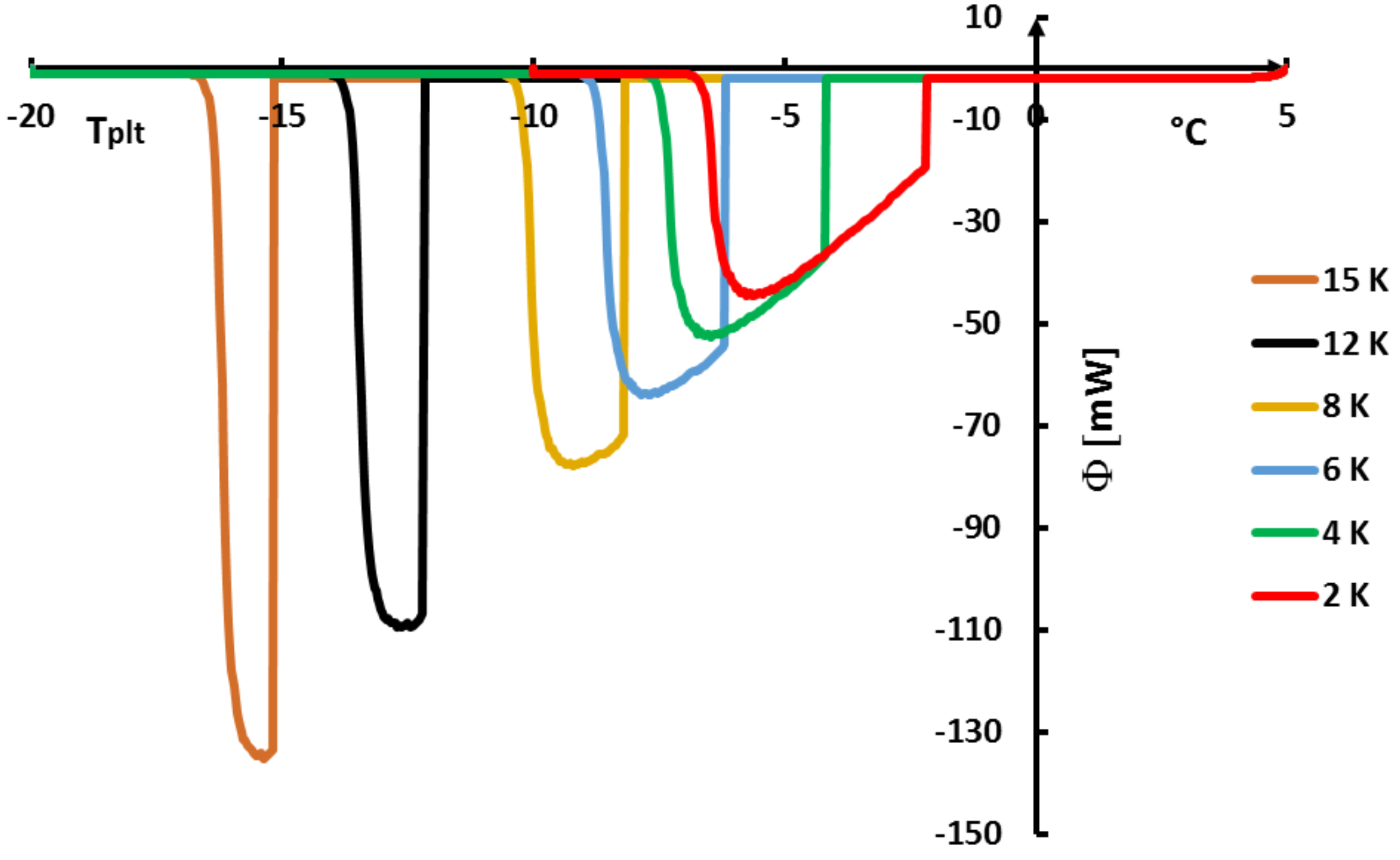
In
Figure 36, we present [
41] the DSC curves obtained with water for different supercoolings
using the same model as above with Equation (
2) where
and (
3) to (
5). The difference is that, at the time
of the crystallization when the temperature is
, it appears the solid phase (ice) and the remaining liquid part
has a temperature which increases to
.
is given by [
39,
40]:
and in this case
= 97.5% for
= 2 K and
= 81.2% for
= 15 K.
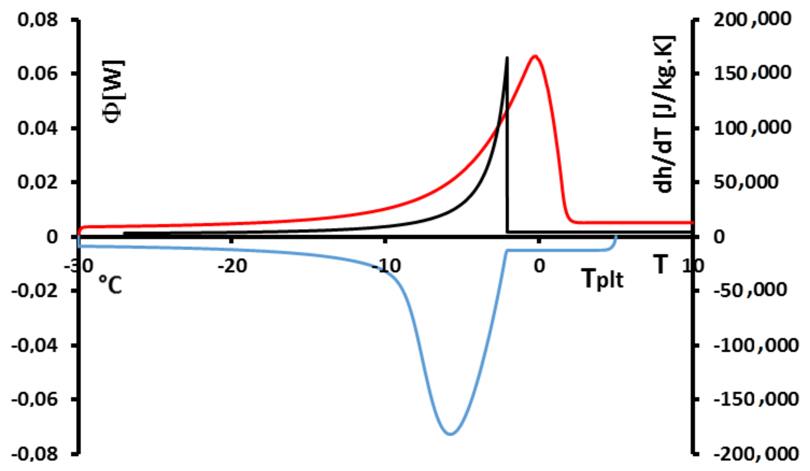
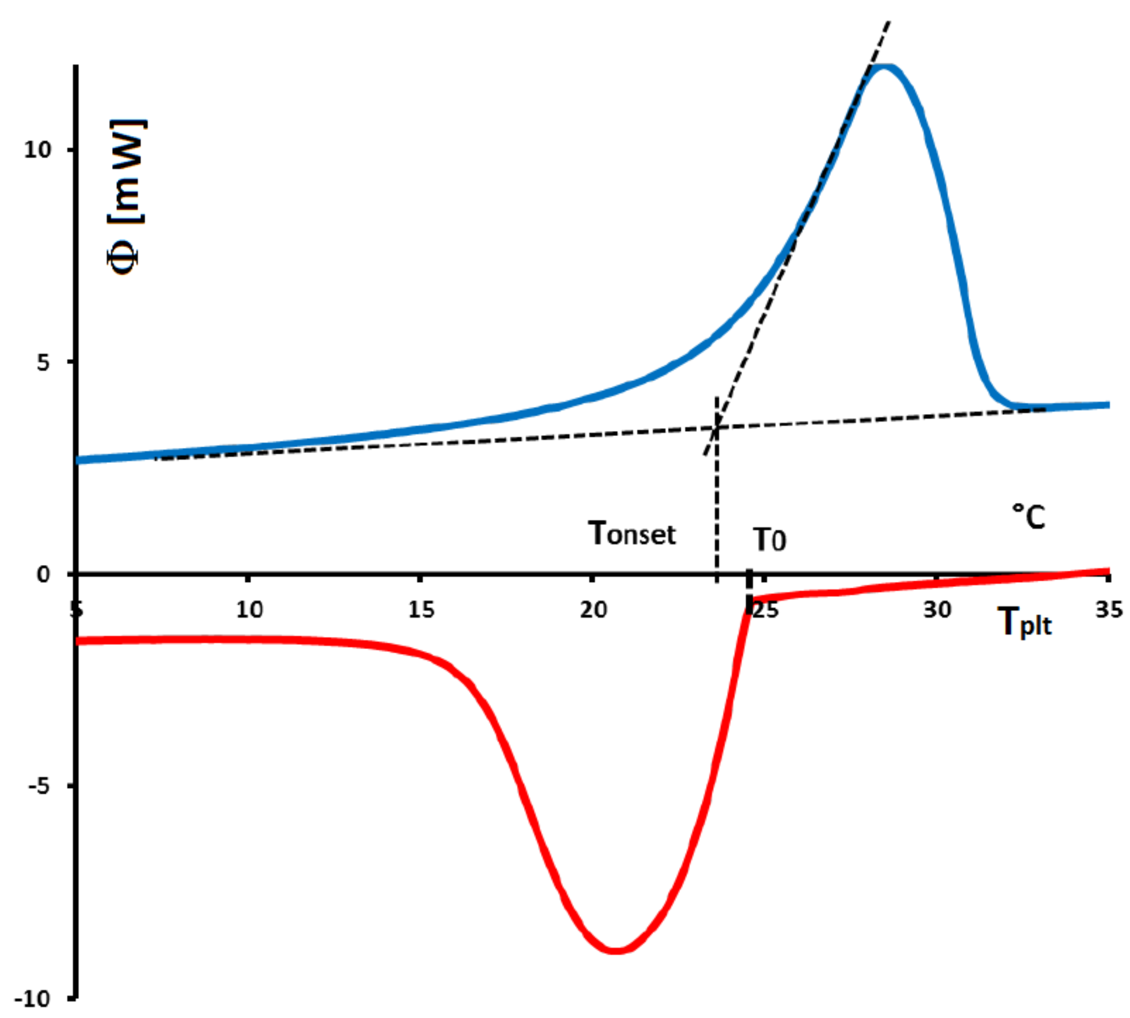
In
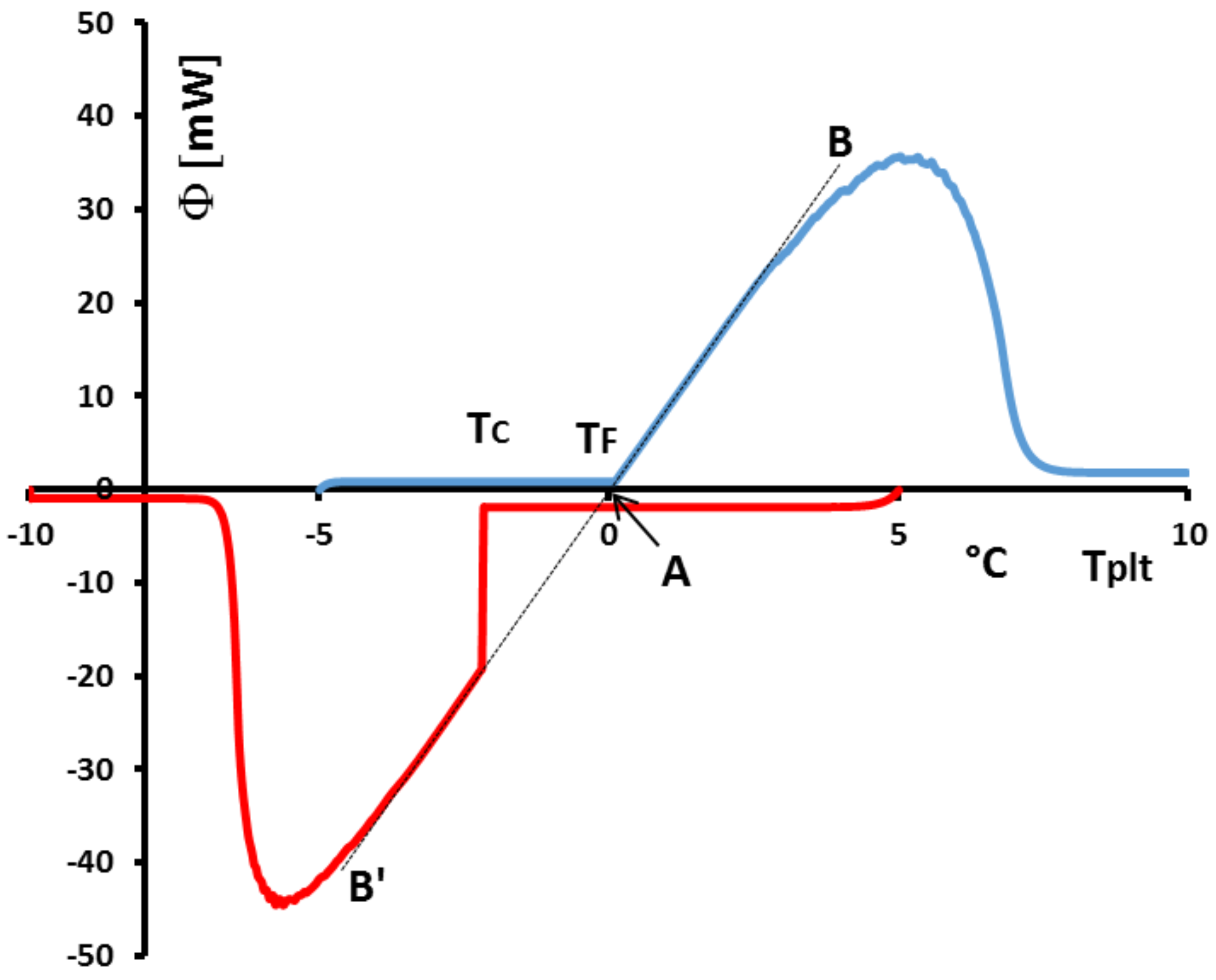
Figure 37, we analyse the particular case of a low supercooling of 2 K (in red). We have also drawn (in blue) the DSC curve for the corresponding melting at the same heating rate. We particularly observe that if we plot the lines of greater slope of the melting (AB) and of the crystallization (AB’), they are aligned as we can see with the corresponding black dotted lines. These dotted lines intercept the zero line at 0
which is the melting temperature of the investigated water with the calibration described above in
Section 4.1.6. However, such an experiment, with the two lines of greater slope (AB) and (AB’) which align, shows that the calibration in temperature is the same on heating and on cooling. This is important, because if we notice that practically all liquids present a supercooling giving a crystallization temperature not completely predictable, as mentionned above, a calibration on cooling is not directly feasible. If the questionned two lines of greater slope are shifted, a correction can be easily programmed taking into account the difference of temperature at the interception with the zero line.
Another problem linked to the phenomena observed on cooling is related to the incorrect use of the temperature
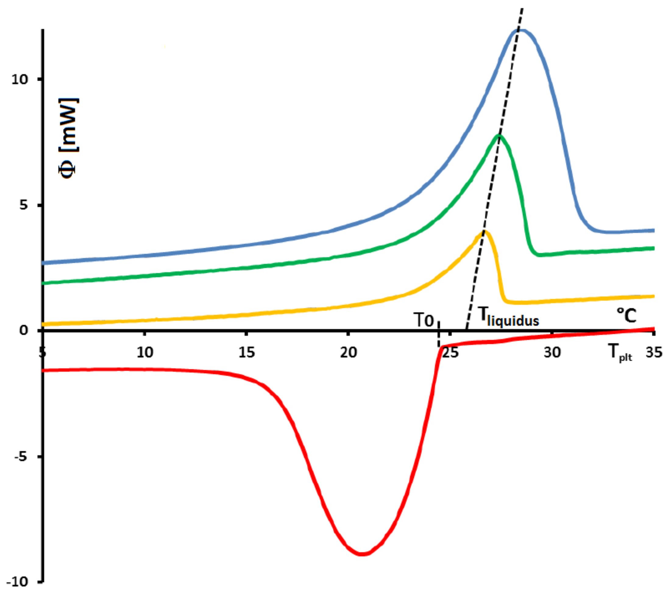
with solutions. In
Figure 38 we present the heating and the cooling at 5 K/min of a commercial PCM. The shapes of the thermograms indicate that it is about a solution. In this figure, if we compare
the temperature of crystallisation detected at the beginning of the peak and the onset temperature
classically determined and if this temperature is considered to be the melting temperature, there is a major problem because it would be concluded that the crystallization temperature would be higher than the melting temperature.
It is absolutely forbiden by the Second Law of Thermodynamics (the variation of the Gibbs free energy
G would not be negative).
However, if we use the method (explained at the
Section 4.2), with different thermograms (see
Figure 39) at different heating rates, consisting in extrapolating the line joining the top of the peak to the zero line we can determine the true value of the temperature of the equilibrium
for such a solution. In this case, the Second Law is satisfied since
.
n.b.: Indeed, as a rule of thumb, it is not the presence of supercooling that leads to the conclusion of an hysteresis phenomenon but the spreading of the DSC curve. Furthermore, even if supercooling leads to a non-symmetrical behavior between the fusion and the solidification, it will only affect the beginning of the crystallization (and certain PCMs, as the paraffins, present a very small supercooling of the order of one K), and not the rest of the DSC curve. No real hysteresis phenomenon could be withdrawn directly from the thermograms, even in case of supercooling.
7. Conclusions
In this paper we have considered that, obviously, the physical (thermodynamical) laws are the same whatever the volume of the sample may be. So, even when the samples studied by calorimetry are relatively small (a few ), the thermodynamic laws of melting (solid-liquid equilibrium) and the physical laws of the conductive heat transfers are both taken into account.
The detailed study of the melting of a pure substance indicates that the heat flow rate which constitutes the thermogram is representative of the phase change considering the temporal evolution and not the linear evolution of the temperature of the plate of the calorimeter. Indeed, inside the cell, the phase change at constant temperature occurs on an interface which evolves with time from the walls of the cell to its center. At no moment there exists a particle melting at a temperature different from , contrary what is asserted by previous studies stating that the sample would have a homogeneous temperature almost equal to the one of the plate.
Through this study on pure substances, whose the local melting is at a fixed temperature, several observations and conclusions have been drawn. Firstly, there are always temperature gradients inside the sample during phase change, whatever the heating rate and the mass. Secondly, this thermal gradient leads to a differentiated temperature field between the interface temperature and the plate’s one. Consequently, the DSC curve is spread over time and “appears” to be spread also with the temperature (of the plate). However, this spreading is not representative of the phase transition and seems to depend on the heating rate and mass sample. Thirdly, and because of the previous remark, it is not relevant to directly integrate the thermogram, even non-dimensionnalized, to try to build the enthalpy function. Fourthly, the attempt to reduce the thermal gradient by lowering the heating rate can anyway give an enlarged enthalpy function, especially if larger masses are used for the samples. Meanwhile, the limit of the noise to ratio signal raises the uncertainties. Fifthly, the so-called hysteresis phenomenon is only due to an incorrect interpretation of the thermogram and does not exist in reality.
Nevertheless, it does not mean none information can be taken from such a model on pure substances: we have demonstrated that as it is always possible to determine the melting temperature, possibly with a modified procedure of calibration, and the associated latent heat with a good approximation.
For the saline solutions, we can also explain why the thermograms are more enlarged than the thermodynamic temperature range and over the liquidus temperature. This enlargement depends on the heating rates and the classical onset temperature has no meaning. A procedure to determine the temperature of the liquidus is detailed. The results are applied for the particular case of the small concentrations. We found that to use the thermograms as if a pure substance were concerned corresponds to very small concentrations (≤0.01% in moles). For higher concentrations, the thermograms are not compatible with a validation of the onset temperature. Although the errors are very small, a significant bad evaluation of the melted quantities is predictable.
Our model can be extended to the binaries with solid solutions. The case of ideal solutions is detailed. The methods explained with pure substances or saline solutions are applicable with success to determine the temperatures of the solidus and the liquidus and potentially the phase diagram.
With some additional commentaries it is suggested how to analyze or predict calorimetric analyses concerning microencapsulated PCM or composite materials.
Then, the different methods known to determine the function
: RTT, T-history, STEP or inversion technics are analyzed. These methods are generally used to characterize materials for the fine-tuned modeling of transformations, particularly in thermal storage applications [
42]. For many years, our Laboratory mainly implements these two last methods (STEP and inversion technics). Obviously, it is noticed that an additional experimental effort is required in the case of the STEP method and a numerical effort in the case of inversion.
Finally, DSC curves, on cooling, indicate a supercooling by the delayed crystallization. It is explained how the results can, or not, be extended to industrial tank containing PCM. A consequence of this study, is the demonstration of a procedure to calibrate the calorimeter on cooling.


