Multi-Agent System for Demand Prediction and Trip Visualization in Bike Sharing Systems
by
 , , and
Álvaro Lozano
1,* ,
,
Juan F. De Paz
1,
Gabriel Villarrubia González
1 ,
,
Daniel H. De La Iglesia
1 and
Javier Bajo
2
1
Faculty of Science, University of Salamanca, Plaza de la Merced s/n, 37002 Salamanca, Spain
2
Department of Artificial Intelligence, Polytechnic University of Madrid, Campus Montegancedo s/n, Boadilla del Monte, 28660 Madrid, Spain
*
Author to whom correspondence should be addressed.
Appl. Sci. 2018, 8(1), 67; https://doi.org/10.3390/app8010067
Submission received: 15 December 2017
/
Revised: 1 January 2018
/
Accepted: 2 January 2018
/
Published: 5 January 2018
(This article belongs to the Special Issue Multi-Agent Systems)
Abstract
:Featured Application
The main application of this work is the analysis and prediction of the demand in bike sharing systems using their open/private data. A multi agent system is proposed and a case study is conducted using the data of a bicycle sharing system from a middle size city.
Abstract
This paper proposes a multi agent system that provides visualization and prediction tools for bike sharing systems (BSS). The presented multi-agent system includes an agent that performs data collection and cleaning processes, it is also capable of creating demand forecasting models for each bicycle station. Moreover, the architecture offers API (Application Programming Interface) services and provides a web application for visualization and forecasting. This work aims to make the system generic enough for it to be able to integrate data from different types of bike sharing systems. Thus, in future studies it will be possible to employ the proposed system in different types of bike sharing systems. This article contains a literature review, a section on the process of developing the system and the built-in prediction models. Moreover, a case study which validates the proposed system by implementing it in a public bicycle sharing system in Salamanca, called SalenBici. It also includes an outline of the results and conclusions, a discussion on the challenges encountered in this domain, as well as possibilities for future work.

1. Introduction
There is a consensus in the literature [1,2] which states that bicycles are one of the most sustainable modes of urban transport and they are suitable for both short trips and medium distance trips. Riding a bicycle does not have any negative impact on the environment [3], it promotes physical activity and improves health. Furthermore, its use is cost-effective from the perspective of users and infrastructure.
Moreover, due to the increased CO2 levels, the European Union and other states are taking measures to reduce greenhouse gas emissions in every sector of the economy [4].
These facts explain the growing popularity of sustainable means of transport such as bike sharing systems. From 1965 when they came into use in Amsterdam to 2001, there were only few systems around the world. Bike sharing systems (BSS) began to spread in 2012, when their number increased to over 400 [5]. By 2014 this number had doubled [6] and nowadays there are approximately 1175 cities, municipalities or district jurisdictions in 63 different countries where these systems are in active use, according to BikeSharingMap [7].
Bike sharing systems allow users to travel in the city at a low cost or even for free. They can pick up a bicycle at one of the stations distributed across the city and leave it at another. These systems have evolved over time [8] and today the vast majority include sensors that provide information on the interaction of users with the system. However, the management of these systems and the data collected by them, is often poor and as a result the numbers of bicycles available at stations are not sufficient.
These are the reasons as to why bike sharing systems should be improved with data produced by the systems themselves. They should include predictive models for user behaviour and demand, which will notify the system administrator of the stations where more bicycles are required for satisfying user demand. This will also allow to set up new stations in places where the demand is high or, on the contrary, to close down the stations at which the demand is too low.
This article presents a multi-agent system which collects bike sharing system data together with other useful data. The system uses these data to create demand prediction models and to offer services through an Application Programming Interface (API), used as a prediction and visualization tool. This application has two main functions: (1) it visualizes historical data including the flow of bicycles between stations and (2) it predicts the demand for each station in the system. In order to perform the prediction of demands, the system includes different regressor systems based on previously collected data. The system has been tested with data provided by Salamanca’s bike sharing system (SalenBici) getting successful results regarding to the demand prediction. This will provide the administrator with more information about stations and users in the system as well as useful data for the bike reallocation process.
This work is structured as follows: Section 2 overviews the state of the art of current works and techniques involved in bike sharing systems and prediction models and points to the current issues in this field. Section 3 describes the proposed system architecture and provides a concise description of every part. Section 4 presents a specific case study: we test with the bike sharing system called SalenBici of Salamanca to validate the system proposed. Finally, Section 5 provides insights about the results and conclusions of this case study and points out research challenges for future works.
2. Background
2.1. Bike Sharing Systems
All bike sharing systems operate on the basis of a common philosophy, their principle is simple: individuals use bicycles on an “as-needed” basis without the costs and responsibilities that owning a bicycle normally entails [9]. Figure 1 shows a classical bike station, where there are free docks and available bikes to rent within a station map of Madrid’s Bike Sharing System called BiciMad. As shown on the map, the bike sharing system offers a wide list of stations located across the centre of the city.
Peter Midgley indicates in his study [3] that bike sharing systems can be categorized into 4 generations depending on their features: (1) First generation bike sharing systems: the first generation of bike sharing systems was introduced in Amsterdam (1965), La Rochelle (1976) and Cambridge (1993). These systems provided totally free bicycles which could be picked and returned in any location. The vast majority of these systems were closed due to vandalism. (2) Second generation: this generation tries to solve the drawbacks of the previous one. In this case, the systems had a coin deposit (like the supermarket trolleys) but they still suffered from thefts due to the anonymity of the users. (3) Third generation: this generation uses high tech solutions including electronic locking docks, smart cards, mobile applications, built-in GPS devices in the bikes and totem applications. (4) Fourth generation: it is still in the process of development, this generation includes movable docking stations, solar-powered docking stations, electric bikes and real-time system data.
This last generation of systems includes a new scheme named dock-less bike sharing solution which reuses the first-generation philosophy: free bicycles around the city. However, in this case, they are equipped with a GPS tracker and they can be found and rented through a mobile application. This kind of systems are quite spread nowadays in China and they are arriving to cities like Singapore, Cambridge and Seattle through enterprises as OFO [10], Mobike [11] and Bluegogo. Nevertheless, these bike sharing systems may suffer from vandalism and other problems already presented in first-generation. Some of these big enterprises—such as Bluegogo [12] in China—has recently gone bankrupt due to financial problems.
Furthermore, these bike sharing systems present other kind of operating diagram that varies from the one based on stations. In consequence, there are huge differences regarding to the data processing. This work focuses on systems based on stations which will be deeply discussed.
Concerning Third and Fourth generations of BSS, there are some common issues that will be described in detail in the following section.
2.2. Bike Sharing Main Issues
Current literature lists factors that influence the success of bike sharing systems, these include the built environment, psychological factors related to the natural environment, as well as the utility theory. This last reason focuses on providing users with the best quality of service, by addressing any issues encountered in the bike sharing systems. Vogel et al. [9] describes three main issues in bike sharing systems; their design, management and operation. The authors distinguish three categories:
- Network design and redesign issues: These decisions address issues related to the initial design of the system, they consider the topography, traffic and equity of stations located across the city [10]. The amount of docks and the number of vehicles at each station are important factors in this category. These issues occur not only in the initial design but also in the subsequent use of the system: long term corrections of stations could be done thanks to the insights provided by the data analysis tools created with the information generated using the system.
- Incentivizing users to balance the system: These decisions are related to operational matters and they aim to mitigate the main operational problem: the shortage event [13] that occurs when a customer wants to pick a bike from an empty station or return it to a station whose docks are occupied. Users are incentivized to occupy the stations with available bikes and docks. These incentives could involve changes in the pricing policies or even a reservation station system that ensure availability at the final station. This kind of incentives could be implemented in systems that operate on a pay-per-use basis but they are more difficult to implement in systems with a fixed quota per year.
- Operational reallocation issues: This category also focuses on an operational aspect, known as the commutation pattern in bike sharing systems. There are specific bike station usage patterns, for example, in the mornings the stations located on the outskirts of cities are empty because many people travel to the city to work. On the other hand, the stations in the city tend to be full in the mornings [14]. As we mentioned previously, the empty and full stations must be balanced by system administrators and this reallocation must follow a specific strategy that is based on the demand predicted for each station provided by prediction demand models. They must additionally use a reallocation algorithm which minimizes the total cost of managing bike fleets. In this case, there are two more problems: the prediction engine and the optimization algorithm used to reallocate the bikes. This work addresses the prediction problem but does not discuss the reallocation strategy.
Now that we have identified the main issues that should be considered in these systems, in the next paragraphs it will be described how a visualization tool is used to solve the problems related to the first category. We will also focus on the third category, especially on the demand prediction models. Moreover, we will show works in the literature that regard demand prediction models and the kind of data have been employed to build them.
2.3. Bike Demand Prediction Models
In the literature, we can currently find numerous works on station demand prediction. Some address the problem from a data mining point of view [15] with an exploratory data approach [16]. Afterwards, works like Kaltenbrunner et al. [17] show how to implement prediction models based on time series analysis methods like Auto-Regressive Moving Average (ARMA).
Subsequently, in May 2014, Kaggle [18], a known machine learning competition platform, launched a competition about the Washington D.C. BSS. In this competition, participants were asked to combine historical usage patterns with weather data in order to forecast bike rental demand in the Capital Bikeshare [19] program in Washington, D.C. Due to this competition, a lot of researchers began to work in prediction models to obtain the forecast of bike demand in stations.
Romain et al. [20] use the data described above to in the analysis of several regression algorithms from state of the art. They applied these algorithms to predict the global use of the bike sharing system. They establish baseline predictors as references of performance and apply Ridge Regression, Adaboost Regression, Support Vector Regression, Random Forest Regression and Gradient Tree Boosting Regression. They perform predictions up to 24 h ahead and their study covers the whole system instead of each station independently. Patil et al. [21] also present prediction models about the total number of bikes rented per hours in the system in their work. The authors compare Random Forest, Conditional inference trees and Gradient Boosted Machines. Wen Wang [22] perform a great comparison of the approaches proposed by other authors, while others like Lee et al. [23], Du et al. [24], Yin et al. [25] among others in their dissertation. This work offers a great overview of past research works on this topic.
Previous works are interesting if we want to look at total demand in the entire bike sharing system but nowadays it is possible to obtain station data from Open Data services [26,27] and private services [28] which can be used to build prediction models for each station and forecast the demand. This will allow to provide useful information for a further bike reallocation strategy and avoid shortages.
Diogo et al. [29] present an interesting work where they achieve the previous two objectives: prediction models for each station and a rebalancing algorithm. The data employed in this work provided information about Chicago BSS [30] and Washington [31] bike systems and it was related to the trips travelled in the system. In the system proposal section of this work it will be explained what kind of information is contained in trip data. The authors propose the use of Gradient Boosting Machines, Poissson Regression and Random Forest to build prediction models and they use a variant of the Vehicle Routing Problem (VRP) with the framework Jsprit to perform the reallocation strategy. The authors do not provide any open source code nor an in-depth explanation.
In this work, we will employ some well-known methods which have also been used in the described literature, to predict the demand at each station and provide useful information for the subsequent reallocation task, which will be studied in a future work.
3. Proposed System
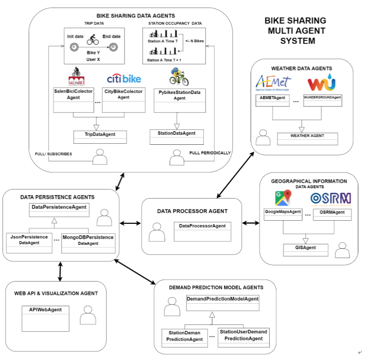
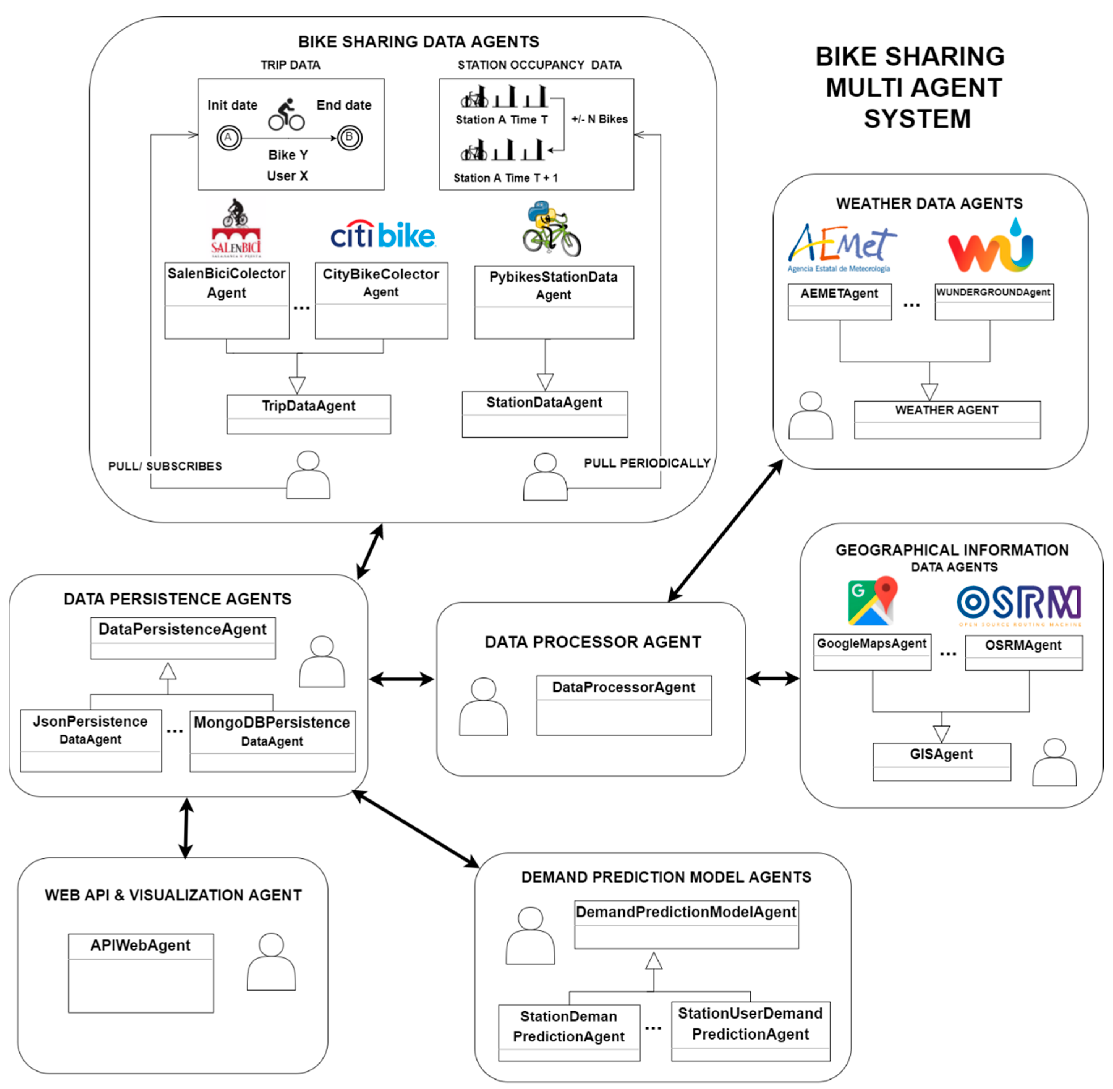
This section details the proposed multi agent system (MAS) and presents a general diagram of the system’s architecture which is shown in Figure 2. Literature shows that multi agent systems have previously been employed in similar tasks like taxi fleet coordination [32] where they offer an ideal solution to abstract away issues of the different existing platforms and communication protocols. The system is divided into the following groups of agents: bike sharing data agents, weather data collector agents, geographical information agents, data persistence agents, demand prediction agents and API agents. Several multi agent platforms such as SPADE [33,34], JADE [35], PANGEA [36,37], AIOMAS [38] and osBrain [39] were evaluated and osBrain was finally selected for this system because of its ease of use. Furthermore, it is implemented in Python (like SPADE and AIOMAS) and it is in continuous development nowadays.
Each agent group will be described in detail in following sections, including issues encountered, techniques, developed processes and decisions taken.
3.1. Bike Data Sharing Agents
Bike Data Sharing Agents are responsible for obtaining data from the BSS, which usually offers two kinds of data:
- Station information: It indicates the total number of available docks and bicycles at each station at a given time, that is, the current situation at the station. This data is usually available and provided to the end users in order to keep them informed about the stations with available bicycles. If this data is periodically polled, pickups and returns at each station can be calculated regularly. This kind of information only provides us with knowledge about variations at each station without specifying the flow of bikes from one station to another or data regarding the users involved in these changes. It is usually provided through an API in real time by a great amount of BSS, so much so that there is a project called PyBikes [27,40] which unifies the access to this information through a common API for a large number of current BSS. The multi agent system presented in this paper includes a station data agent that periodically collects this information for the target BSS.
- Trip information: This sort of information is not commonly published but it is usually available in csv files offered every month as open data [41]. It is related to the trips recorded by the BSS: a user picks a bike at a specific station at a given time and later returns it at another station. This kind of data discloses more details as it provides insights on the flow of bikes between stations and the users who perform the trips recorded in the system. This information will be especially useful for the visualization tool and demand prediction in BSS with registered users (occasional users are not included). There is a trip data agent in the system that asynchronously gets data from a public or private data source.
This group of agents sends the collected information to the Data Persistence Agent, which is in charge of storing the raw data that will later be processed by the Processor Agent.
3.2. Weather & Environment Data Agents
Weather & Environment Data Agents obtain the weather data requested by the Processor Agent, they provide historical weather data for the requested dates and locations which will later be merged with trip or station data. These agents will also provide weather forecasts to Prediction Model Agents; they need this information when making predictions for a specific station at a given time.
The weather data obtained by these agents is daily data on: minimum, maximum and average temperature, wind speed, rain and minimum and maximum pressure. There is a common base agent to provide this information and specific data agents responsible for implementing that functionality for each weather provider such as Wunderground [42] or Aemet [43].
3.3. Geographic Information Data Agents
The Geographic Information Data Agents obtain the geographic location and the distance between stations as well as the altitude of each station. A base agent offers services related to this information and a specific agent implements this functionality with different data providers such as Open Source Routing Machine (OSRM) or Google Maps. This information will be stored and employed later by API agents in the visualization tool. This information will also be useful for future works where a reallocation bike strategy must be calculated.
3.4. Data Processor Agents
Data Processor Agent processes the data obtained by Bike Sharing Data agents. Additionally, this agent will request the weather agents to provide information regarding the bike sharing data dates and it will clean and merge that information with the previously obtained bike sharing data. This process will be executed periodically in order to obtain all the recent information that is pending to be processed.
Since different kinds of information are obtained by the bike sharing data agents, the data processor agent is capable of perform two different data processing workflows. The selected workflow will depend on the type of input information: trip data information or station data information. As it has been pointed out previously, the output data obtained by processing either kind of input information will be different and will be employed differently depending on the case study.
Figure 3 shows the flowchart of the data processor agent in detail. This agent will perform different data processing methods based on the input information and then it will send the results to the data persistence agent, for storage. Every workflow and their included sub processes are explained in-depth below.
3.4.1. Trip Data Workflow
First of all, trip information is received as input data. A process of dropping outliers is performed for Trip Data. Trips that lasted less than 2 min are dropped out because they are considered an attempt of using a bike which is malfunctioning, so it is taken and immediately returned to the same station.
Besides that, the processor data agent requests the weather data agent to provide weather data in the range of dates of the input data. The information provided by the weather agent is cleaned and if there is no weather data for data records, a lineal interpolation is performed in the data. This information is merged with the input information. Then new features are added to the current dataset. These features divide dates into years, months and days of the week, day of the month, hours and other derivative features as seasons, weekends, holidays (obtained for each country with the library Workalendar library [44]). At this point, the received information is cleaned and merged with extra information. The next step involves splitting the information by station in the system and creating departures and arrivals. For each station in the system, that had the same station of origin are converted into departures and all trips with the same station as their destination are converted into arrivals.
Once this is executed in every arrivals/departures dataset, the information will be grouped by a period T and the total number of arrivals/departures in each period T is summed. An additional step is performed, this is necessary in order to generate records for the periods for which no information on trips is available, periods of the day when the number of trips is zero. This process is called adding no activity data. Finally, the information is sent to the persistence data agent that will store it for further utilization by the model prediction agent.
3.4.2. Station Data Workflow
This process is slightly different from the previous one but they share common steps in the sub processes. The information received is related to each individual station in the system, the difference between consecutive records will show the arrivals or departures of bikes in the system. From the beginning the data is split into arrivals and departures at each station that is part of the system. Then the previously mentioned process of cleaning and merging weather information is performed. Next, the process of adding information on dates is also performed. Finally, the data is grouped by a period T, no activity data is added and the information is sent to the persistence data agent, as in the previous data process. Once the data is grouped and cleaned it is ready to be used by the Predictor Engine in the making of demand forecasts for each of the stations in the system.
3.5. Demand Prediction Agents
These agents are responsible for carrying out two main tasks: generating the prediction models for each station as well as providing demand forecasting for a specific station, at a concrete time. These agents will run periodically generating new models if new data is available. The demand prediction agent will request the cleaned data to the data persistence agent and it will generate the following prediction models using the machine learning library Scikit-learn [45].
3.5.1. Regression Models Employed
Regression models such as Random Forest Regressor [46], Gradient Boosting Regressor [47] and Extra Tree Regressor have been employed as they have obtained the best results in previous studies [22,48,49,50]. In the case study, the tested algorithms and their results are described in-depth. In order to compare the quality of the estimators a dummy regressor has been employed as a baseline regressor, which uses the mean as a strategy for performing predictions.
3.5.2. Model Selection and Employed Evaluation Metric
The evaluation metric selected in this work is the Root Mean Square Logarithmic Error (RMSLE) Equation (1). Although there are many common methods for comparing the predicted value with the validation value, such as Root Mean Square Error (RMSE) or Mean Absolute Error (MAE). However, the metric employed in this problem is RMSLE as suggested by the Kaggle competition.
where is the RMSLE value (score), is the total number of observations in the dataset, is the prediction and is the actual response for , is the natural logarithm of .
The fundamental reason behind this kind of error is that using the logarithmic-based calculation ensures that the errors during peak hours do not dominate the errors made during off-peak hours. Kang [51] discusses why this error is employed in the competition.
3.6. WEBAPI Agent: Visualization and Forecast API and Web Application
This agent will offer access to historical data as well as demand prediction services through a Web Application Programming Interface (WebAPI). Likewise, this agent will provide a web application that will use the previous services to offer information to the BSS operator. The web application will be compound by two main sections:
- Historical data visualization: This section will provide information on the BSS’s historical data. It also offers visualizations of trip data information, permitting the user that is filtering historical data to explore user behaviour between stations.
- Forecasting & Status: this section will show the current status of the system and the demand forecasts for the selected station.
4. Case Study
4.1. BSS SalenBici
The SalenBici System is a bike sharing system located in Salamanca, a medium city with a population of 144.949 according the last 2016 census [11]. Today, this system has 29 stations and 176 bikes throughout the city. The system working hours are: work days from 7:00–22:00 and weekends and holidays from 10:00 to 22:00. Figure 4b shows the station map of SalenBici BSS.
The system operators employ trucks as it is showed in Figure 4a to perform reallocation tasks in the evening, at noon and in the afternoon, thus extra information on the expected demand in the mornings and evenings could be useful for performing the reallocation tasks.
4.2. Data Collection Process
The data collected regards all trips travelled in the system from a station of origin to a final station. In this case the information provided by SalenBici company is trip data, as mentioned previously and it has the following information in the original dataset: (1) Time Start: timestamp of the beginning of the trip, (2) Time End: timestamp of the end of the trip, (3) Bicycle ID: unique bike identifier, (4) Origin Station: origin station name, (5) End Station: destination station name, (6) Origin dock: origin dock identifier, (7) End dock: destination dock identifier, (8) User ID: user unique identifiers.
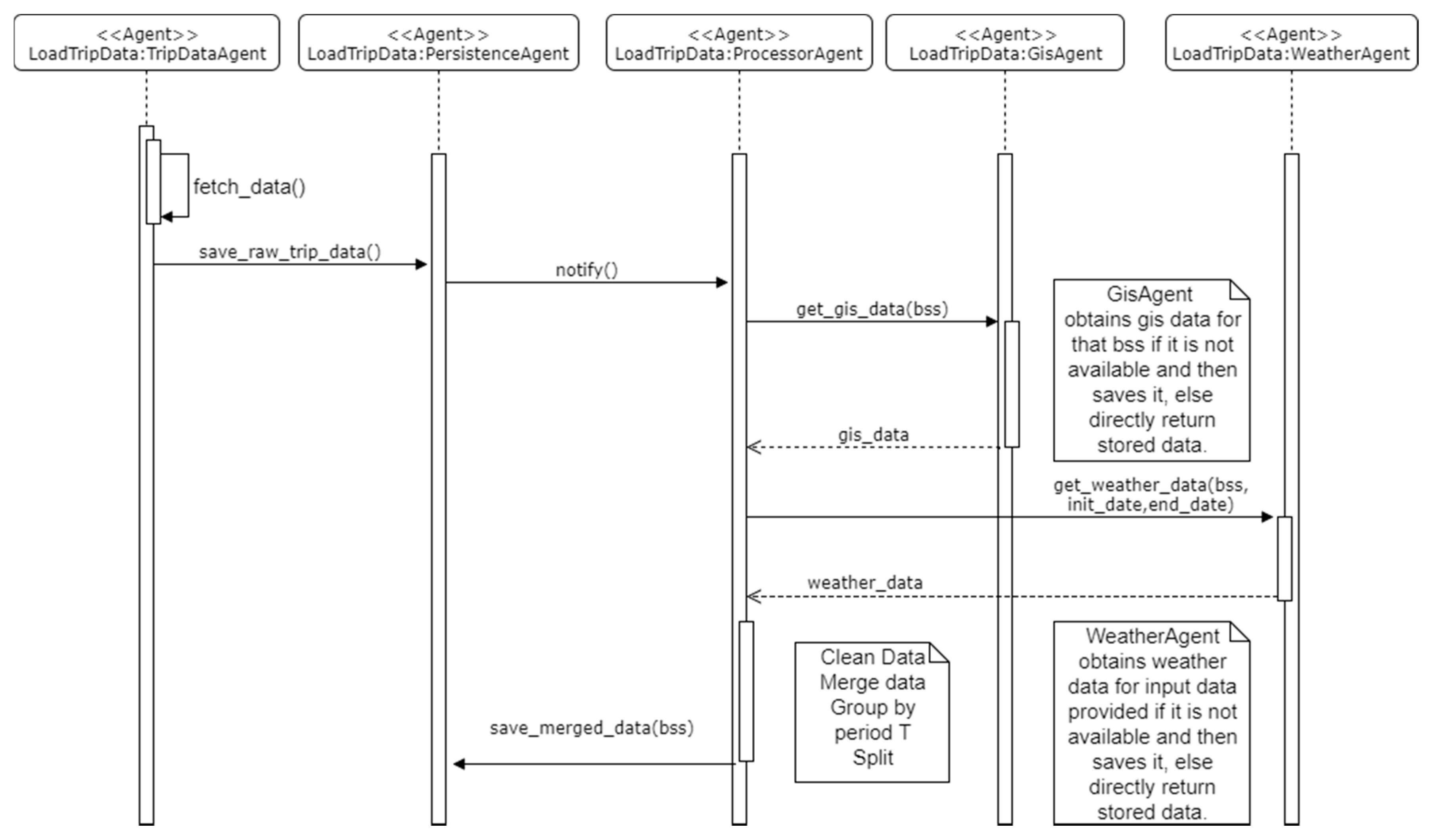
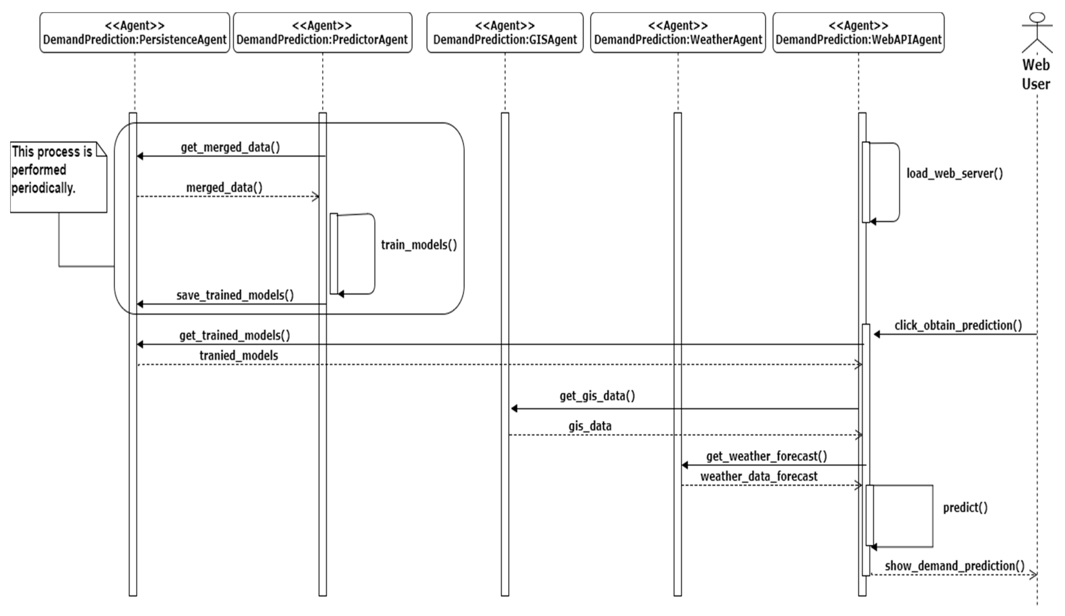
The SalenBici company provided us this information in the form of csv files, one for each year. To process this information, the files were given to the multi-agent system. The trip agent loads all the data from the provided data source, the processor agent is notified by the persistence agent because new raw data is added to the system. The processor agent checks the data and request geographic and weather data from the Geographic Information System (GIS) Agent and Weather Agents respectively. Before these agents respond to the request, they check the availability of data with the persistence agent, if the data is available it is sent immediately. On the other hand, if information is not available it is first collected, saved and then sent to the processor agent. Figure 5 shows a sequence diagram of the activities performed by each agent, the communication between the GIS and weather agents and the persistence agent is omitted for clarity.
After this process, the stored output data contains the following information on arrivals and departures: Year, Month, Day of the Week, Day of the month, week of the year, hour, season (winter, spring, summer or autumn), weekends and holidays as time related information. The information that is available in relation to the weather on a particular day, is the following: the maximum, minimum and average temperature in degrees Celsius, the average wind speed in km/h, the minimum and maximum atmospheric pressure in millibars and the amount of rainfall. We have the total amount of arrivals or departures in the grouped period T is a dependent variable.
Before spawning the predictor data agent in the multi agent system, an exploratory analysis of the processed data was performed. This analysis determined what model should be included in the predictor data agent.
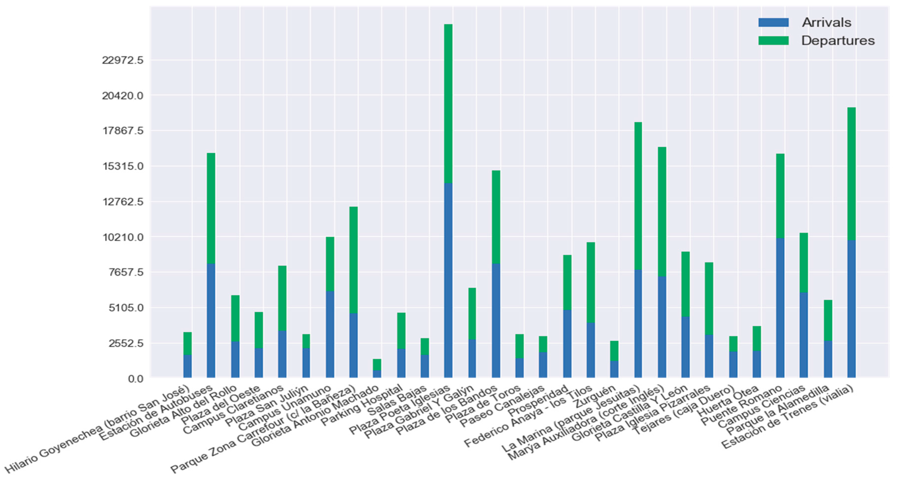
Figure 6 shows the total number of trips loaded in the system, which are divided into arrivals and departures for each of the stations in the system. This data dates from January 2013 until March 2017 a total of 1520 days and we can see a clear difference between the use of stations in the system. There are a lot of stations where the mean of the bike trips is less than 2 events (arrivals or departures) per day. The station with the highest mean is called “Plaza Poeta Iglesias” near Plaza Mayor (the most touristic place in the city of Salamanca), with 15 events per day (arrivals or departures).
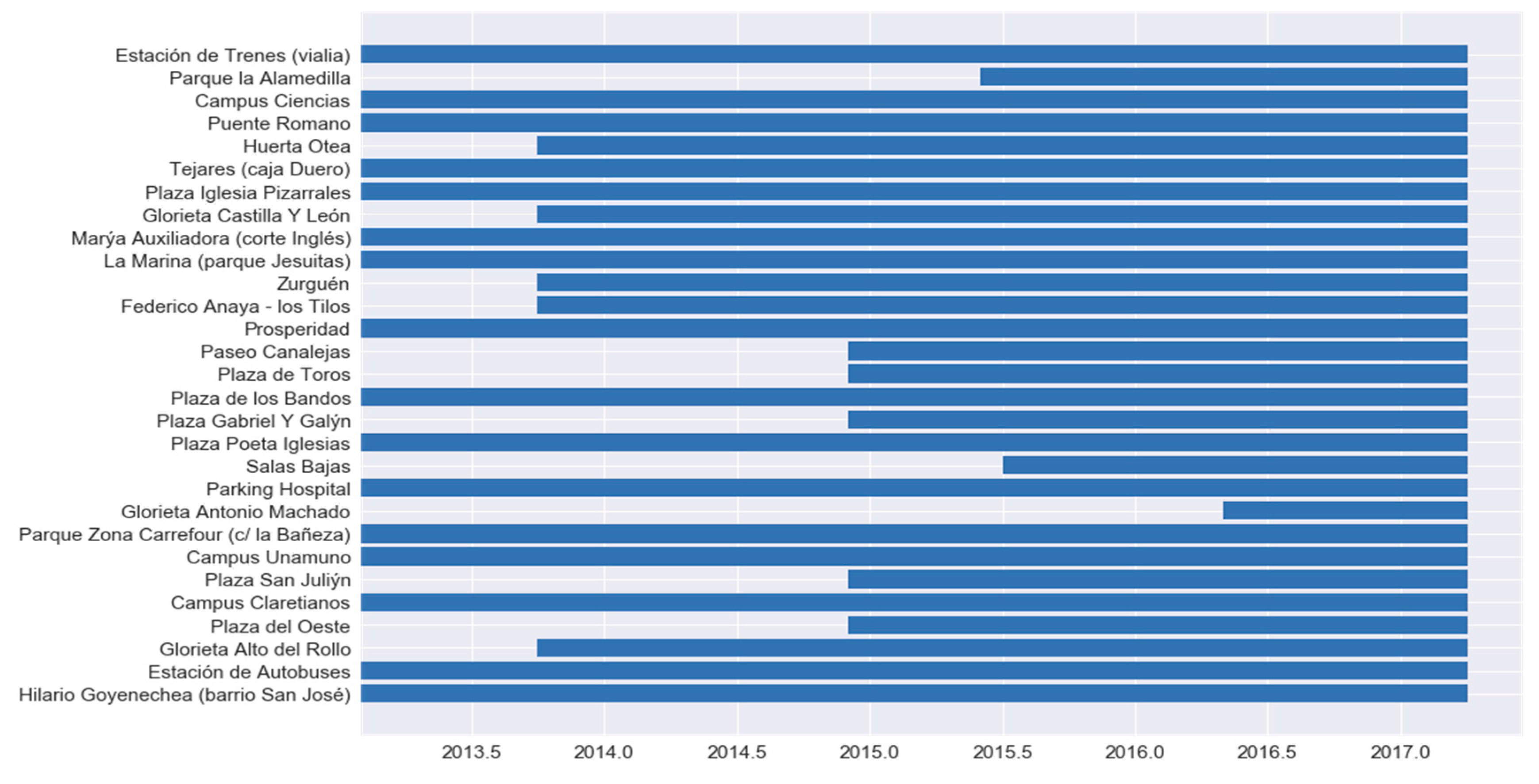
In addition, Figure 7 shows the time period from which each of the stations in the system is active. When reading the total number of trips from the previous figure, it is important to take into account that not all stations have been working since January 2013.
4.3. Model Selection
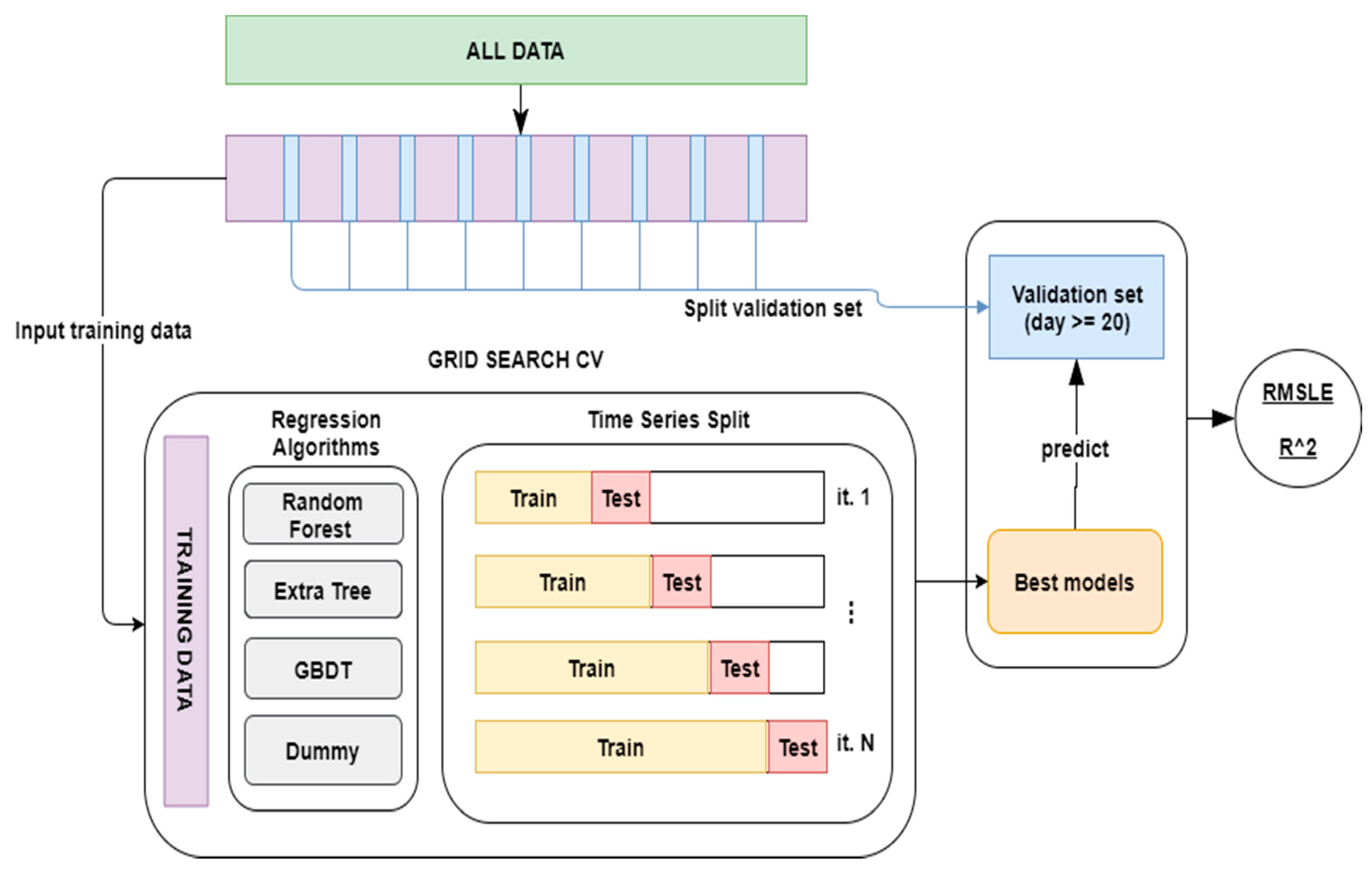
This section describes how the BSS dataset was split and the methodology that was used in order to select the prediction models that will be included in the predictor agent. Like in Kaggle competitions [17], the data have been split into two datasets; a training dataset and a validation dataset. Figure 8 shows schematically how the available data were employed in the training, selection and validation of the models used. In the upper part of the figure, the green part represents the entire dataset. Like in Kaggle competition, a validation dataset is initially extracted and it is formed from the 20th to the end of each month, in the diagram it is represented in blue. The rest of the dataset, (those from the 1st to the 19th of each month), will be used as training data, represented in violet in the diagram. These data will be one of the inputs of the hyperparameter search technique: GridSearchCV [50]. This technique will use the following as inputs: (1) regression algorithms with their corresponding parameter grid; (2) a scoring function, in order to evaluate the input models, in this case RMSLE and R2; finally; (3) a cross validation method, in this case TimeSeriesSplit, a method that is intended specifically for time series and which resembles the usual functioning of a system in production. This method makes it possible to progressively use data from the past for training and use future data for validation, a diagram showing its functioning is situated in the lower part under GridSearchCV, in Figure 8.
The GridSearch method will make all the possible combinations for each algorithm with the provided grid parameters; this will be done by employing the cross-validation method (Time Series Split) and evaluating the trained methods with the provided scoring functions. As the output of this method, models for each algorithm with the best results will be obtained and these will be evaluated with the validation dataset that had been split at the beginning, on the right-hand side of Figure 8. A Dummy Regressor has been added to the models used and was established as their prediction strategy in order to continually predict the average. The regression algorithms as well as the following parameter girds have been trained using GridSearchCV:
- Extra Tree Regressor: learning rate: [0.1, 0.01, 0.001], subsample: [1.0, 0.9, 0.8], max depth: [3, 5, 7], min samples leaf: [1, 3, 5]
- Random Forest Regressor: criterion: [mae, mse], number estimators: [10, 100, 1000], max features: [auto, sqrt, log2]
- Gradient Boosting Regressor: learning rate: [0.1, 0.01, 0.001], subsample: [1.0, 0.9, 0.8], max depth: [3, 5, 7], min samples leaf: [1, 3, 5]
Once the model is selected, the results of the best selected model are validated with the validation dataset that had been split previously. Additionally, the coefficient of determination R2 of the models selected for each station has been calculated.
4.4. Results and Discussion
Next, the results of the RMSLE validation dataset are outlined. The results of the best models selected by the GridSearchCV for each station, are described. Figure 9 shows the results for arrivals and Figure 10 shows results for departures. From these graphs, we can see that regressors tend to have better results than the established baseline. The Random Forest Regressor and the Extra Tree Regressor have the best results.
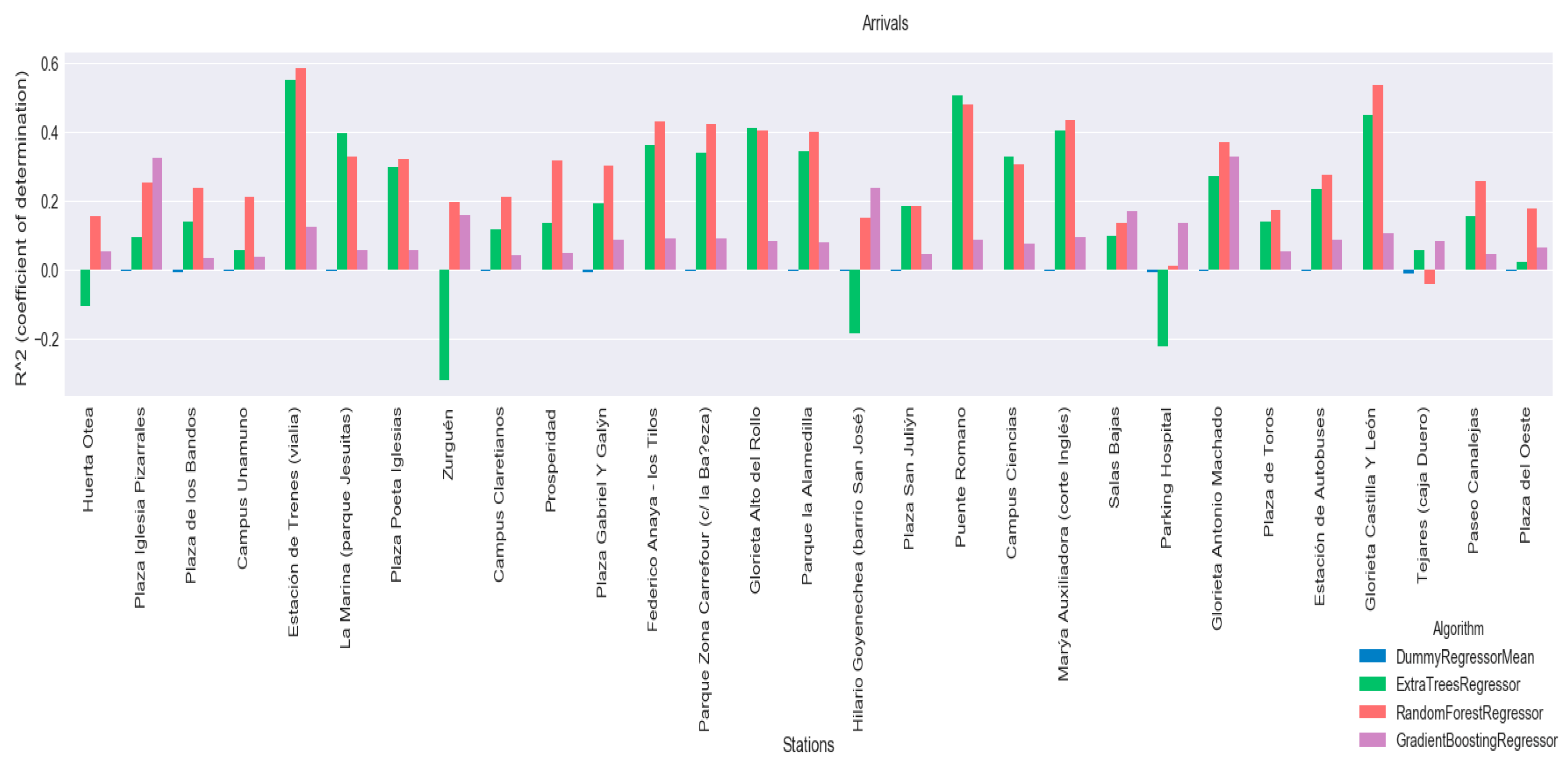
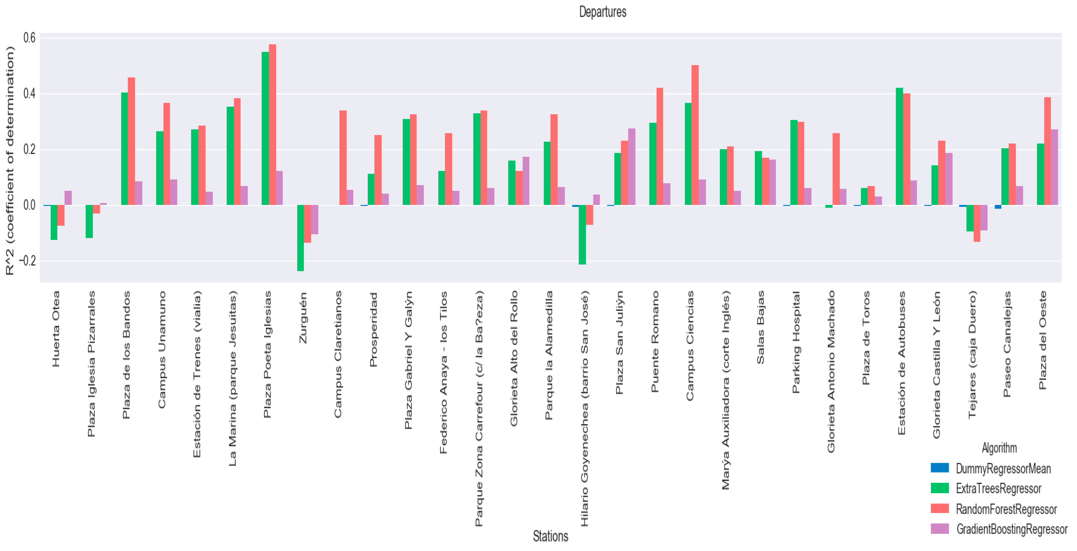
Additionally, the coefficient of determination R2 has been calculated for each of the algorithms, with the aim of using it to select a model that will be included in the predictor agent. The results of the coefficient of determination are shown for each of the algorithms at each of the stations, for arrivals in Figure 11 and departures in Figure 12. Graphically, that the method that performs the best with R2 is Random Forest Regressor, however results will be analysed to see if this difference is significant.
In order to select the best algorithm for all the stations in the system, a statistical Mann-Whitney U test was used. First, the test was done in order to check if one of the algorithms used, functions differently to the rest. The following confirmatory data analysis was applied: considers the median of two equal methods while considers the median of two different methods. As we can see in Figure 13, in the case of both departure and arrival models, the Random Forest Regressor Algorithm has a median that is different to the rest, thus, it could be considered that there is a significant statistical difference. The p-value obtained for the Random Forest Regressor and Extra Tree pair, surpasses slightly the test’s 0.05 significance level, thus it cannot be assumed that there is a significant statistical difference. However, by calculating the median of both methods we can see that the median for Random Forest Regressor is greater in comparison to that of ExtraTreesRegressor.
Once this test is completed, it is necessary to repeat it, in the case significant statistical differences are detected, we would proceed to determining whether the median is smaller or greater. In this case, the defined states that the median of the classifier from the row is greater than the median of the classifier form the column. Figure 14 verifies that Random Forest Regressor has a greater median than the rest of the algorithms for all the stations.
After seeing these results, Random Forest Regressor has been selected for inclusion in the predictor agent; it will generate models and store them to subsequently provide predictions through the WebAPI agent. In Figure 15, the sequence diagram for performing the predictions is shown. The predictor agent periodically trains and saves the model for each station in the system. Later these models are used by the WebAPI agent in order to show predictions on the web application and the API REST.
The WebAPI agent provides a web application where users can request predictions for a selected station. This agent will communicate with the weather agent, the GIS agent and the persistence agent in order to obtain the information it needs for making a prediction that was requested by a user. In the next section, the web application will be explained in detail.
4.5. Web Application
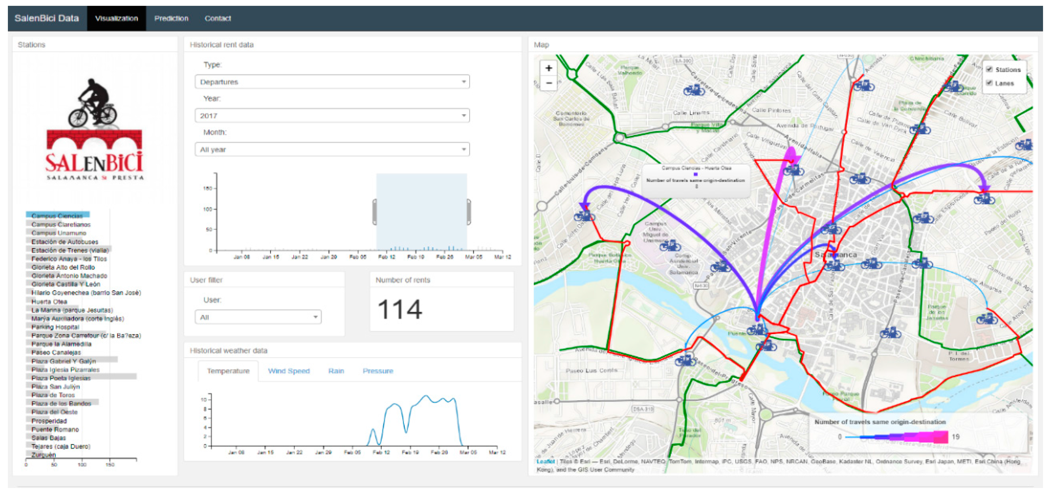
The WebAPI agent offers an API REST for third party applications which can obtain the data processed in the MAS and ask for demand predictions of the stations in the system. In addition, there is a web application where users can make visualization and prediction tasks. The web application consists of two sections; in Figure 16 we can see an initial view of the visualization section. In this section, it is possible to view the trips travelled in the system by year and month.
The visualization feature has various sections where data can be looked up by introducing a particular station, time (year, month and day), trip (arrivals or departures) and user. These sections act as filters and thus allow to visualize a series of specific data. In Figure 17, we can see the map with departures from the selected station, within the time period indicated in the left corner of the image. The number of trips at the selected station is represented by an arrow, its colour scale and width is proportional to the number of rides made between the station of origin and the destination.
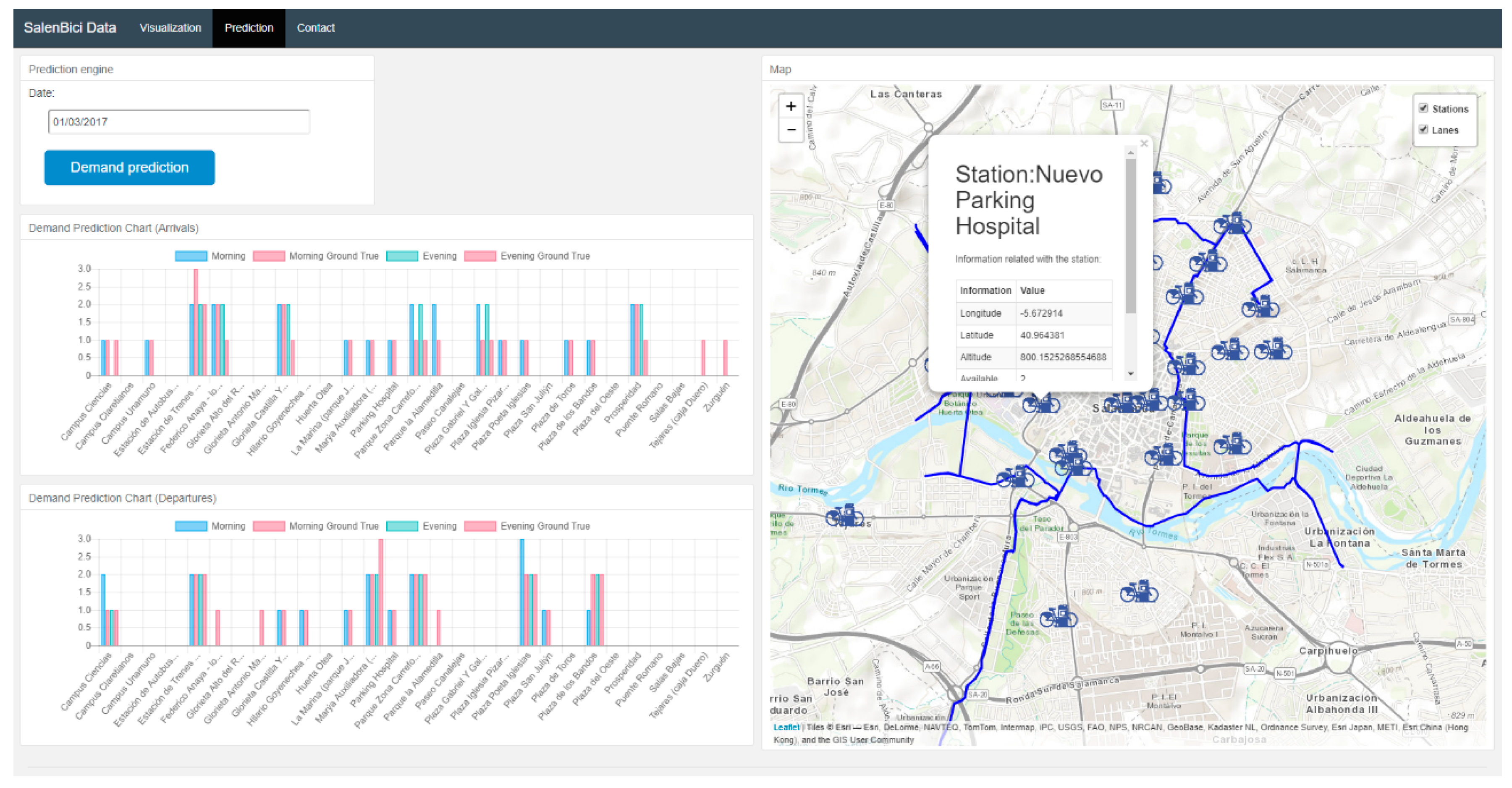
Trips between the station of origin and the rest of stations are represented with arrows, whose colour and width is proportional to the number of rides made between a particular station and the rest. These visualizations allow the BSS administrator to analyse the history of the system and find the stations with the greatest numbers of arrivals and departures. Figure 18 shows the demand prediction section which employs the selected models to predict demand at each station.
It is possible to select both, an arrow from the past and an arrow for the future. An arrow from the past, apart of showing the data collected by the system, will also visualize the prediction made by the model and the real data that were collected for that station, within the indicated date. These data will be useful to BSS administrators at the time of relocating the bicycles at the stations.
5. Conclusions and Future Works
This work proposed a multi agent system for bike sharing systems. As part of this work, a case study was conducted to test the feasibility of the system, using the data of a BSS located in Salamanca, a middle-sized city. The inclusion of agents in charge of collecting data from heterogeneous sources as well as its cleaning and fusion has eased these tasks. This agent architecture will also make it easier to obtain data from different bike sharing systems.
Moreover, the information collected by the other system agents was employed by the agents that perform demand forecasting. The use of these agents has allowed us to offer services to third party applications.
Different regression algorithms have also been employed in the process of bike demand prediction. Additionally, a statistical analysis has been performed in order to show the differences in their performance and to determine the relevance of results. Random Forest Regressor is the regressor algorithm that outperformed the rest of the algorithms.
With regards to the visualization of the data collected by the agents, a web application has been developed where it is possible to analyse and filter the previously processed data. Thanks to filters in this application the BSS operator can view the desired information thanks and have an insight on the behaviour of the users in the system.
This web application includes a prediction module where the BSS operator can request predictions for future days and make decisions in matters of bike reallocation strategies.
In future works we will employ this multi agent system to collect, process and analyse the data of BSSs in bigger cities such as Madrid.
We will also evaluate the different prediction models with that data in order to compare the performance of the system in middle-sized and big cities. Furthermore, in order to employ the output demand prediction of this system, future work will concern reallocation bike strategies in BSS and the obtaining of an optimal route.
In future works we will analyse how to include the new dock-less bike sharing systems into the developed multi agent system. We will analyse the new additional data that these kinds of systems provide and how to include them into our system. In dock-less systems, the deployed fleet of bicycles could be grouped, creating clusters which act as virtual stations in the city. This data could be used to analyse the bicycle demand and flow of dock-less bike sharing systems.
Acknowledgments
Álvaro Lozano is supported by the pre-doctoral fellowship from the University of Salamanca and Banco Santander. This work was supported by the Spanish Ministry, Ministerio de Economía y Competitividad and FEDER funds. Project. SURF: Intelligent System for integrated and sustainable management of urban fleets TIN2015-65515-C4-3-R. We would also like to show our gratitude to the SalenBici bike share system for sharing with us the data for the current work.
Author Contributions
Álvaro Lozano and Juan F. De Paz conceived and designed the multi agent system while Daniel H. De La Iglesia and Gabriel Villarrubia González contributed to the development and implementation of the system; Álvaro Lozano carried out the experimentation, the model selection and implementation and wrote the paper. Javier Bajo reviewed and supervised the whole work and provided his great expertise in the field.
Conflicts of Interest
The authors declare no conflict of interest.
References
- Pucher, J.; Buehler, R. Cycling towards a more sustainable transport future. Transp. Rev. 2017, 1–6. [Google Scholar] [CrossRef]
- Mátrai, T.; Tóth, J. Comparative assessment of public bike sharing systems. Transp. Res. Procedia 2016, 14, 2344–2351. [Google Scholar] [CrossRef]
- Midgley, P. Bicycle-sharing schemes: Enhancing sustainable mobility in urban areas. Commun. Sustain. Dev. 2011, 18, 1–12. [Google Scholar]
- European Commission—PRESS RELEASES—Press Release—Energy Union and Climate Action: Driving Europe’s Transition to a Low-Carbon Economy. Available online: http://europa.eu/rapid/press-release_IP-16-2545_en.htm (accessed on 28 June 2017).
- Plan B Updates—112: Bike-Sharing Programs Hit the Streets in over 500 Cities Worldwide|EPI. Available online: http://www.earth-policy.org/plan_b_updates/2013/update112 (accessed on 28 June 2017).
- Ricci, M. Bike sharing: A review of evidence on impacts and processes of implementation and operation. Res. Transp. Bus. Manag. 2015, 15, 28–38. [Google Scholar] [CrossRef]
- The Bike-Sharing World Map. Available online: https://www.google.com/maps/d/u/0/viewer?ll=-3.81666561775622e-14%2C-42.25341696875&spn=143.80149%2C154.6875&hl=en&msa=0&z=1&source=embed&ie=UTF8&om=1&mid=1UxYw9YrwT_R3SGsktJU3D-2GpMU (accessed on 28 June 2017).
- Dhingra, C.; Kodukula, S. Public Bicycle Schemes: Applying the Concept in Developing Cities. 2010. Available online: http://sutp.org/files/contents/documents/resources/B_Technical-Documents/GIZ_SUTP_TD3_Public-Bicycle-Schemes_EN.pdf (accessed on 15 December 2017).
- Shaheen, S.A.; Guzman, S.; Zhang, H. Bikesharing in Europe, the Americas, and Asia Past, Present, and Future. Transp. Res. Rec. J. Transp. Res. Board 2010, 2143, 159–167. [Google Scholar] [CrossRef]
- Station-Free Bike Sharing|ofo. Available online: https://www.ofo.com/us/en (accessed on 29 December 2017).
- The World’s First & Amp; Largest Smart Bike Share|Mobike. Available online: https://mobike.com/global/ (accessed on 29 December 2017).
- Share Bike Bubble Claims First Big Casualty as Bluegogo Reportedly Goes Bankrupt. Available online: http://www.smh.com.au/world/share-bike-bubble-claims-first-big-casualty-as-bluegogo-reportedly-goes-bankrupt-20171116-gzn0k9.html (accessed on 29 December 2017).
- Raviv, T.; Tzur, M.; Forma, I.A. Static repositioning in a bike-sharing system: Models and solution approaches. EURO J. Transp. Logist. 2013, 2, 187–229. [Google Scholar] [CrossRef]
- Di Gaspero, L.; Rendl, A.; Urli, T. Balancing bike sharing systems with constraint programming. Constraints 2016, 21, 318–348. [Google Scholar] [CrossRef]
- Vogel, P.; Greiser, T.; Mattfeld, D.C. Understanding bike-sharing systems using Data Mining: Exploring activity patterns. Procedia Soc. Behav. Sci. 2011, 20, 514–523. [Google Scholar] [CrossRef]
- Froehlich, J.; Neumann, J.; Oliver, N. Measuring the pulse of the city through shared bicycle programs. In Proceedings of the UrbanSense08, Raleigh, NC, USA, 4 November 2008; pp. 16–21. [Google Scholar]
- Kaltenbrunner, A.; Meza, R.; Grivolla, J.; Codina, J.; Banchs, R. Urban cycles and mobility patterns: Exploring and predicting trends in a bicycle-based public transport system. Pervasive Mob. Comput. 2010, 6, 455–466. [Google Scholar] [CrossRef]
- Kaggle INC Bike Sharing Demand|Kaggle. Available online: https://www.kaggle.com/c/bike-sharing-demand (accessed on 27 July 2017).
- Capital Bikeshare Capital Bikeshare: Metro DC’s Bikeshare Service|Capital Bikeshare. Available online: https://www.capitalbikeshare.com/ (accessed on 27 July 2017).
- Giot, R.; Cherrier, R. Predicting bikeshare system usage up to one day ahead. IEEE Symp. Ser. Comput. Intell. 2014, 1–8. [Google Scholar] [CrossRef]
- Patil, A.; Musale, K.; Rao, B.P. Bike share demand prediction using RandomForests. IJISET Int. J. Innov. Sci. Eng. Technol. 2015, 2. Available online: http://ijiset.com/vol2/v2s4/IJISET_V2_I4_195.pdf (accessed on 15 December 2017).
- Wang, W.; Wang, W.; Curley, A. Forecasting Bike Rental Demand Using New York Citi Bike Data. Master’s Thesis, Dublin Institute of Technology, Dublin, Ireland, 2016. [Google Scholar]
- Lee, C.; Wang, D.; Wong, A. Forecasting Utilization in City Bike-Share Program (Vol. 254). Technical Report, CS 229 2014 Project. 2014. Available online: http://cs229.stanford.edu/proj2014/Christina%20Lee,%20David%20Wang,%20Adeline%20Wong,%20Forecasting%20Utilization%20in%20City%20Bike-Share%20Program.pdf (accessed on 15 December 2017).
- Du, J.; He, R.; Zhechev, Z. Forecasting Bike Rental Demand. 2014. Available online: http://cs229.stanford.edu/proj2014/Jimmy%20Du,%20Rolland%20He,%20Zhivko%20Zhechev,%20Forecasting%20Bike%20Rental%20Demand.pdf (accessed on 15 December 2017).
- Yin, Y.-C.; Lee, C.-S.; Wong, Y.-P. Demand Prediction of Bicycle Sharing Systems. 2012. Available online: http://cs229.stanford.edu/proj2014/Yu-chun%20Yin,%20Chi-Shuen%20Lee,%20Yu-Po%20Wong,%20Demand%20Prediction%20of%20Bicycle%20Sharing%20Systems.pdf (accessed on 15 December 2017).
- NYC. Citi Bike Station Map. Available online: https://member.citibikenyc.com/map/ (accessed on 27 July 2017).
- Lluís Esquerda CityBikes: Bike Sharing Networks around the World. Available online: https://citybik.es/ (accessed on 27 July 2017).
- SalEnBici Salenbici. Sistema de Préstamo de Bicicletas de Salamanca. Salenbici. Available online: http://www.salamancasalenbici.com/ (accessed on 27 July 2017).
- Matos, D.M.; Lopes, B.; Bento Dei, C.; Machado, E.R. An Intelligent Bike-Sharing Rebalancing System; Universidade de Coimbra: Coimbra, Portugal, 2015. [Google Scholar]
- Chicago Bike Share System Divvy: Chicago’s Bike Share Program|Divvy Bikes. Available online: https://www.divvybikes.com/ (accessed on 27 July 2017).
- Capital Bike Share Whasington System Data|Capital Bikeshare. Available online: https://www.capitalbikeshare.com/system-data (accessed on 27 July 2017).
- Billhardt, H.; Fernandez, A.; Lujak, M.; Ossowski, S.; Julian, V.; De Paz, J.F.; Hernandez, J.Z. Coordinating open fleets. A taxi assignment example. AI Commun. 2017, 30, 37–52. [Google Scholar] [CrossRef]
- Gregori, M.E.; Cámara, J.P.; Bada, G.A. A jabber-based multi-agent system platform. In Proceedings of the Fifth International Joint Conference on Autonomous Agents and Multiagent Systems—AAMAS ‘06, Hakodate, Japan, 8–12 May 2006; ACM Press: New York, NY, USA, 2006; p. 1282. [Google Scholar]
- Criado, N.; Argente, E.; Julian, V.; Botti, V. Organizational services for the spade agent platform. IEEE Lat. Am. Trans. 2008, 6, 550–555. [Google Scholar] [CrossRef]
- Bellifemine, F.; Poggi, A.; Rimassa, G. JADE—A FIPA-compliant agent framework. Proc. PAAM 1999, 99, 33. [Google Scholar]
- Zato, C.; Villarrubia, G.; Sánchez, A.; Barri, I.; Rubión, E.; Fernández, A.; Rebate, C.; Cabo, J.A.; Álamos, T.; Sanz, J.; et al. PANGEA—Platform for Automatic Construction of Organizations of Intelligent Agents; Springer: Berlin/Heidelberg, Germany, 2012; pp. 229–239. [Google Scholar]
- Villarrubia, G.; Paz, J.F.; De Iglesia, D.H.D.; La Bajo, J. Combining multi-agent systems and wireless sensor networks for monitoring crop irrigation. Sensors 2017, 17, 1775. [Google Scholar] [CrossRef] [PubMed]
- Aiomas—Aiomas 1.0.3 Documentation. Available online: http://aiomas.readthedocs.io/en/latest/ (accessed on 14 November 2017).
- osBrain—0.5.0—osBrain 0.5.0 Documentation. Available online: http://osbrain.readthedocs.io/en/stable/ (accessed on 14 November 2017).
- Esquerda, L. Documentation|CityBikes API. Available online: https://api.citybik.es/v2/ (accessed on 4 October 2017).
- Citi Bike System Data|Citi Bike NYC. Available online: https://www.citibikenyc.com/system-data (accessed on 4 October 2017).
- Weather Forecast & Amp; Reports—Long Range & Amp; Local|Wunderground|Weather Underground. Available online: https://www.wunderground.com/ (accessed on 4 October 2017).
- Agencia Estatal de Meteorología—AEMET. Gobierno de España; AEMET: Madrid, Spain, 2017.
- Workalendar. Available online: https://github.com/novafloss/workalendar (accessed on 5 October 2017).
- Pedregosa Fabianpedregosa, F.; Alexandre Gramfort, N.; Michel, V.; Thirion Bertrandthirion, B.; Grisel, O.; Blondel, M.; Prettenhofer Peterprettenhofer, P.; Weiss, R.; Dubourg, V.; Vanderplas Vanderplas, J.; et al. Scikit-learn: Machine Learning in Python Gaël Varoquaux. J. Mach. Learn. Res. 2011, 12, 2825–2830. [Google Scholar]
- Breiman, L. Random Forests. Mach. Learn. 2001, 45, 5–32. [Google Scholar] [CrossRef]
- Friedman, J.H.; Friedman, J.H. Greedy function approximation: A gradient boosting machine. Ann. Stat. 2000, 29, 1189–1232. [Google Scholar] [CrossRef]
- Regue, R.; Recker, W. Using gradient boosting machines to predict bikesharing station states. In Proceedings of the 93rd Annual Meeting of Transportation Research Board, Washington, DC, USA, 12–16 January 2014. [Google Scholar]
- Malani, J.; Sinha, N.; Prasad, N.; Lokesh, V. Forecasting Bike Sharing Demand. Available online: https://cseweb.ucsd.edu/classes/wi17/cse258-a/reports/a050.pdf (accessed on 15 December 2017).
- Prakash Nekkanti, O. Prediction of Rental Demand for a Bike-Share Program. 2017. Available online: https://library.ndsu.edu/ir/handle/10365/25949 (accessed on 15 December 2017).
- Kang, S.C.; Otani, T.W. Learning to Predict Demand in a Transport-Resource Sharing Task; Naval Postgraduate School: Monterey, CA, USA, 2015. [Google Scholar]
- Grupo Bimbo Inventory Demand|Kaggle. Available online: https://www.kaggle.com/c/grupo-bimbo-inventory-demand (accessed on 15 November 2017).
- Sberbank Russian Housing Market|Kaggle. Available online: https://www.kaggle.com/c/sberbank-russian-housing-market (accessed on 15 November 2017).
Figure 1.
One of BiciMad System’s bike docking stations (Madrid, Spain) with electrical bikes.
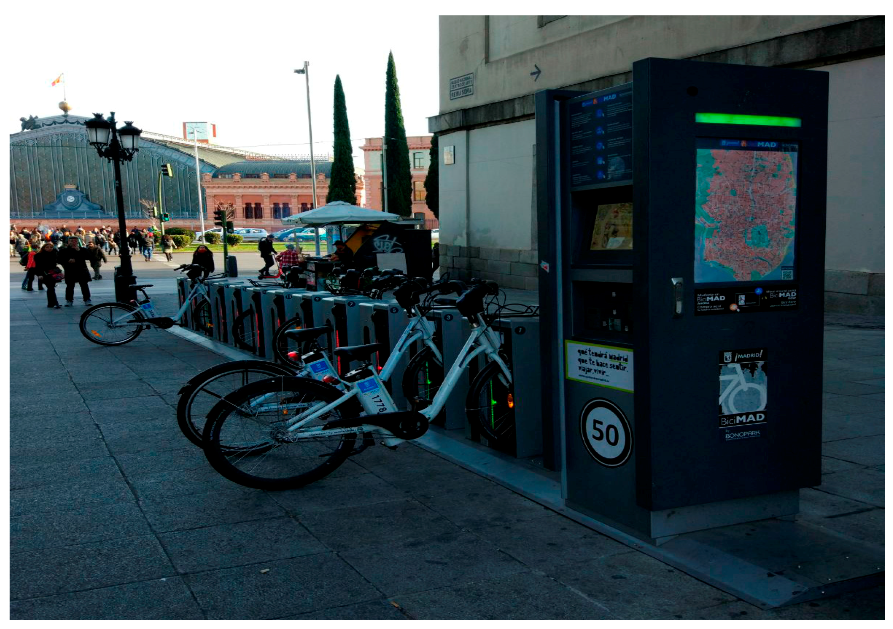
Figure 2.
General diagram of the proposed multi agent system for bike sharing systems.

Figure 3.
Data processing flow chart of the processes performed by the data processor agent.
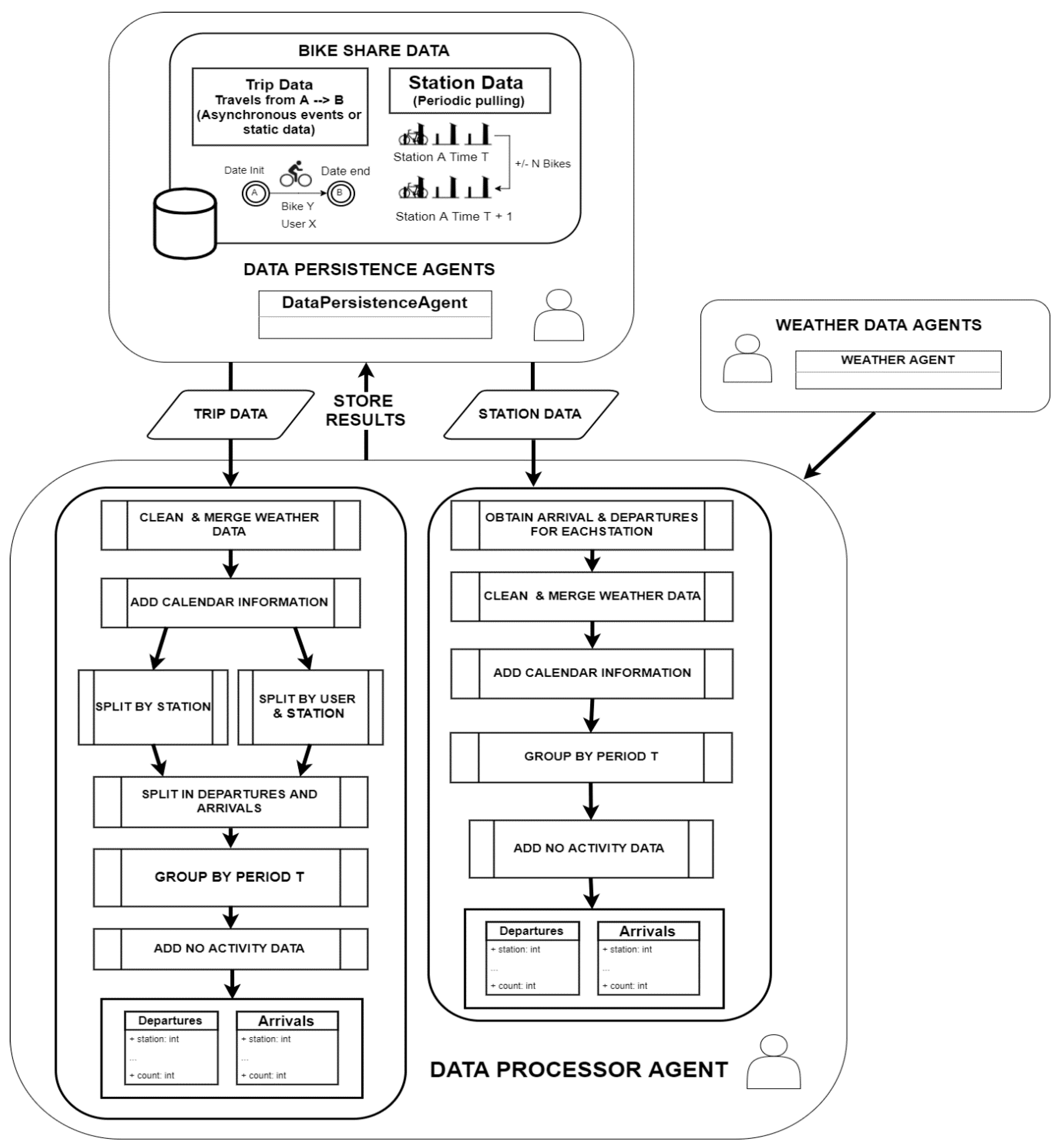
Figure 4.
(a) One of the trucks of the SalenBici system operators; (b) Map of the stations provided by the council of Salamanca.
Figure 4.
(a) One of the trucks of the SalenBici system operators; (b) Map of the stations provided by the council of Salamanca.
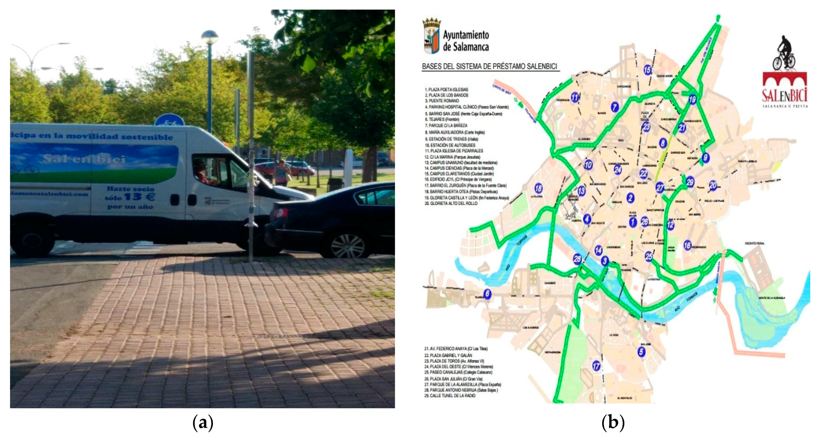
Figure 5.
Sequence diagram of trip data loading by multiagent system.

Figure 6.
Total number of events (arrivals or departures) performed in Bike sharing systems (BSS) SalenBici from January 2013 until March 2017.
Figure 6.
Total number of events (arrivals or departures) performed in Bike sharing systems (BSS) SalenBici from January 2013 until March 2017.

Figure 7.
Periods of working time of each station in the BSS SalenBici.

Figure 8.
Data splitting for model training and selection.

Figure 9.
Root Mean Square Logarithmic Error (RMSLE) provided by each algorithm for each station in the arrivals data.
Figure 9.
Root Mean Square Logarithmic Error (RMSLE) provided by each algorithm for each station in the arrivals data.
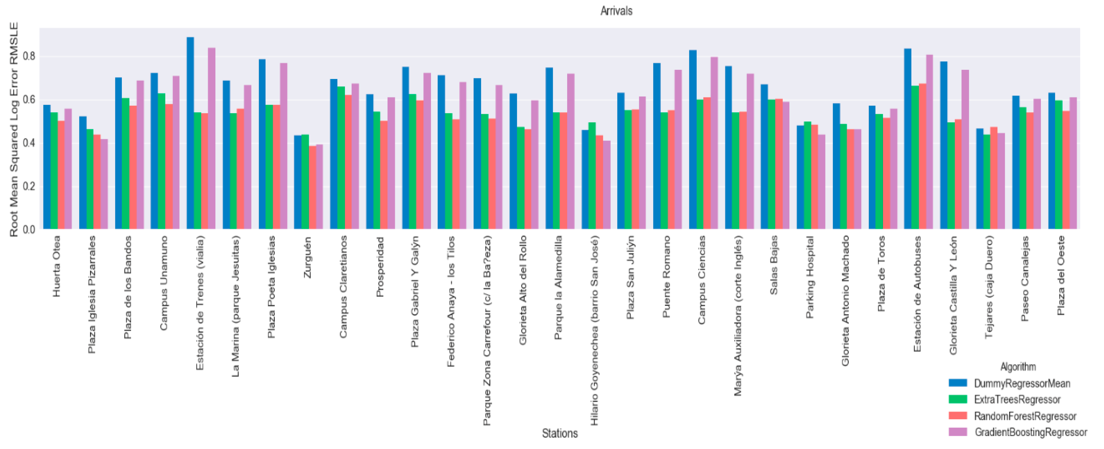
Figure 10.
RMSLE provided by each algorithm for each station in the departures data.
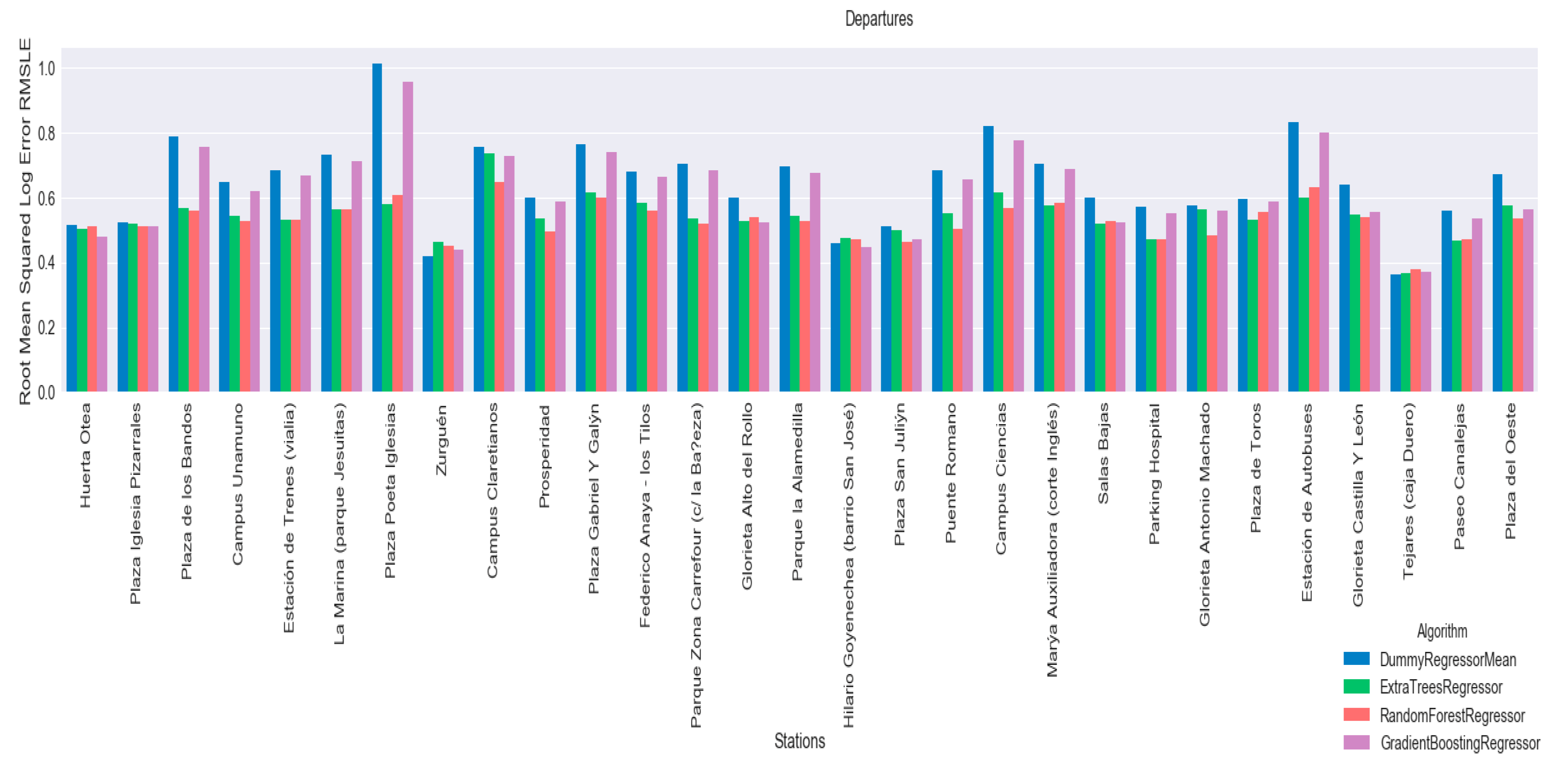
Figure 11.
Coefficient of determination of models for the arrivals at each station.

Figure 12.
Coefficient of determination of models for departures from each station.

Figure 13.
Mann-Whitney U test two sided for (a) arrivals and (b) departures.
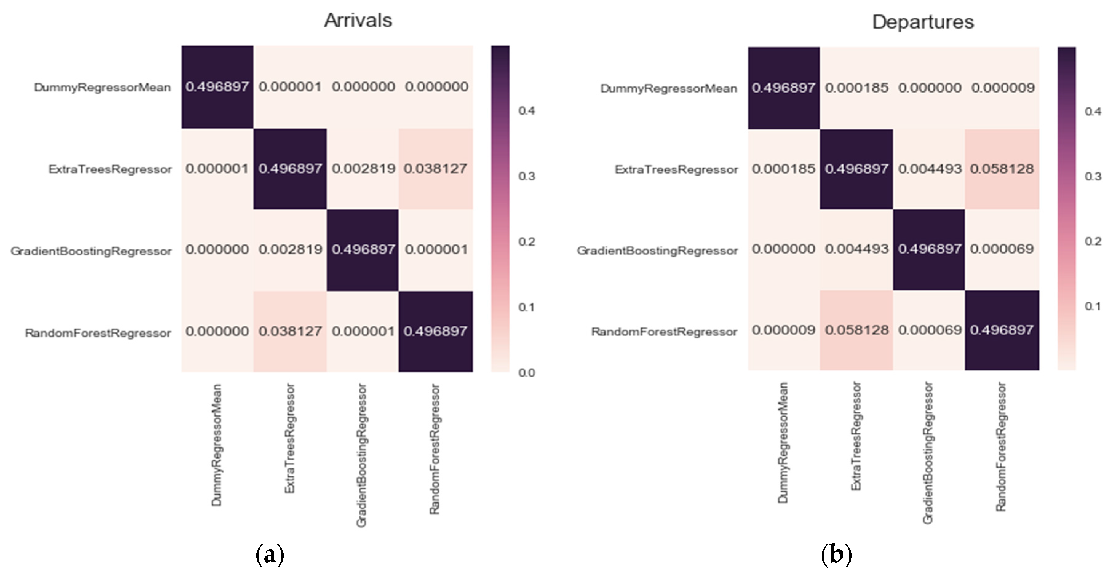
Figure 14.
Mann-Whitney U test greater for (a) arrivals and (b) departures.
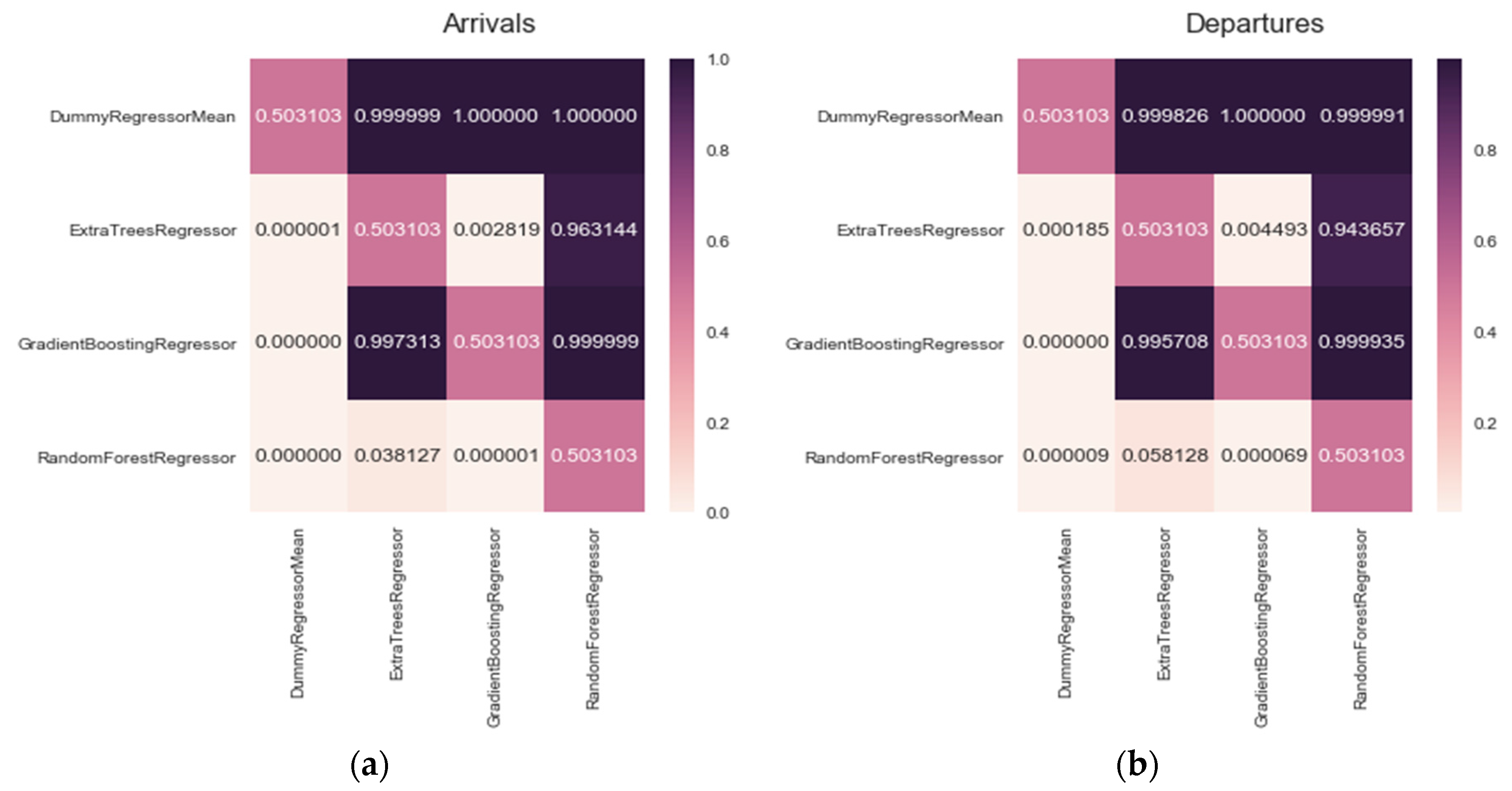
Figure 15.
Sequence diagram of trip data loading by multiagent system.

Figure 16.
Web application served by the WebAPI agent. Visualization of the historical data section.
Figure 16.
Web application served by the WebAPI agent. Visualization of the historical data section.
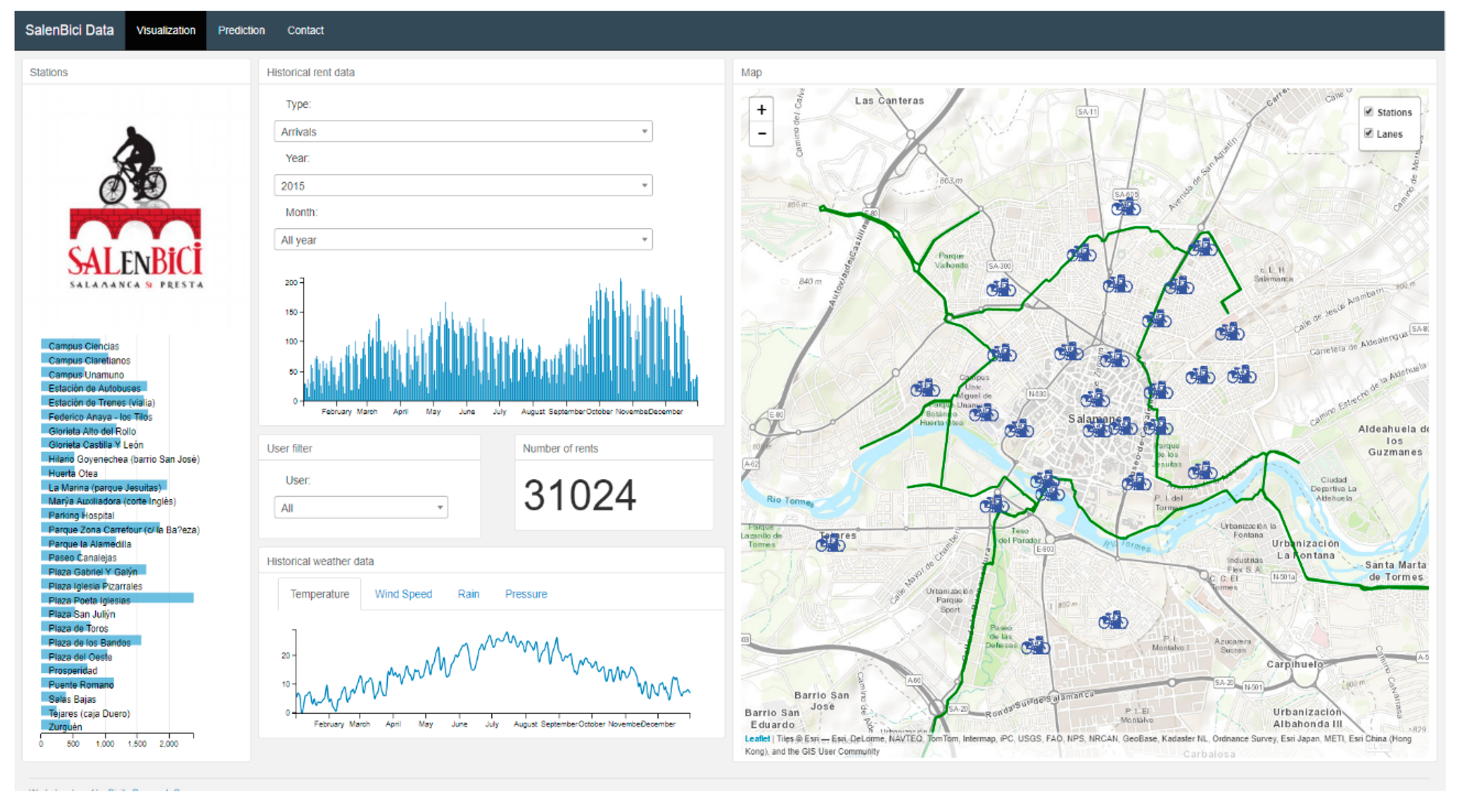
Figure 17.
Visualization section. Where a station is selected for a period of time and the number of trips (origin-destination) is visualized.
Figure 17.
Visualization section. Where a station is selected for a period of time and the number of trips (origin-destination) is visualized.

Figure 18.
Prediction tool section.
© 2018 by the authors. Licensee MDPI, Basel, Switzerland. This article is an open access article distributed under the terms and conditions of the Creative Commons Attribution (CC BY) license (http://creativecommons.org/licenses/by/4.0/).
Share and Cite
MDPI and ACS Style
Lozano, Á.; De Paz, J.F.; Villarrubia González, G.; Iglesia, D.H.D.L.; Bajo, J. Multi-Agent System for Demand Prediction and Trip Visualization in Bike Sharing Systems. Appl. Sci. 2018, 8, 67. https://doi.org/10.3390/app8010067
AMA Style
Lozano Á, De Paz JF, Villarrubia González G, Iglesia DHDL, Bajo J. Multi-Agent System for Demand Prediction and Trip Visualization in Bike Sharing Systems. Applied Sciences. 2018; 8(1):67. https://doi.org/10.3390/app8010067
Chicago/Turabian StyleLozano, Álvaro, Juan F. De Paz, Gabriel Villarrubia González, Daniel H. De La Iglesia, and Javier Bajo. 2018. "Multi-Agent System for Demand Prediction and Trip Visualization in Bike Sharing Systems" Applied Sciences 8, no. 1: 67. https://doi.org/10.3390/app8010067
Note that from the first issue of 2016, this journal uses article numbers instead of page numbers. See further details here.