A Method to Decompose the Streamed Acoustic Emission Signals for Detecting Embedded Fatigue Crack Signals


1
Civil and Materials Engineering, University of Illinois at Chicago, Chicago, IL 60607, USA
2
Mechanical and Industrial Engineering, University of Illinois at Chicago, Chicago, IL 60607, USA
3
NAVAIR NAS Patuxent River, St. Mary’s County, MD 20670, USA
*
Author to whom correspondence should be addressed.
Appl. Sci. 2018, 8(1), 7; https://doi.org/10.3390/app8010007
Submission received: 12 November 2017
/
Revised: 13 December 2017
/
Accepted: 19 December 2017
/
Published: 22 December 2017
(This article belongs to the Section Acoustics and Vibrations)
Abstract
:The data collection of Acoustic Emission (AE) method is typically based on threshold-dependent approach, where the AE system acquires data when the output of AE sensor is above the pre-defined threshold. However, this approach fails to detect flaws in noisy environment, as the signal level of noise may overcome the signal level of AE from flaws, and saturate the AE system. Time-dependent approach is based on streaming waveforms and extracting features at every pre-defined time interval. It is hypothesized that the relevant AE signals representing active flaws are embedded into the streamed signals. In this study, a decomposition method of the streamed AE signals to separate noise signal and crack signal is demonstrated. The AE signals representing fatigue crack growth in steel are obtained from the laboratory scale testing. The streamed AE signals in a noisy operational condition are obtained from the gearbox testing at the Naval Air Systems Command (NAVAIR) facility. The signal addition and decomposition is achieved to determine the minimum detectable signal to noise ratio that is embedded into the streamed AE signals. The developed decomposition approach is demonstrated on detecting burst signals embedded into the streamed signals recorded in the spline testing of the helicopter gearbox test rig located at the NAVAIR facility.

1. Introduction
The spline structure of helicopter gearbox is prone to develop cracks and spalling due to excessive loads, insufficient lubricants, manufacturing defects, installation problems, or material fatigue. The common nondestructive evaluation (NDE) methods to monitor flaws in splines are debris monitoring, acoustic emission, and vibration. The methods can be applied individually [1,2,3,4,5,6] or concurrently [7,8]. While debris monitoring does not require any electronics, it is simple to interpret and has excellent sensitivity to wear-related failure; this method is insufficient to non-benign cracks as no debris is produced. Acoustic emission (AE) and vibration signals have more quantitative results to detect the earliest stage of damage in rotating machinery.
AE and vibration methods are based on recording transient signals in two different frequency spectrums. While vibration method is based on features that are extracted from time and frequency domain signals recorded by low frequency accelerometers in order to assess the changes in vibrational properties as related to the damage [9,10], AE method is based on detecting propagating elastic waves released from active flaws. While the AE source in metals has broad spectrum of up to 1 MHz [11], and typical frequency range is 60–300 kHz to overcome the challenge of signal attenuation in higher frequencies and increase the distance between source and sensor. The common sources that generate AE in gearbox include plastic deformation, microfracture, wear, bubbles, friction and impact [12]. Once transient signals are collected, signal processing methods, such as wavelet decomposition [13], empirical mode decomposition [6], and multivariate pattern recognition [14] are applied. Typical parameters extracted from the transient signals are root mean square value, frequency domain characteristics, energy, spectral kurtosis, and peak-to-peak vibration level. Due to the difference in the frequency bandwidth, AE method is more sensitive to micro cracks as compared to the vibration method.
Typical AE data acquisition approach is based on threshold: an AE signal is detected when the signal level is above threshold. This approach may cause high hit-rate for noisy applications, such as gearbox monitoring. Another approach is to collect long duration waveforms (100–200 ms) with high sampling rate (1–2 MHz) at every time interval (2–5 s), and analyze the waveforms in post-processing. As crack growth is a stochastic process, it is considered that while some data will be lost due to the idle time of data acquisition system between waveform recording intervals, crack information will be stochastically detected. However, it is important to identify how to analyze long duration signals in order to reduce the influence of background noise from the extracted features. In this study, the streamed AE signals are recorded from the helicopter gearbox test rig at the Naval Air Systems Command (NAVAIR) facility. The AE signature of the fatigue crack growth is obtained from the scaled laboratory experiments. The spline section of the gearbox is modeled as a planar geometry, such that the crack growth direction is similar to the expected crack growth in a realistic condition. The streamed AE signal and the crack AE signal are merged with different signal to noise ratios in order to determine the minimum detectable AE signal amplitude due to the crack growth as compared to the background noise level; therein, the streamed signals are selected within the acoustically stable regions and in the early stage of testing as no crack is expected. A decomposition approach of the streamed AE signal to extract the crack information is developed. Additionally, the developed methodology is demonstrated on detecting burst signals that are embedded into the streamed signals recorded in the spline testing of the helicopter gearbox test rig located at the NAVAIR facility.
The organization of this paper is as follows. Section 2 describes the experimental designs at the NAVAIR facility and the laboratory. The experimental results are presented in Section 3. Section 4 presents the signal processing method of the integration of the stream and crack growth signals, and the application of identification of burst signals in the NAVAIR test rig. The discussion and conclusions of this study are presented in Section 5.
2. Description of Experiments
2.1. Description of Gearbox Testing (NAVAIR Gearbox Test)
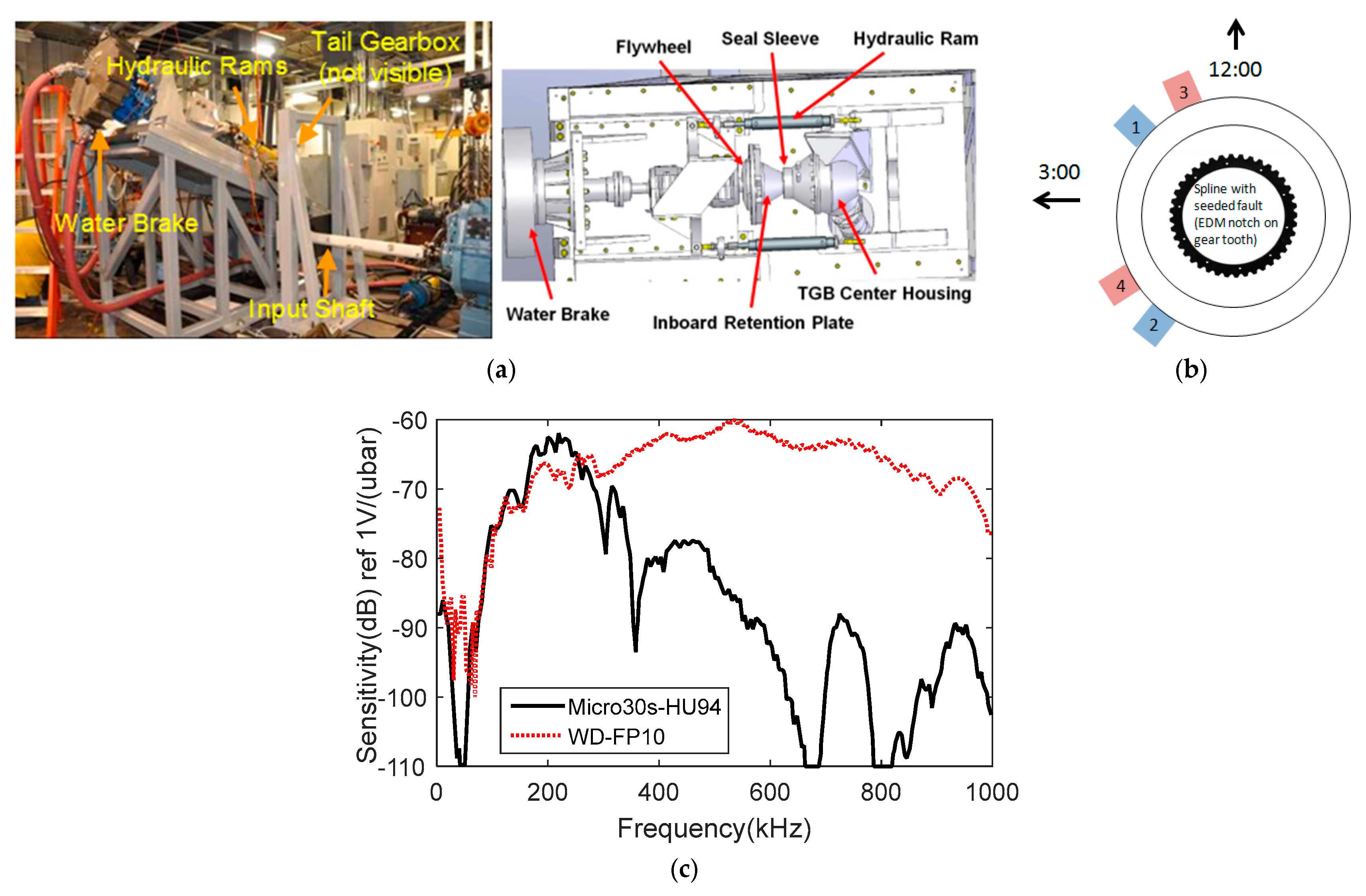
NAVAIR-4.4.2 has built an experimental test stand to replicate the failure progression under complex loading and determine the ideal NDE strategies. Figure 1a shows the test stand and the mechanical details. The 2.5 h block cycle in the controlled environment simulates 2.5 flight hours in an average mission. EMD (Electrical discharge machining) notch is introduced to control the crack growth location. The test rig can produce the multilevel block cycle with torque, trust, and bending moment. The hub moment is identified as the primary driver of crack growth and creates one per revolution cyclic stress in the spline gear; and also, the direction of hub moment is changed for simulating different flight scenarios. The bench test includes standard strain sensors, proximity probes, thermocouples, accelerometers, and load sensors, in addition to the AE sensors. The AE data acquisition and sensing system consist of PCI-2 (Peripheral Component Interconnect) data acquisition system, and two different sensor types, including WD (wideband sensor) and micro 30 sensors manufactured by Mistras Group Inc. (Princeton Junction, NJ, USA). WD sensor has wideband response spanning 100 kHz to 1 MHz; micro 30 sensor has the bandwidth of 150–400 kHz. The resonant behaviors of the AE sensors significantly influence the output signal [15]. Figure 1c shows the calibration curves of WD and micro 30 sensors. It is important to utilize the same sensors in the laboratory testing. The AE sensors are coupled using vacuum grease and the coupling state is secured with aluminum brackets. Two sensors of each type are placed at different locations on the gearbox, as shown in Figure 1b. Time-dependent approach independent from threshold is implemented to record the AE data. The streamed AE waveforms with 150 ms duration and 2 MHz sampling rate are recorded at every 5 s.
2.2. Laboratory Scale Fatigue Testing (UIC Fatigue Test)
In order to identify the AE signature due to the fatigue crack growth, a laboratory scale testing with similar characteristics as the NAVAIR testing is designed. However, some simplifications are made in defining the loading condition and sample geometry. The loading condition is fatigue causing tensile stress at the notch tip. The circular geometry of the spline section is built as a planar geometry in order to apply loading in conventional test equipment, while the other geometric details of the spline section (e.g., thickness, spline details) are preserved, as shown in Figure 2. A more comprehensive discussion of the laboratory testing is presented in [16]. Similar to the NAVAIR test rig, a notch is introduced to control the initiation of crack. To ensure that the crack direction is perpendicular to the spline tooth, the cyclic load (4 Hz, , max load = 12 kN) is applied using the load control scheme of Instron loading machine (Instron, Norwood, MA, USA). The AE monitoring system includes three WD sensors placed in a triangulation form for source localization; one Nano 30 sensor (nano-30 FP 97 sensor manufactured by Mistras Group Inc.); and, piezoelectric wafer sensor array, see in Figure 2c. The AE sensors are bonded using super glue and connected to 40 dB gain pre-amplifiers. The AE data is collected using PCI-8 data acquisition board manufactured by Mistras Group Inc. Each AE waveform is recorded with 3 MHz sampling rate with the duration of 1 ms. The threshold is varied between 50 dB and 70 dB to control the hit rate [16]. In addition, strain data is collected throughout the fatigue test to capture the strain level change due to the crack growth. The crack length reaches to 7 mm after 590,211 cycles, as shown in Figure 3. The acoustic microscope image is taken using the Sonoscan Gen 6 C-SAM acoustic microscope (Sonoscan, Inc., Elk Grove Village, IL, USA) and 100 MHz transducer with 60 μm resolution.
2.3. Similarity and Differences of The NAVAIR Test Rig and The Laboratory Testing
The purpose of the UIC laboratory experiments is to simulate fatigue crack growth other than simulating fretting noise. The burst type AE signals due to the crack growth of the UIC fatigue test is embedded into the streamed AE signals that were obtained from the NAVAIR gearbox test to understand the detectability of crack signal from the streamed AE signals. The purpose is to identify the operational noise signal from the NAVAIR gearbox test and the crack AE signal from the UIC fatigue test for developing an efficient signal processing method to extract the crack signal from the streamed waveforms. Therefore, it is important to identify if two test conditions are comparable.
The comparison of the NAVAIR gearbox test and the UIC fatigue test is summarized in Table 1. The AE sensor types and spline geometry of both experiments are similar. The motion of spline gear in the helicopter is rotation, and the fatigue crack initiates and grows after certain numbers of rotational loading. The direction of crack growth is typically perpendicular to the spline based on the NAVAIR statistical data.
The crack directions from the NAVAIR test rig and the UIC fatigue test are compared in Figure 3. The crack generated in the actual spline is in the circumferential direction of splines similar to the crack growth pattern of the planar geometry. For the driving loads of crack, there are two types of loaded splines in rotorcraft that experience fretting that would lead to either wear or crack initiation. The first loading condition is more common in drive shafts, and there is little moment that is applied to drive shafts that can produce a crack that grows normal to the axis of the shaft. This condition generally produces wear that erodes the spline until all of the splines are too thin to transfer the torque at which point overload occurs. The second loading condition occurs when the splines are in tension from the preload, and the gyroscopic loads are very high and cause a reverse bending situation. This condition causes the crack initiated by spline fretting to grow perpendicular to the shaft axis.
3. Experimental Results
Waveform Characteristics
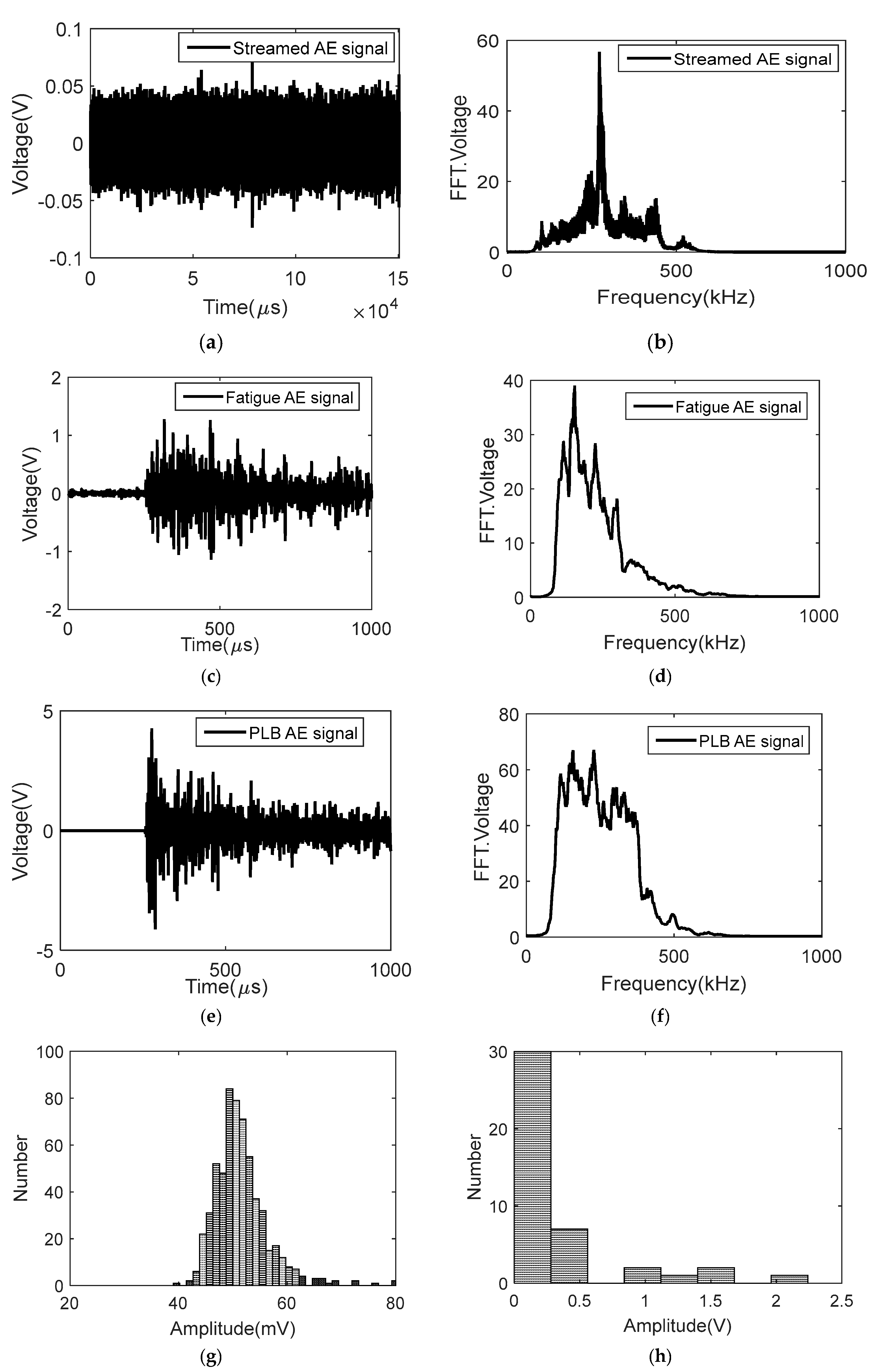
The streamed AE signals are selected from the NAVAIR gearbox test in the early stage of testing, as no crack is expected to occur and within the acoustically stable regions of testing right after the shaft rotation reaches to its full speed. The AE signals are highly influenced by the initiation and ending of gearbox operation until it reaches the stable rotational speed. The selected streamed AE signal is shown in Figure 4a,b in time domain and frequency domain, respectively. The duration of the streamed AE signal is 150 ms with the amplitude of 50 mV for the selected streamed signal. A digital filter of 20 kHz to 400 kHz is applied to the streamed waveform in order to have the same frequency range as the UIC fatigue test. The sampling frequency of the NAVAIR gearbox test is 2 MHz, while the sampling frequency of the UIC fatigue test is 3 MHz. The waveforms of the NAVAIR gearbox test is resampled in order to bring both test conditions identical.
Figure 4c,e shows the time history signals of the UIC fatigue test due to the crack growth, and the pencil lead break (PLB), respectively. The crack signal causes less energy release than the PLB signal. The peak amplitude of the crack growth is 1.292 V for the selected AE event, while it is 4.052 V due to PLB. The amplitude of the crack growth depends on the energy release caused by the crack jump. The histograms of AE amplitudes obtained from the first day of NAVAIR gearbox test and the clustered events near the notch tip of UIC fatigue test are shown in Figure 4g,h, respectively. The selected waveforms represent examples of the streamed AE signals and the fatigue crack signal. There are also slight differences in the frequency spectra of two AE sources as shown in Figure 4d,f due to the differences in source functions. The crack growth causes dipole source generated parallel to the planar direction of the specimen, while the PLB source causes monopole source that is generated at about angled with respect to the planar direction of the specimen.
On the other hand, there are some differences in the frequency spectra of the streamed AE signal and the crack AE signal. The durations of AE signals are 150 ms and 1 ms for the NAVAIR gearbox test, and the UIC fatigue test, respectively. For better understanding the characteristics of the streamed signal, a time window of 1 ms (similar to the UIC fatigue test) is defined to calculate AE power, peak frequency, and frequency centroid, as shown in Figure 5. Additionally, a windowed analysis is applied to the pre-trigger region of the crack signal in order to determine the operational noise of the UIC fatigue test, as shown in Figure 6. The environmental noise characteristics of the NAVAIR gearbox test and the UIC fatigue test have some differences, as expected; however, the peak frequencies are similar. Figure 7 shows the AE features in each time window and their distributions. In general, they have similar features and normal distribution.
The summary of the mean AE features obtained from the entire streamed signal, the windowed streamed signal in comparison to the crack signal, the noise signal of UIC fatigue test, and the PLB signal are shown in Table 2. The entire and windowed stream signals have similar characteristics. The AE power and frequency information of the crack growth signal and the streamed signal are significantly different due to the difference in the energy releases of the operational noise of the NAVAIR gearbox test and the crack signal of the UIC fatigue test.
4. The Integration of the Streamed and Crack Growth Signals
Signal is defined as the crack growth signal of the UIC fatigue test and noise is defined as the streamed AE signal of the NAVAIR gearbox test. AE signals with different signal to noise ratios (SNRs) are generated by embedding the crack signal into the streamed signal. The SNRs are obtained by calculating the square of the voltage amplitude ratio [17]:
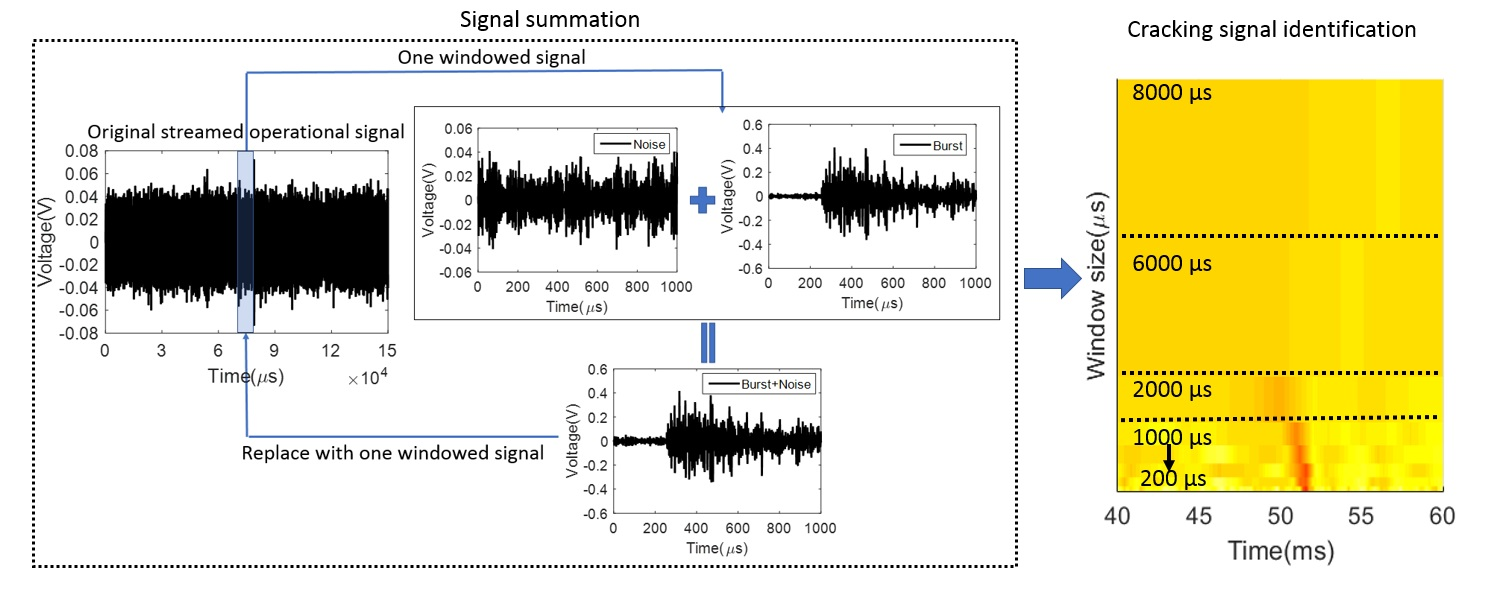
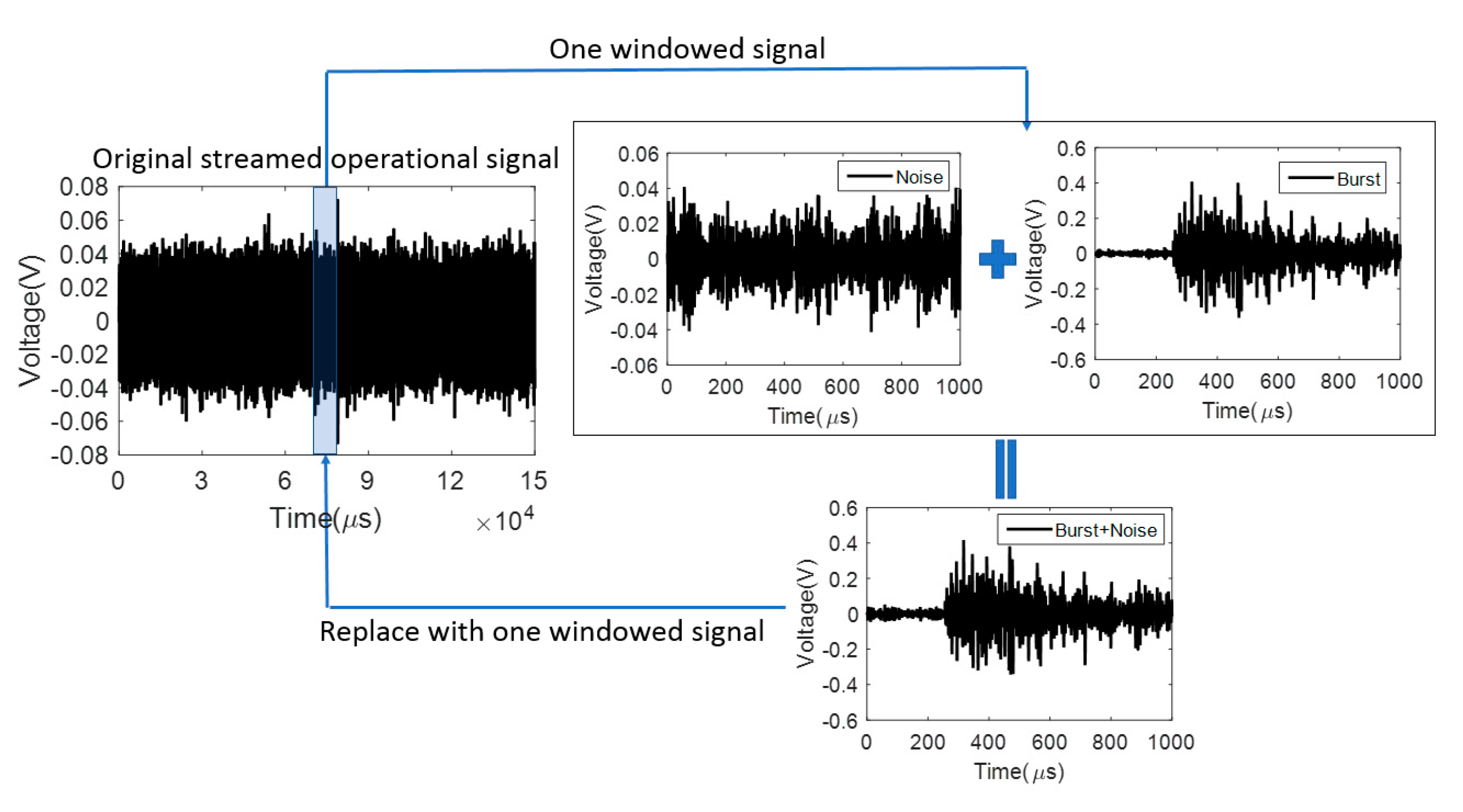
where A is the root mean square (RMS) voltage amplitude. The amplitude of the crack signal is adjusted with respect to the amplitude of the streamed signal in order to have SNRs in the range of 1.0 to 7.5. Signal amplitude, in Equation (1), represents the adjusted amplitude of the crack signal, noise amplitude , epresents the actual amplitude of the streamed signal. The methodology to combine the signals is illustrated in Figure 8 for the SNR of 7.5.
The positions of the embedded crack signal are randomly selected. A total of 150 partial signals are produced by decomposing the 150 ms long streamed signal with 1 ms window size. A random number is selected in the range of 1 to 150 using the Matlab software (MATLAB 8.5, The MathWorks, Inc, Natick, MA, USA, 2015), and the crack signal is embedded into the position of the selected random number. The streamed signals with different embedded crack signals and SNRs are compared in Figure 9. As expected from the AE features listed in Table 2, higher frequency components (>200 kHz) are dominant in the streamed signals, while the embedded crack signals influence the lower frequency components (<200 kHz). The embedded signal becomes more difficult to identify in both time and frequency domains with the decrease of SNR. It is important to note that the crack growth releases wideband signal; therefore, it is not expected to have a complete overlap of the frequency spectra of the crack signal and the background noise signal.
4.1. Signal Decomposition
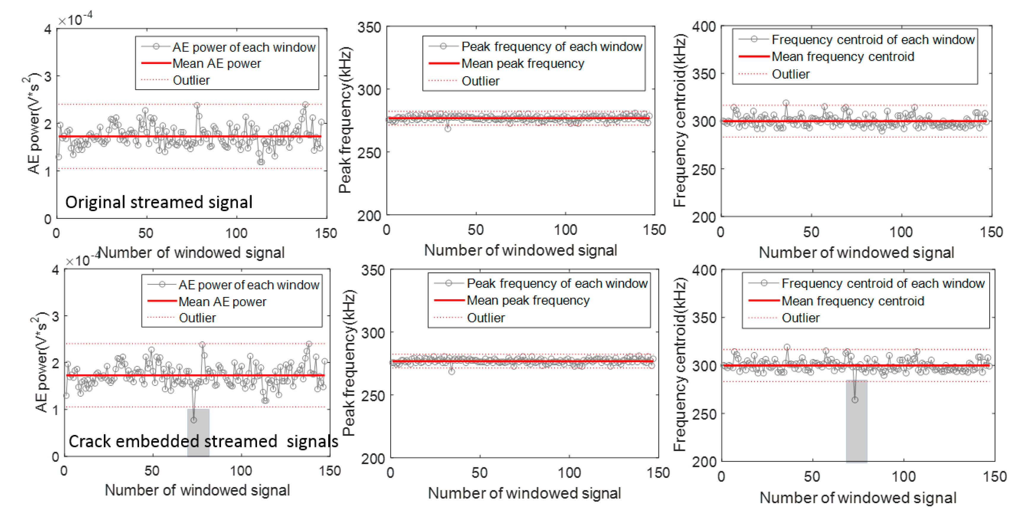
When the SNR of combined signal is equal to 1.0, the AE features are controlled by the noise signal characteristics if the AE features are extracted using the entire streamed waveform. The AE features are extracted by dividing the streamed AE signal into sections of 1 ms duration. The positions of unusual data representing AE power, peak frequency, and frequency centroid are determined by the outlier rule, according to the mean and standard deviations. The upper and lower limits are defined as , where is mean value and σ is standard deviation. The data points outside the boundary limits are defined as outliers. Two examples are shown in Figure 10 and Figure 11. The SNR is adjusted as 1.0 and the cracking signals are embedded at 74 ms and 120 ms, respectively. The data at the boundary of lower and upper bound limits present only in individual feature plots are not considered as outliers. For instance, there is a data point at the AE power plot near 140 ms, which is not present in the frequency centroid plot. The data points with the highest divergence from the mean and the limits and the present in both AE power and frequency centroid are considered to represent the presence of crack related signal. While the AE power and the frequency centroid can successfully identify the position of crack signal, the peak frequency is still influenced by the streamed signal. The decomposition of each streamed waveform into a window of typical AE signal allows for identifying the crack signal that is embedded into the background noise.
4.2. Detectable Fatigue Crack Energy with Respect to Background Noise
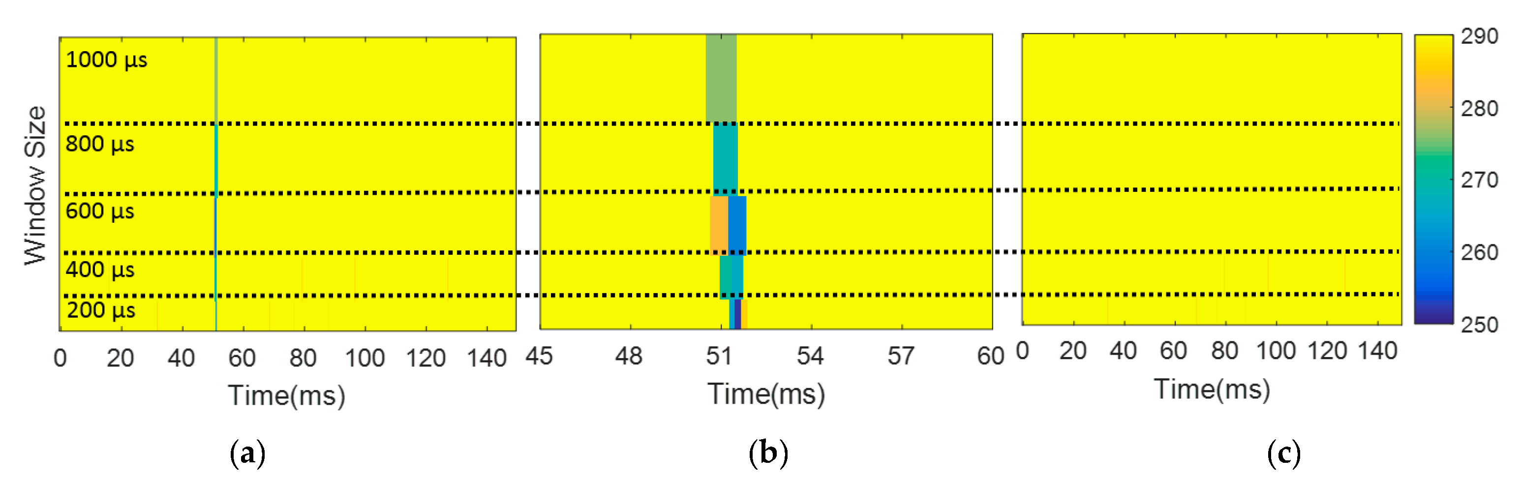
In the previous section, the decomposition of streamed signal is shown as a feasible way to identify the crack signals from the streamed signals with low SNR. However, the window size selection is an important variable to determine the position of the crack signal. Several window sizes, including 200 μs, 400 μs, 600 μs, 800 μs, and 1000 μs, are selected, and the AE feature extraction is repeated. The window size is limited to 200 μs in order to obtain good frequency resolution in the range of 20–400 kHz. The crack signal is embedded at 51 ms. Figure 12 shows the spectra of frequency centroid. The embedded crack signal can be identified clearly, as shown in Figure 12a,b by the decrease of frequency centroid in the range of 260–270 kHz near 51 s, as indicated by the color change in the spectra. The spectra of frequency centroid obtained from the original streamed signal are shown in Figure 12c, which has uniform distribution of frequency centroid throughout the streamed signal and no indication of the crack signal. Similarly, the spectra of AE power can also be used to identify the crack signal, as shown in Figure 13. However, as SNR is one, the amplitude related feature of AE power could cause artificial outlier signals, as observed near 115 s in Figure 13. If SNR is greater than one, AE power also separates the crack related activity from the secondary sources. However, the spectra of peak frequency fail to distinguish the crack signal, as seen in Figure 14. If SNR is greater than one, all three features identify the position of the embedded crack signal when the window size is less than 1 ms.
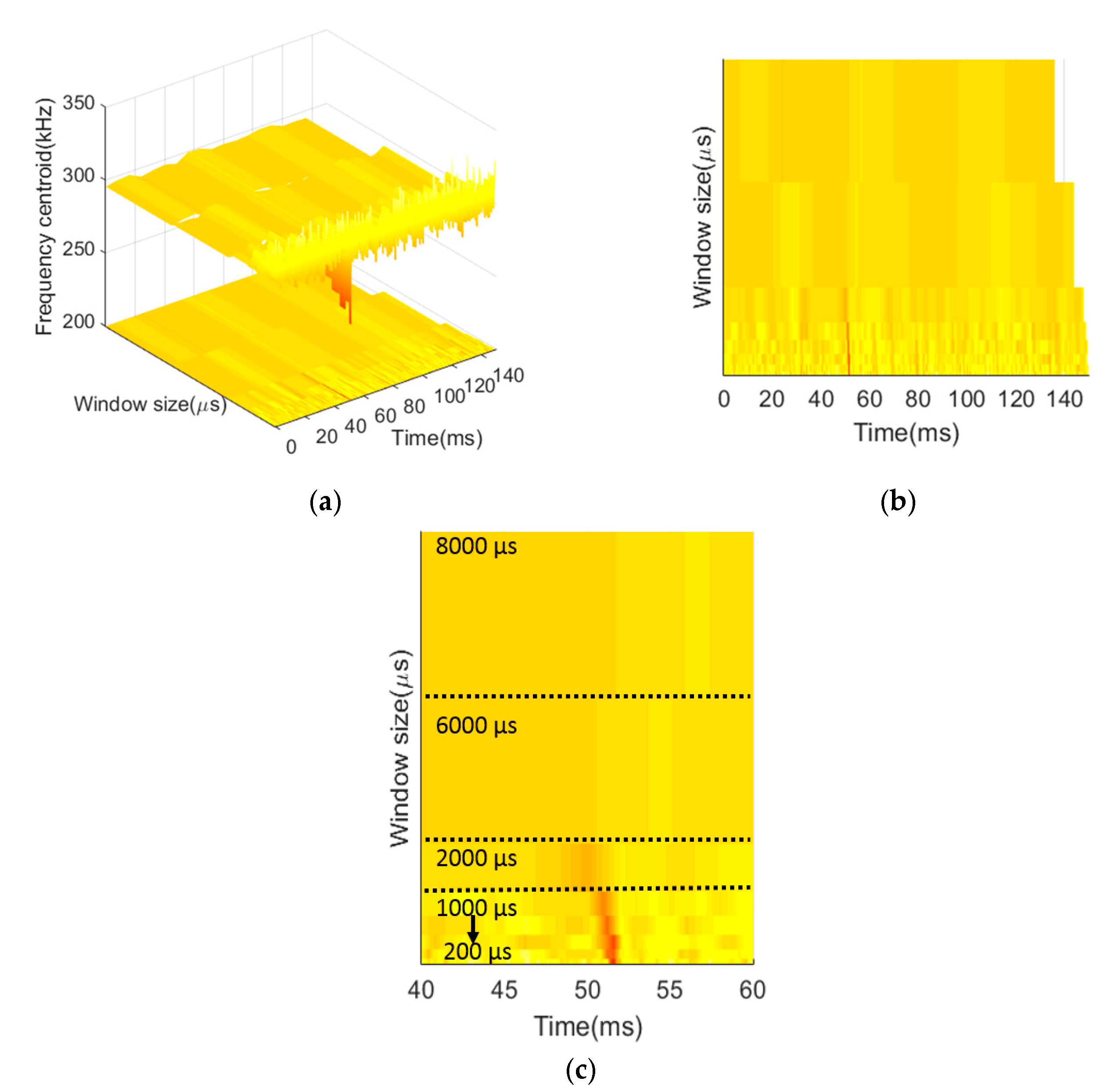
For improving the efficiency of signal processing method, a larger window size is preferable to reduce the computational time. The window size is increased up to 8 ms, and the SNR is kept the same as 1.0. It is identified that if the window size is larger than 2 ms, the background signal dominates the crack signal, as shown in Figure 15. The distinction between outlier and mean feature is reduced with the increase of window size.
While small window size improves the resolution of crack detection, large window size can reduce the computational cost of the identification process. Figure 16 shows the prediction error and the number of windows used to divide the streamed waveform. The predicted error is calculated by
where is the predicted embedded time and is the actual embedded time. While Figure 15 indicates that the window size of 200 μs has more indicative change in the spectra of frequency centroid, the minimum error is at the window size of 1 ms as this is the duration of the embedded crack signal. It is recommended to have the window size less than 1 ms, as typical AE signals due to the fatigue crack growth in metals have short duration.
4.3. The Application of Signal Decomposition to the NAVAIR Test Rig
In the previous section, the decomposition of streamed signal is shown to detect the crack signal with the proper selection of the window size. The smaller the window size is used, the more accurate the crack detection is achieved. Therefore, in this section, different window sizes are applied to the streamed signals that were recorded from the NAVAIR test rig. It is important to note that the complexity of gearbox structure, source mechanisms, and AE method causes the AE source identification highly challenging. The purpose is to identify the unusual AE signals (typically burst types) that are embedded into the streamed signals as outliers, which indicate the divergence from the normal operation. Fifteen (15) streamed waveforms are selected from the acoustically stable times of each testing day (the experiments are started in mornings and ended in about 3–4 h). The streamed signals are decomposed with different window sizes of 6 ms, 2 ms, and 1 ms. The frequency centroid is extracted from each window. In order to reduce the influence of operational condition, the frequency centroid is normalized to each mean value.
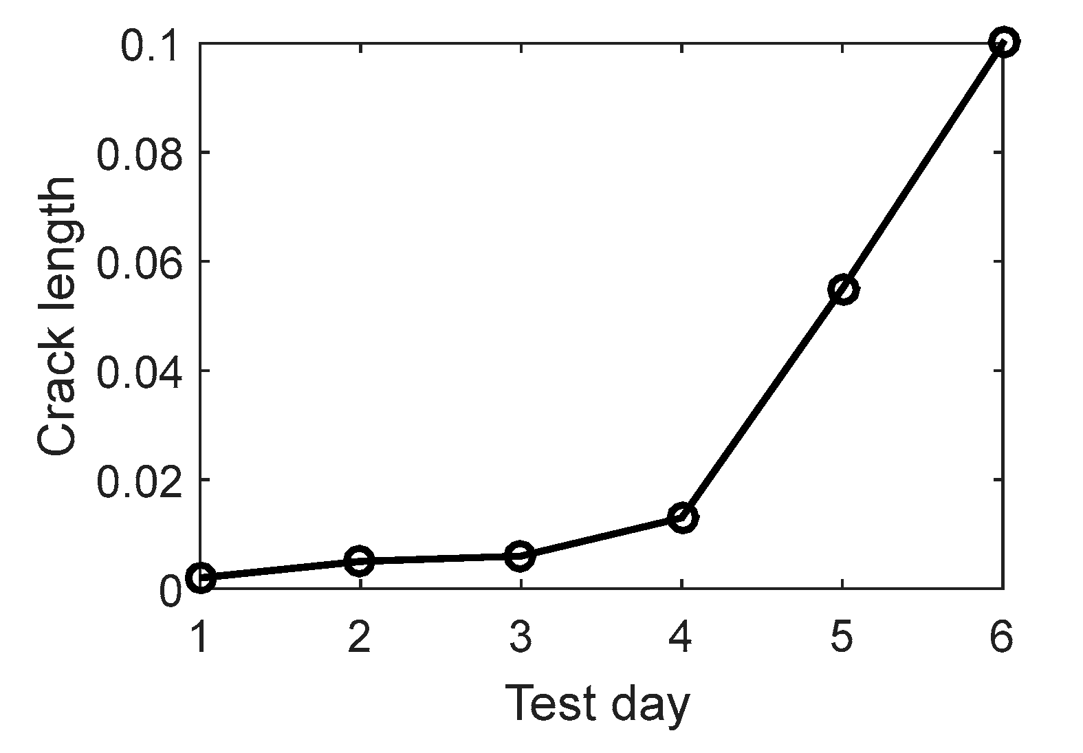
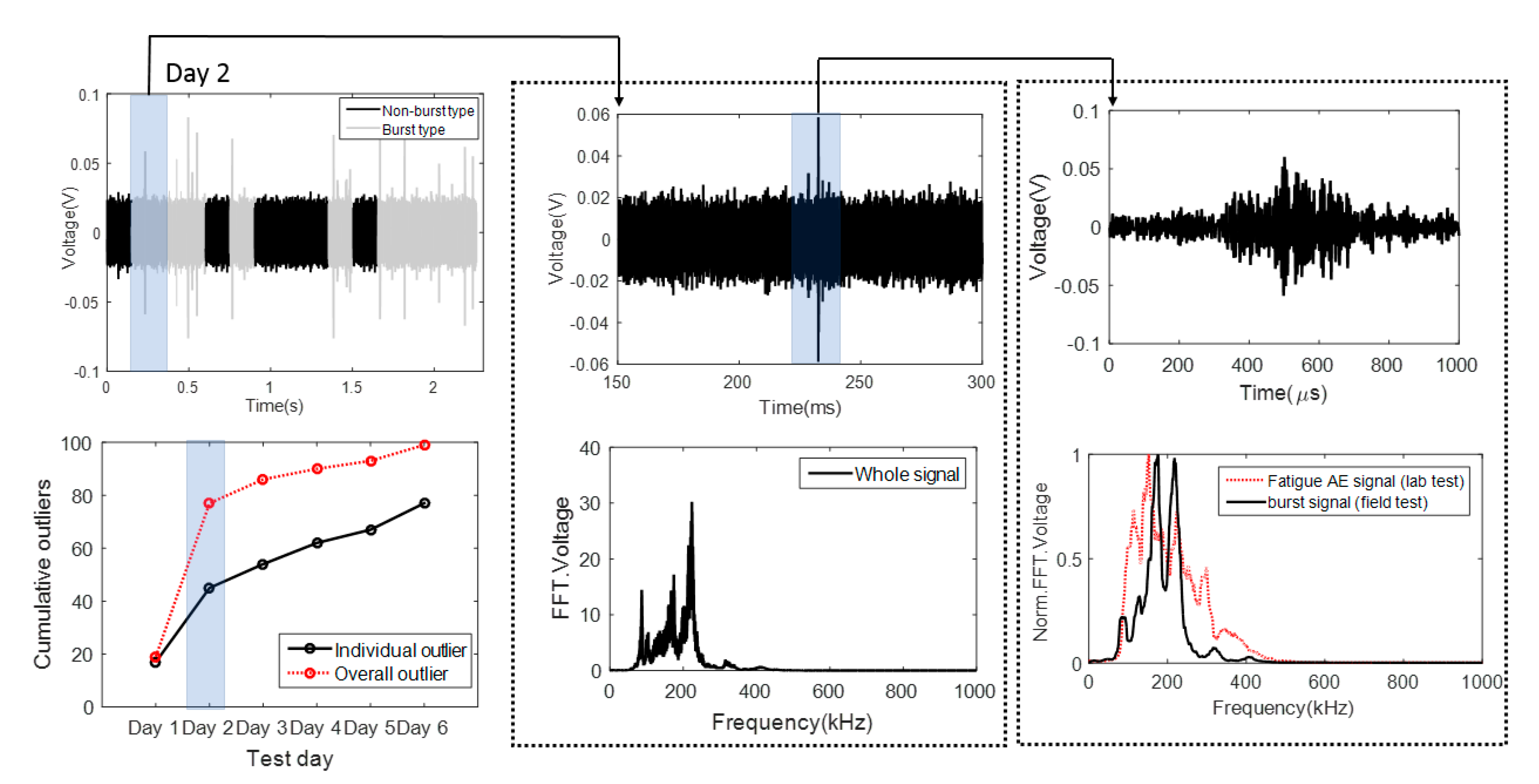
The outliers are determined as the AE data outside the dashed blue lines, as shown in Figure 17. The overall outlier considers the mean value of all data recorded throughout from day 1 to day 6. The individual outlier considers the mean value of individual day and identifies the limits for the outlier per day. As shown in Figure 17, both methods of outlier identification have similar cumulative outliers. With the decrease of window size, more outliers are observed, especially in the test day 2. The streamed signals from the test day 2 are plotted in Figure 18. There are several burst signals that are detected inside the streamed signals. The windowed frequency spectra using 1 ms duration indicate the peak frequency and the frequency centroid values are 152 kHz and 230 kHz, respectively. The values are similar to the characteristics of crack signal obtained in the laboratory. The crack size is measured using replica, and is shown in Figure 19. The crack grows gradually until the test day 4 and then exponentially. The crack length data of test days 2, 3, 4, and 6 are measured from the replica inserted into the gearbox; the data of test day 5 is obtained by curve fit. It is important to note that the test duration of each day is about 3–4 h, where above 2000 streamed waveforms are recorded. In this paper, only 15 streamed waveforms per day are analyzed. Therefore, the exponential change in the crack length cannot be observed from the outlier plots in Figure 17. The AE method cannot detect the crack size; however, it can predict the presence of unusual behavior in data, which can be used as the indication for performing more quantitative nondestructive evaluation methods.
5. Conclusions
In this paper, a decomposition approach of the streamed AE signals is developed in order to distinguish the crack related characteristics (i.e., burst signals) and the background noise characteristics. As the time-dependent waveform recording is based on the theory that the crack related AE signal is embedded into the streamed AE signal, it is important to identify the proper time window for extracting AE features. Using the NAVAIR gearbox simulator as representative noise signal and the laboratory scale UIC fatigue test of the planar spline section as representative crack signal, then the minimum window size for extracting the crack information is determined as 1 ms. The decomposition approach of the streamed AE signals is demonstrated on the identification of burst signals that are embedded into the streamed signals obtained from the spline testing of the gearbox simulator at the NAVAIR test rig. While the AE method cannot detect the crack size, it can indicate the presence of unusual behavior in highly noisy environments when the time-dependent waveform streaming approach is implemented.
Acknowledgments
This material is based upon work supported by the U.S. Naval Air Systems Command (NAVAIR) under Contract No. N68335-13-C-0417 entitled “Hybrid State-Detection System for Gearbox Components” awarded to the Metis Design Corporation. The authors would like to acknowledge the Research Open Access Publishing (ROAAP) Fund of the University of Illinois at Chicago for financial support towards the open access publishing fee for this article. The authors also would like to thank Seth Kessler and Gregory James for their inputs on the design of the test specimen. C-SAM equipment was acquired by DoD Equipment Contract No. W911NF-16-1-0500. Any opinions, findings and conclusions or recommendations expressed in this material are those of the authors and do not necessarily reflect the views of NAVAIR.
Author Contributions
Lu Zhang and Didem Ozevin conducted the laboratory experiments and analyzed the data recorded in laboratory and NAVAIR facility. David He provided inputs in the analysis of waveform streaming data, and embedding crack signal into the streamed data. William Hardman and Alan Timmons performed the NAVAIR gearbox experiments at the NAVAIR facility and provided feedback on fatigue experiments and data processing.
Conflicts of Interest
The authors declare no conflict of interest.
References
- Eftekharnejad, B.; Addali, A.; Mba, D. Shaft crack diagnostics in a gearbox. Appl. Acoust. 2012, 73, 723–733. [Google Scholar] [CrossRef]
- Yesilyurt, I.; Gu, F.; Ball, A.D. Gear tooth stiffness reduction measurement using modal analysis and its use in wear fault severity assessment of spur gears. NDT E Int. 2003, 36, 357–372. [Google Scholar] [CrossRef]
- Eftekharnejad, B.; Mba, D. Monitoring natural pitting progress on helical gear mesh using acoustic emission and vibration. Strain 2011, 47, 299–310. [Google Scholar] [CrossRef]
- Zhu, X.; Zhong, C.; Zhe, J. A high sensitivity wear debris sensor using ferrite cores for online oil condition monitoring. Meas. Sci. Technol. 2017, 28, 75102. [Google Scholar] [CrossRef]
- Dempsey, P.J. Integrating Oil Debris and a High Sensitivity Wear Debris Sensor Using Ferrite Cores for Online Oil Condition Monitoring Vibration Measurements for Intelligent Machine Health Monitoring. Ph.D. Thesis, Toledo University, Toledo, OH, USA, 2003. [Google Scholar]
- Li, R.; He, D. Rotational machine health monitoring and fault detection using EMD-based acoustic emission feature quantification. IEEE Trans. Instrum. Meas. 2012, 61, 990–1001. [Google Scholar] [CrossRef]
- Ozevin, D.; Dong, J.; Godinez, V.; Carlos, M. Damage assessment of gearbox operating in high noisy environment using waveform streaming approach. J. Acoust. Emiss. 2007, 25, 355–363. [Google Scholar]
- Loutas, T.H.; Roulias, D.; Pauly, E.; Kostopoulos, V. The combined use of vibration, acoustic emission and oil debris on-line monitoring towards a more effective condition monitoring of rotating machinery. Mech. Syst. Signal Process. 2011, 25, 1339–1352. [Google Scholar] [CrossRef]
- Li, C.J.; Lee, H.; Choi, S.H. Estimating size of gear tooth root crack using embedded modelling. Mech. Syst. Signal Process. 2002, 16, 841–852. [Google Scholar]
- Samuel, P.D.; Pines, D.J. A review of vibration-based techniques for helicopter transmission diagnostics. J. Sound Vib. 2005, 282, 475–508. [Google Scholar] [CrossRef]
- Hase, A.; Mishina, H.; Wada, M. Correlation between features of acoustic emission signals and mechanical wear mechanisms. Wear 2012, 292, 144–150. [Google Scholar] [CrossRef]
- Li, R.; Seçkiner, S.U.; He, D.; Bechhoefer, E.; Menon, P. Gear fault location detection for split torque gearbox using AE sensors. IEEE Trans. Syst. Man Cybern. Part C Appl. Rev. 2012, 42, 1308–1317. [Google Scholar] [CrossRef]
- Gu, D.; kim, J.; An, Y.; Choi, B. Detection of faults in gearboxes using acoustic emission signal. J. Mech. Sci. Technol. 2011, 25, 1279–1286. [Google Scholar] [CrossRef]
- Wang, W. An enhanced diagnostic system for gear system monitoring. IEEE Trans. Syst. Man Cybern. Part B 2008, 38, 102–112. [Google Scholar] [CrossRef]
- Zhang, L.; Yalcinkaya, H.; Ozevin, D. Numerical Approach to Absolute Calibration of Piezoelectric Acoustic Emission Sensors using Multiphysics Simulations. Sens. Actuators A Phys. 2017, 256, 12–23. [Google Scholar] [CrossRef]
- Zhang, L.; Ozevin, D.; Hardman, W.; Timmons, A. Acoustic emission signatures of fatigue damage in idealized bevel gear spline for localized sensing. Metals 2017, 7, 242. [Google Scholar] [CrossRef]
- Oppenheim, A.V. Discrete-Time Signal Processing; Pearson Education India: Chennai, India, 1999; ISBN 8131704920. [Google Scholar]
Figure 1.
The Naval Air Systems Command (NAVAIR) gearbox test (a) the test rig, and (b) the types and positions of the AE sensors on the gearbox housing (CH (Channel) 1 and 2 are WD (wideband) sensors, and CH 3 and 4 are micro 30 sensors) (c) the sensitivity curves of Micro30s and WD sensor provided by Mistras Group Inc.

Figure 2.
The UIC fatigue test, (a) the loading machine with the sample, (b) the planar spline sample and dimensions, and (c) the positions of AE sensors and strain gauge.
Figure 2.
The UIC fatigue test, (a) the loading machine with the sample, (b) the planar spline sample and dimensions, and (c) the positions of AE sensors and strain gauge.
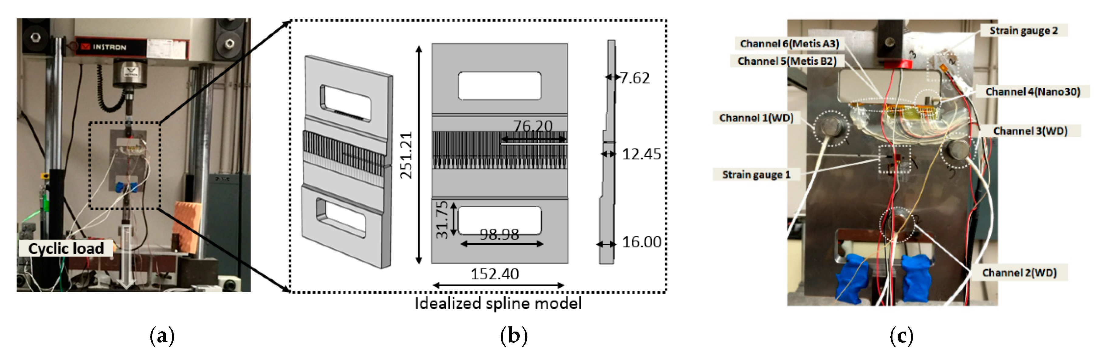
Figure 3.
The comparison of cracks directions in the NAVAIR gearbox test and the UIC fatigue test, (a) gear spline; (b) planar spline; (c) microscopic image of crack growth at the planar spline; and (d) the acoustic microscope image of the crack measured from the back surface of the planar spline.
Figure 3.
The comparison of cracks directions in the NAVAIR gearbox test and the UIC fatigue test, (a) gear spline; (b) planar spline; (c) microscopic image of crack growth at the planar spline; and (d) the acoustic microscope image of the crack measured from the back surface of the planar spline.
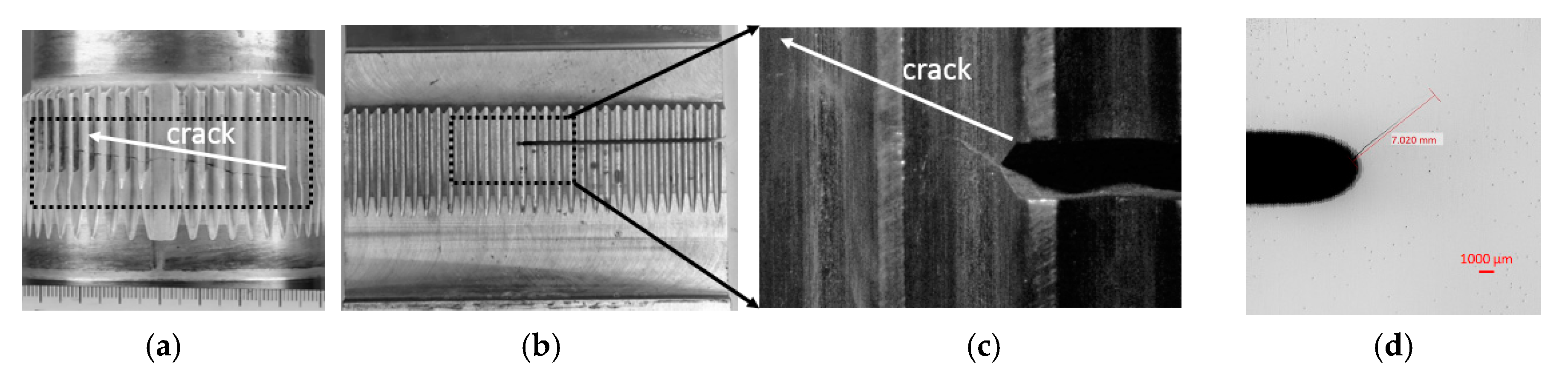
Figure 4.
Examples of AE signals and frequency spectra (a,b) streamed AE signal obtained from the NAVAIR gearbox test, (c,d) signals due to crack growth obtained from the UIC fatigue test, (e,f) signals due to the pencil lead break (PLB) testing obtained from the UIC fatigue test, and (g,h) the histograms of AE amplitudes from the NAVAIR gearbox test and the UIC fatigue test. FFT: fast Fourier transform.

Figure 5.
The window of 1 ms duration from the streamed acoustic emission (AE) signal of the NAVAIR gearbox test.
Figure 5.
The window of 1 ms duration from the streamed acoustic emission (AE) signal of the NAVAIR gearbox test.
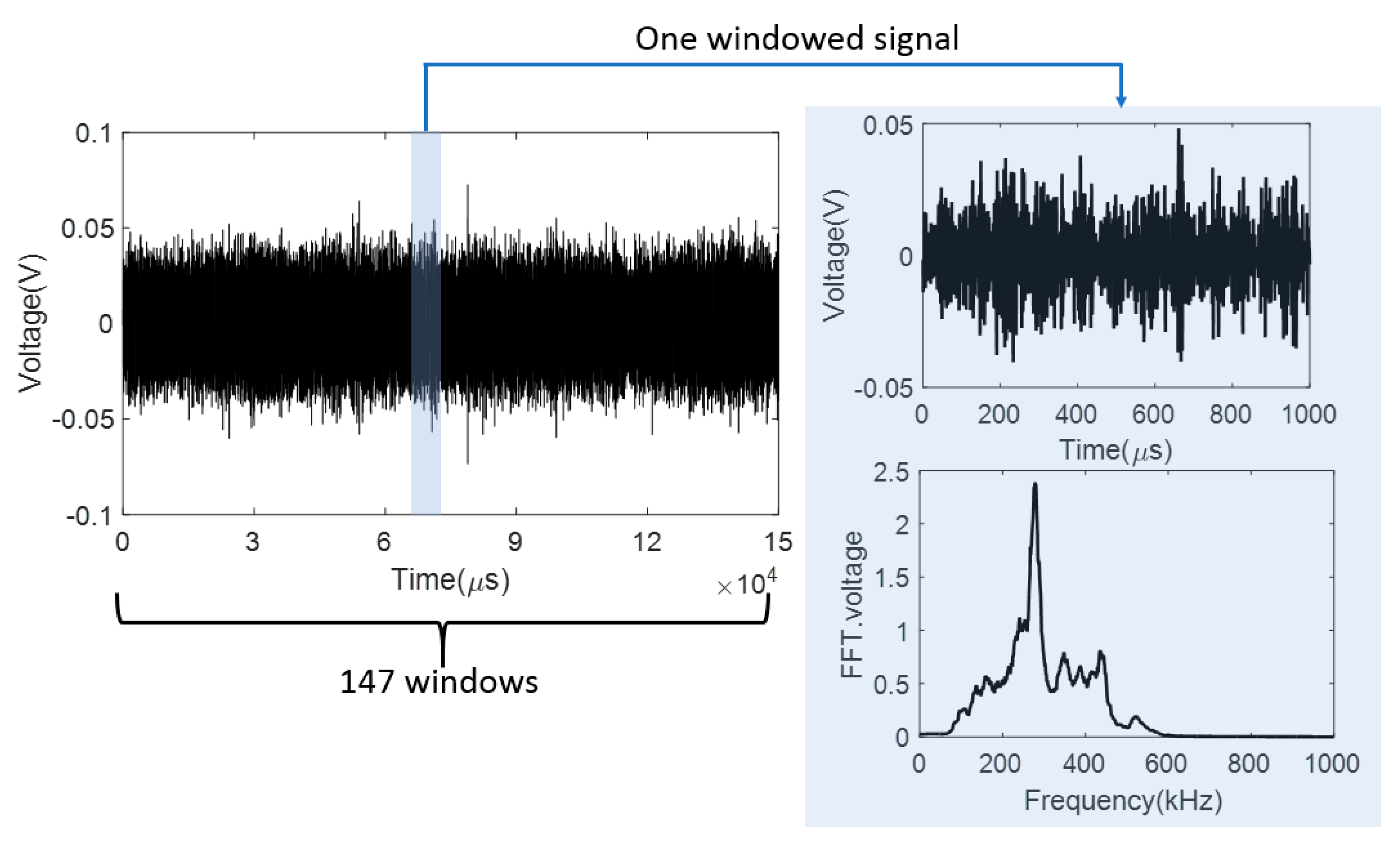
Figure 6.
The window to obtain the operational noise frequency of the UIC fatigue test.

Figure 7.
The statistical analysis of streamed signal without crack emission (a–c) the AE power, peak frequency and frequency centroid of each window, and (d–f) normal distribution of AE power, peak frequency and frequency centroid obtained from the windowed streamed signal.
Figure 7.
The statistical analysis of streamed signal without crack emission (a–c) the AE power, peak frequency and frequency centroid of each window, and (d–f) normal distribution of AE power, peak frequency and frequency centroid obtained from the windowed streamed signal.
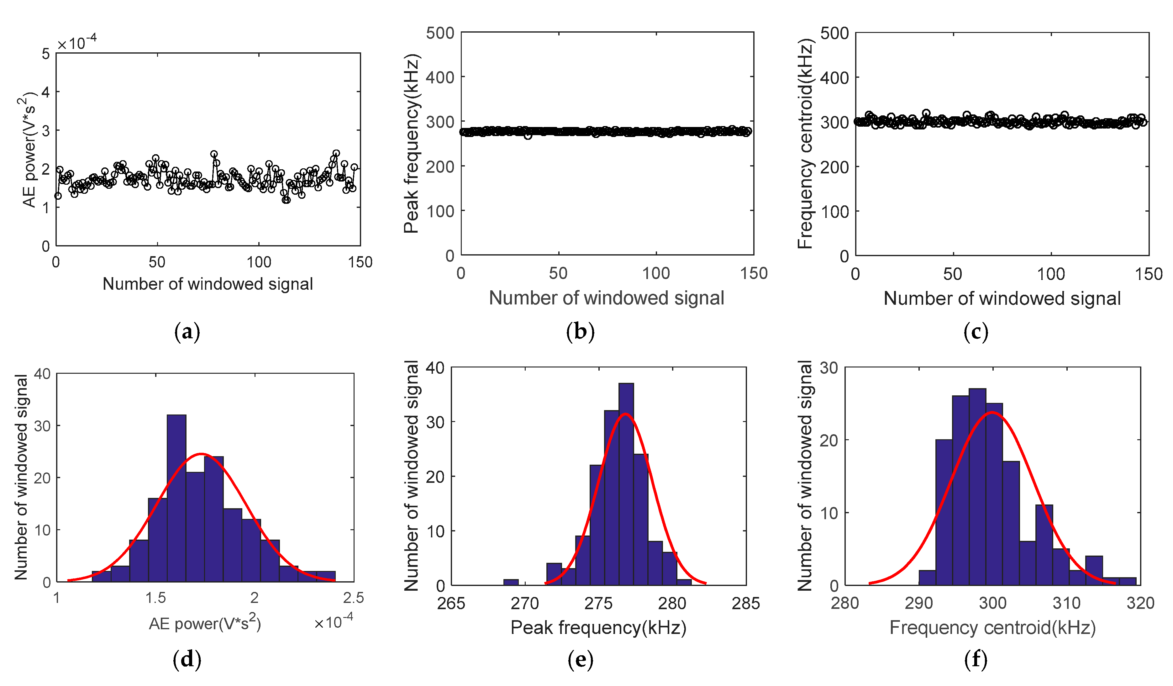
Figure 8.
The schematic of signal summation.

Figure 9.
The comparison of embedded cracking streamed signals, (a) SNR = 7.5, (b) SNR = 4.0, (c) SNR = 2.0, and (d) SNR = 1.0.
Figure 9.
The comparison of embedded cracking streamed signals, (a) SNR = 7.5, (b) SNR = 4.0, (c) SNR = 2.0, and (d) SNR = 1.0.
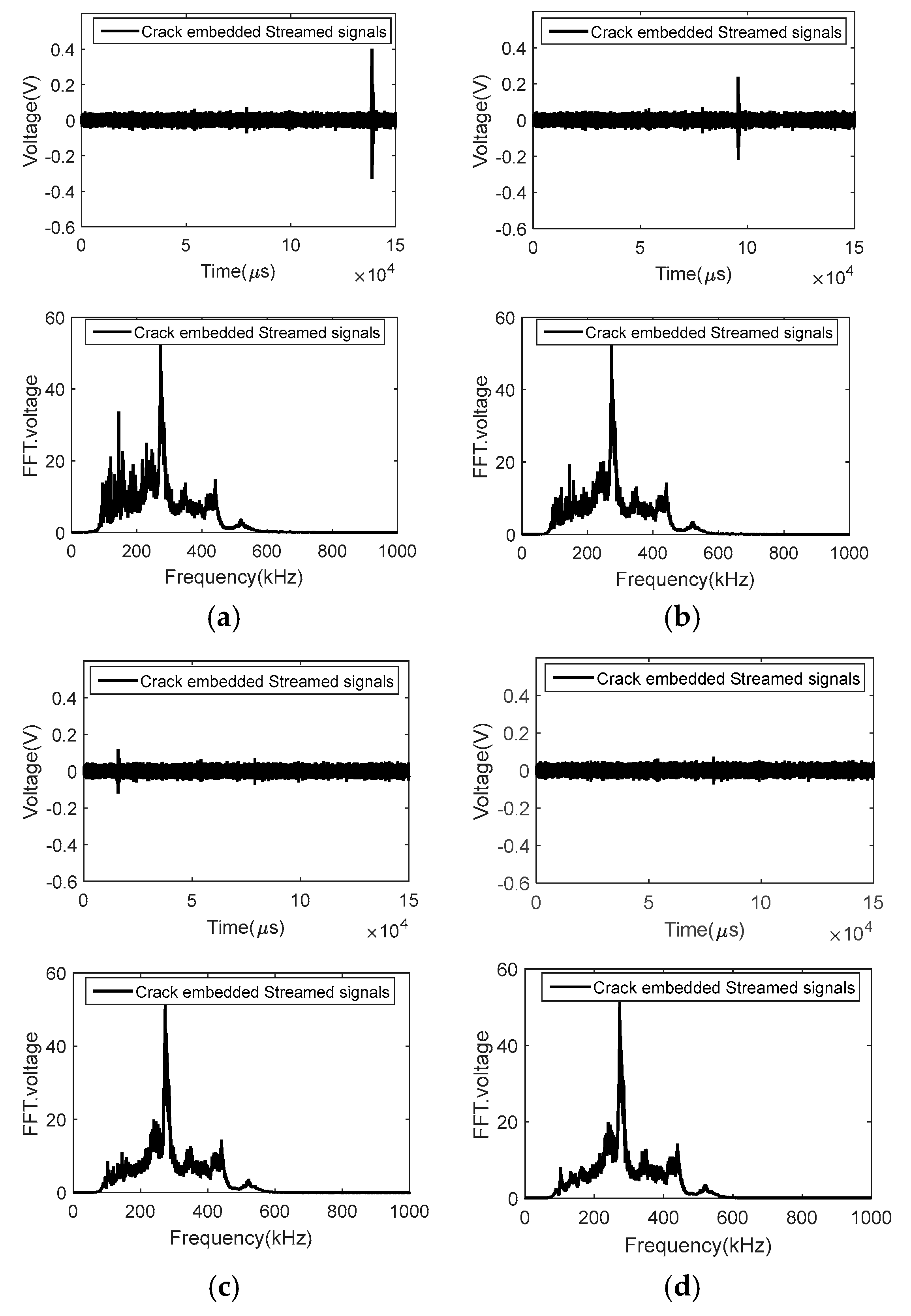
Figure 10.
The outlier detection of AE power, peak frequency and frequency centroid of original streamed signal and embedded streamed signal (SNR = 1.0, location of cracking signal: 74).
Figure 10.
The outlier detection of AE power, peak frequency and frequency centroid of original streamed signal and embedded streamed signal (SNR = 1.0, location of cracking signal: 74).

Figure 11.
The outlier detection of AE power, peak frequency and frequency centroid of original streamed signal and embedded streamed signal (SNR = 1.0, location of cracking signal: 120).
Figure 11.
The outlier detection of AE power, peak frequency and frequency centroid of original streamed signal and embedded streamed signal (SNR = 1.0, location of cracking signal: 120).
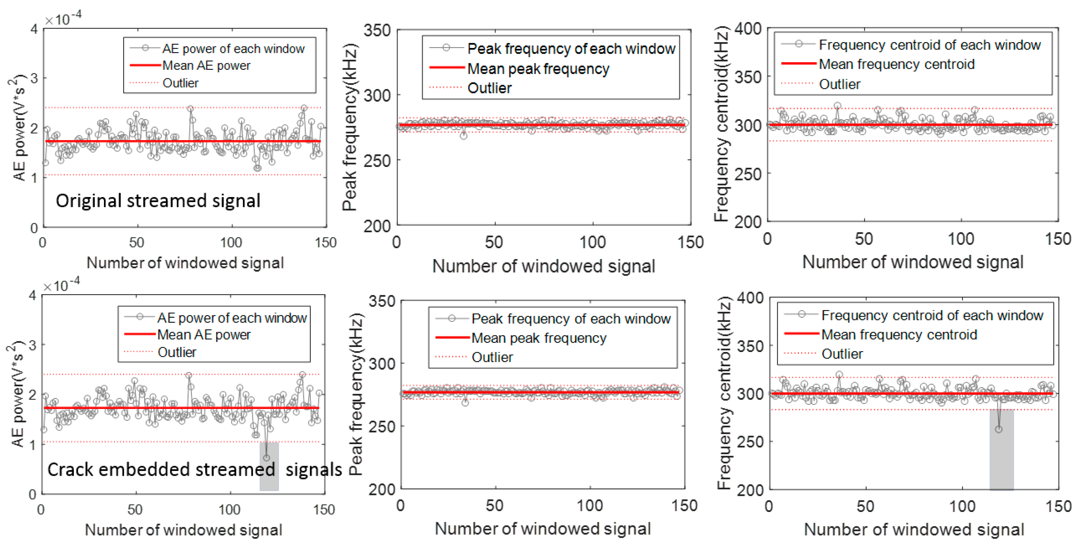
Figure 12.
The spectra of frequency centroid (unit: kHz), (a) embedded streamed signals (SNR = 1.0), (b) zoomed embedded stream signals, and (c) original streamed signals.
Figure 12.
The spectra of frequency centroid (unit: kHz), (a) embedded streamed signals (SNR = 1.0), (b) zoomed embedded stream signals, and (c) original streamed signals.

Figure 13.
The spectra of AE power (unit: V*s2), (a) embedded streamed signal (SNR = 1.0), (b) windowed embedded stream signal to 45–60 ms, and (c) original streamed signal.
Figure 13.
The spectra of AE power (unit: V*s2), (a) embedded streamed signal (SNR = 1.0), (b) windowed embedded stream signal to 45–60 ms, and (c) original streamed signal.
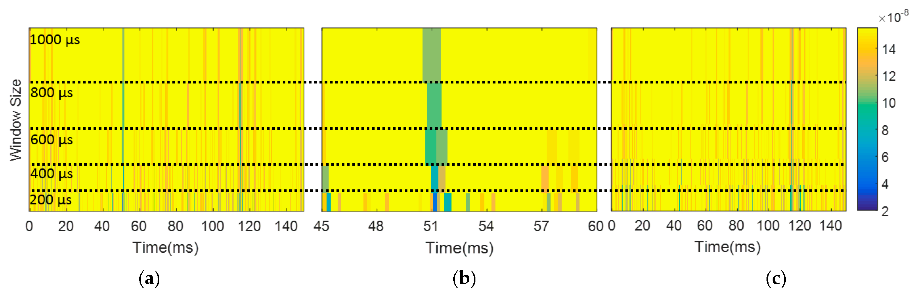
Figure 14.
The spectra of peak frequency (unit: kHz), (a) embedded streamed signal (SNR = 1.0), and (b) original streamed signal.
Figure 14.
The spectra of peak frequency (unit: kHz), (a) embedded streamed signal (SNR = 1.0), and (b) original streamed signal.
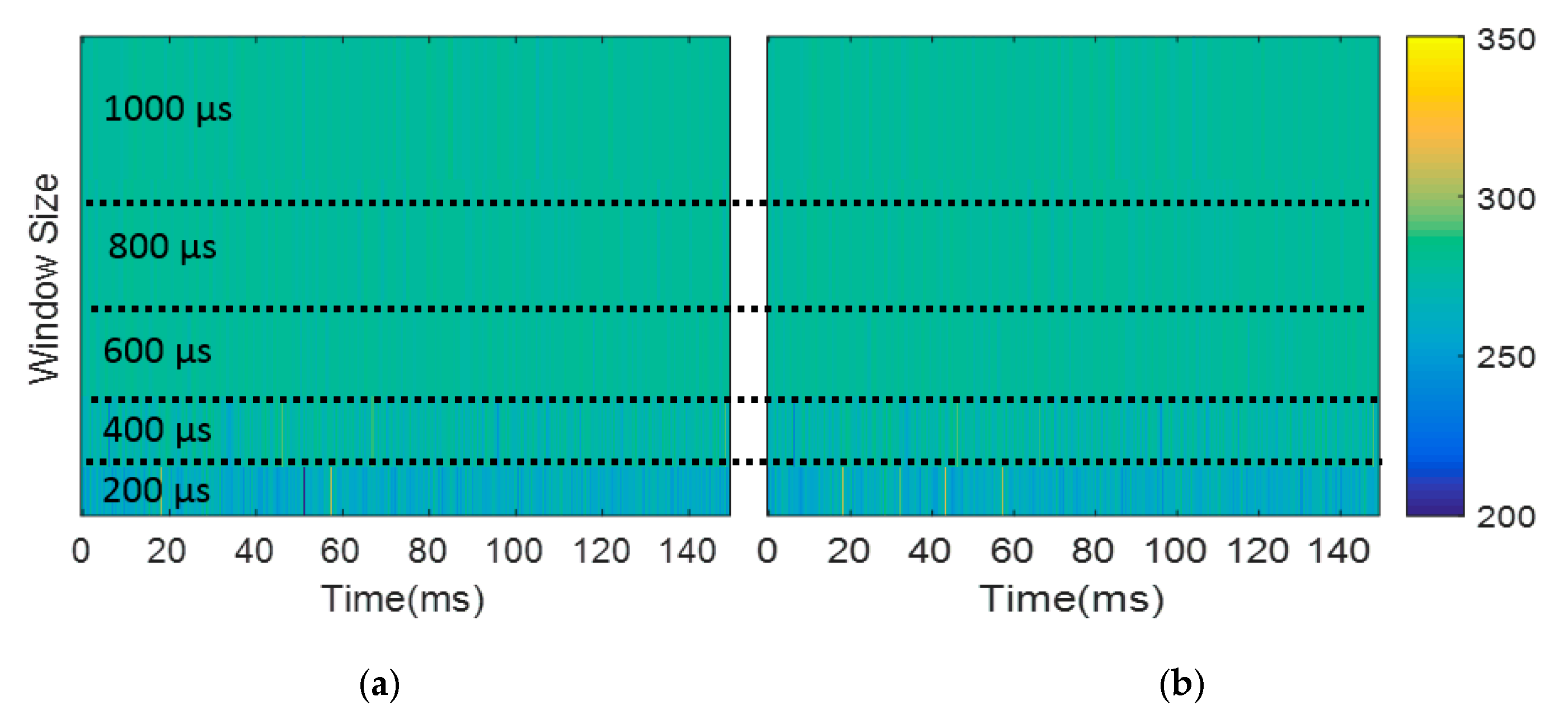
Figure 15.
The spectra of frequency centroid by selection of different window size, (a) three-dimensional (3D) suface plot (b) projected to xy plane, and (c) window of (b) with the time window of 40 ms to 60 ms.
Figure 15.
The spectra of frequency centroid by selection of different window size, (a) three-dimensional (3D) suface plot (b) projected to xy plane, and (c) window of (b) with the time window of 40 ms to 60 ms.

Figure 16.
The relation of the predicted error and the number of the windows in relation to the window size.
Figure 16.
The relation of the predicted error and the number of the windows in relation to the window size.
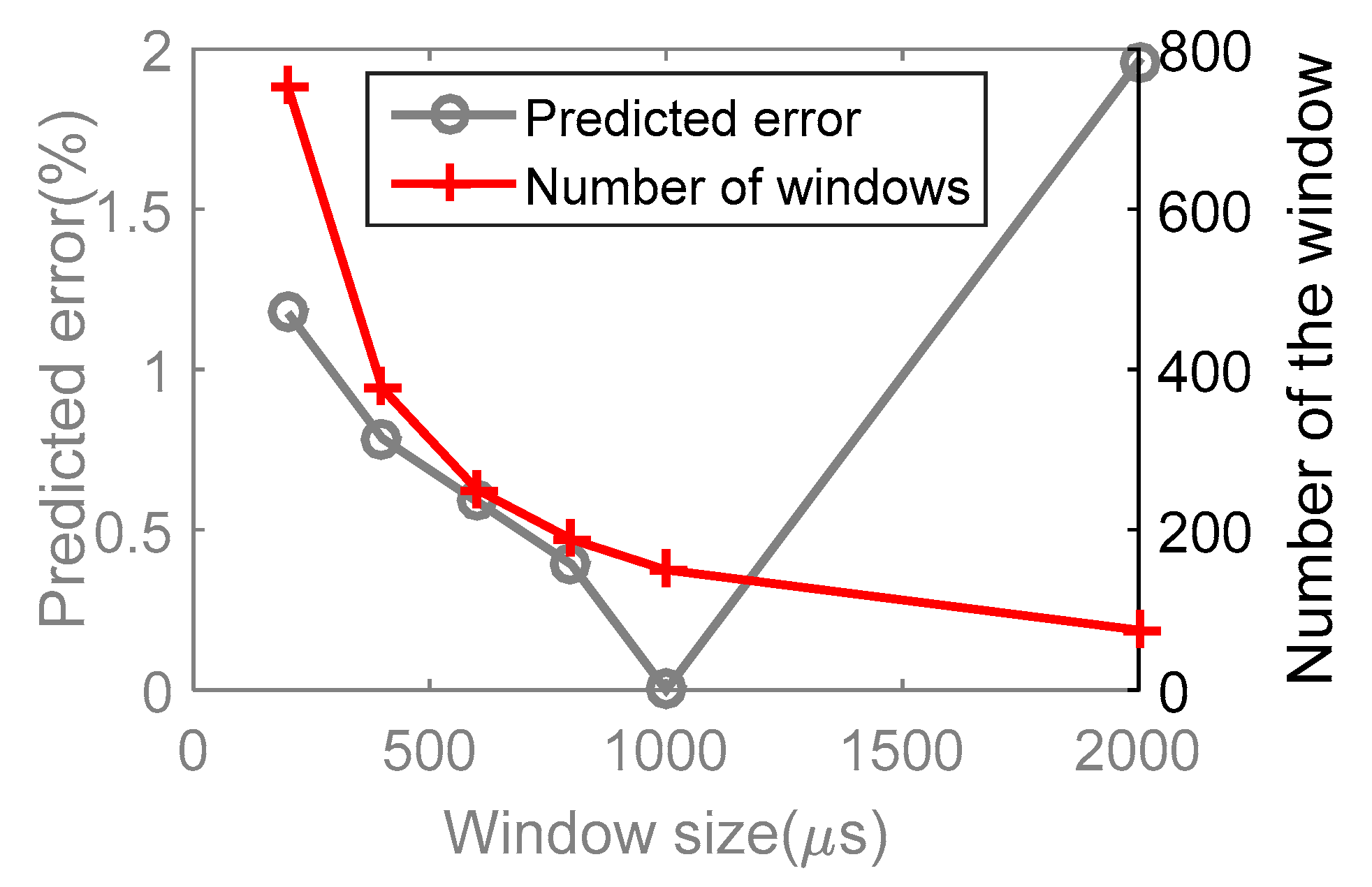
Figure 17.
The outlier prediction with different window sizes.
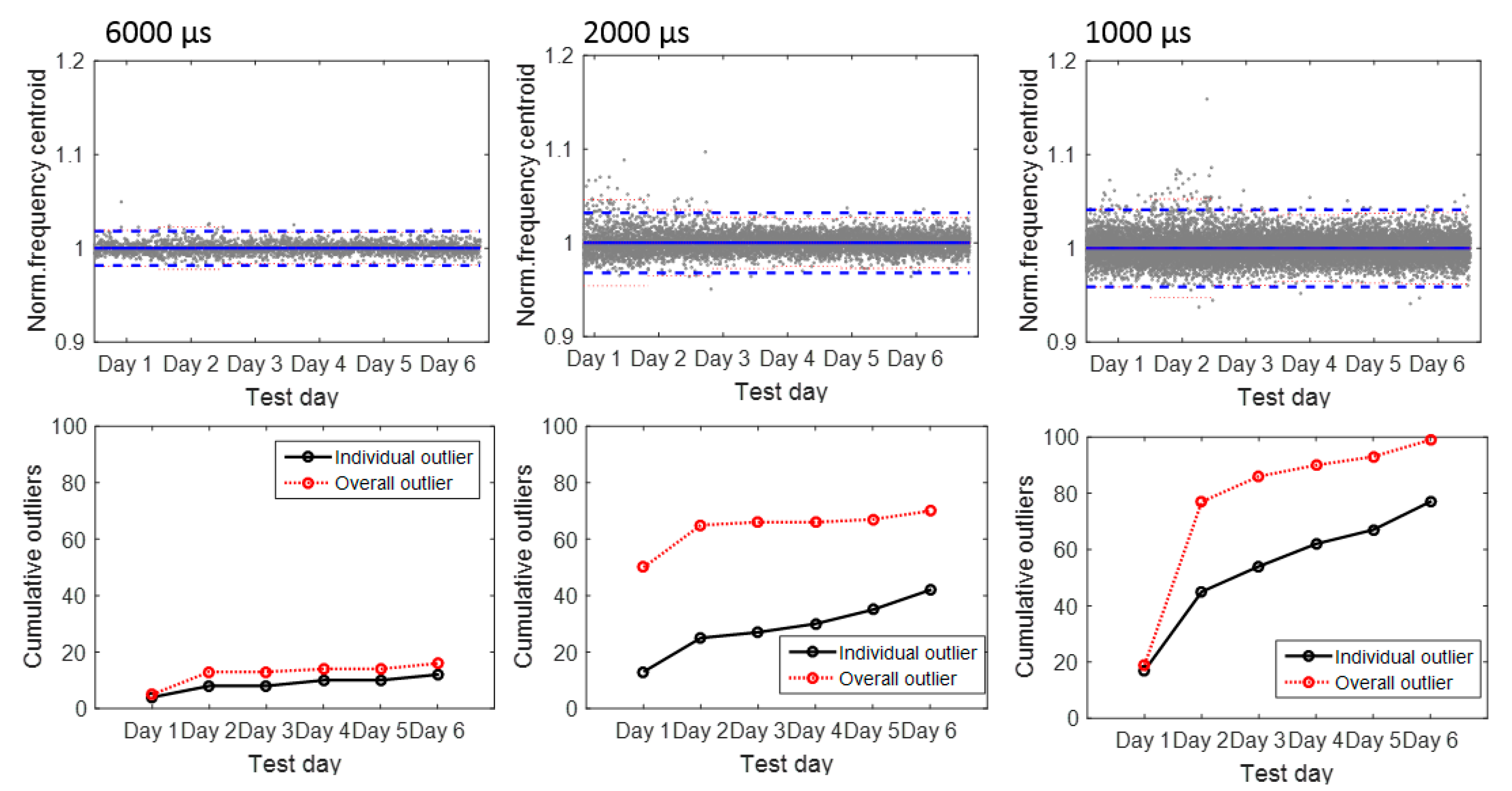
Figure 18.
The burst signals detected in the test day 2 and their frequency spectra using the windowed time histories.
Figure 18.
The burst signals detected in the test day 2 and their frequency spectra using the windowed time histories.

Figure 19.
The crack growth behavior of fatigue experiment conducted at the NAVAIR facility.

Table 1.
The comparison of Naval Air Systems Command (NAVAIR) gearbox test and UIC fatigue test.
| Test Type | Loading Condition | Sample Geometry | Sample Material | AE Sensor | Sensor Couplant | AE Sensor Position | Crack Direction |
|---|---|---|---|---|---|---|---|
| NAVAIR gearbox test | Hub moment | Cylinder spline gear | Structural steel | WD sensor | Vacuum grease | On the gearbox housing | Perpendicular to spline |
| UIC fatigue test | Tensile | Planar sample with splines | Structural steel | WD sensor | Super glue | On the planar sample | Perpendicular to spline |
Table 2.
The summary of Acoustic Emission (AE) features.
| Signal Source | AE Signal Power (V*s2) | AE Peak Frequency (kHz) | AE Frequency Centroid (kHz) |
|---|---|---|---|
| Entire streamed signal | 0.000173 | 273 | 295 |
| Windowed streamed signal | 0.000174 | 277 | 300 |
| Crack growth | 0.0731 | 152 | 230 |
| Pencil lead break (PLB) source | 0.4335 | 228 | 255 |
| Noise of fatigue test | 0.0013 | 234 | 268 |
© 2017 by the authors. Licensee MDPI, Basel, Switzerland. This article is an open access article distributed under the terms and conditions of the Creative Commons Attribution (CC BY) license (http://creativecommons.org/licenses/by/4.0/).
Share and Cite
MDPI and ACS Style
Zhang, L.; Ozevin, D.; He, D.; Hardman, W.; Timmons, A. A Method to Decompose the Streamed Acoustic Emission Signals for Detecting Embedded Fatigue Crack Signals. Appl. Sci. 2018, 8, 7. https://doi.org/10.3390/app8010007
AMA Style
Zhang L, Ozevin D, He D, Hardman W, Timmons A. A Method to Decompose the Streamed Acoustic Emission Signals for Detecting Embedded Fatigue Crack Signals. Applied Sciences. 2018; 8(1):7. https://doi.org/10.3390/app8010007
Chicago/Turabian StyleZhang, Lu, Didem Ozevin, David He, William Hardman, and Alan Timmons. 2018. "A Method to Decompose the Streamed Acoustic Emission Signals for Detecting Embedded Fatigue Crack Signals" Applied Sciences 8, no. 1: 7. https://doi.org/10.3390/app8010007
Note that from the first issue of 2016, this journal uses article numbers instead of page numbers. See further details here.