Placing Visual Sensors Using Heuristic Algorithms for Bridge Surveillance


1
School of Industrial Engineering, Purdue University, West Lafayette, IN 47907, USA
2
Department of Industrial & Management Engineering/Intelligence & Manufacturing Research Center, Kyonggi University, Suwon, Gyeonggi 16227, Korea
3
Korea Railroad Research Institute, Uiwang, Gyeonggi 16105, Korea
*
Author to whom correspondence should be addressed.
Appl. Sci. 2018, 8(1), 70; https://doi.org/10.3390/app8010070
Submission received: 1 November 2017
/
Revised: 20 December 2017
/
Accepted: 3 January 2018
/
Published: 6 January 2018
(This article belongs to the Special Issue Advanced Internet of Things for Smart Infrastructure System)
Abstract
:This study addresses the camera placement problem for bridge surveillance and proposes solutions that minimize the cost while satisfying the minimum coverage level. We discuss the field of view of cameras in the three-dimensional space. We also consider occlusions, the characteristics of surveillance targets, and different pan-tilt-zoom cameras in the visibility test. To solve the camera placement problem while minimizing the total cost, we propose a genetic algorithm (GA) and a uniqueness score with a local search algorithm (ULA). Problem sets for a large-scale dimension scenario are generated based on the data of actual bridges in the Republic of Korea. For three simulation sets and a case study of Samoonjin Bridge, the proposed ULA yields better results than GA.
1. Introduction
The increasing social demand for disaster-recovery systems has resulted in an increasing requirement for surveillance activities in core-infrastructure components. In the case of a natural disaster such as a flood or an earthquake, the infrastructure near the river—the bridges, in particular—plays an important role in the delivery of supplies to victims and in the repair of the damaged area in a timely manner. The placement of visual surveillance devices, such as a camera, can directly impact not only the total cost but also the coverage of surveillance targets. In this respect, the development of efficient algorithms for deploying cameras allows a detailed evaluation of damages sustained by a bridge within budget constraints. Algorithms also enable surveillance applications that require quick pre-emptive deployment when budget constraints and occluded points caused by static or dynamic obstacles change over time. In order to take into account more detailed scenarios, a quick computation time is crucial to find a new camera configuration in response to or to accommodate such changes.
However, the development of an algorithm for the camera placement problem poses two challenges. The first challenge is the computational complexity of the problem. The combinatorial optimization problem of identifying the optimal placement of multiple cameras to observe the maximum space is NP-hard [1]. Particularly, in the case of placing cameras to monitor large infrastructures, the size of the problem and the number of decision variables increase as the number of feasible locations for the camera and the number of grid points increase due to the nature of the NP-hard problem. To address this issue, we present the visibility test with a minimum coverage level to efficiently reduce the search space. We present two well-known heuristic algorithms: a greedy algorithm and genetic algorithm. The greedy algorithm finds a solution from the myopic perspective and is commonly used in previous literature [2,3]. Genetic algorithms (GA) are widely used to solve the camera placement problem because these algorithms can probe the solution space and locate optima quickly with no prior information [4]. We also propose a new heuristic algorithm inspired by the uniqueness score, which puts a higher importance on a grid point of the target that is frequently left uncovered by other cameras. After finding an initial solution based on the sum of uniqueness scores, a local search phase improves it by changing the types of cameras chosen to reduce the total cost within the minimum coverage level. To validate the performance of the probabilistic search methods, we designed simulation experiments and compared the performance of the proposed algorithm with those of two well-known heuristic algorithms: a greedy algorithm and a genetic algorithm. The performance of the algorithm was measured by the average coverage from the experiments.
The second challenge is related to the geographical features of the areas near bridges. In addition to the characteristics of the typical camera placement problem, the surveillance of bridges involves additional constraints related to the possible locations of the camera and occlusions. For example, because of the presence of rivers and the height of bridges, the areas where cameras can be placed are highly restricted to riverside areas or narrow areas on the bridges. Due to the rectangular shape of bridges, particularly the planes and edges, a part of the camera’s view is obstructed and the underside of the bridge cannot be observed, despite the broader field of view of pan-tilt-zoom (PTZ) cameras. The occluded view of the camera, the restricted areas, and the broader field of view of the PTZ cameras result in an increased computation time and memory usage for the camera placement problem due to the higher number of possible configurations, overlapped areas, and occluded points. Thus, considering these constraints and developing algorithms to arrive at the efficient placement of cameras within a reasonable timeframe constitutes a significant step toward increasing the scope of applications in the field. To address these constraints, we first define the characteristics of PTZ cameras, restricted areas, and occlusions. Further, we propose an approach to quantize the search space into many finite candidate placements, considering the limitations of memory size. We also design simulation problem sets to consider various deployment scenarios and to experimentally evaluate our approach based on the data of bridges in the Republic of Korea. In addition, we present a case study of a real bridge in Korea with actual data.
The remainder of this manuscript is organized as follows: In Section 2, we review previous research related to camera placement problems; in Section 3, we describe the characteristics of the camera placement problem with the help of basic definitions and assumptions; in Section 4, we present three heuristic algorithms to solve the defined problem; in Section 5, we describe experiments conducted to verify the validity of our approach and summarize the experimental results; and in Section 6, we present the conclusion and discuss possible extensions of our study.
2. Literature Review
The camera placement problem is closely related to the art gallery problem (AGP), which is the problem of determining the minimum number of guards required to cover the interior of an art gallery [5]. The AGP assumes that all guards have similar capabilities and unlimited visibility, which implies an infinite visual distance. However, realistically, the visibility of a camera is limited by its visual distance and visual angle, and a camera placement problem with identical cameras rarely exists. Furthermore, various constraints, including various types of cameras having different specifications and occlusions, further complicate the camera placement problem, where even a three-dimensional AGP is NP-hard [6]. Table 1 summarizes the existing literature on this problem, which it categorizes by space, objective function, and the approach of the solution.
In terms of objective functions, the maximization of coverage has been widely studied and many solution approaches have been suggested [2,3,4,7,8,9,11,12,13,14,15,16]. Furthermore, multi-objective problems, including maximizing coverage and visibility while minimizing the total cost, have been studied [10,11]. However, the camera placement problems with an objective of maximizing coverage under a cost constraint or minimizing cost under a coverage constraint in multi-camera systems are usually far less studied [18].
With respect to solution approaches to the camera placement problem, mathematical approaches have achieved better performances than other heuristic methods. Yabuta and Kitazawa [8] formulated a problem for effective camera locations in 2D space. They proposed binary integer programming (BIP) to minimize the cost of sensors to completely cover the sensor field. However, even though optimization software capable of solving BIP problems exists, the extremely long calculation time needed for larger problems makes it impractical to obtain an exact solution for any reasonable-sized camera placement problem.
For this reason, heuristic or meta-heuristic algorithms have been applied to obtain good solutions within a reasonable amount of time. Hörster and Lienhart [2] proposed a greedy algorithm and dual sampling algorithm to maximize the coverage provided by a given number of cameras and minimize the total price of the sensor array. Fleishman et al. [10] developed a greedy algorithm based on an image-based model for the automatic camera placement problem in 3D space. To maximize the weighted coverage, Jun et al. [15] proposed a collaboration-based local search algorithm (COLSA) for the camera placement problem in 3D space.
In particular, evolutionary algorithms, including particle swarm optimization (PSO), simulated annealing (SA), and the genetic algorithm (GA), have been widely used to solve the camera placement problems. To maximize weighted coverage for different sub-regions, Jiang et al. proposed a novel coverage-enhancement algorithm that included an occlusion-free surveillance model based on GA [9]. Morsly et al. [17] proposed a binary particle swarm optimization (BPSO) algorithm to solve the camera network placement problem based on simulation results for 2D and 3D scenarios. Ma et al. also proposed a 3D directional-sensor coverage-control model with tunable orientations, and they developed an SA-based algorithm to enhance area coverage. Belhaj et al. [10] compared the use of the non-dominated sorting genetic algorithm (NSGA-II) and the covariance matrix adaptation-evolution strategy (CMA-ES) to address the multi-objective sensor placement problem.
In addition to solution approaches, various constraints have been studied, including PTZ cameras and occlusions. Indu et al. [19] addressed the camera placement problem by using various cameras to maximize the coverage of user-defined priority areas with the optimum values of parameters that included pan, tilt, zoom, and camera location. Piciarelli et al. [20] addressed two issues common in surveillance applications: occlusions and the reconfiguration of PTZ cameras. They also considered new relevance maps, which are computed by identifying the occluded areas for each camera.
Although numerous camera placement problems have been studied, only a few studies have investigated the problem in the context of large-scale surveillance in the 3D space and using real-world data. Furthermore, studies addressing the camera placement problem with different specifications of PTZ cameras and occlusions are rare in the literature. Therefore, the goal of our study is to bridge the gap between theoretical studies and real-world problems that have more realistic requirements for surveillance activities. In this manuscript, Section 3 describes the constraints, including PTZ cameras, occlusions, and the characteristics of the surveillance targets. Section 4 presents efficient algorithms for solving the problem within a reasonable amount of time in a scenario.
3. Problem Definition
In this section, we address the camera placement problem in three-dimensional (3D) space by using discrete areas; this approach optimizes the total cost of different cameras while satisfying the minimum coverage level. The minimum coverage level is closely related to the minimum number of cameras required, and therefore, affects the total cost [21]. First, we define the field of view (FoV) model of a PTZ camera in 3D space and describe occlusions; then, we specify the characteristics of surveillance targets.
3.1. Field of View (FoV) of Camera in 3D Space
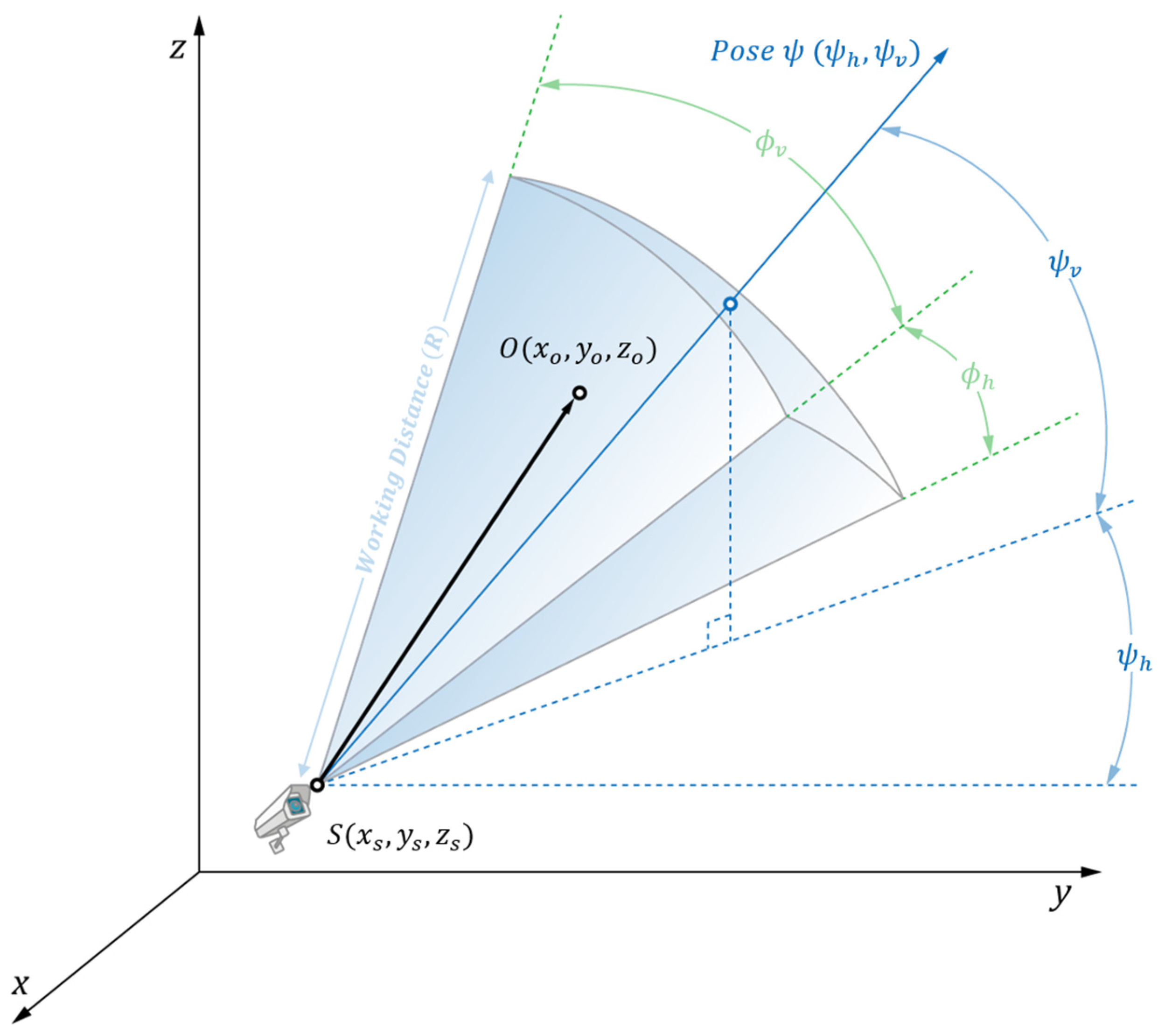
FoV is defined as the visible area of a camera, which can be calculated from the horizontal and vertical view angles (), the working distance (R), and the pose (ψ), as shown in Figure 1. The horizontal and vertical camera view angles ( and , respectively) can be specified from the camera specifications. On the other hand, the horizontal and vertical poses ( and , respectively) describe the azimuth and elevation of a camera and they are decision variables. The positions of surveillance targets and cameras are represented by using the Cartesian coordinate system, while the poses and view angles of cameras are represented by using a spherical coordinate system.
As shown in Figure 1, the distance vector () between a camera position S and a given target point O in the monitoring space is:
Based on Equation (1), the following three Equations (2)–(4) must be satisfied for the point to be covered by the FoV of the camera:
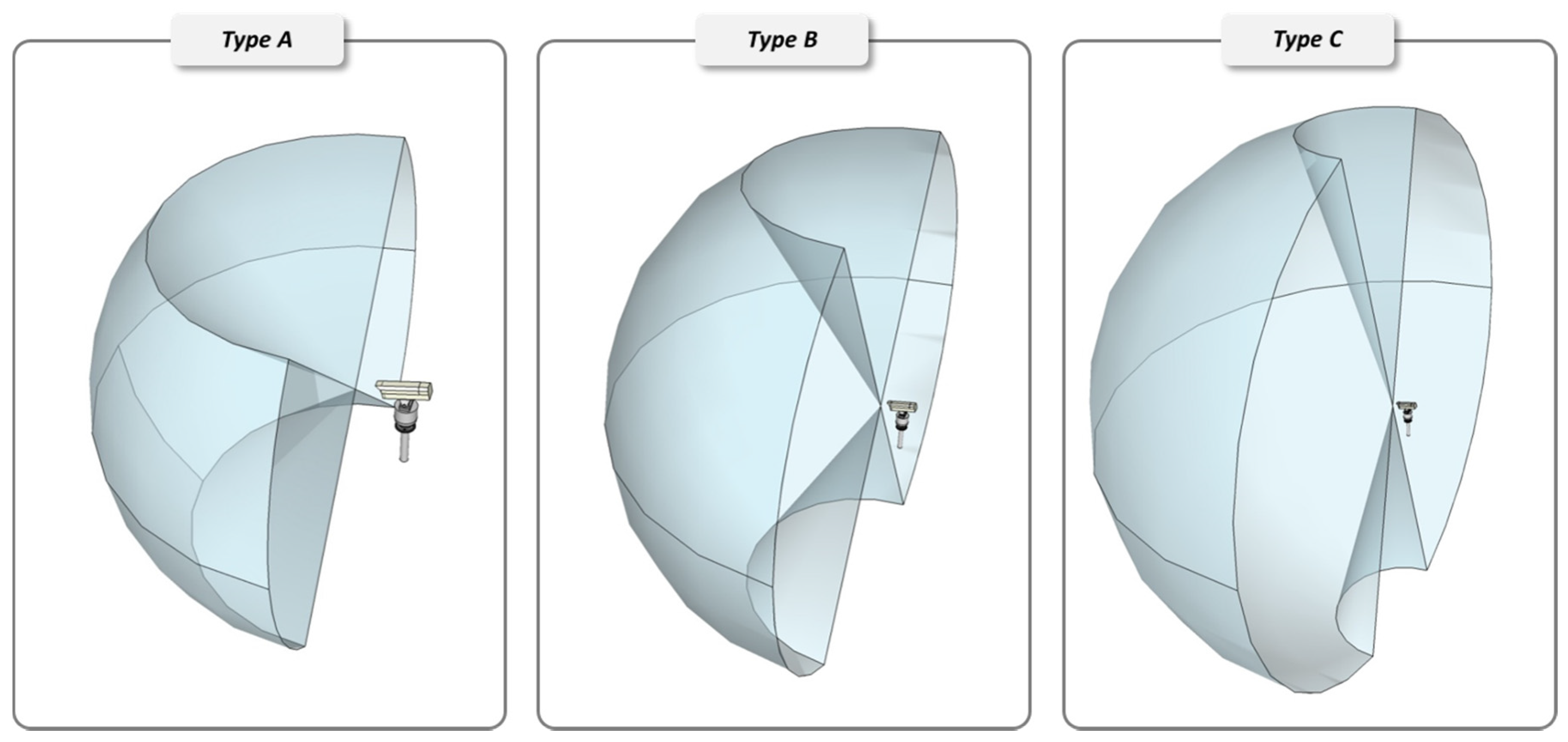
To cover a larger area than that covered by the typical pin-hole cameras and to reduce the number of cameras, we consider PTZ cameras for surveillance applications. A vertical rotation and a horizontal rotation correspond to the tilt and the pan, respectively. To specify the FoV of PTZ cameras while considering pan and tilt, we employ the concept of a reachable region from a previous study [22]. The reachable region of a camera is defined as the intersection of the two regions that the camera can cover in the worst-case scenario. Further, we incorporate zooming into the working distance (R) of a camera, as shown in Figure 2. The detailed specifications of three different PTZ cameras are shown in Table 2.
3.2. Occlusions
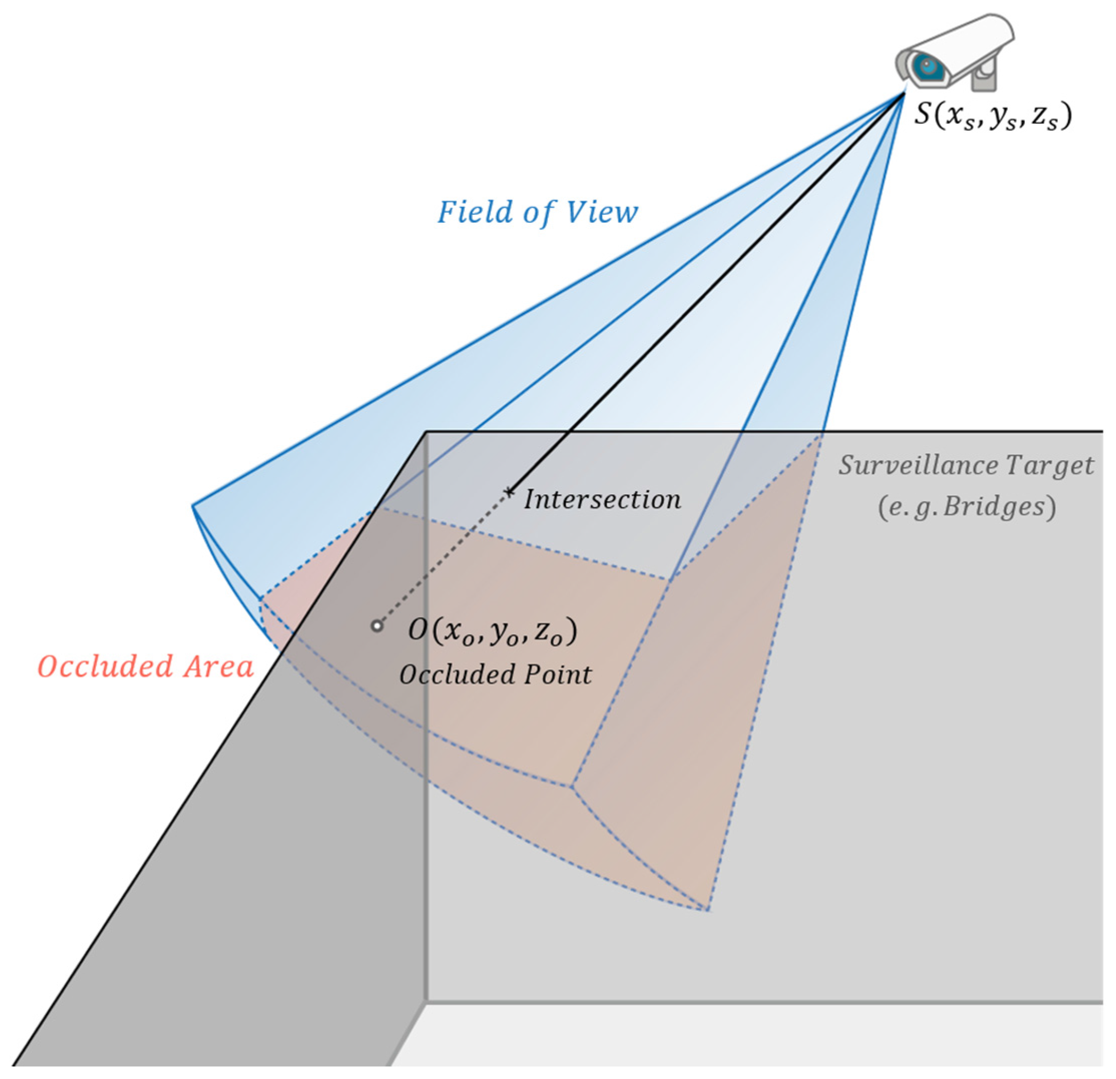
In some situations, cameras may not be able to view the entire FoV owing to occlusions such as the planes of surveillance targets. Figure 3 shows the situation in which the occlusion could interfere with the FoV of a camera. The blue area within the normal FoV of a camera is covered by the camera sensor; the red area represents the invisible area occluded by edges and planes of the grey box. In this study, we regard it as static occlusions, which are known to affect the given cameras in the same manner at any time [23]. The consideration of occlusions is a fundamental step in the development of efficient algorithms considering the actual coverage of the camera because the occluded zone that is not visible from a given camera could be covered by other cameras.
To check whether a target point O is covered, we define the line of sight () between the target point and the camera position S. If there exists an intersection point between the defined line and a plane (as shown in Figure 3), the point is excluded.
3.3. Surveillance Target
The prompt detection of destroyed infrastructure is essential for the creation of an efficient restoration plan after natural disasters. In particular, bridges play an important role in the delivery of supplies to many disaster-struck areas. In many cases, bridges can be modeled as the shape of a long rectangle in 3D space, as shown in Figure 4. Target points for surveillance are located on the surface of the bridge modeled as a rectangle.
However, the placement of cameras in the central area of bridges is highly restricted owing to the rectangular shape of bridges and geographical constraints such as rivers. Therefore, in this study, we address this problem by considering feasible locations for the camera based on the shape of the bridge. The bridge specifications used in the simulation experiments are based on the distribution of height, width, and length from the data of bridges obtained from the national geographic information statistics of the Republic of Korea. Further, in Section 5, we investigate the case study of Samoonjin Bridge to illustrate the camera placement problem and the algorithms for quick planning of bridge restoration.
3.4. Mathematical Modeling
| = | Index of target points | |
| = | Index of potential camera positions | |
| = | Index of camera types | |
| = | Index of possible poses | |
| = | ||
| = | Cost of a camera type k | |
| = | Minimum coverage (%) | |
| = | ||
| = |
The mathematic model for the camera placement problem for minimizing costs while satisfying the minimum coverage level is:
| Minimize | (5) | |
| Subject to | (6) | |
| (7) | ||
| (8) | ||
| (9) | ||
| (10) |
The objective (5) is to minimize the total cost of cameras. Equation (6) represents a target point i to be covered when one or more sensors are located. To ensure that only one camera is assigned to a specific camera position, Equation (7) is added for each camera position. Equation (8) is used to satisfy the minimum level of coverage. Equations (9) and (10) specify the integer requirements for decision variables.
Although optimal solutions can be found using the proposed mathematical model, it is generally difficult to solve reasonable-size camera placement problems within a reasonable time [24]. In the case of camera placement for large structures in 3D space, the number of decision variables, such as and , surges because the number of feasible camera locations and grid points increase given the nature of the NP-hard problem [11,17], and the optimal solution might not be obtained even if it takes an extremely long time. In addition to the increasing number of decision variables, various constraints of the camera placement problem lead to a more accurate result of the problem but increase the computation time for calculating . Furthermore, the size of the problem often exceeds the memory limitation, considering the broader surveillance area and additional camera parameters in 3D space. Therefore, we propose heuristic approaches for the surveillance of large infrastructures in the next section of this study.
4. Proposed Algorithm
The objective of the problem defined in Section 3 is to minimize the total cost of cameras and to determine their optimal placement for the surveillance of bridges such that the minimum coverage level is satisfied. When considering the defined camera placement problem in the real world, the most important challenge is to determine the number of cameras and to assign specific positions and poses for these cameras within a reasonable amount of time. However, considering the complete enumeration of all possible types, positions, and poses of cameras is impractical for most problems owing to their NP-hard nature and the limited size of memory.
To solve the camera placement problem, we propose two algorithms: a genetic algorithm and a uniqueness score with local search algorithm (ULA). These two algorithms include the same process, which is called the visibility test; the visibility test consists of the FoV test and occlusion test. To reduce the calculation time, a visibility matrix consisting of the coverage-point information for all available camera positions and poses is calculated in the initial stage of the proposed algorithms.
4.1. Visibility Test
In theory, cameras can be placed anywhere in 3D space as continuous variables. However, due to the limitations of memory size and computational complexity, an approximation of the surveillance area by 3D grid points is widely used [17]. In this study, we assume that cameras are deployed at discrete grid points. This approach quantizes the search space into many finite candidate placements and searches for the best configurations of combinatorial problems that optimize a given cost function. Cameras are constrained to be placed only at these discrete grid points with the minimum distance between camera grid points equal to ; further, the coverage of cameras is calculated based on grid points with the minimum distance between surveillance target grid points being equal to . Also, the azimuth and elevation are quantized into eight and five equiangular positions to reduce the search space.
The minimum distance between the two grid points corresponding to a surveillance target and a camera is determined by the size of the surveillance area and the requirements related to the computation time and solution quality. If the minimum distance between two grid points decreases, the probability of finding better solutions and the search space of the camera placement problem increase. In addition, to reduce the search space efficiently, we define the minimum level of coverage for each grid point of the camera. If a grid point of the camera does not satisfy the minimum level of coverage, the point is excluded from the visibility matrix. The visibility test consists of two parts: the FoV test and occlusion test. The detailed procedures are described below:
- From geographic information, identify all available camera positions and surveillance regions as grid points.
- Perform the FoV test: Calculate covered points for all available camera positions, types, azimuths, and elevations.
- Perform the occlusion test: Adjust coverage points by considering occlusions for all available camera positions.
- Obtain an adjusted visibility matrix based on the data.
After performing the FoV test and occlusion test, a visibility matrix with camera placements—including possible positions and poses—is generated. In this study, a camera position in the visibility matrix is called a candidate camera placement, which is a combination of four parameters: position in 3D space (S), camera type, azimuth, and elevation. Before finding a solution for the camera placement problem, some of the points covered by a camera in the visibility matrix should be excluded because some planes of surveillance targets can restrict the FoV of cameras. This step is designed to find invisible areas and update the visibility matrix with these occlusions.
4.2. Greedy Algorithm
In the greedy algorithm, camera placements satisfying the minimum covered target grid points are listed and the camera placement with the lowest cost is selected in sequential order. If the greedy algorithm satisfies the minimum coverage level or if it reaches the maximum number of cameras, the algorithm stops and returns the current camera placement. The major advantage of the greedy algorithm is a faster computation time compared to other heuristics.
4.3. Genetic Algorithm
To reduce the computation time, the proposed GA performs the visibility test before the mutation, crossover, and selection loops. The entire genetic algorithm procedure can be described as follows:
- An initial population of N chromosomes is generated by a random algorithm [9] based on the camera placement information, including positions, types, and poses in the visibility matrix.
- For each chromosome of the population, the total cost and coverage level are calculated. The coverage level is calculated as the number of covered grid points of the surveillance target divided by the total number of grid points of the surveillance target.
- A population group that satisfies the minimum level of coverage is selected for reproduction by using the tournament selection method.
- From the population selected in step 3, a new population of the next generation is generated by using crossover and mutation operations.
- 2, 3, and 4 are repeated until the stopping criterion is satisfied.
4.3.1. Chromosome Representation
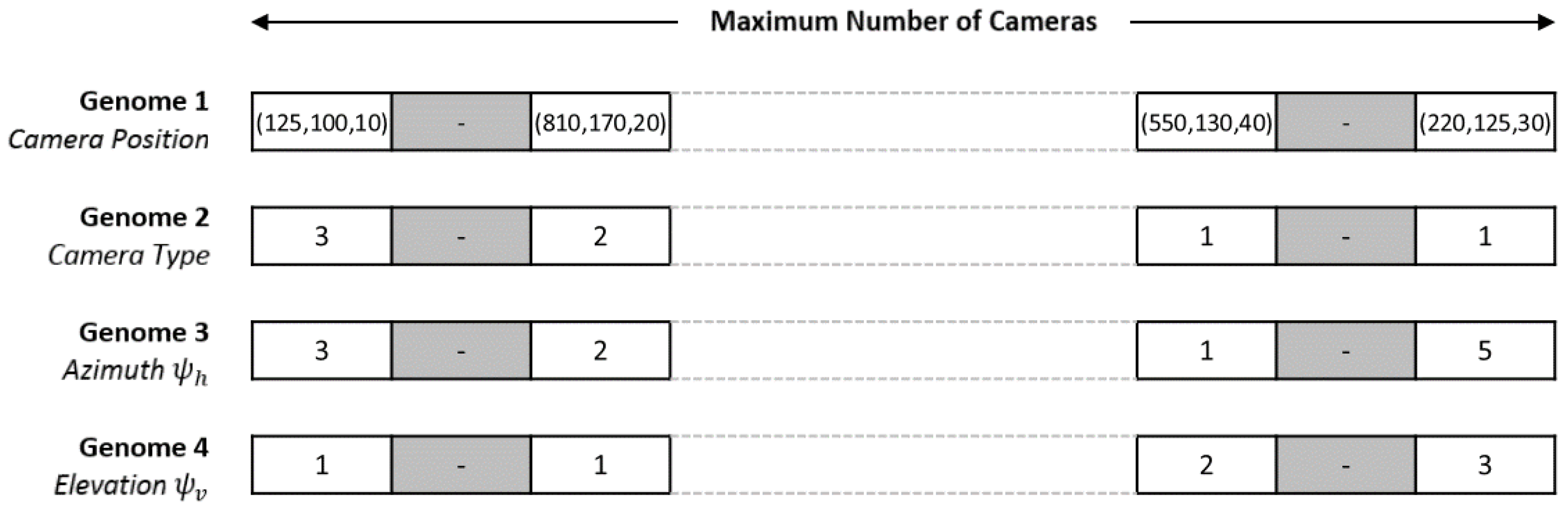
Each chromosome consists of four vectors: camera position, type, azimuth, and elevation vectors, as shown in Figure 5. The length of a chromosome represents the maximum number of cameras. The first vector in a chromosome denotes the camera position (). If there is no camera at a position, the value of the gene is 0. The second vector represents the type of the camera position. The third and fourth vectors represent the azimuth and elevation of the camera, respectively. These two vectors determine the pose of the camera ()). The initial population is generated by selecting camera placements randomly within the maximum number of cameras until the chromosome satisfies the minimum coverage level.
4.3.2. Mutation and Crossover
Mutation and crossover operations can maintain the diversity in a population; further, they enable the genetic algorithm to avoid local minima by preventing solutions from becoming too similar. In order to change the camera position, type, elevation, and azimuth in the selected chromosome, a mutation operator randomly selects a predefined number of genes (mutation parameter m) and reassigns them to another placement in the visibility matrix. Because changes of preassigned camera placements can affect the total coverage, the random reassignment of the predefined number of genes is repeated until the minimum coverage level of the mutated chromosome is guaranteed.
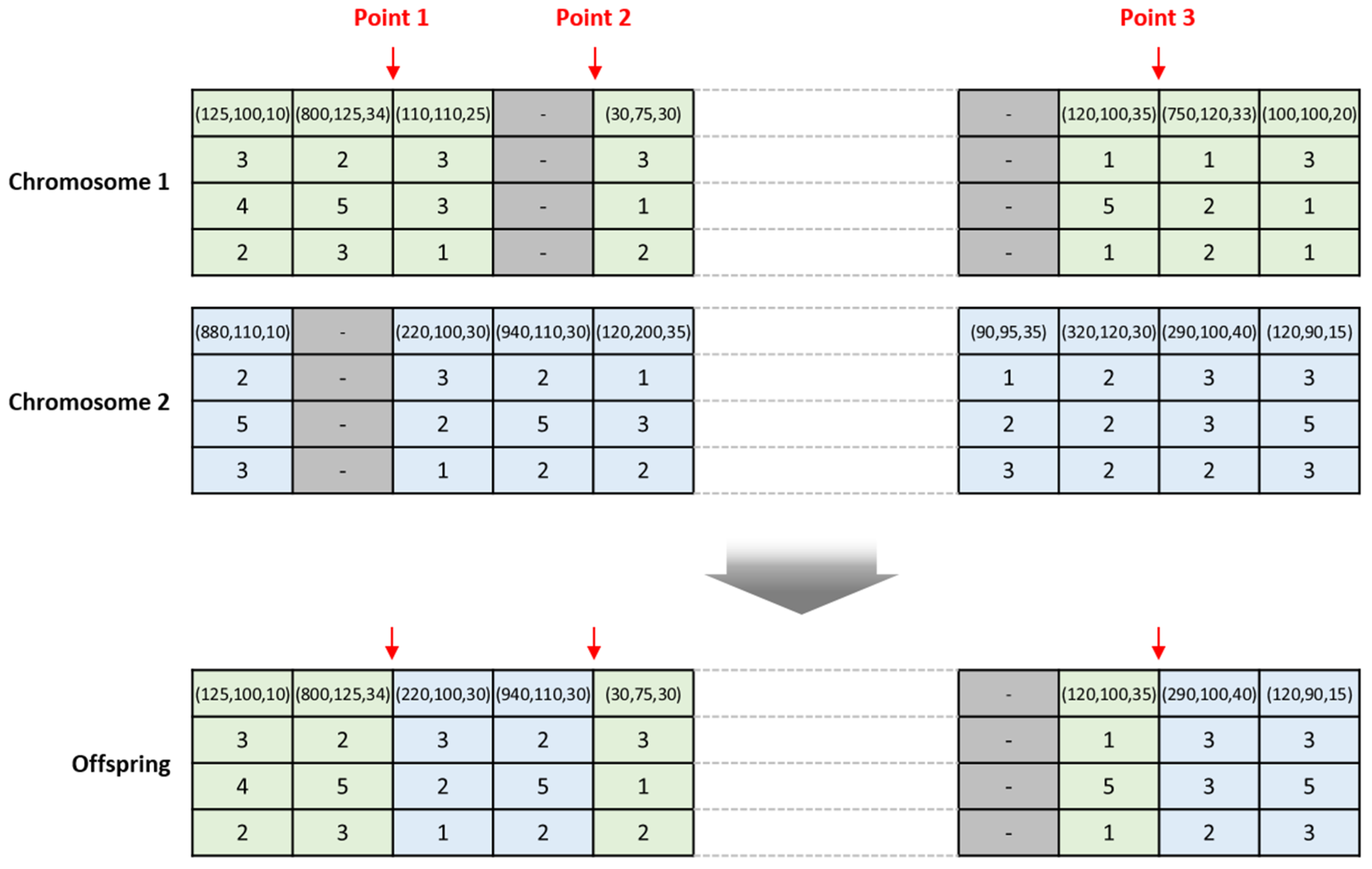
In addition, the three-point crossover operator selects three points randomly, and two parent organism strings between the selected three points are swapped to render an offspring chromosome. Similar to the mutation operator, the entire procedure of the crossover operation is repeated until the offspring chromosome satisfies the minimum coverage. An example of the implementation of the crossover operator is shown in Figure 6.
4.3.3. Selection, Fitness Function, and Stopping Criterion
The next surviving chromosomes are selected using the tournament selection method. The fitness function is the total cost of cameras satisfying the minimum coverage level. The maximum number of generations is employed as a stopping criterion.
4.4. Uniqueness Score with Local Search Algorithm (ULA)
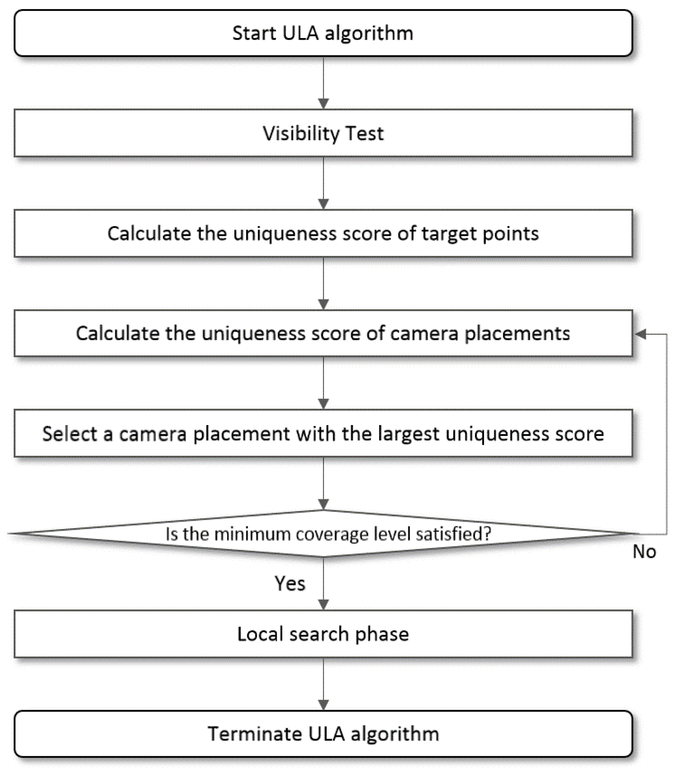
We present a new heuristic algorithm based on the uniqueness score with local search. The flowchart of the proposed algorithm is shown in Figure 7.
4.4.1. Camera Placement with Uniqueness Score
In the proposed ULA algorithm, the seed solution for local search is generated by placing cameras based on their uniqueness scores. If a camera placement has a lower uniqueness score than other camera placements, that placement is characterized as lacking cost-effectiveness because the grid points of the target that are covered by the camera placement tend to be covered by other cameras that have lower costs. The uniqueness score of target points and of a camera placement are defined as follows:
First, the uniqueness of target points () in Equation (11) is calculated for all target points. s and o represent the camera placement in the visibility matrix and the target grid point, respectively. denotes the total number of camera placements s in the visibility matrix. In Equation (12), indicates whether the camera placement s can cover the target point o, which is not covered by selected camera placements in the previous steps. If camera placement s can cover target point o uncovered by the selected camera placements, = 1; otherwise, = 0.
The uniqueness score of the camera placement s is composed of the weighted sum of the uniqueness of target points and . and denote the uniqueness weight and the installation cost of camera placement s, respectively. Camera placements in the visibility matrix are allocated in a non-increasing order of the total uniqueness score (). When a camera placement is selected, the uniqueness scores of the placements of unselected cameras are updated based on the previous results of selection.
4.4.2. Local Search
After finding a solution based on the uniqueness score, the local search algorithm is applied to improve the current solution by determining better solutions at the cost-of-coverage level. The purpose of this algorithm is to cut the total camera cost while satisfying the minimum level of coverage, because the algorithm based on uniqueness scores tends to select expensive cameras that provide higher coverage. In this phase, the applied local search procedure can be described as follows:
- Specify a seed solution and select a camera placement s with the lowest total uniqueness score () in the solution.
- Generate neighborhoods by interchanging s with another camera having a lower cost and then add these neighborhoods to a neighborhood set N.
- Compute the total cost and coverage level of all neighborhoods in N, and then rank the neighborhoods in a non-increasing order of the total cost.
- If the total cost of a neighborhood solution that satisfies the minimum coverage level is lower than the seed solution, update the seed solution with the neighborhood solution. If there is no improvement of cost for any neighborhood, do not update the seed solution.
- Update s with the next lowest and go to step 2. If s is the camera placement with the highest , then return the seed solution.
5. Experimental Result
5.1. Experiment Design
In the simulation experiments, surveillance targets and available positions of cameras were generated based on the real-world bridge data obtained from the Republic of Korea Ministry of Land, Infrastructure and Transport’s 2015 national geographic information statistics. First, we extracted from the data the distribution of the width, height, and length of about 600 bridges. Then, based on the number of target grid points, we divided the bridges into three categories: small, medium, and large. We also generated 40 problem sets for each category, which were used to compare the average performance of the algorithms and identify the feasible camera locations based on the map data. For each problem set, we repeated the simulation experiments for three minimum coverage levels (80%, 85%, and 90%). Table 3 shows the experimental parameters for all the algorithms used in this study.
All the algorithms were coded in C# and were run on a PC with an Intel i5 3.4 GHz processor and 8 GB RAM. In order to evaluate the performance of a probabilistic search method, several pilot experimental tests were conducted to select the best parameter values for GA and we repeated the simulation experiments for different surveillance target sizes.
5.2. Experimental Evaluation
The average total costs, number of cameras, coverages, and computation times of GA, ULA, and greedy algorithm for 40 experiments are compared in Table 4, Table 5 and Table 6. Based on the simulation results, it was obvious that the ULA outperforms the GA and greedy algorithm, because the ULA demonstrates a significantly lower average cost and a lower number of cameras. Furthermore, the ULA’s average coverage is greater than that of the GA and greedy algorithm for the large-sized, medium-sized, and small-sized problems.
In the simulation experiment, as the size of the bridges increased, the performance gap—in terms of the computation time and total cost—between the ULA and other algorithms increased significantly. In addition, as the minimum coverage level increased, the GA’s computation time and total cost were greater than those of the ULA, though neither algorithm’s average computation time changed significantly. In some cases of the greedy algorithm, despite its quick computation time, the total cost increases rapidly as the minimum coverage level increases.
These simulation results showed that the performance of the GA depended mainly on the quality of the initial population generated by the random algorithm, because the initial solution played an important role in determining the eventual outcome. In addition, the greedy algorithm cannot find a good solution when it fails to find camera placements for covering the remaining surveillance areas effectively. Hence, we concluded that the proposed ULA can achieve a better solution than the GA and greedy algorithm can for the same parameters, computation times, and all problem sizes.
5.3. Case Study: Samoonjin Bridge
To illustrate an application of the proposed algorithm, we present a case study of Samoonjin Bridge in Korea with actual data. Before applying the algorithm, we created a 3D model by analyzing the satellite photograph and specifications of the bridge; this 3D model is shown in Figure 8.
The length, width, and height of the bridge are 780 m, 10.9 m, and 13.5 m, respectively. The minimum distances for cameras and target grid points ( and , respectively) are 10 m and 2 m, respectively. The other parameters are set to the same values as in the previous simulation tests (shown in Table 3).
After the visibility test phase, the total number of surveillance target grid points is 7852 and the number of candidate camera placements is 37,963. Based on the result, we applied GA and ULA, which showed a better performance in the previous experiments, to find a solution to the defined camera placement problem; the experimental results are compared in Table 7.
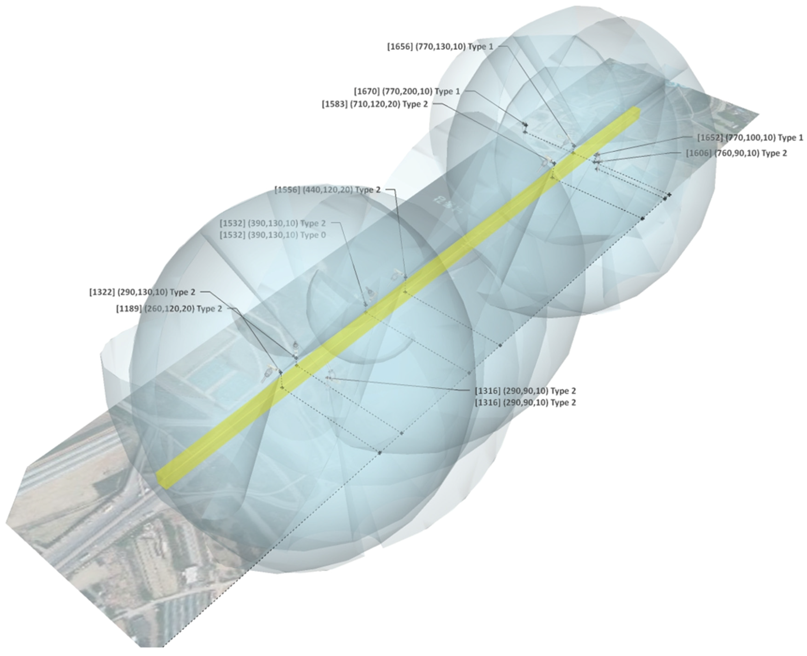
From the results, ULA outperforms GA in terms of cost, coverage, and computation time. The total number of cameras used is 12, and the total cost is approximately USD 108,000. A camera placement using ULA is depicted in Figure 9.
The yellow region represents the simplified 3D model of Samoonjin Bridge, and the blue regions are the visualization of the FoV of the cameras. We observe that the cameras covering the central area of the bridge form a major portion of the covered target grid points owing to the geographical characteristics of the bridge.
6. Conclusions and Future Work
In this study, we first defined the assumptions and constraints of the camera placement problem for the surveillance of bridges. The objective of the defined problem is to minimize the total cost of cameras. To solve the problem within a reasonable amount of time, we proposed a greedy algorithm and GA with the visibility test to explore possible solutions effectively. We also developed a heuristic algorithm called ULA that incorporates the concepts of a uniqueness score and local search. Simulation results demonstrate that ULA outperforms the greedy algorithm and GA in terms of the average cost, coverage, and computation time for all problem sizes and minimum coverage levels. Further, we presented a case study of Samoonjin Bridge to illustrate the entire process of ULA.
The main contribution of this study is the development of a heuristic algorithm to efficiently solve the camera placement problem. The increased complexity of the 3D space with the consideration of occlusions has triggered a necessity for the development of efficient algorithms to solve the problem. The proposed ULA’s competitiveness with respect to efficiency and the ability to solve large camera placement problems was verified based on the results of the simulation that used real-world data. In this context, the ULA has numerous applications for various types of surveillance of important infrastructural components, including buildings and roads in addition to bridges. In addition, because of its ability to find a good solution quickly, the proposed algorithm can be used to consider changes in the environment. For example, various environments, such as budget levels and occluded points caused by dynamic obstacles, can be altered from time to time. Thus, a sensitivity analysis is helpful in considering these changes, and a quicker computation time is crucial in order to find a good solution in a variety of scenarios.
Nevertheless, the proposed approach has some limitations. First, because the proposed algorithm was based on a local search algorithm, it can converge to local optima. Second, the study did not consider mathematical approximation techniques for the camera placement problem.
Future work could pursue several directions. First, the proposed algorithm can be applied to various objectives, including multi-objective optimization problems in which the objective function combines cost and coverage. In this case, by exploiting the proposed algorithm with a quick computation time, we can find Pareto frontiers for multi-objective optimization problems in various scenarios. Furthermore, in terms of dynamic objects, the use of drones with a camera may offer opportunities to expand the applications of the proposed algorithm. In addition, approaches for reducing the decision variables of mathematical models, the parameters, and the constraints and linear relaxations are all worthy of further investigation to verify the performance of the proposed algorithm more exhaustively. Finally, it is worthwhile to assess improving the ULA further to avoid converging to local optima.
Acknowledgments
This research was supported by a grant (17SCIP-B065985-05) from Smart Civil Infrastructure Research Program funded by Ministry of Land, Infrastructure and Transport (MOLIT) of Korea government and Korea Agency for Infrastructure Technology Advancement (KAIA).
Author Contributions
Sungbum Jun and Tai-Woo Chang conceived and designed the algorithms, especially Sungbum Jun, who proposed the ULA; Sungbum Jun and Tai-Woo Chang analyzed the data; Sungbum Jun, Tai-Woo Chang, and Hyuk-Jin Yoon wrote the paper.
Conflicts of Interest
The authors declare no conflict of interest.
References
- Cole, R.; Sharir, M. Visibility problems for polyhedral terrains. J. Symb. Comput. 1989, 7, 11–30. [Google Scholar] [CrossRef]
- Hörster, E.; Lienhart, R. On the optimal placement of multiple visual sensors. In Proceedings of the 4th ACM International Workshop on Video Surveillance and Sensor Networks, Santa Barbara, CA, USA, 27 October 2006; pp. 111–120. [Google Scholar]
- Fleishman, S.; Cohen-Or, D.; Lischinski, D. Automatic camera placement for image-based modeling. In Computer Graphics Forum; Blackwell Publishers: Hoboken, NJ, USA, 2000; Volume 9, pp. 101–110. [Google Scholar]
- Van den Hengel, A.; Hill, R.; Ward, B.; Cichowski, A.; Detmold, H.; Madden, C.; Dick, A.; Bastian, J. Automatic camera placement for large scale surveillance networks. In Proceedings of the 2009 Workshop on Applications of Computer Vision (WACV), Snowbird, UT, USA, 7–9 December 2009; pp. 1–6. [Google Scholar]
- O’rourke, J. Art Gallery Theorems and Algorithms; Oxford University Press: Oxford, UK, 1987; ISBN 0-19-503965-3. [Google Scholar]
- Marengoni, M.; Draper, B.A.; Hanson, A.; Sitaraman, R. A system to place observers on a polyhedral terrain in polynomial time. Image Vis. Comput. 2000, 18, 773–780. [Google Scholar] [CrossRef]
- Zhou, P.; Long, C. Optimal coverage of camera networks using PSO algorithm. In Proceedings of the 2011 4th International Congress on Image and Signal Processing (CISP), Shanghai, China, 15–17 October 2011; Volume 4, pp. 2084–2088. [Google Scholar]
- Yabuta, K.; Kitazawa, H. Optimum camera placement considering camera specification for security monitoring. In Proceedings of the IEEE International Symposium on Circuits and Systems (ISCAS 2008), Seattle, WA, USA, 18–21 May 2008; pp. 2114–2117. [Google Scholar]
- Jiang, Y.; Yao, X.; Wang, W.; Gu, L. New method for weighted coverage optimization of occlusion-free surveillance in wireless multimedia sensor network. In Proceedings of the 2010 First International Conference on Networking and Distributed Computing (ICNDC), Hangzhou, China, 21–24 October 2010; pp. 31–35. [Google Scholar]
- Belhaj, L.A.; Gosselin, S.; Pouyllau, H.; Semet, Y. Smart-sensor placement optimization under energy objectives. In Proceedings of the 2016 Global Information Infrastructure and Networking Symposium (GIIS), Porto, Portugal, 19–21 October 2016; pp. 1–7. [Google Scholar]
- Gupta, A.; Pati, K.A.; Subramanian, V.K. A NSGA-II based approach for camera placement problem in large scale surveillance application. In Proceedings of the 2012 4th International Conference on Intelligent and Advanced Systems (ICIAS), Kuala Lumpur, Malaysia, 12–14 June 2012; Volume 1, pp. 347–352. [Google Scholar]
- Ma, H.; Zhang, X.; Ming, A. A coverage-enhancing method for 3D directional sensor networks. In Proceedings of the INFOCOM 2009, Rio de Janeiro, Brazil, 19–25 April 2009; pp. 2791–2795. [Google Scholar]
- Murray, A.T.; Kim, K.; Davis, J.W.; Machiraju, R.; Parent, R. Coverage optimization to support security monitoring. Comput. Environ. Urban Syst. 2007, 31, 133–147. [Google Scholar] [CrossRef]
- Burelli, P.; Yannakakis, G.N. Global search for occlusion minimisation in virtual camera control. In Proceedings of the 2010 IEEE Congress on Evolutionary Computation (CEC), Barcelona, Spain, 18–23 July 2010; pp. 1–8. [Google Scholar]
- Jun, S.; Chang, T.-W.; Jeong, H.; Lee, S. Camera Placement in Smart Cities for Maximizing Weighted Coverage with Budget Limit. IEEE Sens. J. 2017, 17, 7694–7703. [Google Scholar] [CrossRef]
- Ghanem, B.; Cao, Y.; Wonka, P. Designing camera networks by convex quadratic programming. Comput. Graph. Forum 2015, 34, 69–80. [Google Scholar] [CrossRef]
- Morsly, Y.; Aouf, N.; Djouadi, M.S.; Richardson, M. Particle swarm optimization inspired probability algorithm for optimal camera network placement. IEEE Sens. J. 2012, 12, 1402–1412. [Google Scholar] [CrossRef]
- Mavrinac, A.; Chen, X. Modeling coverage in camera networks: A survey. Int. J. Comput. Vis. 2013, 101, 205–226. [Google Scholar] [CrossRef]
- Indu, S.; Chaudhury, S.; Mittal, N.R.; Bhattacharyya, A. Optimal sensor placement for surveillance of large spaces. In Proceedings of the 3rd ACM/IEEE International Conference on Distributed Smart Cameras (ICDSC 2009), Como, Italy, 30 August–2 September 2009; pp. 1–8. [Google Scholar]
- Piciarelli, C.; Micheloni, C.; Foresti, G.L. Occlusion-aware multiple camera reconfiguration. In Proceedings of the 4th ACM/IEEE International Conference on Distributed Smart Cameras, Atlanta, GA, USA, 31 August–4 September 2010; pp. 88–94. [Google Scholar]
- Ding, C.; Song, B.; Morye, A.; Farrell, J.A.; Roy-Chowdhury, A.K. Collaborative sensing in a distributed PTZ camera network. IEEE Trans. Image Process. 2012, 21, 3282–3295. [Google Scholar] [CrossRef] [PubMed]
- Erdem, U.M.; Sclaroff, S. Automated camera layout to satisfy task-specific and floor plan-specific coverage requirements. Comput. Vis. Image Underst. 2006, 103, 156–169. [Google Scholar] [CrossRef]
- Hanel, M.L.; Kuhn, S.; Henrich, D.; Grüne, L.; Pannek, J.R. Optimal camera placement to measure distances regarding static and dynamic obstacles. Int. J. Sens. Netw. 2012, 12, 25–36. [Google Scholar] [CrossRef]
- Zhao, J.; Yoshida, R.; Cheung, S.C.S.; Haws, D. Approximate techniques in solving optimal camera placement problems. Int. J. Distrib. Sens. Netw. 2013, 9, 241913. [Google Scholar] [CrossRef]
Figure 1.
Field of view (FoV) of camera.

Figure 2.
FoV of three pan-tilt-zoom (PTZ) cameras.

Figure 3.
Occlusion of camera. Occluded points in the visibility matrix should be excluded because some planes of surveillance targets can restrict the FoV of cameras.
Figure 3.
Occlusion of camera. Occluded points in the visibility matrix should be excluded because some planes of surveillance targets can restrict the FoV of cameras.

Figure 4.
3D modeling of surveillance target.
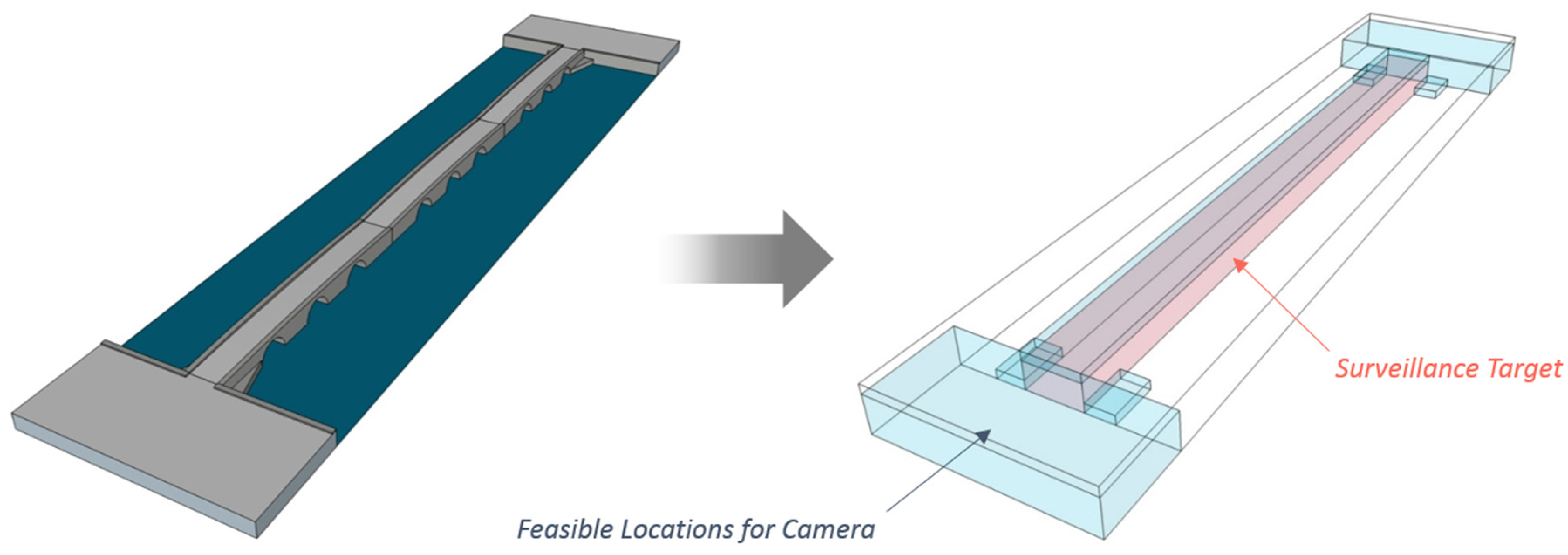
Figure 5.
Chromosome representation. A chromosome has four vectors: 3-D camera position, camera type, azimuth, and elevation.
Figure 5.
Chromosome representation. A chromosome has four vectors: 3-D camera position, camera type, azimuth, and elevation.

Figure 6.
Three-point crossover operator.

Figure 7.
Overall local search algorithm (ULA) framework.

Figure 8.
3D model of Samoonjin Bridge. The blue area represents feasible locations for the camera and Samoonjin Bridge is modeled as the yellow area.
Figure 8.
3D model of Samoonjin Bridge. The blue area represents feasible locations for the camera and Samoonjin Bridge is modeled as the yellow area.
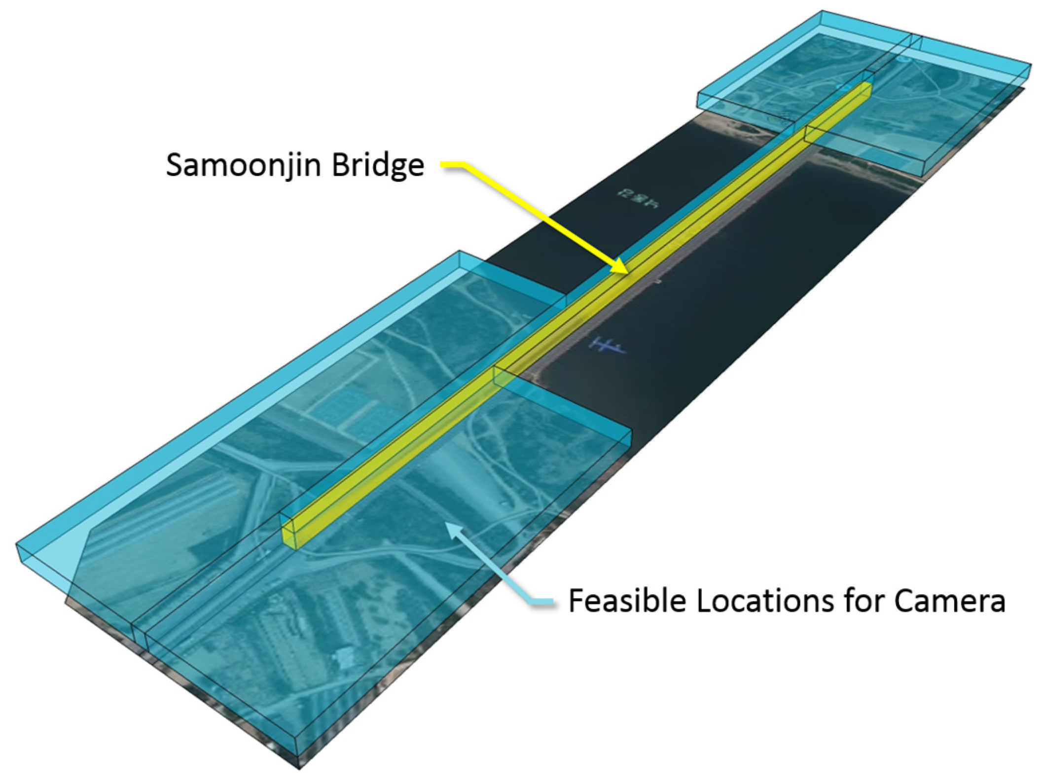
Figure 9.
Illustration of a camera placement using ULA. The blue spheres represent FoV of PTZ cameras.
Figure 9.
Illustration of a camera placement using ULA. The blue spheres represent FoV of PTZ cameras.

Table 1.
Summary of previous literature about the camera placement problem.
| Space | Objective | Solution Approach | Reference |
|---|---|---|---|
| 2D | Max. Coverage | Particle swarm optimization (PSO) | [7] |
| Max. Coverage, Min. Cost | Greedy algorithm and Dual sampling algorithm | [2] | |
| Max. Weighted Coverage | Binary integer programming (BIP) | [8] | |
| Genetic algorithm, Self-orientation algorithm, and Random algorithm | [9] | ||
| Multi-Objective (Min. Cost, Min. Motion, and Min. Maximum Brightness) | Covariance matrix adaptation-evolution strategy (CMA-ES) | [10] | |
| Multi-Objective (Max. Effective Coverage, Min. Cost, and Max. Total Visibility) | Non-dominated sorting Genetic algorithm (NSGA-II) | [11] | |
| 3D | Max. Coverage | Greedy algorithm based on an Image-based model | [3] |
| Simulated annealing (SA)-based area coverage enhancing algorithm | [12] | ||
| Max. Weighted Coverage | Binary integer programming (BIP) | [13] | |
| Genetic algorithm, Octree-based search, and Random search | [14] | ||
| Collaboration-based local search algorithm (COLSA) | [15] | ||
| Max. Weighted Coverage, Min. Number of Camera | Binary quadratic programming (BQP) | [16] | |
| Min. Cost | Particle swarm optimization (PSO) | [17] |
Table 2.
Specifications of three PTZ cameras: A, B, and C.
| Camera Types | A | B | C |
|---|---|---|---|
| Vertical reachable region () | [−45°, 45°] | [−60°, 60°] | [−75°, 75°] |
| Horizontal reachable region () | [−90°, 90°] | [−90°, 90°] | [−90°, 90°] |
| Working distance with zooming (R) (meter) | 60 | 120 | 180 |
| Estimated cost (USD) | 4000 | 8000 | 10,000 |
Table 3.
Experimental parameters. GA: genetic algorithm; ULA: local search algorithm.
| Parameters | Values | |
|---|---|---|
| Visibility test | Minimum covered target grid points | 90 |
| Camera grid width () (meter) | 10 | |
| Target grid width () (meter) | 5 | |
| Maximum size of 3D space (meter) | (1000, 220, 50) | |
| GA | Mutation rate | 0.1 |
| Crossover rate | 0.8 | |
| Tournament rate | 0.7 | |
| Maximum number of cameras | 200 | |
| Number of generations | 200 | |
| Number of population | 500 | |
| ULA | Uniqueness weight () | 1 |
| Distribution of bridges | Length (meter) | N(688, 652) |
| Width (meter) | N(14, 52) | |
| Height (meter) | N(21.3, 52) | |
Table 4.
Results summary (Minimum coverage 80%).
| Result types | Small | Medium | Large | ||||||
|---|---|---|---|---|---|---|---|---|---|
| Greedy | GA | ULA | Greedy | GA | ULA | Greedy | GA | ULA | |
| Avg. Computation Time (min) | 0.07 | 5.81 | 3.40 | 0.17 | 8.09 | 5.20 | 0.29 | 9.88 | 6.66 |
| Avg. Number of Cameras | 12.88 | 9.50 | 8.15 | 14.05 | 9.78 | 8.38 | 14.93 | 11.20 | 9.15 |
| Avg. Total Cost (1000 USD) | 104.20 | 90.95 | 80.00 | 113.00 | 94.05 | 81.65 | 119.70 | 105.90 | 88.70 |
| Avg. Coverage (%) | 82.50 | 80.63 | 80.98 | 82.10 | 80.64 | 80.97 | 82.00 | 80.57 | 80.56 |
Table 5.
Results summary (Minimum coverage 85%).
| Result types | Small | Medium | Large | ||||||
|---|---|---|---|---|---|---|---|---|---|
| Greedy | GA | ULA | Greedy | GA | ULA | Greedy | GA | ULA | |
| Avg. Computation Time (min) | 0.09 | 5.88 | 3.38 | 0.21 | 8.14 | 5.21 | 0.33 | 10.00 | 6.65 |
| Avg. Number of Cameras | 14.75 | 10.50 | 9.00 | 16.20 | 11.10 | 9.18 | 17.1 | 12.55 | 10.30 |
| Avg. Total Cost (1000 USD) | 119.90 | 100.90 | 87.65 | 131.00 | 105.90 | 88.65 | 137.9 | 118.10 | 99.50 |
| Avg. Coverage (%) | 86.90 | 85.74 | 85.70 | 87.00 | 85.48 | 85.63 | 86.70 | 85.39 | 85.61 |
Table 6.
Results summary (Minimum coverage 90%).
| Result types | Small | Medium | Large | ||||||
|---|---|---|---|---|---|---|---|---|---|
| Greedy | GA | ULA | Greedy | GA | ULA | Greedy | GA | ULA | |
| Avg. Computation Time (min) | 0.10 | 6.06 | 3.41 | 0.26 | 8.56 | 5.23 | 0.42 | 10.21 | 6.71 |
| Avg. Number of Cameras | 17.70 | 15.55 | 10.58 | 19.03 | 16.48 | 10.78 | 20.45 | 16.60 | 11.75 |
| Avg. Total Cost (1000 USD) | 145.10 | 150.15 | 101.80 | 155.00 | 155.60 | 102.70 | 165.90 | 156.70 | 112.50 |
| Avg. Coverage (%) | 91.40 | 90.19 | 90.81 | 91.10 | 90.12 | 90.39 | 91.30 | 90.20 | 90.29 |
Table 7.
Results summary of Samoonjin Bridge (Minimum coverage 80%).
| Result types | GA | ULA |
|---|---|---|
| Computation Time (min) | 25.15 | 17.42 |
| Number of Cameras | 14 | 12 |
| Total Cost (1000 USD) | 134 | 108 |
| Coverage (%) | 80.15 | 80.07 |
© 2018 by the authors. Licensee MDPI, Basel, Switzerland. This article is an open access article distributed under the terms and conditions of the Creative Commons Attribution (CC BY) license (http://creativecommons.org/licenses/by/4.0/).
Share and Cite
MDPI and ACS Style
Jun, S.; Chang, T.-W.; Yoon, H.-J. Placing Visual Sensors Using Heuristic Algorithms for Bridge Surveillance. Appl. Sci. 2018, 8, 70. https://doi.org/10.3390/app8010070
AMA Style
Jun S, Chang T-W, Yoon H-J. Placing Visual Sensors Using Heuristic Algorithms for Bridge Surveillance. Applied Sciences. 2018; 8(1):70. https://doi.org/10.3390/app8010070
Chicago/Turabian StyleJun, Sungbum, Tai-Woo Chang, and Hyuk-Jin Yoon. 2018. "Placing Visual Sensors Using Heuristic Algorithms for Bridge Surveillance" Applied Sciences 8, no. 1: 70. https://doi.org/10.3390/app8010070
Note that from the first issue of 2016, this journal uses article numbers instead of page numbers. See further details here.