Rule Based Coordinated Control of Domestic Combined Micro-CHP and Energy Storage System for Optimal Daily Cost


1
Department of Electrical Engineering, Northeast Electric Power University, Jilin 132012, China
2
China Electric Power Research Institute, Beijing 100192, China
3
Beijing Key Laboratory of Demand Side Multi-Energy Carriers Optimization and Interaction Technique, Beijing 100192, China
*
Author to whom correspondence should be addressed.
Appl. Sci. 2018, 8(1), 8; https://doi.org/10.3390/app8010008
Submission received: 17 November 2017
/
Revised: 16 December 2017
/
Accepted: 19 December 2017
/
Published: 22 December 2017
(This article belongs to the Special Issue Developing and Implementing Smart Grids: Novel Technologies, Techniques and Models)
Abstract
:This paper presents a novel control algorithm for optimising operational costs of a combined domestic micro-CHP (combined heat and power), battery and heat storage system. Using a minute by minute basic time-step, this work proposes a simple and computationally efficient rule based whole-system management, developed from empirical study of realistic simulated domestic electricity and heat loads. The CHP availability is considered in two binary states which, together with leveraging storage effectively, maximises CHP efficiency, and gives the algorithm increased real world feasibility. In addition, a novel application of a dual battery system is proposed to support the micro-CHP with each battery supplying just one of the distinctive morning and evening electrical load peaks, and thus inherently improving overall battery system lifetime. A case study is presented where the algorithm is shown to yield approximately 23% energy cost savings above the base case, almost 3% higher savings than that of the closest previous work, and 96.8% of the theoretical minimum cost. In general, the algorithm is shown to always yield better than 88% of the theoretical minimum cost, a ratio that will be considerably higher when real-world CHP limitations are factored into the theoretical minimum calculation.
1. Introduction
Recently, large industrial and commercial customers have begun to participate in Smart Grid (SG) programs, for example, demand side management (DSM) and demand response (DR), to save energy costs and reduce CO2 emissions. However, the domestic sector has shown less interest in SG technologies, because of their individually smaller impact on the grid and the technical difficulties in aggregating large numbers of customers [1,2].
However, as reported by the U.S. Department of Energy, buildings consume more energy compared with other broad sectors of energy consumption, such as industry and transportation, approximately 40% compared to 30% each respectively [3]. Since domestic buildings are a very significant share of total buildings, households are responsible for a large proportion of CO2 emissions, through end use of both electricity and gas (or other fossil fuel) [4]. It is therefore urgent to develop cost-effective and practical methods to control energy consumption in residential dwellings.
In order to meet emission reduction targets, renewable energy has been deployed in an increasingly localised and decentralised manner, in the form of distributed generation (DG) [5]. Distributed generation has the added advantage of increasing system robustness and reducing transmission losses [6]. At building level, this takes the form of micro-generation, reducing the reliance on the grid. Energy independence can be increased still further with appropriate energy storage at building level so that local renewably generated energy can be stored until it is required, which increases the self-consumption of renewably generated energy [7,8,9]. Moreover, with increasing uptake of SG technologies (especially smart meter technology), electrical power in buildings can be consumed more efficiently compared with conventional buildings, through change in user behaviour and automation of building services, such as lighting and heating [10,11]. These technologies play important roles to optimise electricity consumption at building level; however they have less impact on other forms of energy use, such as gas space heating and domestic hot water.
Researchers have therefore recently begun to focus on synergies between various kinds of energy carriers such that a holistic treatment can minimise the total overall energy use. In this context, a concept called ‘Energy Hub’ (EH) was proposed to model various forms of energy transformation, conversion and storage considered holistically in a single entity [12]. By integrating different energy carriers, the EH model increases internal and external types of dependencies among different energy carriers. For a multi-energy system, internal dependency is managed by the system operator through applying control strategies to the infrastructures, while external dependency is due to the choice of the energy supply according to customer preferences [13]. Due to the fact that the EH model can improve the dependencies of multi-energy system, it is widely used in recent literature to model the aforementioned technologies in a domestic setting and thus solve household energy optimisation problems.
A comparison of two different heat storage systems is proposed in [14] to analyse the technology and cost of heat storage systems for residential micro-CHP. In [15], an application of multi-agent systems for cyber-enabled energy management of building structures (CEBEMS) is investigated; the CEBEMS models the building cooling, heat and power zones and finally energy zones, coordinates local generation to optimise building energy usage. In [16], the Monte Carlo valuation method for Energy Hubs is proposed. Together with DSM, this method solves the system uncertainty problem and improves system flexibility. However, in [14,15,16], system scheduling and optimisation are only based on heat demand, and electricity demand is neglected.
A multi-time scale structure rule is built to optimise a micro-grid energy system in [17]. It is also claimed that rule based optimisations for energy systems are preferable to algorithm-based optimisations, because they are computationally more efficient and easier to implement in real-world applications in [17]. The types and capacity of DG and storage devices are optimised in [18] using a number of hybridised techniques. By introducing sensitive and non-sensitive load concepts (sensitive loads are those loads in which delivery of power to them should be guaranteed under any conditions.), Moradi, M.H. et al. also develop an operational energy management strategy in micro-grids in [18]. However, in both approaches described in [17,18], the householder’s comfort may be compromised; due to requirements of DR in [17] and considering the non-sensitive load in [18].
In [19], a smart Energy Hub is modelled and multi-energy networks based on an integrated demand side management technique are proposed. Similar to [20,21], the simulation time period for this work is one hour, which does not sufficiently consider dynamic changes of the EH modelled at domestic level.
For integrated energy systems, a combined heat and power (CHP) unit can be used to couple the heat and electricity carriers. Residential buildings can benefit from micro-CHP to simultaneously generate heat and power, and thus provide energy services at increased overall efficiency. Based on [22], the overall capacity for micro-CHP is normally below 15 kW. In some work, for example [4,19], the heat efficiency and electricity efficiency of CHP are assumed to be constant. However, since the output of most micro-CHP may be varied, the efficiency also varies with any dynamic operation. Additionally, a CHP system requires some ramp up time to reach a steady state after it switched on or to match actual output after a set point is changed [23]. Finally, micro-CHP presents the problem of whether to best schedule the output to meet electricity demand, heat demand or a compromise between the two, a problem addressed in this paper with the control rules and the energy storage.
In most work on building level Energy Hub optimisation, instead of attempting to predict load, it is assumed systems have perfect forecasts and so know energy demand in advance [2,4]. However, load prediction at building and micro-grid level can require long computation times and often performs poorly (an average error of 4.8% is given in [24] based on a number studies including [25,26,27]). Alternatively, in [28], a stochastic optimal strategy is proposed to solve the uncertainty of demands. This method can offer more accurate simulation results, however it increases the complexity of computation. It is therefore important to include improved load prediction in future work and always take into account its performance and computation time in the context of overall optimisation.
In this paper, a rule based system optimisation model will be proposed. Moreover, considering the difficulties to precisely predict heat and electricity load at building level, this paper proposes a ‘CHP switch’ (CHPS) algorithm to control energy generation. This algorithm simultaneously considers the heat load and electricity load, which reduces the errors caused by energy prediction. The system time step is set as one minute, and thus will better track the true dynamic changes of the hybrid energy system. The optimisation model presented here further reduces energy cost, by 22.9% compared with 20% in [10].
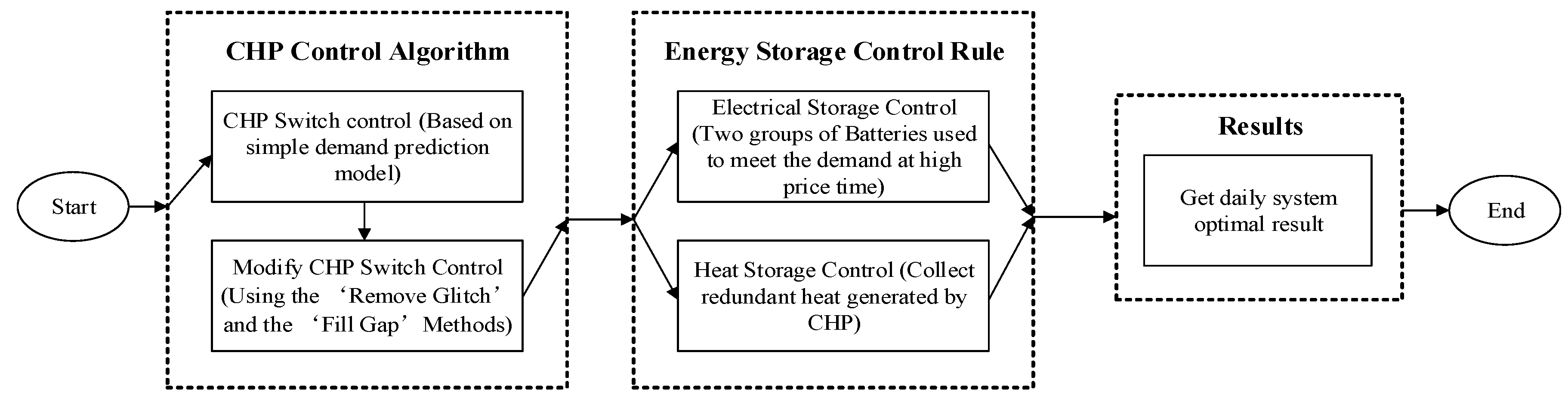
The major contributions of this paper are: (1) developing the rule based control method; (2) constructing a ‘CHP switch’ algorithm; (3) introducing dual battery operation in this context and (4) demonstrating the efficacy of the overall control strategy against a theoretical minimum. The overall optimisation algorithm for the Energy Hub at building level proposed in this paper is summarised in Figure 1.
The rest of this paper is organised as follows. In Section 2, the EH model, CHPS algorithm and modified CHPS algorithm are introduced. In addition, the heat and electrical storage system (HESS) control rule is proposed. Moreover, a method is introduced to calculate theoretical daily minimum operation cost. In Section 3, a case study is used to examine the proposed models and rules. Optimisation results will be compared with theoretical daily minimum operation cost in Section 4. Finally, this paper is concluded in Section 5.
2. Optimisation Methods and Modelling
2.1. The Energy Hub (EH) Model
An Energy Hub is a conceptual model of any bounded area’s energy infrastructure, where different forms of energy can be converted, transmitted and stored [29]. It connects inputs and outputs of multiple energy carriers. Figure 2 gives an example of an Energy Hub.
There are two common ways to establish a matrices equation for an Energy Hub. The first one uses forward-coupling matrices to determine for a set of given inputs, how the dispatch factors and conversion efficiencies determine system outputs [30]. In this way, an Energy Hub model can be mathematically expressed as:
where C represents the coupling matrix. Normally the terms in this matrix are the product of the energy converters efficiencies and the dispatch factor that denotes the proportion of energy flowing into the converter. and are the different energy carrier outputs and inputs power matrix in an Energy Hub respectively. is an equivalent storage power exchange vector. S and represent the storage coupling matrix and steady-state energy storage vector respectively.
However, in order to reduce energy consumption, it is often a requirement to get the minimum input power for a given output power (demand) [31,32]. Therefore, in this way, the EH model can be mathematically where the supplies are explicitly expressed in terms of the loads:
In Equation (2), D represents the backwards coupling matrix. Energy Hubs can be modelled in either way, and both approaches are effective in optimising energy consumption. For a house holder, the daily energy cost optimisation problem can then be formulated as:
where F(x) is a scalar-valued objective function, g(x) normally comes from the conservation of power and h(x) normally comes from limitations, e.g., maximum output power, or number of converters.
To optimise the Energy Hub model, it is important to predict the demands (heat and electricity) precisely, because the predicted demands can be used to inform on control of energy generation systems and energy storage system over a considered time horizon. In Section 2, part 2, short term prediction will be introduced to control power generation system (CHP system control) and in Section 2, part 3, long term prediction will be used to control the energy storage system.
2.2. CHP Switch (CHPS) Algorithm
As mentioned in the Introduction, energy prediction at building level has an average error of approximately 5% [24] whilst short-term prediction level has worse performance. This suggests that a more precise model should be proposed to control the power generation system (CHP system).
Close study of household electrical demand has revealed that it usually changes rapidly and after changing will remain in the same state for several minutes or longer. However, the heating demand fluctuates more smoothly and on slower time scales. After careful study of these two time series, in [33] it was found that the electricity consumption and heat consumption in every minute can be effectively predicted with the following simple equations:
In Equations (6) and (7), and represent the predicted electricity demand and heat demand in (n + 1)th minute, respectively. is the electricity consumption in the nth minute and is the heat consumption in ith minute. In order to evaluate the accuracy of this load prediction approach, more than a hundred sets of daily load time series were tested. This data showed that on a minute by minute base 90.5% of the time the electrical demand is identical to the previous minute.
Clearly there will be some errors between the predicted demands and actual demands by using Equations (6) and (7). This is shown in [33]. However, this has very small influence if heat and electricity generation are considered together. Moreover, the main novelty of [33] is that this paper treats the predicted demands as a reference input just to control the CHP binary switch, whereas other studies, using more sophisticated statistical methods to predict demand, must deal with the whole system’s optimisation. Used specifically to control the switching of CHP, Equations (6) and (7) yield a very low error rate of 3% in terms of time dimension, and have vastly reduced computation times and complexity compared to statistical methods.
After calculating the predicted demands, the benefit that CHP will give in the next minute can be expressed as:
In Equation (8), is the benefit, in monetary terms that CHP can generate at the next minute if it is switched ‘on’. and are the effective value of heat and electrical power contribution due to CHP. and represent the gas and electricity prices. is gas to heat transfer efficiency. The cost to implement CHP in the next minute can be written as:
where is the energy cost of CHP working at the state of rated power and represents the rated power (including heat power, electrical power and losses) of the CHP system. By comparing with the benefit that CHP can generate and the energy cost of CHP working at the state of rated power, the state of CHP can be decided.
This algorithm significantly reduces the error introduced by energy prediction, because it uses the predicted heat demand and electricity demand together to control the ‘CHP switch’. The heat output of CHP is normally much greater than the electricity output (two to four times higher), and the errors of heat prediction are relatively small. This will reduce the error of ‘CHP switch’ model to some extent. Additionally, when the capacity of CHP is carefully designed and considering the fact that the domestic electricity price is usually much higher than the domestic gas price, the state of CHP is influenced by the benefit that CHP can yield. As long as the benefit of implementing CHP is greater than the energy cost of CHP working at the state of rated power, CHP will be switched on. This means, the CHP control system does not need to know the exact heat and electricity demand. Instead, it only needs to know whether the benefit of implementing CHP is greater than the cost, which further reduces the errors introduced by energy prediction. Finally, the short-term prediction is only used in CHP switch control and not for other parts of the system.
2.3. Modified ‘CHP Switch’ Algorithm
This algorithm offers a new way to control the ‘CHP switch’, however, the result is the state of CHP may be changed very frequently in a short time period. However, as mentioned in the introduction, the state of CHP cannot be changed too frequently due to operational restrictions such as ramp up time. Therefore, a modified ‘CHP switch’ algorithm is proposed in this paper to reduce the switching frequency of CHP. This algorithm ideally requires the load to be recorded for at least a year a beforehand. If this data is not available then the daily load can be approximated using heating degree days and total aggregated energy bills, or the load simulators such as those used in [34].
There are two ways to reduce switching frequency of CHP. The first one is to keep CHP on when it should be off, defined in this paper as ‘Fill Gap’, and the second way is to keep CHP off when it should be on, defined in this paper as ‘Remove Glitch’.
The ‘Fill Gap’ method is normally used when the CHP is switched off in a short time period and the energy price is relatively high. On the contrary, ‘Remove Glitch’ is normally used when the CHP is switched on for a very short time period and the energy price is relatively low. By using both ‘Fill Gap’ and ‘Remove Glitch’, the switching frequency can be reduced, which mitigates the cycling stress on the CHP unit and allows it to reach a steady state with maximum operating efficiency. However, for short periods, the CHP will generate surplus energy in the ‘Fill Gap’ and fail to meet load in the ‘Remove Glitch’ mode. This will decrease the efficiency slightly, but can be mitigated with energy storage, and supplemented by the grid if necessary.
When using ‘Fill Gap’ or ‘Remove Glitch’ to reduce CHP switching frequency, it is necessary to have knowledge of the states of CHP in next few following minutes. To obtain states of the CHP in the next few more minutes, ‘probability of CHP switch on’ at each minute in a day is calculated based on historical data.
To get the ‘probability of CHP switch on’ in a day, four steps are required. First, select all the relevant recorded daily energy consumption data from last year as sampling data i.e., data from the corresponding month of the previous year(s). Second, data that covers unusual events need to be removed from the sampling data (for example, days in which the occupants were absent or there was increased occupancy). When combined with occupancy data, for example from occupancy sensors, this process can be easily automated. If this leaves insufficient data to analyse, more data can be acquired from the year before last year or the load can be estimated as mentioned before through simulation and historical weather data. The third step is to record the states of CHP switch in every minute for all sampling data. This is obtained using the previous year’s recorded demand and calculated using the basic control described in Section 2.2. The last step is to calculate the ‘probability of CHP switch on’ in each minute in a day using the following equation:
In Equation (10), is the ‘probability of CHP switch on’ in the minute, is the number of days that CHP is switched on in the minute and N is total days in the sampling data.
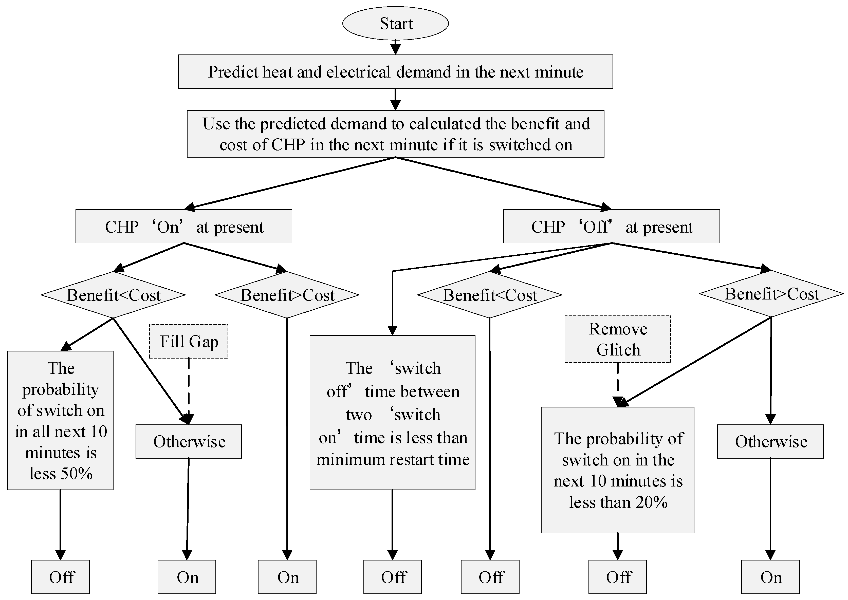
After getting the ‘probability of CHP switch on’ in each minute in a day, CHPS algorithm can be modified as:
- Step 1: Using Equations (6) and (7) to predict the next minute’s electricity demand and gas demand;
- Step 2: Comparing the benefit and cost of CHP in the next minute. If the benefit is greater than the cost, the state of CHP is set as ‘possible on’ and if the benefit is less than the cost, the state of CHP is set as ‘possible off’.
- Step 3: If the switch is ‘on’ at present and the state of CHP in next minute is predicted as ‘possible on’, the CHP is kept ‘on’ in the next minute. On the other hand, if the switch is ‘on’ at present and the state of CHP in the next minute is predicted as ‘possible off’, the state of CHP in the next minute will depend on the possible state of CHP in the next few minutes (10 min are used here). If in the next ten minutes, ‘the probability of CHP switch on’ is less than 50% for every individual minute—CHP will be shut down; otherwise CHP will be kept ‘on’.
- Step 4: If the switch is off at present and the state of CHP in the next minutes is predicted as ‘possible off’ the CHP will be kept ‘off’ in the next minute; however, if the state of CHP in the next minute is ‘possible on’; two situations should be taken into account. If the ‘probability of CHP switch on’ is less than 20% in all of the next ten individual minutes, this ‘possible on’ will be treated as a ‘Glitch’ and will be held in the off state. Otherwise CHP will be switched on in the following minute. To attempt to make full use of CHP, in this case, ‘probability of CHP switch on’ is set as 20%, rather than 50% as in step 3.
It is important to note that for all cases, the CHP cannot be switched on, if ‘switch off’ time between two ‘switch on’ times is shorter than CHP re-start time. Figure 3 is a flow diagram to show modified CHPS algorithm.
2.4. HESS Control Rule
Storage systems play an increasingly important role in modern energy systems. By regulating demand, they improve energy efficiency and thus reduce emissions. The energy cost can be greatly reduced, provided the HESS can be operated optimally. Moreover, storage technology has improved very quickly in recent years, specifically, smaller and lighter physical footprints and reduced cost [35], making them more practical in the domestic context. However, with the addition of a storage system, the energy systems’ complexity is greatly increased. With the inclusion of storage, the EH model requires a time domain treatment such that the full charge cycle of storage is considered, greatly increasing computational complexity. Additionally, it needs many converters, transformers and switches to connect HESS to the main energy system giving a more complex system topology.
2.4.1. Electrical Storage System (ESS) Control Rule
The purpose of the ESS is to support the CHP by reducing the reliance on grid imports during peak price periods and storing the surplus energy from the CHP switching, thus reducing the overall running cost of meeting the loads. However, this requires a precise control rule. Two things need to be considered carefully in advance—the amount of energy required to meet each electrical peak demand and the exact time to begin charging.
An ESS normally consists of a group of batteries, but in an Energy Hub system at building level, it is desirable to have more than one group of batteries due to the high frequency of charge cycles required. Compared with large electrical systems, the electricity demand at building level has higher uncertainty, thus the states (charging and discharging) of ESS may need to be changed very frequently. However, the life span of batteries will be significantly reduced if the states of batteries are changed too frequently. In [36], the authors describe that a simple two-battery system has a longer life span compared with a single battery system which has the same capacity.
In this paper, the ESS consists of two groups of batteries, and two batteries are used separately to supply the electrical load at the two daytime peak demands (shown in Figure 4).
In Figure 4, the first battery is charged before the morning peak, TP1, and discharged to compensate energy shortage for the first peak demand time TP2. (The energy shortage in the first peak demand time is the difference between electrical energy generated by CHP and the building’s electrical demand). The second battery is charged from very early in the morning to the beginning of the second peak TP1 to TP3 and then discharged to compensate energy shortage for the second peak, TP4. The electricity used to charge batteries is normally the surplus electricity generated by the CHP system. Very occasionally, electricity from the grid is used to charge the battery.
The two-battery storage system control algorithm is shown in the flowchart in Figure 5 and is as follows.
Step 1: Find each of the two daily peak demand start and end times and calculate how much energy should be stored in advance for each peak. This can be done by analysing the historical data from the same month of the previous year and using the curve fitting algorithm described in [33].
Step 2: After finding the first peak demand start time (), and the amount of energy shortage for the first peak demand (), the amount of theoretical surplus electrical energy ( in kilowatt hour) generated in each minute before the first peak can be calculated.
In Equation (11), is CHP rated power in Watts, is CHP electrical efficiency, t is time in minutes and is the average historical electricity consumption in the ith minute, in Joules. is the theoretical surplus electrical energy that can be stored in the ith minute.
Step 3: Then, the vector needs to be modified to get the total surplus electrical energy () in each minute generated by CHP before the beginning of the first peak. To be specific, change all the values in the vector whose value is less than zero to zero, and keep other terms the same, producing a modified vector . The formula of total energy can be stored before first peak start can be written as:
Step 4: Comparing and , find the highest value of that makes greater than . Record the value of and is the best time to charge the first battery ().
Step 5: Use the same method to calculate the total theoretical surplus electrical energy in each minute generated by the CHP between the start of the first peak and the start of the second peak. Compare with energy shortage for the second peak (), if is greater than , record the value of , and this is the theoretical best time to charge the second battery. However, if is less than calculate the difference between the two values and record it as , and then calculate the total theoretical surplus electrical energy in each minute generated by CHP before the best time to charge the first battery . Comparing and the , find the maximum value of and that is the theoretical best time to charge the second battery.
Step 6: Set the initial energy of the two groups of batteries. By carefully choosing the battery initial energy, ESS efficiency can be improved. Because the standby loss will be greater, if the initial energy in batteries is too high; on the other hand, if the initial energy is very low, the life span of battery will be reduced and less energy can be used as backup energy when the peak demand time extends or it comes earlier. This step is empirical and dependent on the particular system parameters, an example is shown in Section 4.3.
Step7: After the end of the second peak, both batteries need to be charged or discharged to the initial value. This usually involves charging both batteries since they have previously supplied the two load peaks. Therefore, even if the CHP cannot be used to recharge the batteries, this approach uses cheaper grid electricity during the cheaper night time period.
2.4.2. Heat Storage System (HSS) Control Rule
Compared with ESS, the Heat Storage System (HSS) has lower overall efficiency (i.e., charging efficiency and discharging efficiency), and a higher standby loss as quantified in Section 3. In addition, the gas price is likely to remain static on an hourly basis whereas domestic electricity price will soon become dynamic in most developed countries. Despite this, the static gas price is likely to remain always cheaper for some time. Therefore, under these conditions, the use of a boiler to heat water in advance is not justified. For HSS control, HSS is only charged by the redundant heat generated by CHP and discharged when it is required. Heat is then dispatched when it is needed, from the supplies with the following priority order 1. CHP (if it is ‘ON’), 2. HSS, 3. Gas via the boiler.
2.5. Theoretical Minimum Daily Operation Cost
To evaluate the performance of the proposed EH optimisation, this section will introduce a method to calculate the theoretical minimum daily operation cost for the EH shown in Section 2.1. This calculation assumes the system has perfect load predication, the CHP output can be varied from 0 to its maximum rated output, the efficiency at any output is its rated efficiency and there is no delay between the set point and actual output. Therefore, it gives the most conservative base case against which to evaluate the efficacy of the algorithm proposed in this paper.
This calculation consists of five steps. First, by comparing the electrical demand and maximum electrical output of CHP, find the first and last time that the electrical demand is greater than CHP electrical output in each high/intermediate price time. Calculate the amount of electrical energy shortage (EES) during each high price time and intermediate price time based on Equation (13):
In Equation (13), Esn is EES for the nth high/intermediate price time. is the sum of the electrical energy consumption calculated during the nth high/intermediate price time when electrical energy generated by CHP is less than demand and T is the total time that electrical energy generated by CHP is less than demand during nth high/intermediate price period. This assumes the CHP capacity is rated such that at certain peak times of electrical demand it will not be able to meet the demand.
Second, calculate redundant electrical energy that can be stored during nth high/intermediate price period if the CHP is working at rated power.
where Enstore is total electrical energy that can be stored for nth high/intermediate price time. is the sum of the electrical energy consumption calculated during the nth high/intermediate price time when electrical energy generated by CHP is greater than electrical demand and T’ is the total time that electrical energy generated by CHP is greater than demand during nth high/intermediate price period. is battery charging efficiency.
The third step is to find the differences between EES in step 1, and redundant energy that can be stored during the nth high/intermediate price period from step 2. Using the same method as proposed in Section 2.4, find the best time that CHP needs to work at the rated power to charge the battery. Using the maximum CHP output here avoids storage standby losses as much as possible because charging occurs at the latest possible period before the energy is required.
After finding the time that CHP should work at the rated power, the next step of this calculation is to control the output power of CHP at other times of day. At these times, if the electrical demand is greater than CHP electrical power generation, CHP must work at its rated power. If electrical demand is less than rated CHP electrical output, CHP output power should just meet electrical demand. This step considers the electricity tariff and battery overall efficiencies. Also at this step, redundant heat generated by CHP can be stored by the heat storage system and when the CHP output cannot meet the heat demand, the heat storage system will be prioritised to supply the heat load.
Finally, calculate the electricity and the gas bought from the grid. The gas price contains two components: gas used to supply the boiler and gas used to supply the CHP. The theoretical minimum operation cost of an Energy Hub can be written as:
In Equation (15), CTheo, Cgrid, Cchp and Cboiler are the theoretical minimum operation cost, electricity costs bought from grid, CHP operation cost and boiler operation cost. In the following section, a case study will be used to illustrate both the aforementioned methodology and compared against the minimum theoretical cost.
3. A Case Study
In this paper, a detached domestic building in the UK of approximately 30 years in age, occupied by four people is analysed. Daily electricity consumption in this paper was randomly generated by the CREST electricity model [37]. In order to simulate statistically realistic historical data, 50 groups of each month’s electricity consumption time series were generated with this model is used test the proposed algorithm. The electricity tariff is obtained in [38], which proposes a dynamic system of tariffs which vary on a half hourly timescale. Daily heat consumption in this building was generated by the model developed by Strathclyde University [34]. The daily gas price is based on current UK domestic gas price which is around 5 pence/kWh. Figure 6 and Figure 7 are used to show daily energy tariffs and average energy demands.
The Energy Hub model of this building is shown in Figure 2. In this building, the boiler burns gas to generate heat. Additionally, a high cost, high efficiency energy generator—a fuel cell CHP unit is used to generate heat and electricity together. Moreover, redundant electricity and heat can be stored in the batteries and water tank storage system to improve energy efficiency and reduce daily operation cost. The output power of CHP is 3 kW and its heat conversion efficiency is 66% and electricity conversion efficiency 22%. For heat boiler, gas to heat conversion efficiency is 88%. The overall efficiency of the battery system is 80% [39] and the standby loss for battery system is 3% per month [3]. The overall efficiency of heat storage system is 75% [40] and standby loss is 15% a day.
It is worth noting that this paper is designed to verify the efficacy of the proposed algorithm for a domestic user who has already installed the aforementioned infrastructures, with no need to consider the optimal capacity for each infrastructure, because the rated capacities of the aforementioned infrastructures used in this paper are based on the references of [41,42], in which many constraints, for example, battery SOC, are considered when sizing CHP and batteries. Additionally, the depreciation of energy infrastructures is not considered in this paper.
4. Optimisation Results
For a domestic building, the energy tariffs and demands which are shown in Figure 6 and Figure 7, yield a daily gas cost of 293 pence and a daily electricity cost of 308.45 pence. In this case, the daily operational cost for a domestic building is 601 pence without any optimisation Algorithm. The following section will be used to show daily operational cost with CHP control algorithm.
4.1. CHP Control Algorithm Optimisation
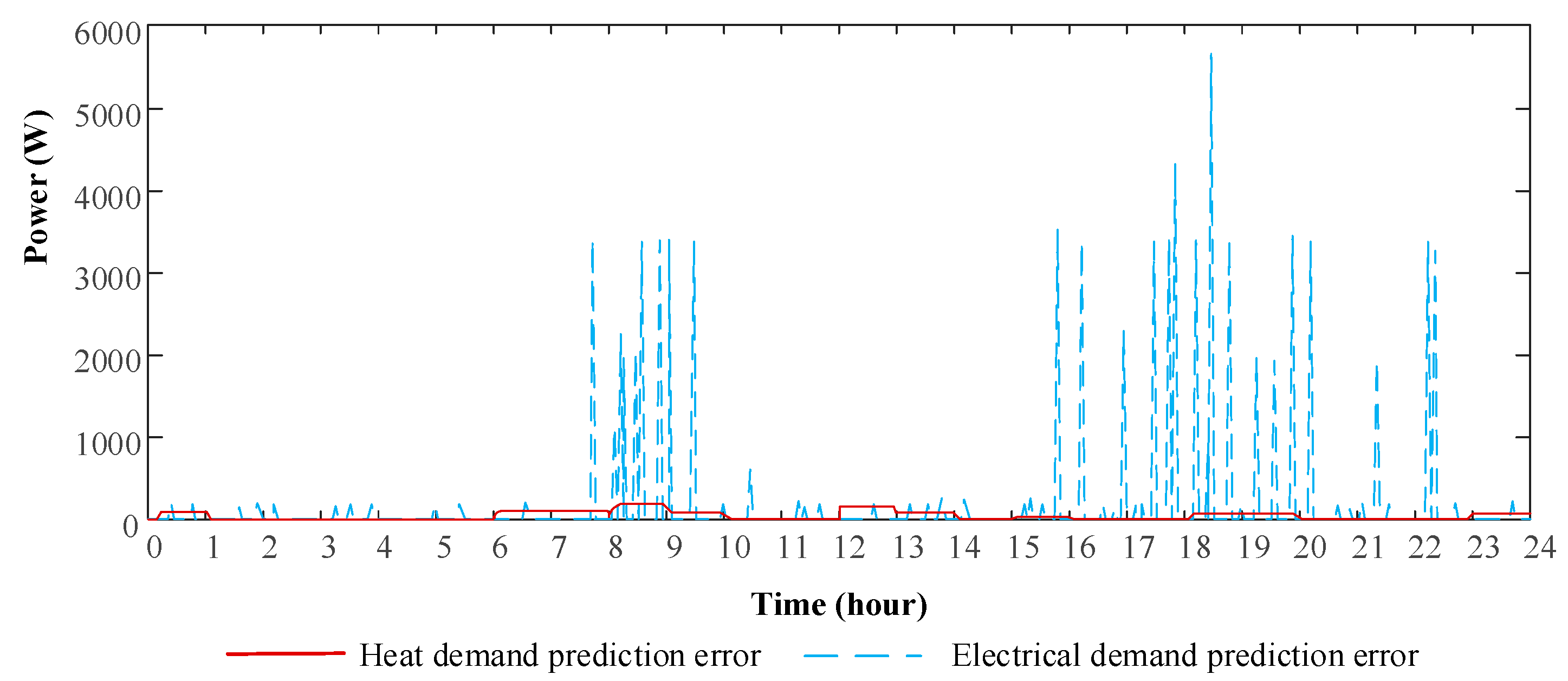
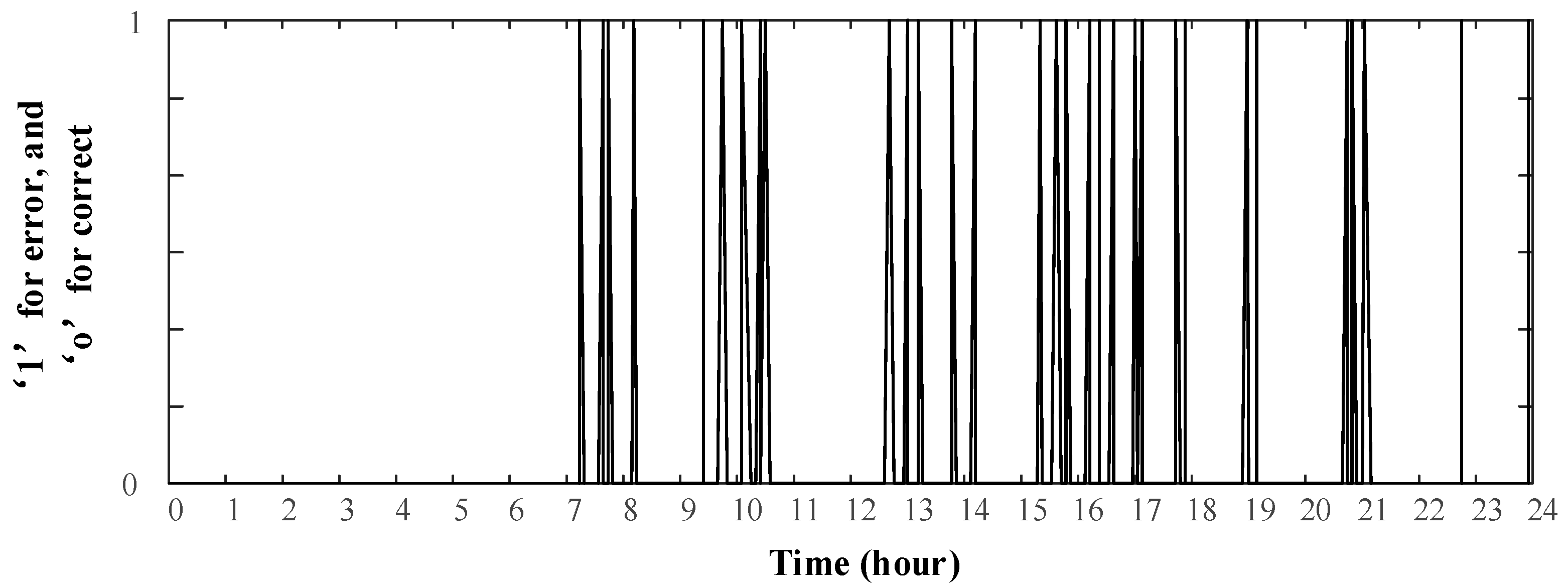
To get a more precise CHP control result, load prediction plays a crucial role. Based on simple load prediction rule proposed by Equations (6) and (7), Figure 8 shows the differences between the actual demands and the predicted demands. Figure 8 reveals that the electrical demand prediction error can be very high compared to the heat demand prediction error. However, when using the predicted demands just to control binary CHP, as discussed in Section 2.2 and shown in [33], this approach gives a low error rate, which is 2.9% in this particular case study. Figure 9 shows the times that the CHP control algorithm generates errors in typical day.
By applying the CHP control algorithm, the domestic building energy operational cost is reduced to 563 pence, which offers 38 pence saving a day. However, by applying this algorithm, the state of CHP changes very frequently, especially at night peak demand time. This is shown in Figure 11. In Figure 11, the dotted line shows the state of CHP in a day with the CHP control algorithm. To reduce dynamic ramp up times and cycling stress on the CHP, it is necessary to reduce the CHP switching frequency.
4.2. Modified CHP Control Algorithm
To reduce the CHP switching frequency, ‘Remove Glitch’ and ‘Fill Gap’ methods are used in this paper, as described in Section 2.3. In order to distinguish a CHP state signal as ‘Glitch’ or ‘Gap’, the probability of CHP ‘switch on’ in each minute needs to be acquired in advance. Figure 10 shows the probability of CHP ‘switch on’ of all the days in averaged. After getting the probability of CHP switch on, the modified CHP switch state can be acquired and it is shown in Figure 11. In Figure 11, the solid line shows modified CHP state in that day.
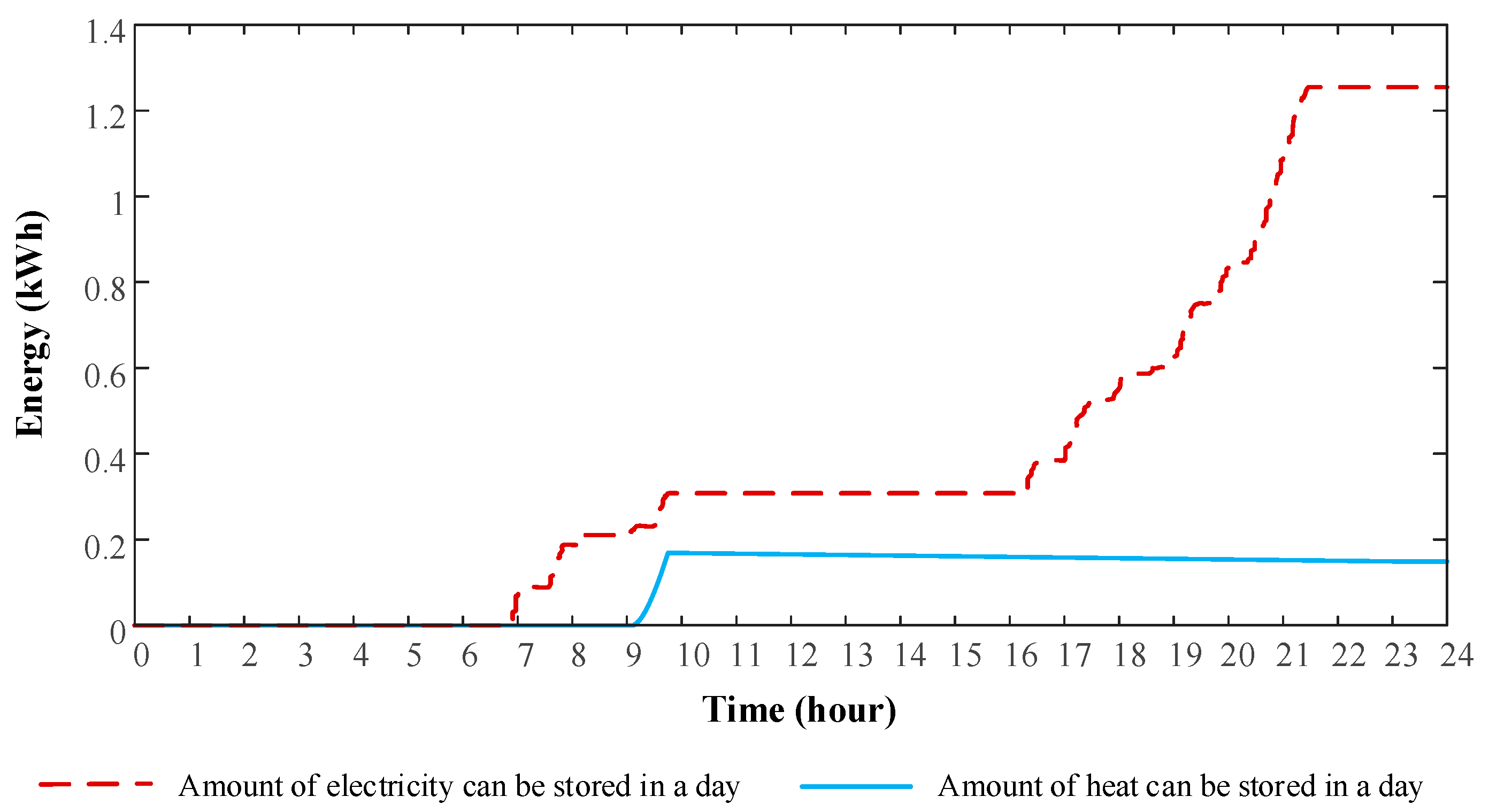
Compared to the standard CHP control algorithm, the modified CHP switch algorithm has successfully reduced switching frequency through ‘Fill Gap’ and ‘Remove Glitch’. However, ‘Fill Gap’ and ‘Remove Glitch’ increases system operational cost slightly to 566 pence, which is about 3 pence higher than the CHP control model. Simply using CHP control model can reduce the energy cost for the domestic building; however, energy efficiency is reduced due to the redundant energy generated by CHP. Figure 12 shows the total electrical energy and heat energy that can be stored if the energy storage system is available. After calculation, total redundant heat generated by the CHP is 0.197 kWh and the redundant electricity is 1.33 kWh.
4.3. Energy Storage System Control Algorithm
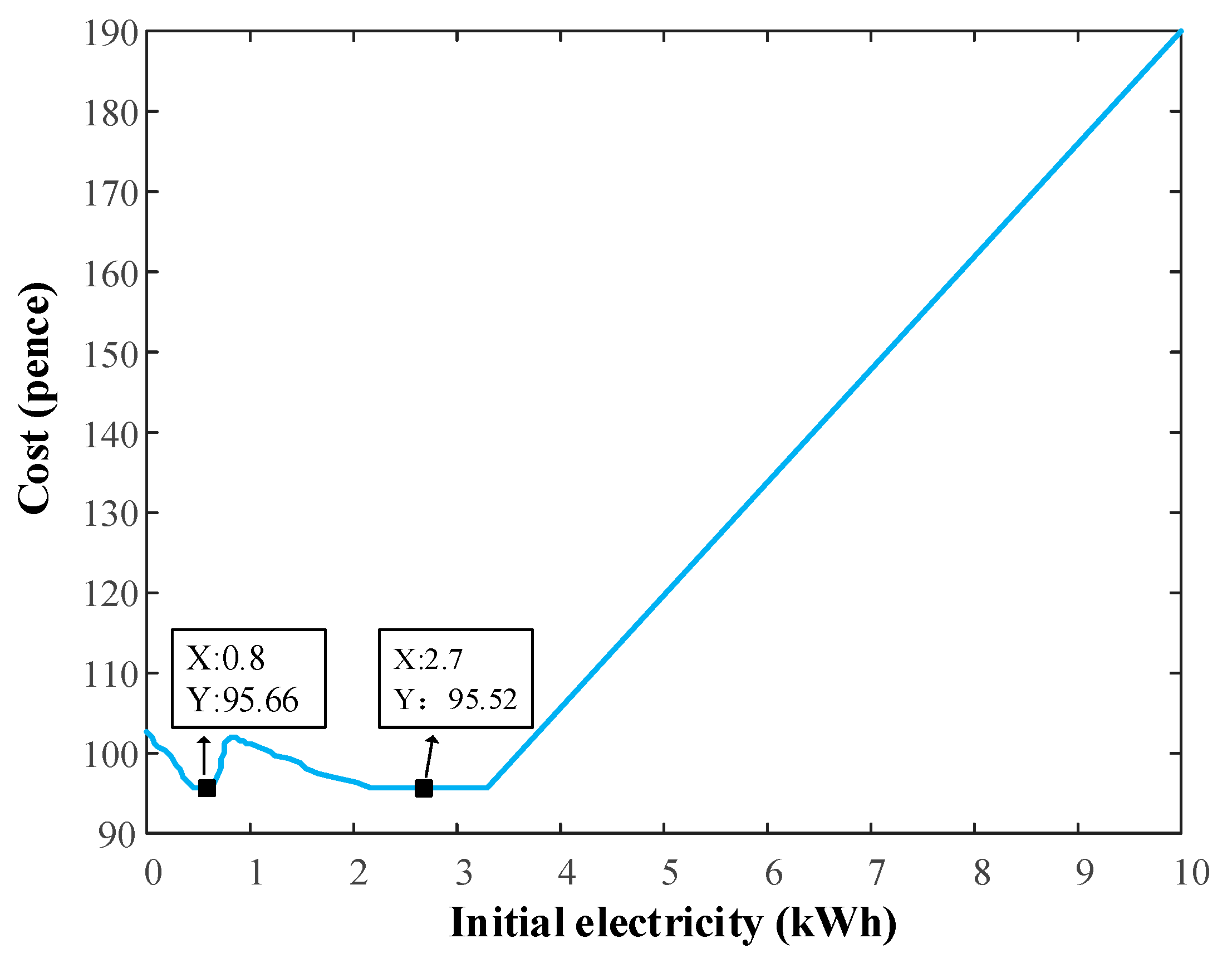
Aforementioned in Section 2.4, by carefully choosing the initial value of energy storage system, the operational cost for energy storage system can be reduced to some extent. Considering the high standby loss of the heat storage system and the flat rate of gas price, it is preferable not to store heat in advance. Thus, the initial heat in HSS is set to 0 kWh. However, considering the electricity tariff can change significantly in a day and the standby loss for electrical storage system is relatively small, storing a reasonable amount of electrical energy in advance can improve overall system cost. Figure 13 shows electricity cost of the domestic building against initial energy stored in the electrical storage system. This was produced using a fixed base case combining the overall management system shown in Figure 1 and the initial parameters in Section 3.
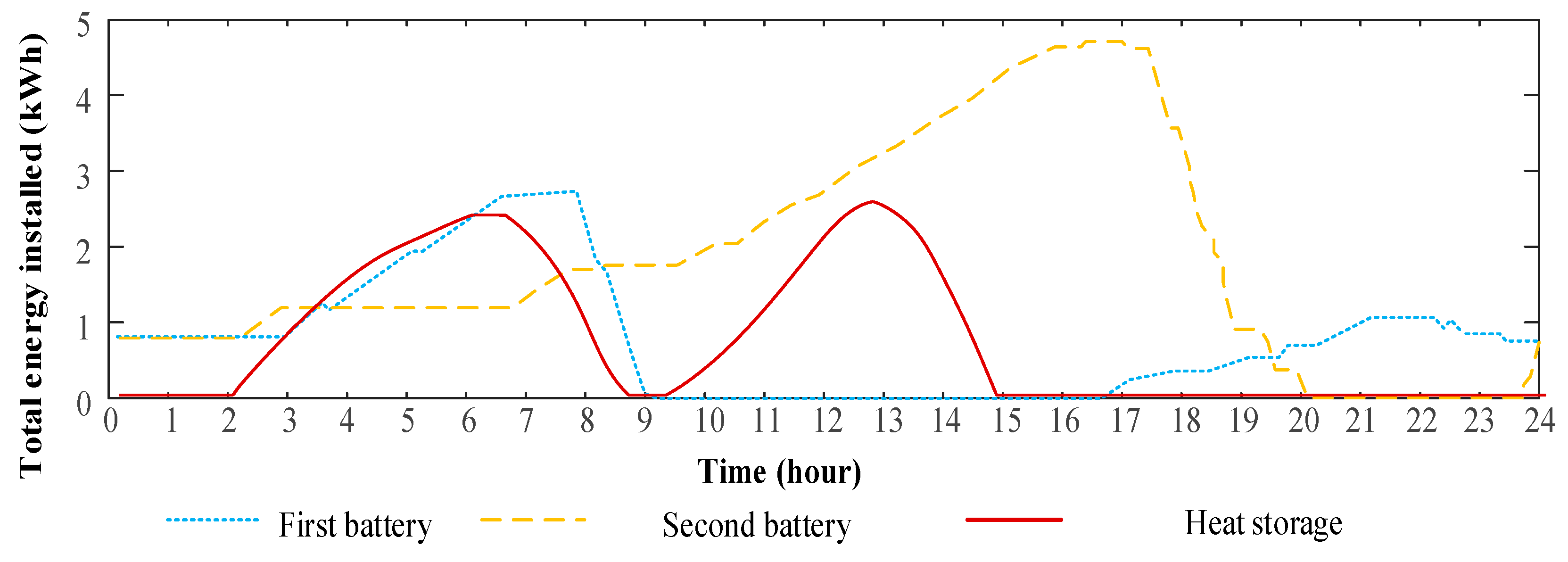
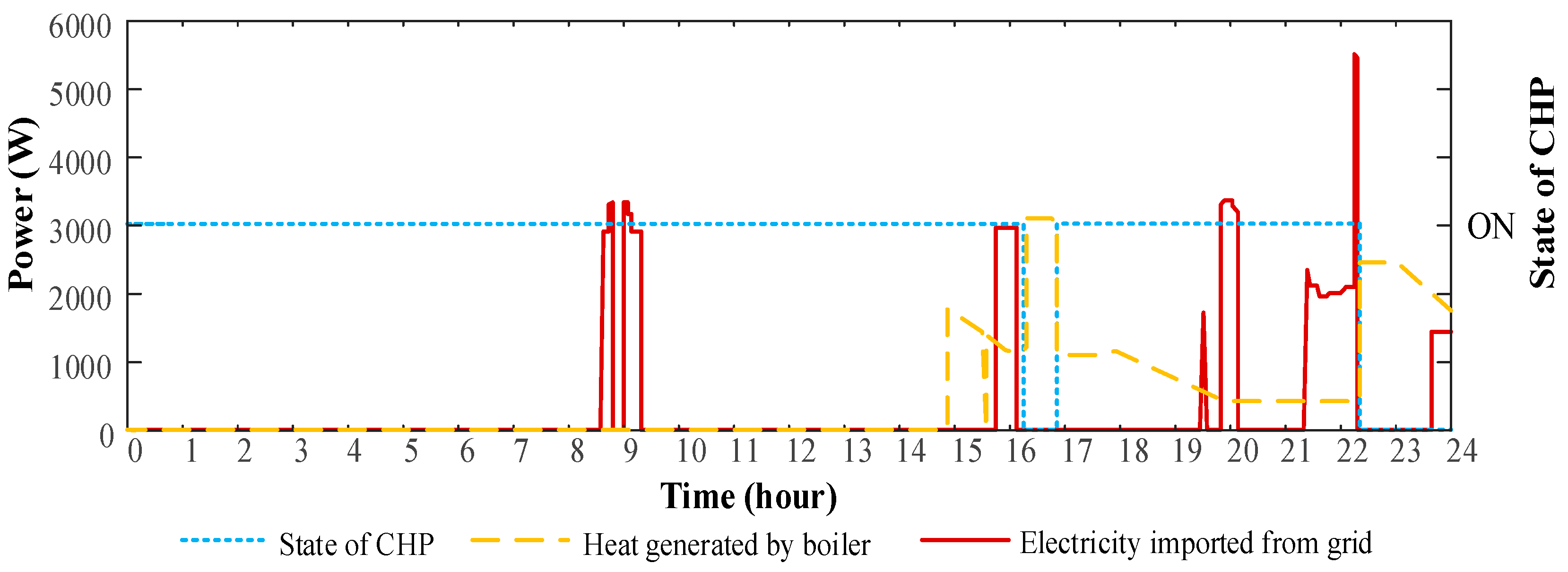
From Figure 13, the daily electricity cost will be the lowest if initial electrical energy is set as 0.8 kWh. After setting the initial energy for the energy storage system and operating it as demonstrated in Section 2.4, the amount of imported gas, electricity and the state of CHP can be acquired. Figure 14 shows the state of CHP, the amount of imported gas and electricity in a day based on proposed Energy Hub optimisation rules in this paper. Figure 15 shows the amount of energy which is stored in battery one, battery two and the hot water tank respectively.
With the installation of the energy storage system, daily energy cost can yield a further reduction. Based on the control algorithm, total operational cost now reduces to 464 pence, which saves about £1.38 a day. Specifically, the cost of electricity imported from grid is 91 pence, the gas that used to supply heat demand is 74 pence and the remaining cost of 299 pence is used to import gas to supply the CHP. With the proposed optimisation rules, the total cost reduction is 22.9%, which is a 2.9% improvement on previous similar work which reduces cost by 20% [10]. Therefore, the algorithm represents a 14.5% improvement on previous work.
4.4. Theorectical Minimum
As shown in Table 1, using the calculation shown in Section 2.5, the theoretical minimum operation cost for sampling day is 449 pence. To get the theoretical minimum, the cost of electricity imported from the grid is 58 pence, the gas that is used to supply the heat demand is 31 pence and the remaining cost of 360 pence is used to import gas to supply the CHP.
By comparing two results, it is easy to find that the cost from the combined hub control algorithm is very close to the theoretical minimum, and the ratio of cost from the theoretical minimum to the combined hub control algorithm cost is over 96.8%. This ratio varied from 88.8% to 97% after testing the whole year’s data and clearly strongly depends on the daily load profile. If the daily average electrical load is very high, the CHP may need to operate at the rated power for the whole day, and this will reduce the difference between the proposed algorithm’s cost and theoretical minimum. Thus, in this case the ratio is very high and the proposed method is very effective. However, it is worth noting that the theoretical minimum is calculated using conservative assumptions such as perfect CHP efficiency and instantaneous output. Therefore, the whole range of ratios will be somewhat improved when real world imperfections are accounted for. It can thus be stated with some confidence that the algorithm presented here always yields better than 88% of the theoretical minimum cost.
5. Conclusions
The proposed rule based Energy Hub optimisation algorithm reduces the complexity of computation, improves system dynamic performance (the time step in this paper is one minute compared to previous work which an hour or half hour) and further reduces system operational cost by 2.92% a day compared with previous work, representing a 14.5% improvement on previous work. The optimisation approach is more real world feasible, because in this paper, it is assumed that CHP has binary states of operation. This assumption reduces the time delay between set points and actual output arising from dynamic operation of CHP, therefore reducing inaccuracy in the optimisation when deployed in the real world. Meanwhile, it maximises the CHP efficiency by reducing energy loss since when in operation the plant operates for longer at full capacity. Finally, the modified CHP control algorithm reduces the cycling stress on the CHP extending the plant lifetime. For the first time in the context of domestic CHP, dual battery storage systems are deployed together to store surplus electricity thus extending the life time of each battery.
The daily energy cost from the combined hub control algorithm is 464 pence, which gives about £1.38 energy saving a day. In the case study, the ratio between the control algorithm’s savings and the theoretical minimum savings are over 96.8%, and are shown to be always over 88% for a whole year’s data, using conservative theoretical minimum assumptions, showing that this is a very powerful algorithm to optimise energy consumption in a domestic building.
To further increase daily saving, there are four suggested approaches. The first one is to increase cost from the combined hub control algorithm to theoretical minimum ratio. To increase this rate, more precise ‘Gap’ and ‘Glitch’ diagnostic system needs to be built. However, this will significantly extend computation time and system complexity. The second way is to reduce theoretical minimum cost itself which can be achieved by improving storage system efficiencies and improving CHP generation efficiencies. This will happen as individual technologies improve. Thirdly, careful sizing of the CHP capacity is important because too small a plant will lead to an energy shortage that must be supplied by the grid, whereas too large will not justify the benefit of CHP turn-on to meet load. By optimising the CHP capacity both the efficacy of the combined hub control algorithm in reaching the theoretical minimum can be increased, and at the same time, the theoretical minimum itself can be reduced. This is the most promising way to reduce optimal operational cost. Finally, as suggested by [43], domestic users may benefit from building interconnection with many local energy systems through importing energy from different local energy systems based on the price factor.
Acknowledgments
Supported by special fund project of Beijing key laboratory (Z171100002217071) and innovation fund project of China Electric Power Research Institute (YD83-17-002).
Author Contributions
Dongmin Yu and Xinyi Xu conceived and designed the experiments; Huanan Liu analyzed the data; Mingyu Dong revised the paper; Dezhi Li wrote the paper.
Conflicts of Interest
The authors declare not conflict of interest.
References
- Bozchalui, M.C.; Canizares, C.A.; Bhattacharya, K. Optimal Energy Management of Greenhouses in Smart Grids. IEEE Trans. Smart Grid 2015, 6, 827–835. [Google Scholar] [CrossRef]
- Erdinc, O.; Paterakis, N.G.; Mendes, T.D.; Bakirtzis, A.G.; Catalão, J.P. Smart Household Operation Considering Bi-Directional EV and ESS Utilization by Real-Time Pricing-Based DR. IEEE Trans. Smart Grid 2015, 6, 1281–1291. [Google Scholar] [CrossRef]
- Mishra, A.; Irwin, D.; Shenoy, P.; Kurose, J.; Zhu, T. Greencharge: Managing Renewable Energy in Smart Buildings. IEEE J. Sel. Areas Commun. 2013, 31, 1281–1293. [Google Scholar] [CrossRef]
- Houwing, M.; Negenborn, R.R.; de Schutter, B. Demand Response with Micro-CHP Systems. Proc. IEEE 2011, 99, 200–213. [Google Scholar] [CrossRef]
- Abdmouleh, Z.; Gastli, A.; Ben-Brahim, L. Review of optimization techniques applied for the integration of distributed generation from renewable energy sources. Renew. Energy 2017, 113, 266–280. [Google Scholar] [CrossRef]
- Atwa, Y.M.; El-Saadany, E.F.; Salama, M.M.A.; Seethapathy, R. Optimal Renewable Resources Mix for Distribution System Energy Loss Minimization. IEEE Trans. Power Syst. 2010, 25, 360–370. [Google Scholar] [CrossRef]
- Parra, D.; Walker, G.S.; Gillotta, M. Are batteries the optimum PV-coupled energy storage for dwellings? Techno-economic comparison with hot water tanks in the UK. Energy Build. 2016, 116, 614–621. [Google Scholar] [CrossRef]
- Olabi, A.G. Renewable energy and energy storage systems. Energy 2017, 136, 1–6. [Google Scholar] [CrossRef]
- Zhang, X.; Chen, H.; Xua, Y.; Li, W.; He, F.; Guo, H.; Huang, Y. Distributed generation with energy storage systems: A case study. Appl. Energy 2017, 204, 1251–1263. [Google Scholar] [CrossRef]
- Bozchalui, M.C.; Hashmi, S.A.; Hassen, H.; Cañizares, C.A.; Bhattacharya, K. Optimal Operation of Residential Energy Hubs in Smart Grids. IEEE Trans. Smart Grid 2012, 3, 1755–1766. [Google Scholar] [CrossRef]
- Yin, Z.; Che, Y.; Li, D.; Liu, H.; Yu, D. Optimal Scheduling Strategy for Domestic Electric Water Heaters Based on the Temperature State Priority List. Energies 2017, 10, 1425. [Google Scholar] [CrossRef]
- Geidl, M.; Koeppel, G.; Favre-Perrod, P.; Klockl, B.; Andersson, G.; Frohlich, K. Energy Hubs for the future. IEEE Power Energy Mag. 2007, 5, 24–30. [Google Scholar] [CrossRef]
- Neyestani, N.; Yazdani-Damavandi, M.; Shafie-Khah, M.; Chicco, G.; Catalão, J.P. Stochastic modeling of multienergy carriers dependencies in smart local networks with distributed energy resources. IEEE Trans. Smart Grid 2015, 6, 1748–1762. [Google Scholar] [CrossRef]
- Mongibello, L.; Capezzuto, M.; Graditi, G. Technical and cost analyses of two different heat storage systems for residential micro-CHP plants. Appl. Therm. Eng. 2014, 71, 636–642. [Google Scholar] [CrossRef]
- Peng, Z.; Suryanarayanan, S.; Simoes, M.G. An Energy Management System for Building Structures Using a Multi-Agent Decision-Making Control Methodology. IEEE Trans. Ind. Appl. 2013, 49, 322–330. [Google Scholar]
- Kienzle, F.; Ahcin, P.; Andersson, G. Valuing Investments in Multi-Energy Conversion, Storage, and Demand-Side Management Systems Under Uncertainty. IEEE Trans. Sustain. Energy 2011, 2, 194–202. [Google Scholar] [CrossRef]
- Pourmousavi, S.A.; Nehrir, M.H.; Sharma, R.K. Multi-Timescale Power Management for Islanded Microgrids Including Storage and Demand Response. IEEE Trans. Smart Grid 2015, 6, 1185–1195. [Google Scholar] [CrossRef]
- Moradi, M.H.; Eskandari, M.; Hosseinian, S.M. Operational Strategy Optimization in an Optimal Sized Smart Microgrid. IEEE Trans. Smart Grid 2015, 6, 1087–1095. [Google Scholar] [CrossRef]
- Sheikhi, A.; Rayati, M.; Bahrami, S.; Ranjbar, A.M. Integrated Demand Side Management Game in Smart Energy Hubs. IEEE Trans. Smart Grid 2015, 6, 675–683. [Google Scholar] [CrossRef]
- Brahman, F.; Honarmand, M.; Jadid, S. Optimal electrical and thermal energy management of a residential Energy Hub, integrating demand response and energy storage system. Energy Build. 2015, 90, 65–75. [Google Scholar] [CrossRef]
- Rastegar, M.; Fotuhi-Firuzabad, M.; Lehtonen, M. Home load management in a residential Energy Hub. Electr. Power Syst. Res. 2015, 119, 322–328. [Google Scholar] [CrossRef]
- Pehnt, M.; Cames, M.; Fischer, C.; Praetorius, B.; Schneider, L.; Schumacher, K.; Voß, J.-P. Micro Cogeneration: Towards Decentralized Energy Systems; Springer Science & Business Media: Berlin, Germany, 2006. [Google Scholar]
- Wang, Y.; Bermukhambetova, A.; Wang, J.; Lv, J.; Gao, Q. Dynamic modelling and simulation study of a university campus CHP power plant. In Proceedings of the 20th International Conference on Automation and Computing (ICAC), Cranfield, UK, 12–13 September 2014. [Google Scholar]
- Hernandez, L.; Baladron, C.; Aguiar, J.M.; Carro, B.; Sanchez-Esguevillas, A.J.; Lloret, J.; Massana, J. A Survey on Electric Power Demand Forecasting: Future Trends in Smart Grids, Microgrids and Smart Buildings. IEEE Commun. Surv. Tutor. 2014, 16, 1460–1495. [Google Scholar] [CrossRef]
- Amjady, N. Short-Term Bus Load Forecasting of Power Systems by a New Hybrid Method. IEEE Trans. Power Syst. 2007, 22, 333–341. [Google Scholar] [CrossRef]
- Amjady, N.; Keynia, F.; Zareipour, H. Short-Term Load Forecast of Microgrids by a New Bilevel Prediction Strategy. IEEE Trans. Smart Grid 2010, 1, 286–294. [Google Scholar] [CrossRef]
- Sargunaraj, S.; Gupta, D.P.S.; Devi, S. Short-term load forecasting for demand side management. IEE Proc. Gener. Transm. Distrib. 1997, 144, 68–74. [Google Scholar] [CrossRef]
- Di Somma, M.; Graditi, G.; Heydarian-Forushani, E.; Shafie-Khah, M.; Siano, P. Stochastic optimal scheduling of distributed energy resources with renewables considering economic and environmental aspects. Renew. Energy 2018, 116, 272–287. [Google Scholar] [CrossRef]
- Sheikhi, A.; Ranjbar, A.M.; Safe, F. A novel method to determine the best size of CHP for an Energy Hub system. In Proceedings of the 2nd International Conference on Electric Power and Energy Conversion Systems (EPECS), Sharjah, UAE, 15–17 November 2011. [Google Scholar]
- Geild, M. Integrated Modeling and Optimization of Multi-Carrier Energy Systems. Ph.D. Thesis, ETH Zurich, Zürich, Switzerland, 2007. [Google Scholar]
- Fabrizo, E. Modelling of Multi-Energy Systems in Buildings. Ph.D. Thesis, Politecnico di Torino, Torino, Italy, 2008. [Google Scholar]
- Le Blond, S.; Li, R.; Li, F.; Wang, Z. Cost and emission savings from the deployment of variable electricity tariffs and advanced domestic Energy Hub storage management. In Proceedings of the 2014 IEEE PES General Meeting|Conference & Exposition, National Harbor, MD, USA, 27–31 July 2014. [Google Scholar]
- Yu, D.; Robinson, F.; Zha, W.; Le Blond, S. Using Historical Data Processing Method to Optimize Energy Hub. In Proceedings of the International Universities Power Engineering Conference (UPEC), Stroke-on-Trent, UK, 1–4 September 2015. [Google Scholar]
- Yao, R.; Steemers, K. A method of formulating energy load profile for domestic buildings in the UK. Energy Build. 2005, 37, 663–671. [Google Scholar] [CrossRef]
- Boicea, V.A. Energy Storage Technologies: The Past and the Present. Proc. IEEE 2014, 102, 1777–1794. [Google Scholar] [CrossRef]
- Benini, L.; Bruni, D.; Mach, A.; Macii, E.; Poncino, M. Discharge current steering for battery lifetime optimization. IEEE Trans. Comput. 2003, 52, 985–995. [Google Scholar] [CrossRef]
- Richardson, I.; Thomson, M.; Infield, D.; Clifford, C. Domestic electricity use: A high-resolution energy demand model. Energy Build. 2010, 42, 1878–1887. [Google Scholar] [CrossRef] [Green Version]
- Wang, Z.; Gu, C.; Li, F.; Bale, P.; Sun, H. Active Demand Response Using Shared Energy Storage for Household Energy Management. IEEE Trans. Smart Grid 2013, 4, 1888–1897. [Google Scholar] [CrossRef]
- Kollimalla, S.K.; Mishra, M.K.; Narasamma, N.L. Design and Analysis of Novel Control Strategy for Battery and Supercapacitor Storage System. IEEE Trans. Sustain. Energy 2014, 5, 1137–1144. [Google Scholar] [CrossRef]
- Fan, J.; Furbo, S.; Yue, H. Development of a Hot Water Tank Simulation Program with Improved Prediction of Thermal Stratification in the Tank. Energy Procedia 2015, 70, 193–202. [Google Scholar] [CrossRef] [Green Version]
- Yu, D.; Meng, Y.; Yan, G.; Mu, G.; Li, D.; Blond, S.L. Sizing Combined Heat and Power Units and Domestic Building Energy Cost Optimisation. Energies 2017, 10, 771. [Google Scholar] [CrossRef]
- Yu, D.; Liu, H.; Yan, G.; Jiang, J.; Blond, S.L. Optimization of Hybrid Energy Storage Systems at the Building Level with Combined Heat and Power Generation. Energies 2017, 10, 606. [Google Scholar] [CrossRef]
- Damavandi, M.Y.; Neyestani, N.; Chicco, G.; Shafie-khah, M.; Catalao, J.P. Aggregation of Distributed Energy Resources under the Concept of Multi-Energy Players in Local Energy System. IEEE Trans. Sustain. Energy 2017, 8, 1679–1693. [Google Scholar] [CrossRef]
Figure 1.
Energy Hub optimisation algorithm proposed in this paper.

Figure 2.
An example of Energy Hub model that contains a combined heat and power (CHP), a boiler, a hybrid electrical storage system and a water tank heat storage system.
Figure 2.
An example of Energy Hub model that contains a combined heat and power (CHP), a boiler, a hybrid electrical storage system and a water tank heat storage system.
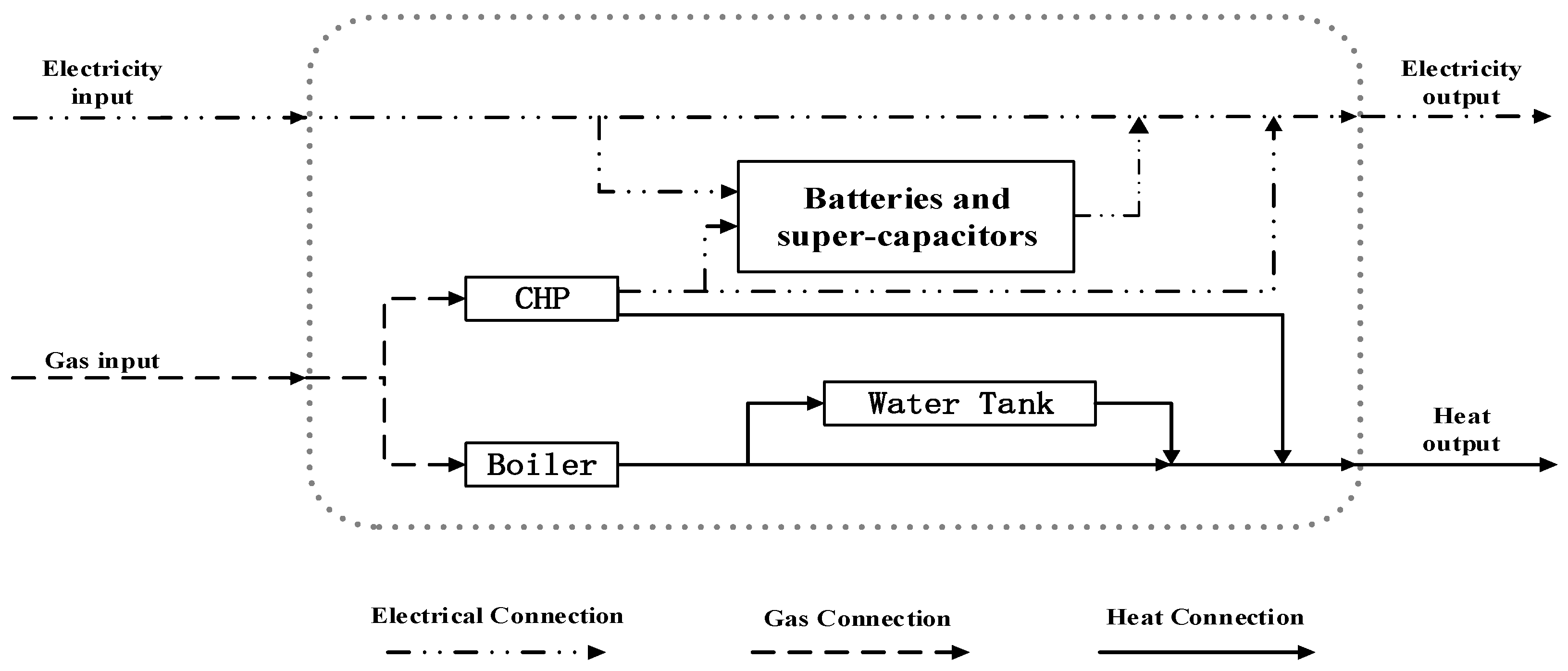
Figure 3.
Modified Combined Heat and Power Switch (CHPS) model.

Figure 4.
Two-battery storage system control rule.
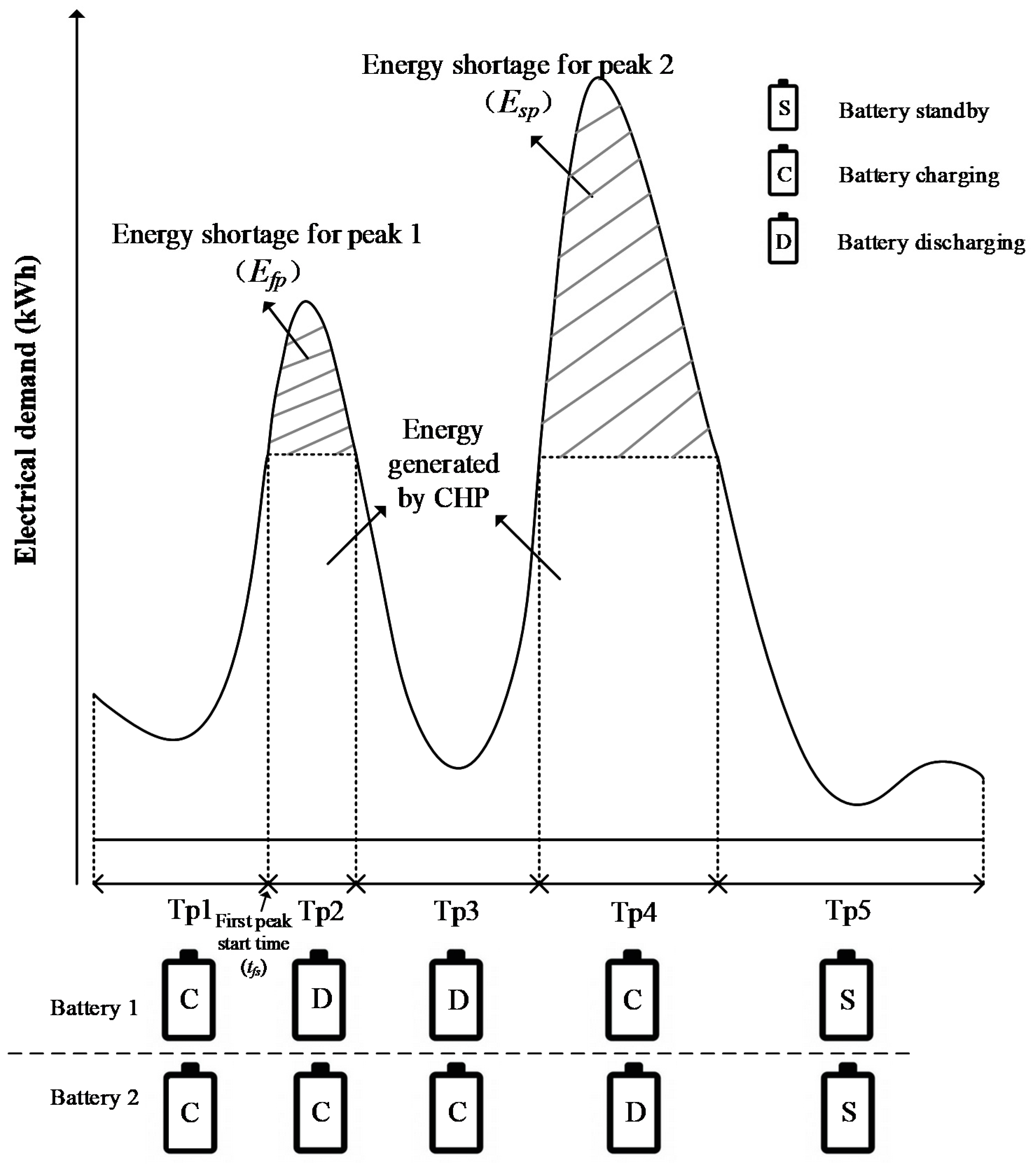
Figure 5.
Electrical Energy control rule.
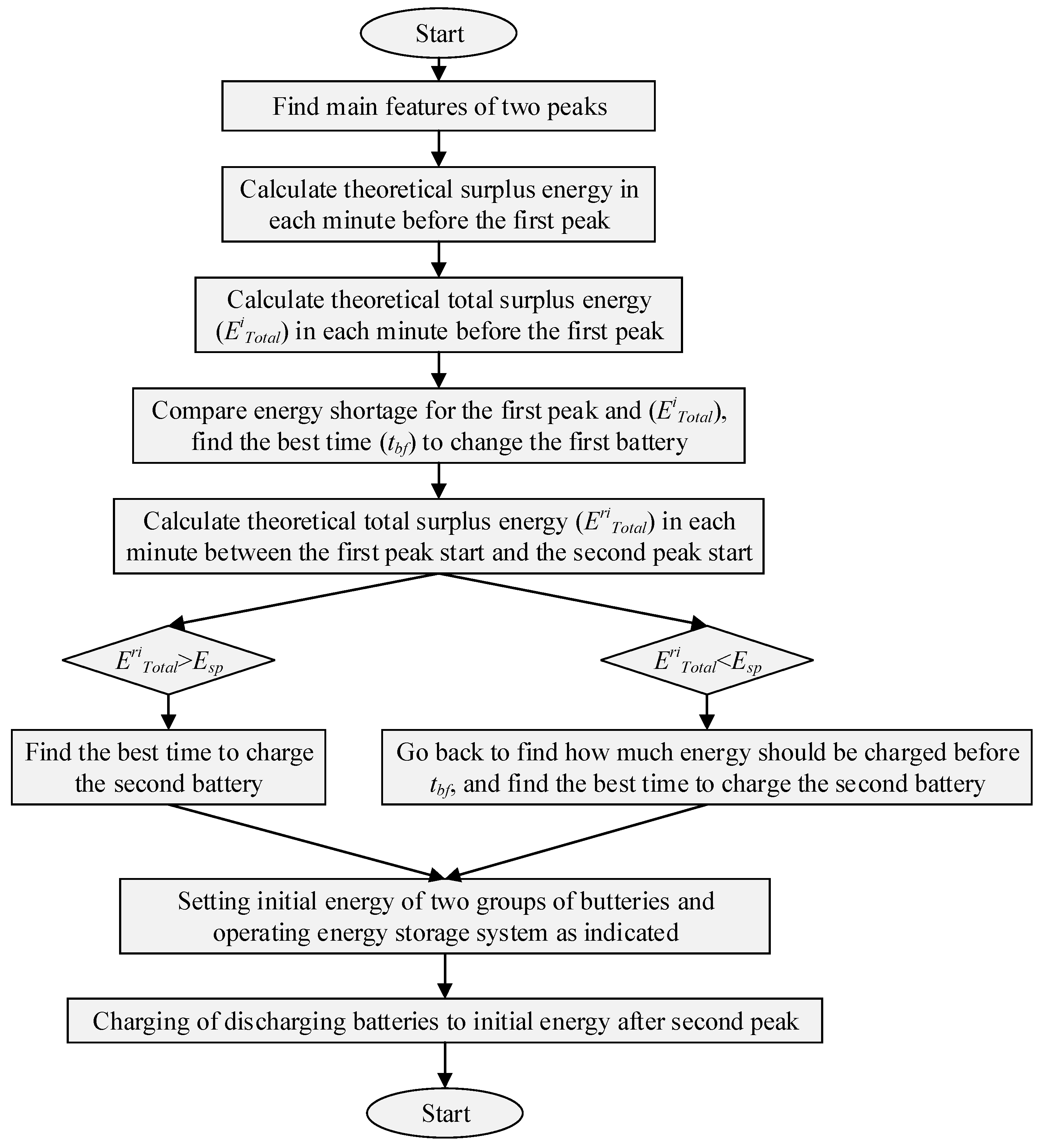
Figure 6.
Electricity and gas tariffs.
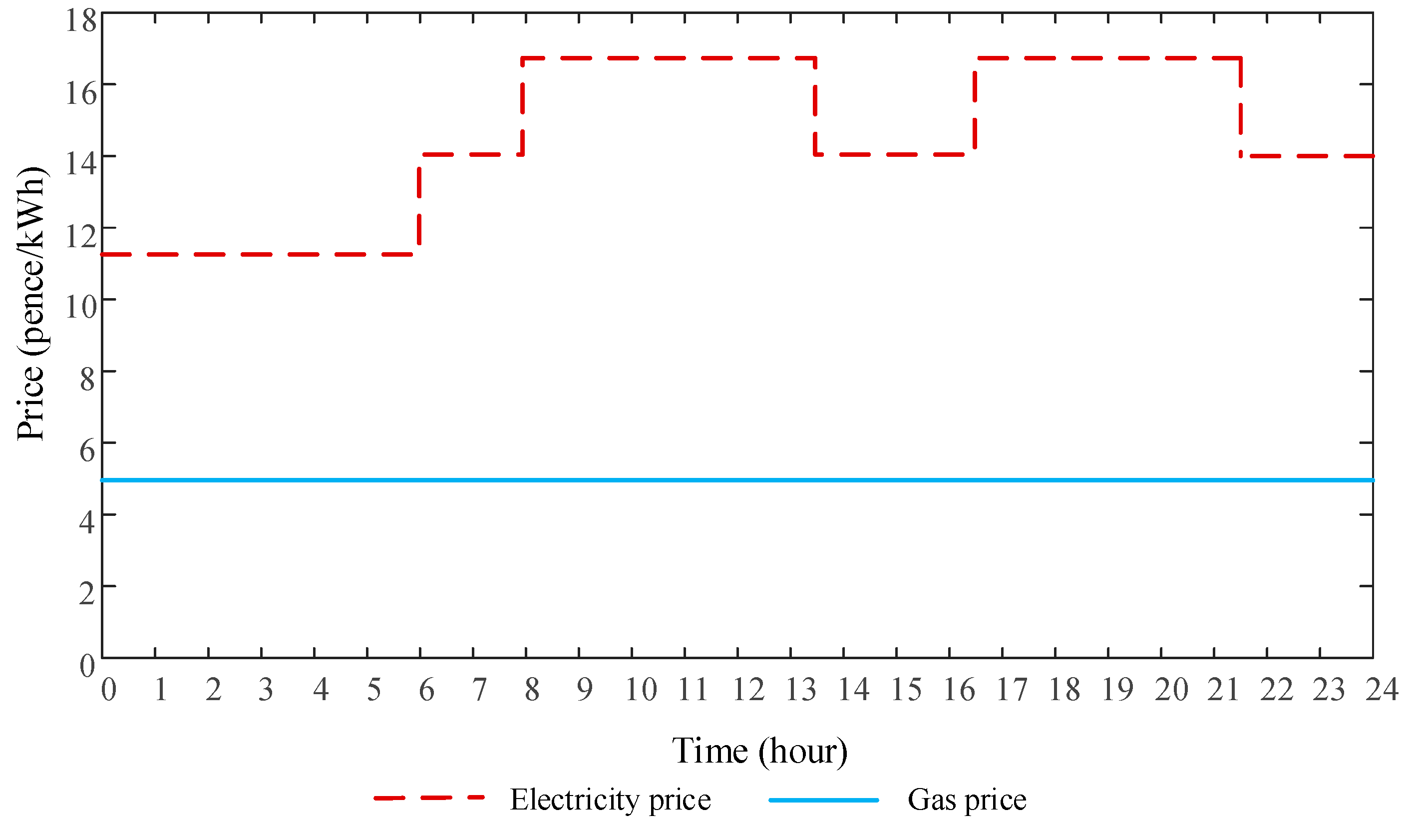
Figure 7.
An example of daily heat demand and Electrical Demand.
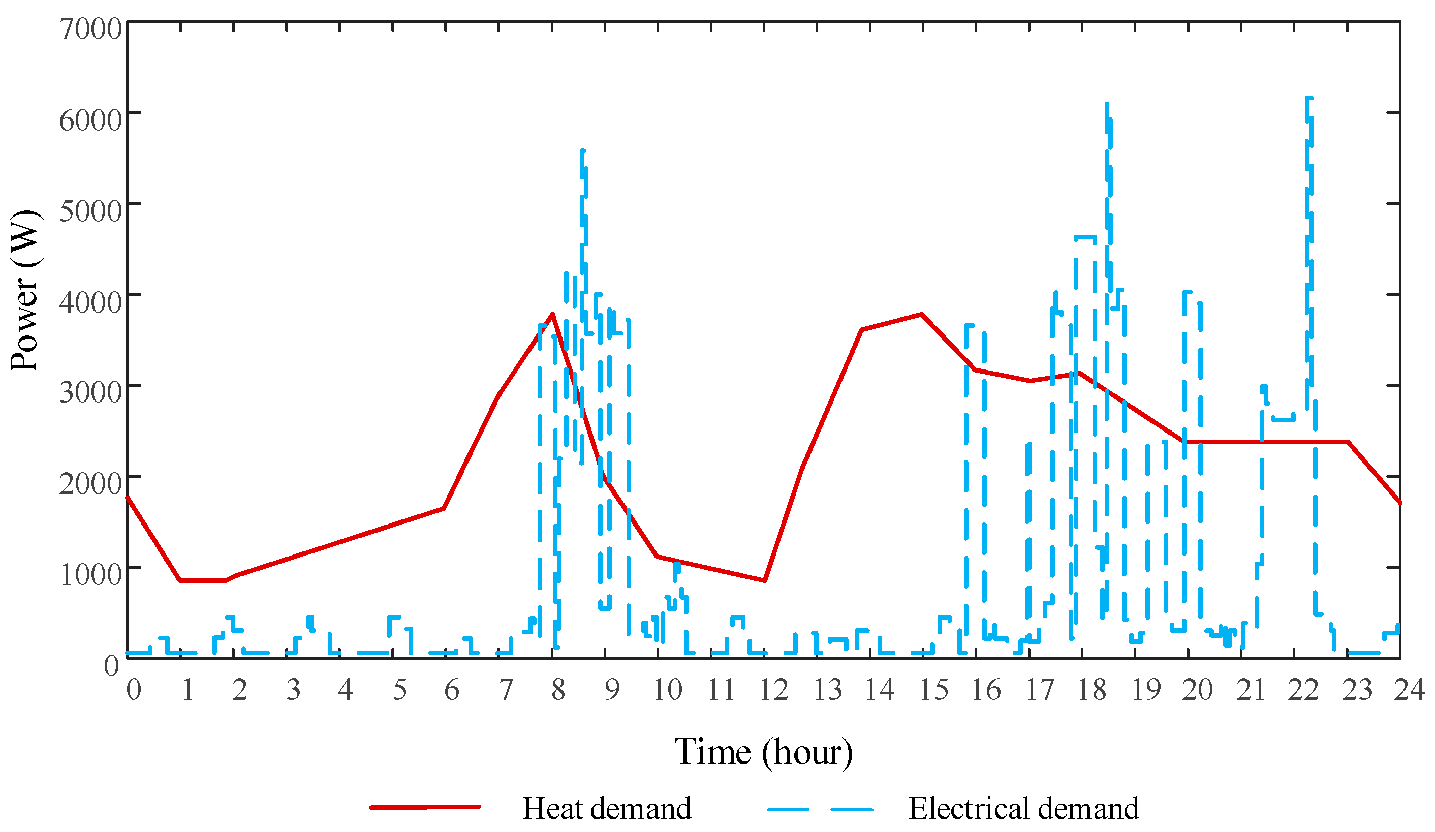
Figure 8.
Heat and electrical demand prediction error by using proposed prediction algorithm.

Figure 9.
The CHP control algorithm errors in sampling date.

Figure 10.
The probability of CHP Switch ‘ON’.
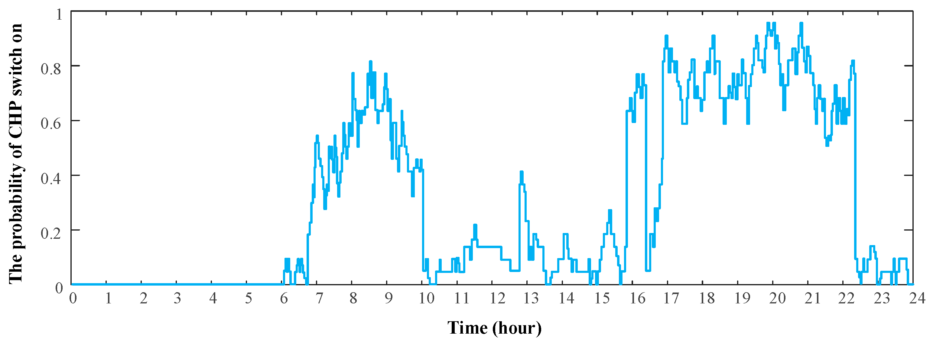
Figure 11.
The states of CHP by applying CHP control algorithm and modified CHP control algorithm.
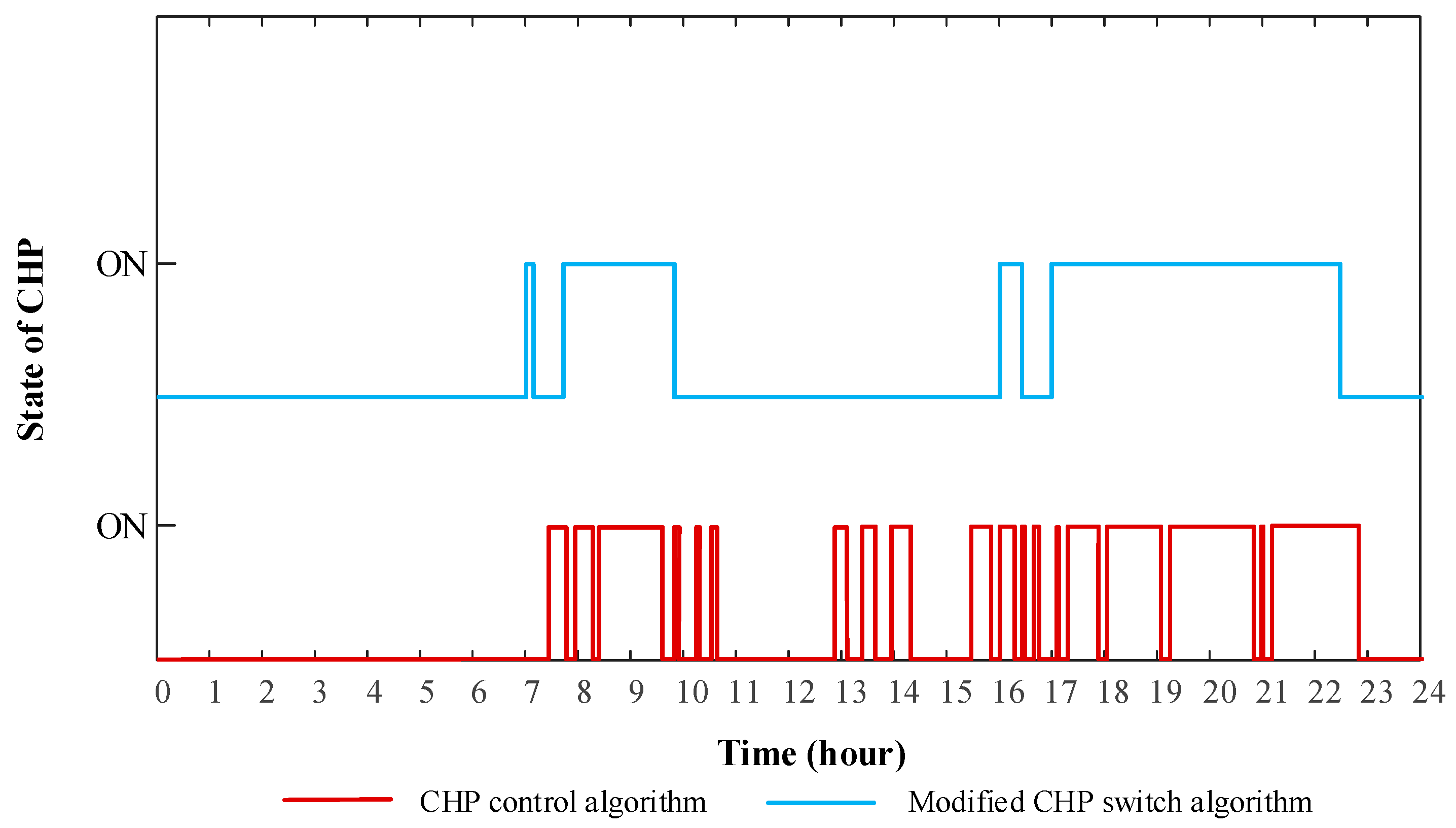
Figure 12.
The accumulative redundant energy can be stored in energy storage system by applying the modified CHP control algorithm.
Figure 12.
The accumulative redundant energy can be stored in energy storage system by applying the modified CHP control algorithm.

Figure 13.
Battery initial energy in (kWh) vs domestic building daily electricity cost.

Figure 14.
The state of CHP and the amount of imported gas and electricity in a day.

Figure 15.
Energy Stored in hot water tank and batteries.

Table 1.
Energy cost for in case study without algorithm, proposed algorithm and theoretical minimum.
Table 1.
Energy cost for in case study without algorithm, proposed algorithm and theoretical minimum.
| Algorithm | Gas Price (Used for CHP) (Pence) | Gas Price (Used for Heat) (Pence) | Electricity Price (Pence) | Total Price (Pence) |
|---|---|---|---|---|
| No algorithm | 293 | 293 | 309 | 602 |
| Proposed algorithm | 299 | 74 | 91 | 464 |
| Theoretical minimum | 360 | 31 | 58 | 449 |
© 2017 by the authors. Licensee MDPI, Basel, Switzerland. This article is an open access article distributed under the terms and conditions of the Creative Commons Attribution (CC BY) license (http://creativecommons.org/licenses/by/4.0/).
Share and Cite
MDPI and ACS Style
Li, D.; Xu, X.; Yu, D.; Dong, M.; Liu, H. Rule Based Coordinated Control of Domestic Combined Micro-CHP and Energy Storage System for Optimal Daily Cost. Appl. Sci. 2018, 8, 8. https://doi.org/10.3390/app8010008
AMA Style
Li D, Xu X, Yu D, Dong M, Liu H. Rule Based Coordinated Control of Domestic Combined Micro-CHP and Energy Storage System for Optimal Daily Cost. Applied Sciences. 2018; 8(1):8. https://doi.org/10.3390/app8010008
Chicago/Turabian StyleLi, Dezhi, Xinyi Xu, Dongmin Yu, Mingyu Dong, and Huanan Liu. 2018. "Rule Based Coordinated Control of Domestic Combined Micro-CHP and Energy Storage System for Optimal Daily Cost" Applied Sciences 8, no. 1: 8. https://doi.org/10.3390/app8010008
Note that from the first issue of 2016, this journal uses article numbers instead of page numbers. See further details here.