The Influence of Sensor Size on Acoustic Emission Waveforms—A Numerical Study


Department Mechanics of Materials and Constructions (MeMC), Vrije Universiteit Brussel (VUB), Pleinlaan 2, 1050 Brussels, Belgium
*
Author to whom correspondence should be addressed.
Appl. Sci. 2018, 8(2), 168; https://doi.org/10.3390/app8020168
Submission received: 24 December 2017
/
Revised: 19 January 2018
/
Accepted: 23 January 2018
/
Published: 25 January 2018
(This article belongs to the Special Issue Damage Inspection of Composite Structures)
Abstract
:The performance of Acoustic Emission technique is governed by the measuring efficiency of the piezoelectric sensors usually mounted on the structure surface. In the case of damage of bulk materials or plates, the sensors receive the acoustic waveforms of which the frequency and shape are correlated to the damage mode. This numerical study measures the waveforms received by point, medium and large size sensors and evaluates the effect of sensor size on the acoustic emission signals. Simulations are the only way to quantify the effect of sensor size ensuring that the frequency response of the different sensors is uniform. The cases of horizontal (on the same surface), vertical and diagonal excitation are numerically simulated, and the corresponding elastic wave displacement is measured for different sizes of sensors. It is shown that large size sensors significantly affect the wave magnitude and content in both time and frequency domains and especially in the case of surface wave excitation. The coherence between the original and received waveform is quantified and the numerical findings are experimentally supported. It is concluded that sensors with a size larger than half the size of the excitation wavelength start to seriously influence the accuracy of the AE waveform.

1. Introduction
Acoustic Emission (AE) technique is commonly applied for the health monitoring of materials and structures. When the fracture process is of interest, AE offers great sensitivity allowing to detect damage events down to the nano-scale. The number and rate of registered acoustic signals is well related to the damage intensity in different material fields [1,2,3]. Source localization can accurately detect in 3D space the AE events emitted in small or large size structures [4,5,6]. Traditionally, the focus in AE has mostly been on the sensitivity or the ability to detect low energy signals and not as much on the accurate interpretation of the waveform in terms of the displacement or pressure field, (as in the case of ultrasound). However, the need for control of the structural performance necessitates more information about the failure type or damage mode. For this purpose, the time-domain parameters extracted from the waveform are investigated, as well as the waveform shape that offers valuable and direct information regarding the source’s nature.
In general, the frequency and the gravity of the waveforms (energy distributed between the early or later part) are well correlated to the corresponding fracture modes in bulk media like concrete or composite plates [7,8,9]. Since damage characterization is based on the received waveforms, the performance of the sensors is of utmost importance. Their performance is governed by their piezoelectric element that transforms the disturbance on the surface of the transducer to an electric signal. The piezoelectric elements have certain physical characteristics (stiffness, thickness) that define their frequency response, allowing either resonant or broadband behavior. Although the sensor’s response is taken into account in several cases for accurate identification of the source through deconvolution [1,10,11,12,13], its physical dimensions play a very important role as well.
Performance of different sensors can be compared based on calibration curves that are provided by the manufacturer. However, these curves describe mainly the response to elastic waves impinging vertically to the sensor’s contact surface [10,14] with few exceptions dealing with parallel propagation in plates or bars [15,16,17]. In the latter studies, it is shown that sensors used for waves propagating on plates or bars (parallel to the sensor’s contact surface) exhibit a certain decrease in sensitivity at high frequencies. Still, in the case of different size sensors, it remains difficult to decouple the effect of the sensor’s frequency response from the effect of piezoelectric element physical dimension, namely “aperture” effect. The latter effect is well masked since the voltage output is derived from the average excitation over the whole surface of the element. Any distortions compared to “point” receiver is treated as an error that causes the response to deviate from the ideal behavior [10]. The importance of the aperture effect has been included in numerical studies in plates, coupled with the sensor response function [17]. It was acknowledged that the smaller tip diameter resulted in better match with the reference signal (signal without the presence of the sensor). In a more recent study, it was seen that the sensor sensitivity curves corresponding to bulk, Rayleigh, bar and Lamb waves differ substantially, especially for resonant sensors due to the aperture effect [18].
The present paper is a numerical study that intends to isolate and highlight the effect of sensor physical size on AE measurements, decoupling it from the sensor frequency response. A numeric approach appears to be the only way to evaluate the sensor size effect since experimentally, they exhibit differences in response and that does not allow to individually study the sensor size. Although, sensors with different sizes are commonly available. The numerically simulated sensor measures the average displacement on its length without any resonance effect. Therefore, in all cases the effect of sensor size, source orientation and frequency can be studied with a uniform frequency response of the sensor. Results show that in the case of surface waves and waves impinging under an angle to the surface, both the sensor size and the excitation frequency are parameters that crucially affect the waveform shape.
2. Numerical Simulation
Numerical simulations are conducted with commercially available software (Wave 2000) [19]. It computes displacement vectors by solving 2D elastic wave equations using a method of finite differences. The specific acoustic equation that is simulated is:
where: u is the displacement vector (consisting of two vertical ux and uy components), ρ is the density (kg/m3), λ and μ are the first and second Lamè constants (Pa), h and are the “shear” and “bulk” viscosity (Pa·s) and t is time (s) [19].
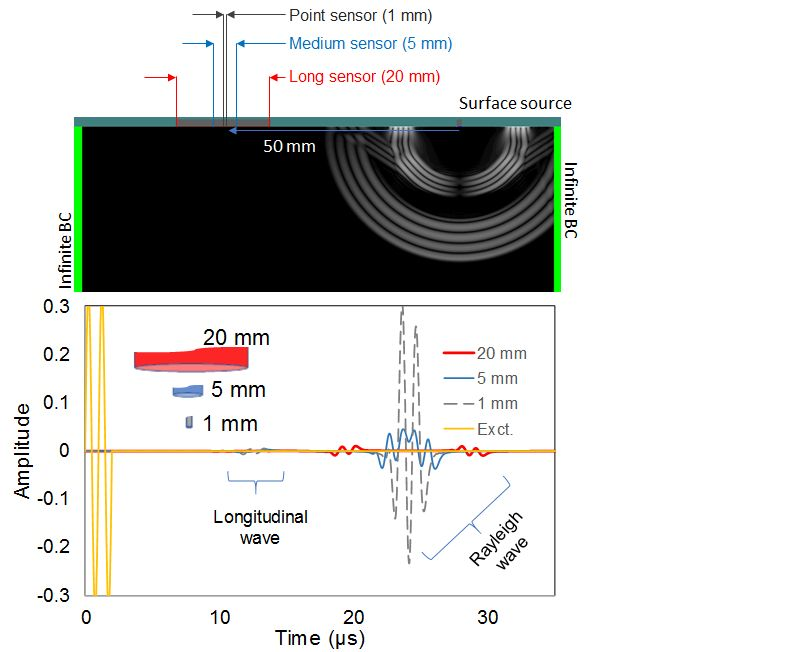
The simulated two-dimensional geometry is given in Figure 1. The physical properties were chosen close to concrete: longitudinal wave velocity 4300 m/s, shear velocity 2350 m/s and density 2300 kg/m3. Concrete was chosen as the most representative example of widely applied structural material used in bulk geometries, as metals and composites are usually formed in plates and the propagation conditions differ.
Three receivers with different size were used, namely 20 mm (called “long” sensor), 5 mm (“medium” sensor) and 1 mm (“point” sensor). The receiver sizes are chosen to simulate the commonly used sensors in AE field, while the smallest sensor of 1 mm was used as a reference. The receivers are set at the top side of the geometry shown in grey color in Figure 1.
The acoustic source was placed 50 mm away from the receivers at three different positions: on the surface, vertically beneath the receiver and diagonally (Figure 1). Under this configuration, the effect of the directionality of the source can also be assessed. The source was 1 mm long and produced a vertical displacement along its length. An actual source of AE is considered as a step function, thus very short in time, governed by the movement of the crack front (and the related oscillation around the new equilibrium position) [20]. The basic excitation was selected as two cycles of five different frequencies, namely 1 MHz, 500 kHz, 200 kHz, 100 kHz and 50 kHz aiming to cover large range of wavelengths. A discussion on the influence of the excitation duration is also included later. The simulated time was up to 100 µs resulting in a waveform length of 5194 samples and a sampling interval of 0.01925 µs or inversely sampling rate of 52 MHz. The space resolution was 0.1 mm, which was quite dense even for the case of highest frequency of 1 MHz with Rayleigh wavelength 2.35 mm.
3. Results
3.1. Surface Excitation
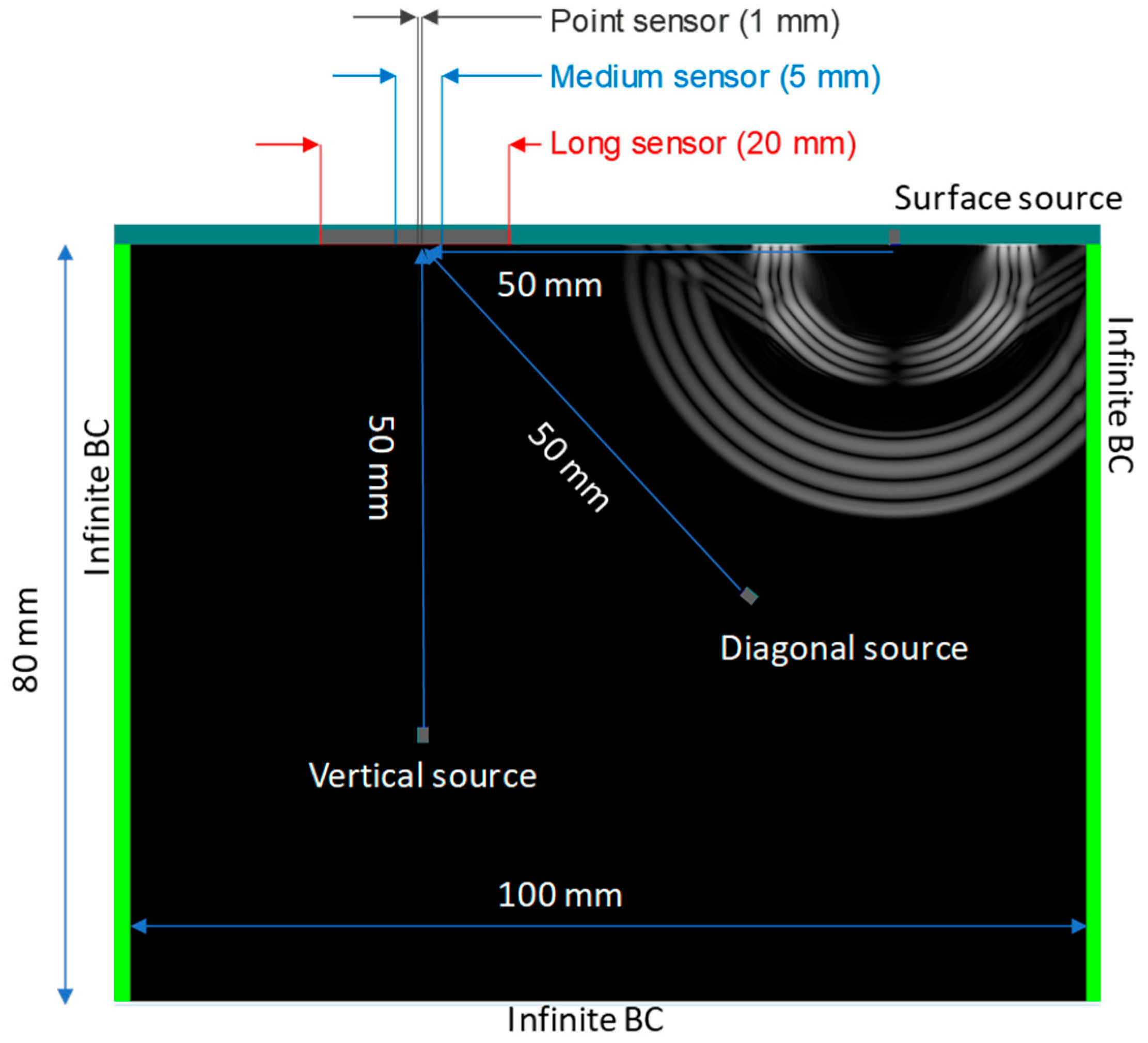
Results analysis begins with the waveforms received due to surface excitation since it exhibits the highest interest in the sense that the response of the different sensors exhibits strong variations. Figure 2 shows the excited signal (two cycles sinusoid in yellow color at the start of the time axis) and the respective waveforms received by each sensor in the case of 1 MHz excitation frequency. The units of amplitude are arbitrary as they concern the linear regime. If the displacement source waveform peaks at 1, it can be considered that the maximum source displacement is 1 μm. After the initial longitudinal wave arrivals noticed just after 15 µs, the considerably stronger Rayleigh wave arrives. The higher Rayleigh amplitude is expected as this wave mode occupies the highest amount of energy after a surface excitation (approximately 67%, while only around 7% forms the longitudinal) [21].
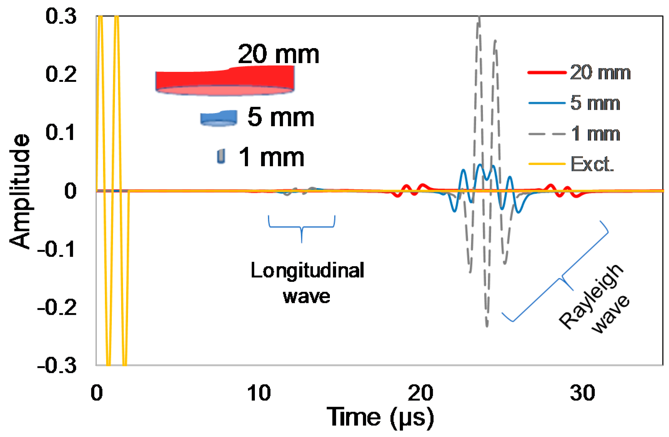
The “point” sensor (1 mm) registers quite clearly two strong cycles similar to the excited signal. However, the long sensor (20 mm) records a significantly distorted waveform: it consists of four small cycles interrupted by a plateau of nearly zero displacement. Looking at the displacement field of Figure 3a, corresponding to 22 µs after excitation, the Rayleigh wave packet is entirely on the sensor line, creating a cancellation effect due to positive and negative peaks acting simultaneously. The Rayleigh wavelength of 1 MHz is 2.35 mm, while the length of two cycles is 4.70 mm, which is much smaller than the sensor size (20 mm). It is seen that if the entire wave packet is within the physical limits of the sensor, cancellation effect of the total output occurs. In contrast, this is not the case for the point sensor (1 mm) as a single wavelength cannot fit into the sensor size. The received waveform shape follows the peaks and valleys of the excited wave packet reaching higher amplitudes than the long sensor case. The waveform received by the medium sensor (5 mm) has mixed characteristics consisting of approximately 5 cycles of amplitude in between the other two cases. From a general assessment, it is obvious that the smaller the physical dimension of the sensor (respectively the line along which averaging is conducted), the higher the similarity between the excited and received waveform.
Differences are strong in the frequency domain as well, as seen in Figure 3b where the Fast Fourier Transforms (FFT) of the waveforms of Figure 2 are shown. Only the response of point sensor (1 mm) exhibits similarities to the actual FFT of the excited signal, with a clear higher peak at around 1 MHz. The responses of medium (5 mm) and long (20 mm) sensors neither have resemblance to the excited signal nor show strong content around 1 MHz. It is characteristic that the initial excited content centered around 1 MHz is distributed approximately evenly to the whole range of the first MHz for the long sensor.
For AE damage characterization purposes, the latter observations are of utmost importance since the source excitation may be sensed by a severely distorted waveform on the receiver. The effect of sensor size modifies the output and influences the accuracy of the AE signal features and waveform shape in general. For lower frequencies, the differences in all aspects (waveform shape, FFTs) on sensors’ response to horizontal surface source diminish and are minimized for the excitation frequency of 50 kHz (respective wavelength equal to 48 mm). Indicative waveforms are shown in Figure 4a. The longest sensor (20 mm) still registers the lowest amplitude, but the difference is much smaller in this case while the waveform shape is very close to the one of point sensor. The FFTs show closer results as revealed in Figure 4b.
3.2. Vertical Excitation Beneath the Sensor
In the case of vertical excitation beneath the sensor, the study concerns the longitudinal wave since Rayleigh is not directly created from the excitation within the material. The simulation waveforms are shown in Figure 5a. The differences at the waveforms received by different size sensors are almost negligible. It should be noted that the amplitude of the signal received by long sensor (20 mm) is slightly lower than the waveforms of the other two cases. Additionally, the point and medium sensors’ waveforms begin slightly sharper than the corresponding of long sensor. This is due to the circular shape of the wave front that affects the wave arrival. More specifically, wave energy arrives vertically to the long sensor only in its center, but part of the energy arrives in slightly different angles at the sensors edges due to spreading. The above agrees with recent literature, stating that when the sensor diameter increases, the displacement distribution along the diameter becomes non-uniform [22]. This is not the case for smaller size sensors at which the whole energy arrives vertically and the wave front shape effect is negligible. The differences are minimized for lower frequencies with the example of 50 kHz in Figure 5b being indicative.
3.3. Diagonal Excitation
Diagonal wave propagation provides an intermediate response between the vertical and the surface cases, but strong differences can still be observed. Figure 6a shows the waveforms received by each sensor in the case of 1 MHz excitation frequency. The early strong burst originates from the longitudinal wave impinging on the sensors at an angle of 45°. This angle is also the reason of the lower amplitude (up to 0.2 peak to peak for the point sensor) compared to longitudinal waves of vertical source excitation (amplitude higher than 0.5, Figure 2). Once again, the waveform of the long sensor (20 mm) significantly differs from the excited signal (sinusoid of two cycles) due to the aforementioned cancellation effect. As shown in Figure 6a, at approximately 20 μs, a second wave packet arrives attributed to the slower shear wave front which is detected due to the angle of incidence.
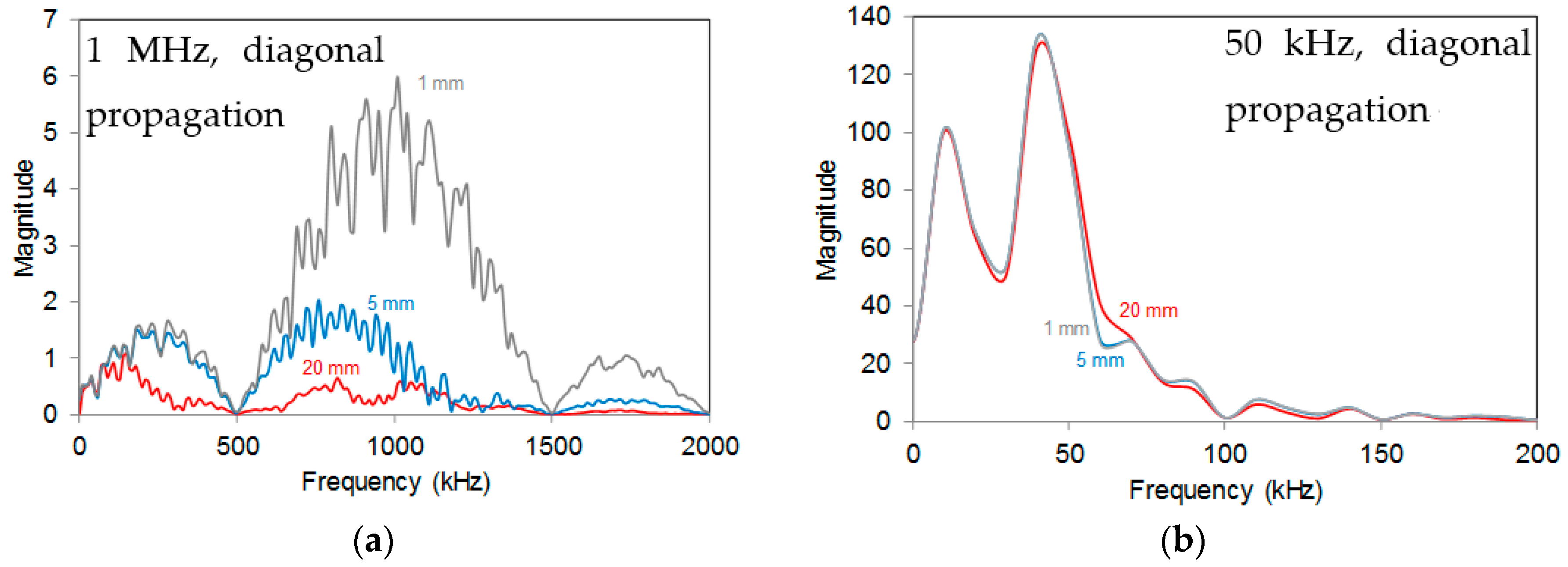
Respectively, in Figure 7a,b the FFTs of waveforms received by different size sensors in the extreme cases of 1 MHz and 50 kHz are shown. Strong differences from the original FFT envelope are observed in the case of 1 MHz excitation, especially by long and medium sensors attributed to the cancellation effect (Figure 7a). On the contrary, in the case of 50 kHz excitation frequency (Figure 7b), the FFT functions of three size sensors are almost identical converging to the same curve.
4. Discussion
4.1. Impact of Sensor Size on Signal Amplitude
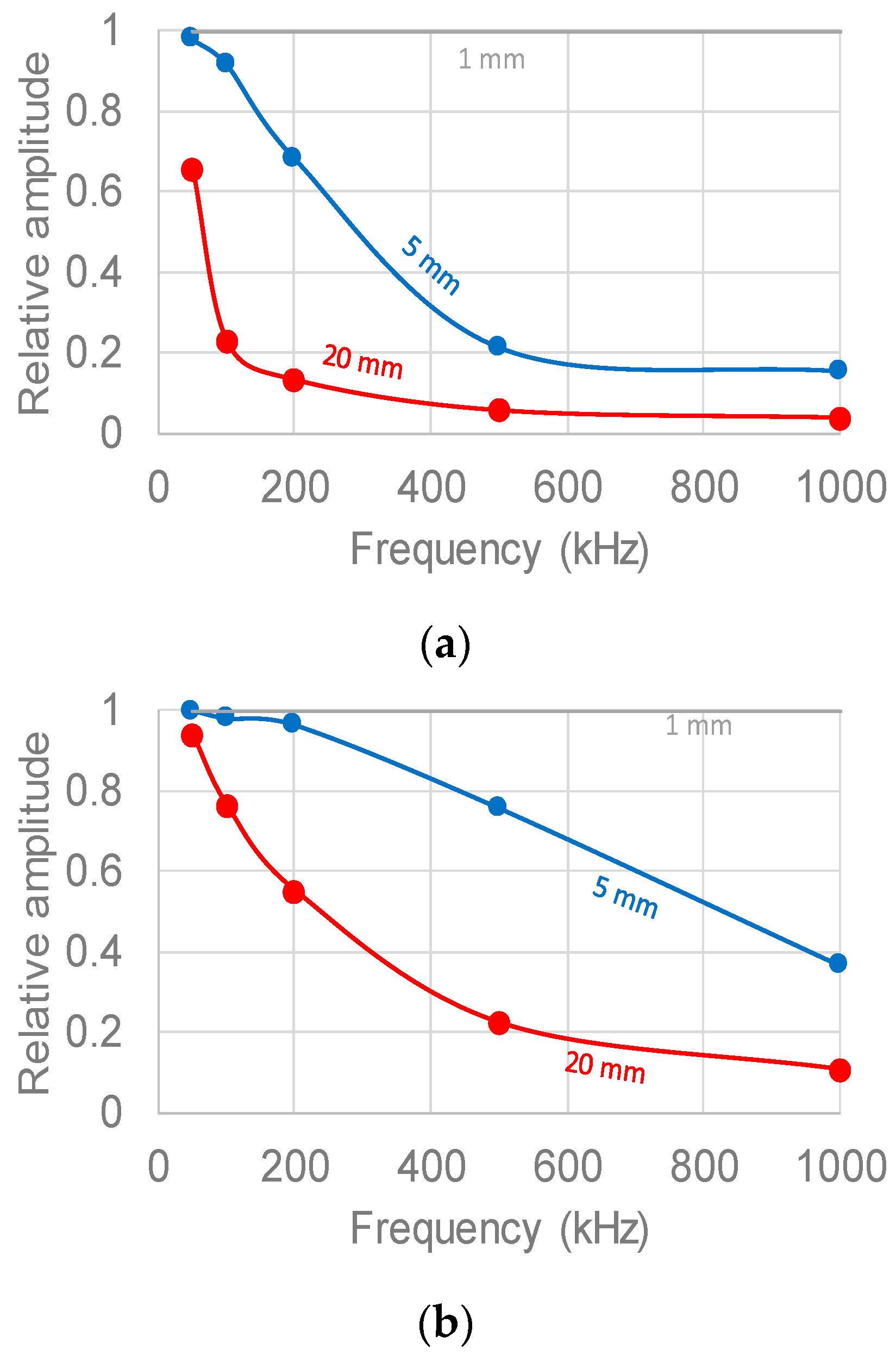
The effect of sensor size on signal response is quantified considering the amplitude of the signal received by different size sensors normalized over the amplitude of the point sensor which is considered as reference. The relative amplitude values are presented in Figure 8 for all three source directions and covering the frequency range from 50 kHz to 1 MHz.
In the surface wave propagation case (Figure 8a) and for high frequencies (up to 1 MHz), the output of the larger sensors is just a fraction of the response of the point sensor. Specifically, considering the long sensor (20 mm), the relative amplitude is equal to 3.6% of the reference. Moving towards lower frequencies, the relative amplitude is gradually restored, earlier for the medium and then for the long sensor. At 50 kHz, the relative amplitude of the long sensor is still around 0.65 indicating that even at low frequencies the signal remains significantly distorted.
In the diagonal wave propagation case (Figure 8b), the medium sensor seems to approach the point sensor response especially at low excitation frequency ranges (from 50 to 200 kHz). This is not the case for the long sensor that receives a much lower amplitude. Indicatively, at 500 kHz excitation frequency, the amplitude of the long sensor is just 22% of the point sensor, while for 200 kHz it is just above 54%.
Concerning the last case, where the source is placed vertically beneath the receiver (Figure 8c), relative amplitude is much closer to unity (difference between point sensor and long sensor at 1 MHz excitation frequency is about 15%). These results indicate that the sensor size effect is minimized for propagation vertical to the sensor surface in contrast to other angles of incidence.
It is concluded that sensor size effect dominantly influences the received waveform shape in almost the whole frequency range and especially when the source does not stand directly beneath the sensor. As expected, the measurements obtained by AE on bulk materials, such as concrete where stochastic defects are included, carry an error due to sensor size effect and may provide less accurate signal amplitude. In real size structures, wave attenuation eliminates the higher frequencies, but still frequencies up to 200 kHz are commonly measured, therefore the signal amplitude can be affected by the sensor size. However, in tests done in laboratory, even higher frequencies are measured meaning that the influence of the sensor effect will be even stronger.
4.2. Effect of Wavelength over Sensor Size
The case of surface waves obviously exhibits the strongest aperture effect. To quantify the trends, the amplitude data are presented in terms of the normalized parameter D/λ (sensor size over wavelength) in Figure 9. The individual curves follow a «master curve», stressing that the crucial parameter is the ratio of sensor size/wavelength. This curve can be well fitted by an exponential function. As the sensor size increases away from the ideal case of “point” sensor, the relative amplitude sharply decreases until the point D/λ 1 when the sensor size is equal to the wavelength. At that point, the relative amplitude has already dropped to 20% of the reference. For larger sensor size, the amplitude decreases further but with a lower rate reaching 4% for D/λ > 8.
4.3. Impact of Sensors Size Effect on Frequency Content
The sensor size effect does not only influence the amplitude but also the wave shape in both time and frequency domain. Considering the frequency content, the most crucial measure of the similarity between two waveforms (X(t), Y(t)) is the “coherence function, γxy”. This function is given by:
where: and , are the autospectral density functions of X(t) and Y(t) respectively and is the cross-spectral density function between X(t) and Y(t). Coherence is analogous to the squared correlation coefficient of time domain functions underlying the frequency similarities of the signals [23]. In case of identical emitted and received waveforms, coherence gets a unity value. Coherence has also been measured to classify AE [24] and acousto-ultrasonics signals [25] based on their similarity to reference waveforms. In this case it was calculated based on a standard Matlab function. The waveforms were zero-padded to the length of 32,768 points while the required overlap window was 1250 points. These settings were constant for all calculations below but are not unique and could be changed leading to a somehow different final function.
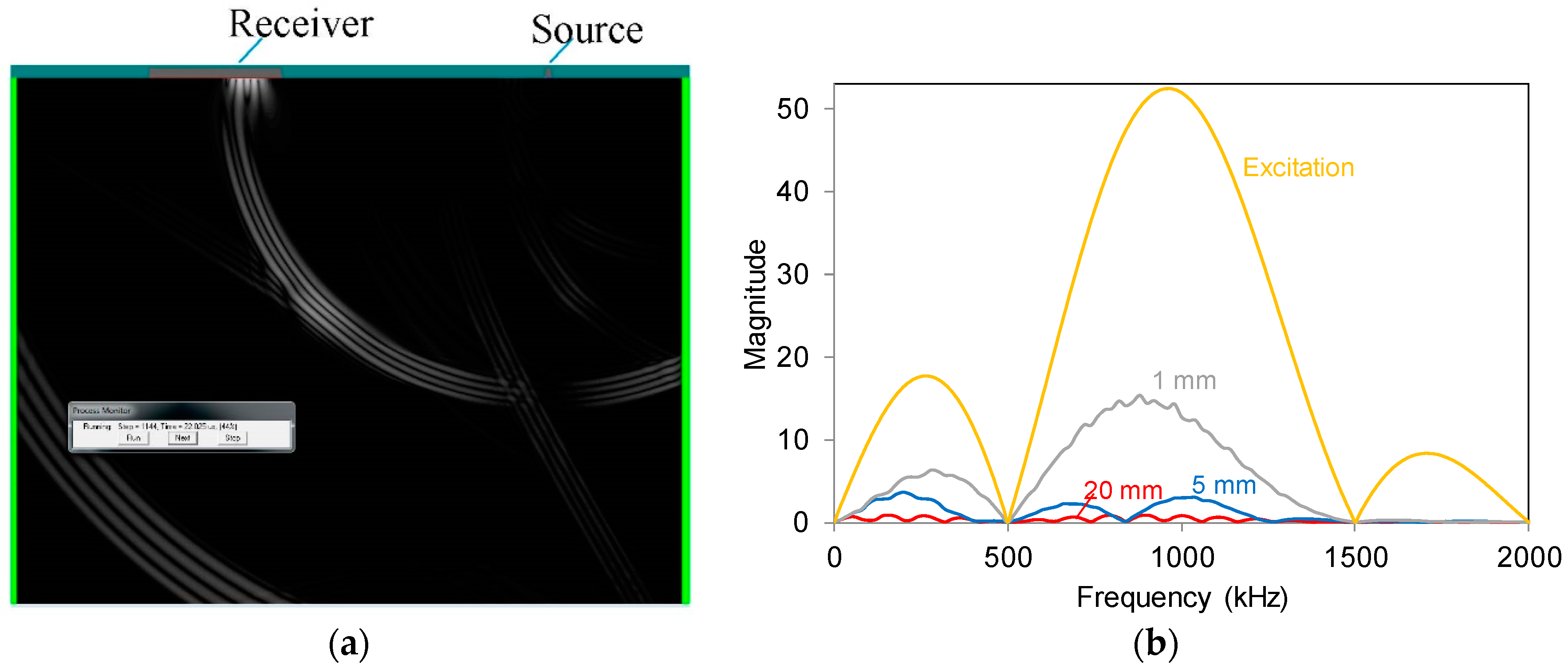
Figure 10a shows indicatively the wave emitted with excitation frequency at 1 MHz (in red), and the waveforms received by the medium sensor (5 mm) for the cases of source set on the surface (in black) and vertically beneath the sensor (in blue). It is shown that the similarity to the original wave is stronger for the vertically placed source, when two clear cycles are depicted, while for the case of surface waves, the major content of the Rayleigh waves shows four to five cycles instead of two. Figure 10b shows the corresponding coherence functions between the received waveforms and the excitation up to 2 MHz. The level of coherence is much higher for the direct propagation vertical to the sensor where the function is almost constantly close to unity, indicative of excellent similarity between the excitation and the sensor output. On the other hand, the coherence function of surface waves has significantly lower values with an average around 0.6 indicative of strong distortion that affects the received waveform.
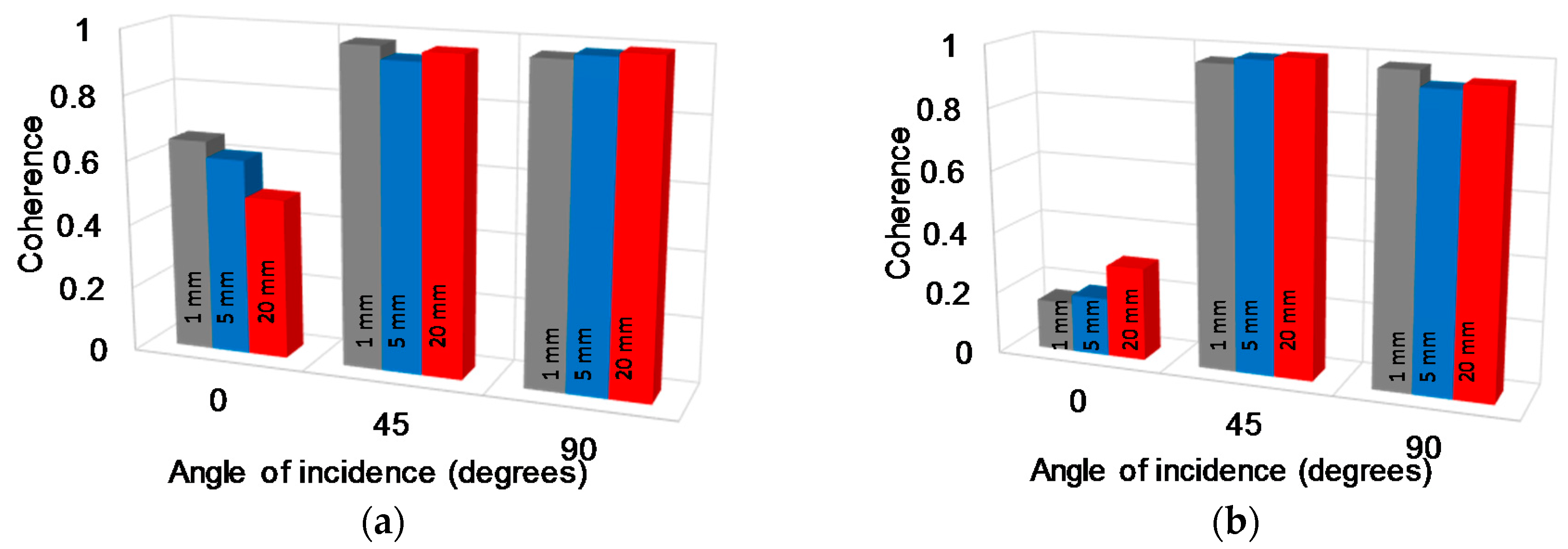
The average level of coherence between the excitation and the received signal is shown in Figure 11 for the different angles of incidence and the various sensors sizes for two indicative excitation frequencies (a) 1 MHz and (b) 500 kHz. For the case of 1 MHz the coherence is quite high (more than 95%) for diagonal and vertical to the sensor surface propagation for all sensors. However, for propagation parallel to the surface (angle 0°), coherence is lower. Still, again the point sensor yields higher values (0.66) compared to the longer sensor (0.49). For the surface propagation of 500 kHz (case b), coherence is very low (below 0.3) showing a huge amount of distortion on the frequency content for all sensors, while it is again close to unity for diagonal and vertical direction of incidence. The above coherence analysis indicates that the received signal is crucially distorted in spectral content for surface propagation meaning that sources on or close to the surface will exhibit lower spectral similarity to the finally obtained waveform than a source at the same distance beneath the sensor. The latter should be considered in studies that use sensors calibrated in face-to-face configurations to assess the response of waveforms that travel on the material’s surface.
4.4. Experimental Evidence
Experimentally, the sensor size effect cannot be directly compared between two different sensors, since apart from their possible difference in size or surface contact area, they also possess different frequency response characteristics. In addition, in the specific case studied herein, results between simulations and experiments cannot be directly compared for a number of reasons. First, the damping of the material is not readily known like other parameters (e.g., the elastic modulus) to be imported in the simulation. In addition, although a numerical source can be excited within the material to introduce a pure longitudinal wave, this cannot be realized experimentally as the excitation takes place on the surface forming again stronger Rayleigh waves. Therefore, it is reasonable to compare simulated and experimental waveforms after excitation on the same surface (case of horizontal propagation above) but there is no straightforward quantitative comparison for the case of vertical propagation.
However, there is one point of interest which shows the strength of the sensor size effect. As mentioned above, when excitation takes place on the surface, 67% of the energy forms the Rayleigh wave. On the other hand, experimentally, the only amount of energy captured by the sensor standing at the opposite side is the 7% of the longitudinal wave. Therefore, it is expected that the horizontal propagation case will result in stronger waveform than the vertical, also because Rayleigh waves suffer less geometric spreading. Numerically, this is shown when comparing the waveform received by the point sensor coming from the surface excitation (Figure 2, with peak to peak amplitude higher than 0.5) and vertical excitation (Figure 5a, respective amplitude range 0.3). The response to surface excitation is much higher due to the strength of the Rayleigh wave and the reduced geometric spreading of the beam.
In this direction, experimental measurements with pencil lead breakage (Hsu-Nielsen source) as acoustic source were conducted (Figure 12). A receiver sensor was positioned at the top surface of a normal strength concrete sample. The sample had 50 mm thickness. Pencil lead breakages were performed at 50 mm far from the receiver at the top surface and at the bottom side of the sample, just beneath the receiver, as shown in Figure 12.
The above experimental arrangement was realized using two types of AE sensors. One is the widely used in practice “R15” of Mistras Group with a sharp resonant peak at 150 kHz and diameter of 19 mm. The other is the “Pico” of the same manufacturer with a broader response and much smaller diameter of 5 mm. A pre-trigger capturing time of 50 μs was used. The sampling rate was 2 MHz and the pre-amplification gain was 40 dB.
Figure 13 shows several waveforms, each one corresponding to an individual pencil lead break, recorded by vertical (a) and surface horizontal (b) propagation recorded by the Pico (5 mm) sensor. The waveforms are quite repeatable especially at the early part that contains the so-called “ballistic” pulse which is not much influenced by scattering [26]. Visually, the waveforms from the surface excitation (Figure 13b) obtain higher amplitude in average than the ones of vertical excitation (Figure 13a). Measuring the peak-to-peak absolute voltage of the highest cycle of the waveforms, the average for the horizontal ones is 0.84 V while for the vertical the average amplitude is 0.54 V. This is verified by the higher peak of the FFT curve of the surface horizontal wave shown in Figure 13c. The FFT curves presented here are obtained by averaging the individual FFTs of waveforms in Figure 13a,b respectively.
In contrast, using the longer sensor R15 (19 mm), the waveforms from vertical orientation are higher than surface (Figure 14a,b respectively). Specifically, the peak-to-peak absolute amplitude for vertical averages at 6.88 V while for the horizontal propagation this is 5.81 V. The FFT curves of Figure 14c confirm this trend, showing higher magnitude for the vertical excitation case compared to the horizontal surface excitation. The data imply that the sensor size effect influences the surface propagation leading to a received wave magnitude decrease, even though physically surface waves are stronger than longitudinal.
The main content of the FFT curve (Figure 14c) is positioned around 150 kHz. Considering this frequency, the Rayleigh wavelength is calculated at around 16 mm, a value similar to the R15 sensor size (19 mm) and three times greater than the Pico size (5 mm). It is shown that considering the same propagation distance and for sensor physical size similar to the wave length (case of R15), the aperture effect diminishes the Rayleigh wave magnitude to levels lower than the corresponding longitudinal of the vertical excitation. However, for a smaller sensor, the Rayleigh wave magnitude remains higher than the corresponding longitudinal impinging vertically. This is confirmed in recent literature, in which the sensitivity of specific AE sensors was measured against both vertically incident and bar waves propagating parallel to the sensor surface. For various sensors, the sensitivity to parallel waves was lower than the sensitivity to vertical waves as the frequency increased [16]. It is characteristic that concerning sensor “R6” of Mistras, the sensitivity curves start to deviate at approximately 300 kHz, corresponding to a diameter over wavelength ratio of approximately 0.5 (element size according to [16] is 12.7 mm and the wavelength on reference aluminum bar for this frequency is approximately 22 mm). This agrees with the presented master curve of Figure 9, where the relative amplitude has high values only for D/λ < 0.5. Furthermore, in another study related to surface wave measurements, it is stated that the optimal operation frequency of the sensor is when the aperture size is no longer than half or even a quarter of the wavelength [27].
5. Secondary Effects
The influence of the pulse length or waveform duration is also of interest as it results in a different physical waveform length acting on the sensor’s surface. This should not be confused with the wave length which is the wave parameter defined as propagation velocity over frequency. To examine the influence of the waveform duration (i.e., short vs. long signal of the same basic frequency), surface wave simulations were repeated for different number of excitation cycles (from 1 to 20). Two cases of excitation frequencies and sensor sizes were applied, i.e., 1 MHz (wavelength λ = 2.35 mm) with 5 mm sensor size and 500 kHz (λ = 4.7 mm) with 20 mm sensor size. For both cases, one cycle of excitation produces a wavelength smaller than the sensor size, while adding more cycles results eventually in a total wave longer than the sensor size. Indicative waveforms for frequency of 500 kHz received by the 20 mm size sensor for 1 and 10 cycles of excitation are shown in Figure 15a.
As the waveform becomes longer, the received peak amplitude increases (see Figure 15a). There is a characteristic point at which a jump in amplitude is observed. This is when the total wave length becomes equal to the sensor size, as seen in Figure 15b. In this figure, the amplitude for each curve is normalized to maximum, while the horizontal axis measures the total waveform length (number of cycles times the wave length) over the sensor size. Therefore, it is seen that the duration of a waveform has an indirect effect on the measured amplitude since when its length becomes equal or longer than the sensor, it can increase the latter by approximately 35%. This influence of waveform length (pulse length) over sensor size is noticeable in the simulation but is not as strong as the wavelength over size influence that was presented in Figure 9. In addition, for experimental waveforms which usually do not have constant amplitude cycles this effect would be weaker due to lower level of constructive interference.
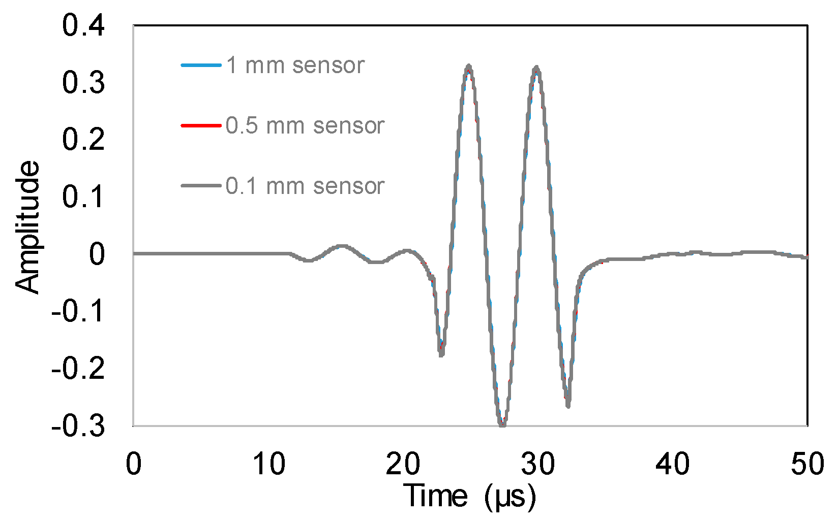
The minimum sensor size used in this study as reference was 1 mm. Although this is not exactly a “point”, or infinitesimally small sensor, the results do not deviate significantly for the casual AE wavelengths. Figure 16 shows the simulated received waveforms for sensors of 1 mm, 0.5 mm and 0.1 mm after a surface excitation of 200 kHz which is typical for AE in concrete.
The waveforms are literally identical without distortion on the shape or the peak to peak amplitude. Therefore, considering that element sizes smaller than 1 mm are not commonly used in AE practice, the sensor of 1 mm was considered as reference.
A further point that should be kept in mind is related to the dispersion phenomenon. This study focuses on a homogeneous bulk material and monochromatic frequency in order to quantify the sensor size effect. Different cases of media can be considered in the future, like the case of heterogeneous bulk material, where scattering dispersion may impose a frequency dependent velocity as well as the case of thin plates where dispersion originates from the geometry (plate wave dispersion). In these cases, the pulse would spread in time domain altering the duration and the contact time with the sensor. Another interesting case is of anisotropic media where velocity (and thus wavelength) changes with direction, typical of composite plates. There the “aperture” effect would change for different directions depending on the orientation of the fibres.
6. Conclusions
Although the sensor size effect is acknowledged in wave propagation studies, it is rarely quantified. Herein, the sensor size effect is numerically assessed for AE wave propagation in concrete and different angles of incidence to the surface. Simulations enable the isolation of the size effect without influence from the frequency response of the piezoelectric element. It is shown that the small physical size of sensor enables more precise representation of the actual propagating wave. Concerning Rayleigh waves that present the strongest aperture effect, the results can be expressed in terms of the sensor size over wavelength parameter. As this ratio increases from zero (the ideal case of point sensor) to 0.5, the amplitude has already lost approximately 35% and when the wavelength becomes equal to the sensor, the amplitude has lost 80% of the amplitude of a point sensor. For longer sensors relative to the wavelength, the amplitude continues to decrease with a smoother slope. Coherence analysis conducted between the received and original waves shows that waveforms received from surface propagating waves carry stronger distortion compared to longitudinal waves emitted from a source into the material standing diagonally or vertically beneath the sensor. Experimental evidence was taken using two widely applicable sensors. The smaller size sensor records the Rayleigh wave on the surface with higher amplitude than the longitudinal impinging vertically emitted by source located at the opposite side of a concrete sample and at the same distance. The result is inverse for a larger sensor, being a clear manifestation of the sensor size effect. The latter indicates that the amplitude of sources near the surface are more prone to underestimation errors when a large sensor size is used. Frequency content of the received waves is also distorted due to the sensor size, increasing the possible distortion due to scattering or reflections.
Acknowledgments
Financial support of the Research Foundation Flanders (FWO-Vlaanderen, Project No 28976) for this study is gratefully acknowledged.
Author Contributions
Dimitrios G. Aggelis conceived, designed and performed the numerical simulations; Eleni Tsangouri performed the experiments and analyzed the data; Dimitrios G. Aggelis and Eleni Tsangouri wrote the paper.
Conflicts of Interest
The authors declare no conflict of interest.
References
- Prosser, W.H. Acoustic Emission. In Nondestructive Evaluation, Theory, Techniques and Applications; CRC Press: New York, NY, USA, 2002; pp. 369–446. ISBN 9780824788728. [Google Scholar]
- Ishibashi, A.; Matsuyama, K.; Alver, N.; Suzuki, T.; Ohtsu, M. Round-robin tests on damage evaluation of concrete based on the concept of acoustic emission rates. Mater. Struct. 2016, 49, 2627–2635. [Google Scholar] [CrossRef]
- Sagasta, F.; Benavent-Climent, A.; Roldán, A.; Gallego, A. Correlation of Plastic Strain Energy and Acoustic Emission Energy in Reinforced Concrete Structures. Appl. Sci. 2016, 6, 84. [Google Scholar] [CrossRef]
- Shiotani, T.; Oshima, Y.; Goto, M.; Momoki, S. Temporal and spatial evaluation of grout failure process with PC cable breakage by means of acoustic emission. Constr. Build. Mater. 2013, 48, 1286–1292. [Google Scholar] [CrossRef]
- Carpinteri, A.; Xu, J.; Lacidogna, G.; Manuello, A. Reliable onset time determination and source location of acoustic emissions in concrete structures. Cem. Concr. Compos. 2012, 34, 529–537. [Google Scholar] [CrossRef]
- Tsangouri, E.; Karaiskos, G.; Deraemaeker, A.; Van Hemelrijck, D.; Aggelis, D.G. Assessment of acoustic emission localization accuracy on damaged and healed concrete. Constr. Build. Mater. 2016, 129, 163–171. [Google Scholar] [CrossRef]
- Shahidan, S.; Pullin, R.; Bunnori, N.M.; Holford, K.M. Damage classification in reinforced concrete beam by acoustic emission signal analysis. Constr. Build. Mater. 2013, 45, 78–86. [Google Scholar] [CrossRef]
- Farhidzadeh, A.; Salamone, S.; Singla, P. A probabilistic approach for damage identification and crack mode classification in reinforced concrete structures. J. Intell. Mater. Syst. Struct. 2013, 24, 1722–1735. [Google Scholar] [CrossRef]
- Blom, J.; El Kadi, M.; Wastiels, J.; Aggelis, D.G. Bending fracture of textile reinforced cement laminates monitored by acoustic emission: Influence of aspect ratio. Constr. Build. Mater. 2014, 70, 370–378. [Google Scholar] [CrossRef]
- McLaskey, G.C.; Glaser, S.D. Acoustic Emission Sensor Calibration for Absolute Source Measurements. J. Nondestruct. Eval. 2012, 31, 157–168. [Google Scholar] [CrossRef]
- Ono, K. Acoustic Emission in Materials Research—A Review. J. Acoust. Emiss. 2011, 29, 284–308. [Google Scholar]
- Zelenyak, M.; Hamstad, M.A.; Sause, M.G. Modeling of acoustic emission signal propagation in waveguides. Sensors 2015, 15, 11805–11822. [Google Scholar] [CrossRef] [PubMed]
- To, A.C.; Glaser, S.D. Full waveform inversion of a 3-D source inside an artificial rock. J. Sound Vib. 2005, 285, 835–857. [Google Scholar] [CrossRef]
- Ono, K. Calibration Methods of Acoustic Emission Sensors. Materials 2016, 9, 508. [Google Scholar] [CrossRef] [PubMed]
- Ono, K. On the Piezoelectric Detection of Guided Ultrasonic Waves. Materials 2017, 10, 1325. [Google Scholar] [CrossRef] [PubMed]
- Ono, K.; Hayashi, T.; Cho, H. Bar-Wave Calibration of Acoustic Emission Sensors. Appl. Sci. 2017, 7, 964. [Google Scholar] [CrossRef]
- Sause, M.G.R.; Hamstad, M.A.; Horn, S. Finite element modeling of conical acoustic emission sensors and corresponding experiments. Sens. Actuators A Phys. 2012, 184, 64–71. [Google Scholar] [CrossRef]
- Sause, M.G.R.; Hamstad, M.A. Numerical modeling of existing acoustic emission sensor absolute calibration approaches. Sens. Actuators A Phys. 2018, 269, 294–307. [Google Scholar] [CrossRef]
- Wave2000®/Wave2000® Plus-Software for Computational Ultrasonics. Available online: http://www.cyberlogic.org/wave2000.html (accessed on 15 October 2017).
- Pollock, A.A. Acoustic emission-2: Acoustic emission amplitudes. Non-Destr. Test. 1973, 6, 264–269. [Google Scholar] [CrossRef]
- Graff, K.F. Wave Motion in Elastic Solids; Dover Publications: New York, NY, USA, 1975; p. 688. ISBN 978-04-8-666745-4. [Google Scholar]
- Zhang, L.; Yalcinkaya, H.; Ozevin, D. Numerical approach to absolute calibration of piezoelectric acoustic emission sensors using multiphysics simulations. Sens. Actuators A Phys. 2017, 256, 12–23. [Google Scholar] [CrossRef]
- Bendat, J.S.; Piersol, A.G. Engineering Applications of Correlation and Spectral Analysis; Wiley: New York, NY, USA, 1993; p. 472. ISBN 978-0-471-57055-4. [Google Scholar]
- Grosse, C.U.; Reinhardt, H.; Dahm, T. Localization and classification of fracture types in concrete with quantitative acoustic emission measurement techniques. NDT E Int. J. 1997, 30, 223–230. [Google Scholar] [CrossRef]
- Philippidis, T.; Aggelis, D.G. An acousto-ultrasonic approach for the determination of water-to-cement ratio in concrete. Cem. Concr. Res. 2003, 33, 525–538. [Google Scholar] [CrossRef]
- Cowan, M.L.; Beaty, K.; Page, J.H.; Liu, Z.; Sheng, P. Group velocity of acoustic waves in strongly scattering media: Dependence on the volume fraction of scatterers. Phys. Rev. E 1998, 58, 6626–6636. [Google Scholar] [CrossRef]
- Lee, Y.-C.; Kuo, S.H. A new point-source/point-receiver acoustic transducer for surface wave measurement. Sens. Actuators A Phys. 2001, 94, 129–135. [Google Scholar] [CrossRef]
Figure 1.
Simulation model geometry.

Figure 2.
Waveforms received by different size sensors for the case of surface source and excitation frequency of 1 MHz. The excitation wave (yellow starting at time 0) was reduced to the graph axes for clarity (nominal amplitude of 1).
Figure 2.
Waveforms received by different size sensors for the case of surface source and excitation frequency of 1 MHz. The excitation wave (yellow starting at time 0) was reduced to the graph axes for clarity (nominal amplitude of 1).

Figure 3.
(a) Snapshot of displacement field corresponding to 22 μs after excitation (frequency at 1 MHz). The source is set on the surface; (b) Fast Fourier Transforms (FFT) functions of the waveforms received by different size sensors.
Figure 3.
(a) Snapshot of displacement field corresponding to 22 μs after excitation (frequency at 1 MHz). The source is set on the surface; (b) Fast Fourier Transforms (FFT) functions of the waveforms received by different size sensors.

Figure 4.
(a) Waveforms received by different size sensors for the case of surface source and excitation frequency of 50 kHz; (b) FFT functions of waveforms received by different size sensors (exc. frequency at 50 kHz and surface source). The corresponding waveforms are depicted in Figure 4a.
Figure 4.
(a) Waveforms received by different size sensors for the case of surface source and excitation frequency of 50 kHz; (b) FFT functions of waveforms received by different size sensors (exc. frequency at 50 kHz and surface source). The corresponding waveforms are depicted in Figure 4a.
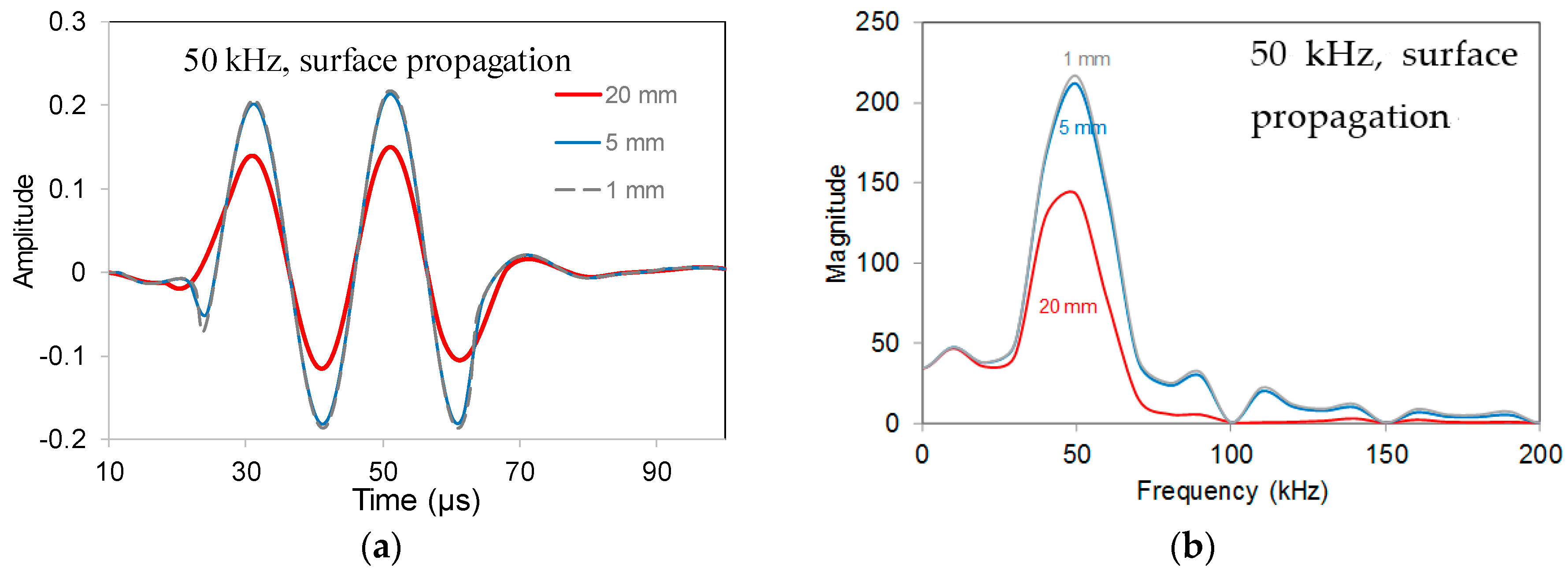
Figure 5.
(a) Waveforms received by different size sensors for the case of vertical source and excitation frequency of 1 MHz; (b) Waveforms received by different size sensors for the case of vertical source and excitation frequency of 50 kHz.
Figure 5.
(a) Waveforms received by different size sensors for the case of vertical source and excitation frequency of 1 MHz; (b) Waveforms received by different size sensors for the case of vertical source and excitation frequency of 50 kHz.

Figure 6.
(a) Waveforms received by different size sensors for the case of diagonal source and frequency excitation of 1 MHz; (b) Snapshot of displacement field corresponding to 10 μs after excitation (exc. frequency at 1 MHz).
Figure 6.
(a) Waveforms received by different size sensors for the case of diagonal source and frequency excitation of 1 MHz; (b) Snapshot of displacement field corresponding to 10 μs after excitation (exc. frequency at 1 MHz).
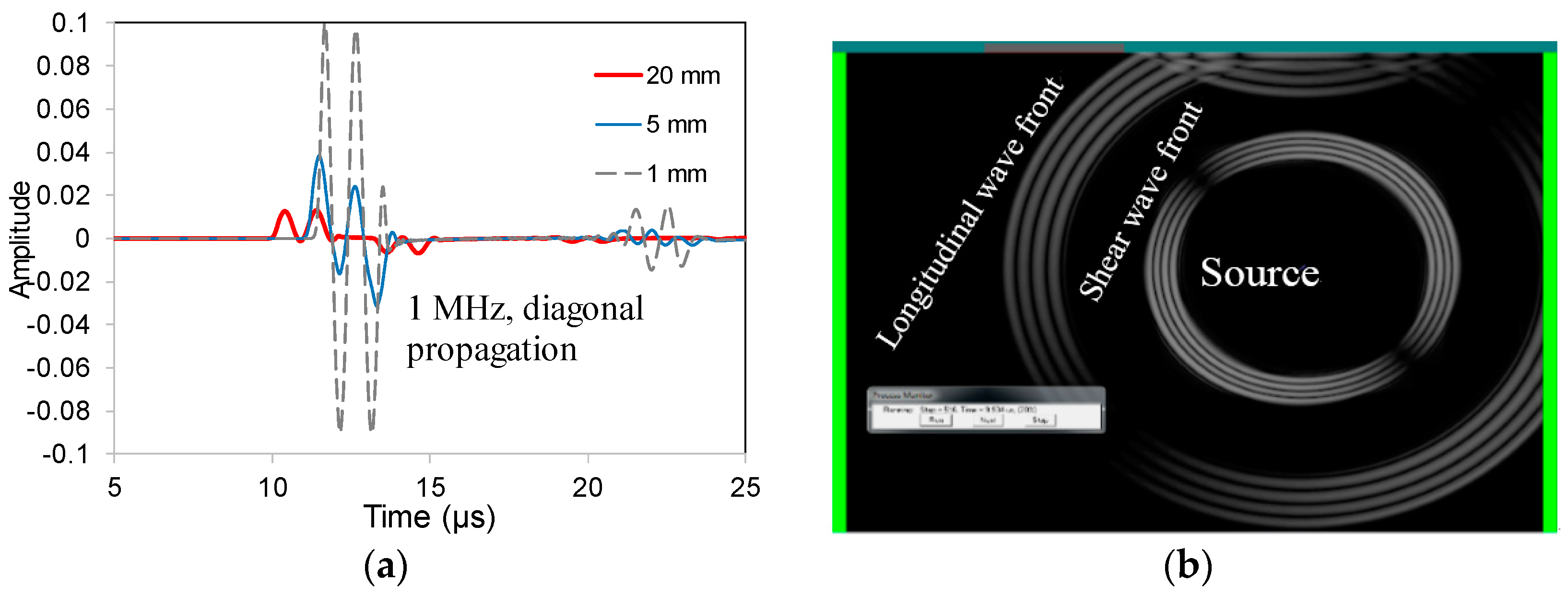
Figure 7.
(a) FFT functions of waveforms received by different size sensors (exc. frequency at 1 MHz and diagonal source); (b) FFT functions of waveforms received by different size sensors (exc. frequency at 50 kHz and diagonal source).
Figure 7.
(a) FFT functions of waveforms received by different size sensors (exc. frequency at 1 MHz and diagonal source); (b) FFT functions of waveforms received by different size sensors (exc. frequency at 50 kHz and diagonal source).

Figure 8.
Relative amplitude of the received signal for point (1 mm, in grey), medium (5 mm, in blue), long (20 mm, in red) along the frequency range, from 50 kHz to 1 MHz, and concerning the three source positions: (a) surface; (b) diagonal; (c) vertical.
Figure 8.
Relative amplitude of the received signal for point (1 mm, in grey), medium (5 mm, in blue), long (20 mm, in red) along the frequency range, from 50 kHz to 1 MHz, and concerning the three source positions: (a) surface; (b) diagonal; (c) vertical.

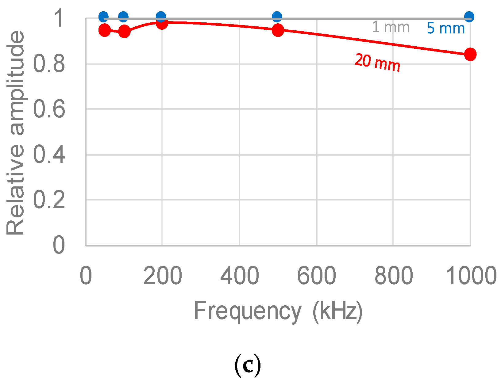
Figure 9.
Relative amplitude vs. sensor size over wavelength parameter (D/λ).
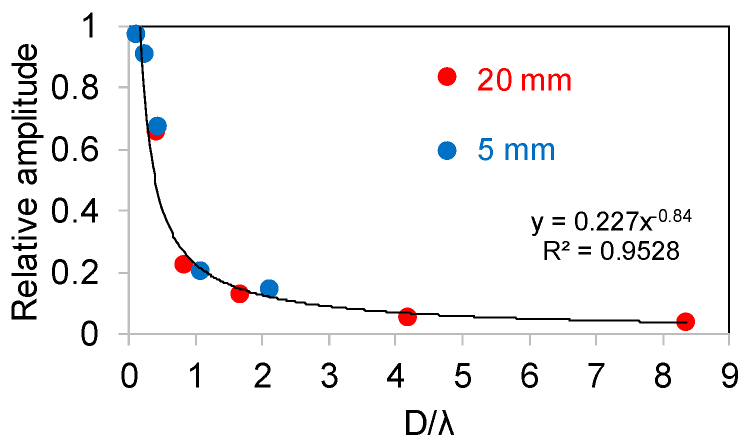
Figure 10.
(a) Waveforms received by the 5 mm size sensor emitted from source set on the surface (in black) and vertically beneath the sensor (in blue) with excitation frequency equal to 1 MHz. Original waveform is added in red color and in reduced scale to fit the graph; (b) Respective coherence functions between received waves and original.
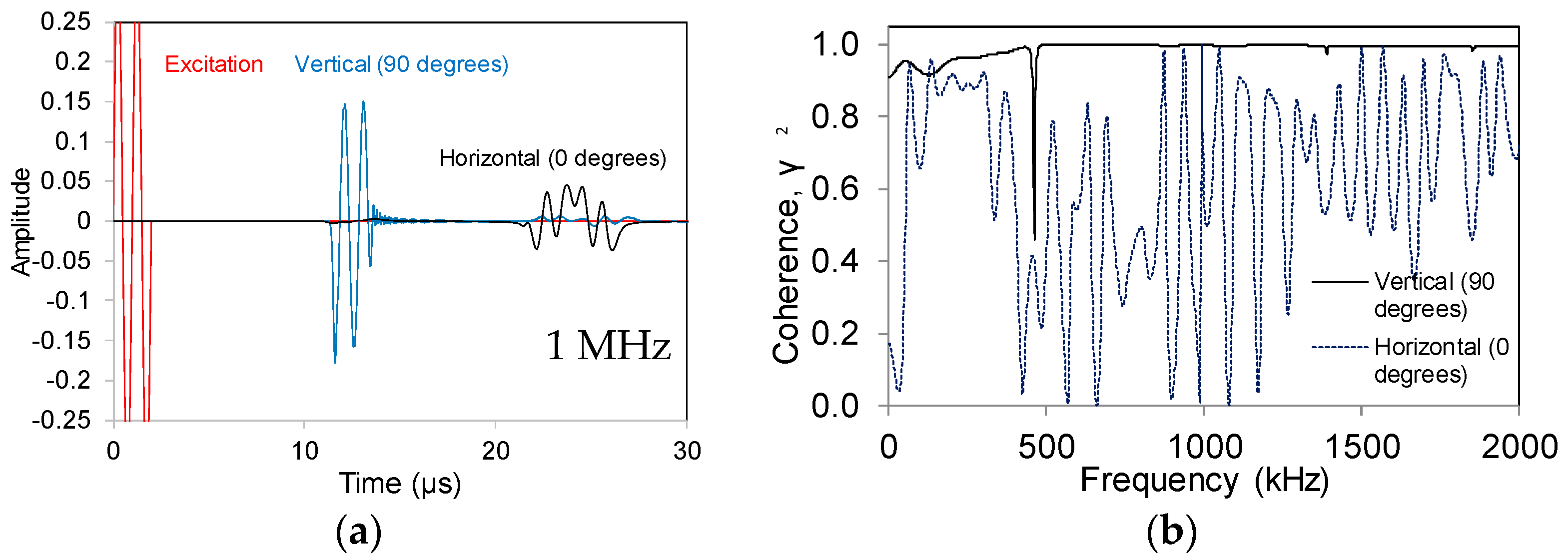
Figure 11.
Average coherence up to 2 MHz for different sensor size and angles of propagation relatively to the sensor surface and excitation frequencies (a) 1 MHz; (b) 500 kHz.
Figure 11.
Average coherence up to 2 MHz for different sensor size and angles of propagation relatively to the sensor surface and excitation frequencies (a) 1 MHz; (b) 500 kHz.

Figure 12.
Experimental setup showing the receiver at the top concrete surface and pencil lead breakage applied at the horizontal and vertical direction.
Figure 12.
Experimental setup showing the receiver at the top concrete surface and pencil lead breakage applied at the horizontal and vertical direction.
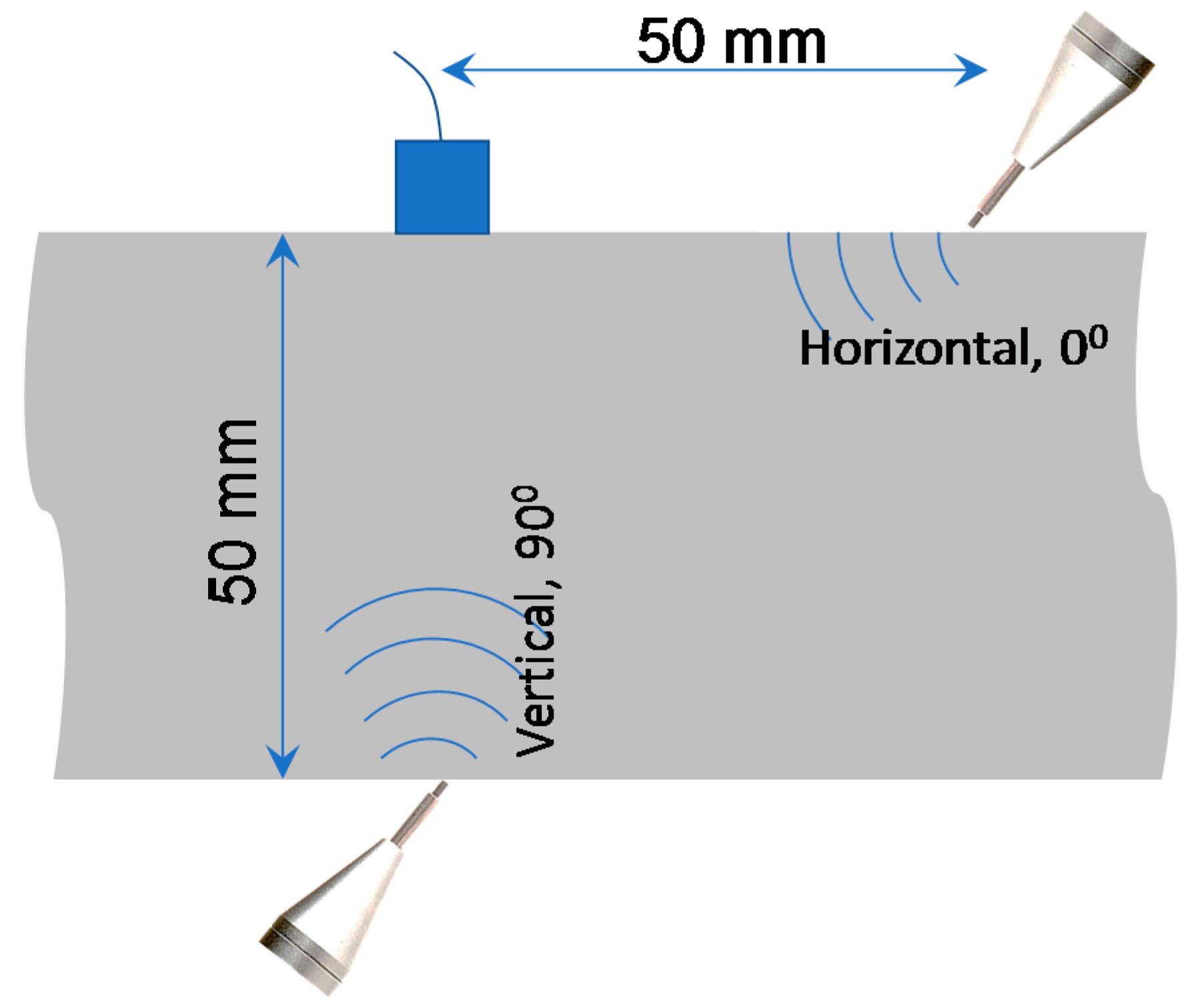
Figure 13.
Individual waveforms received by Pico (5 mm) sensor in the case of (a) horizontal excitation; (b) vertical (c) the average FFT curves of previous waveforms.
Figure 13.
Individual waveforms received by Pico (5 mm) sensor in the case of (a) horizontal excitation; (b) vertical (c) the average FFT curves of previous waveforms.
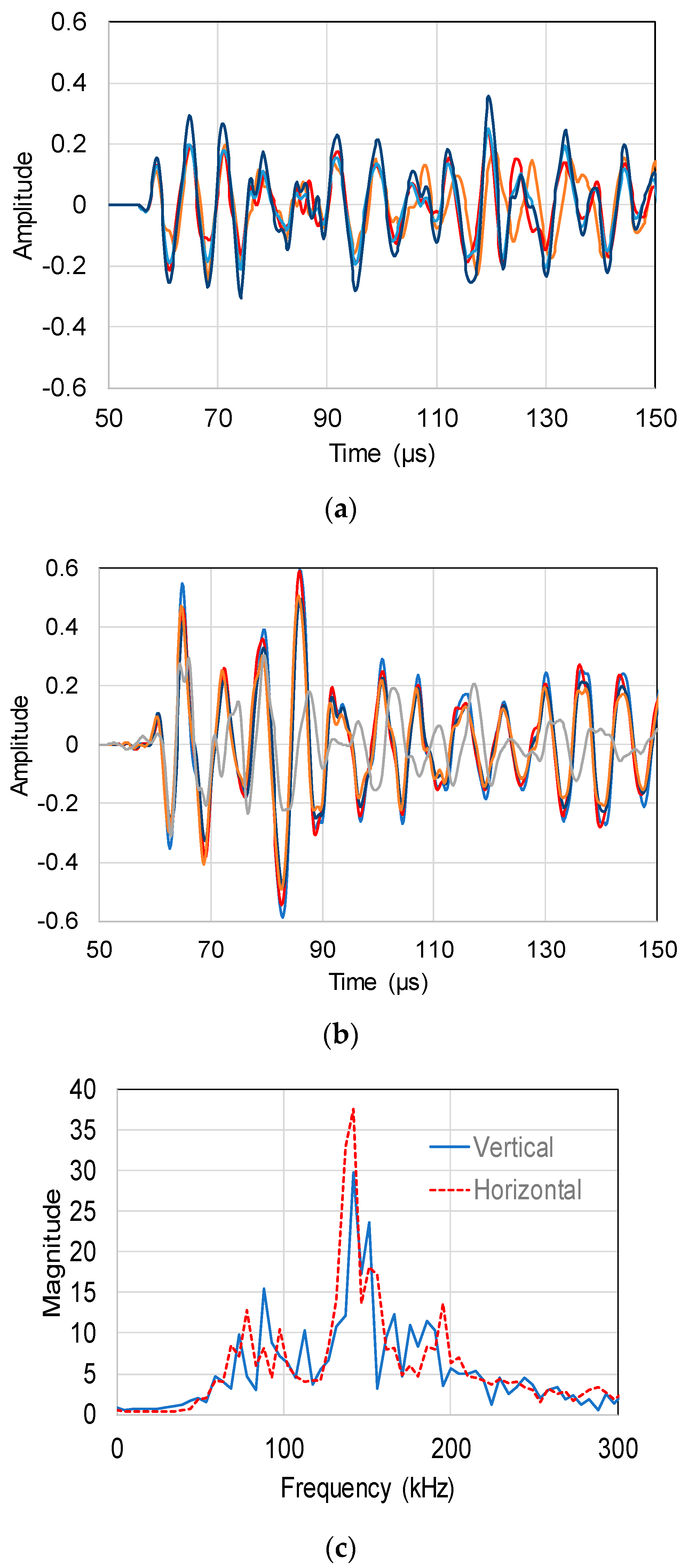
Figure 14.
Waveforms received by long size (R15, 20 mm) sensor in the case of (a) horizontal surface; (b) vertical excitation; (c) The average FFT curves of previous waveforms.
Figure 14.
Waveforms received by long size (R15, 20 mm) sensor in the case of (a) horizontal surface; (b) vertical excitation; (c) The average FFT curves of previous waveforms.
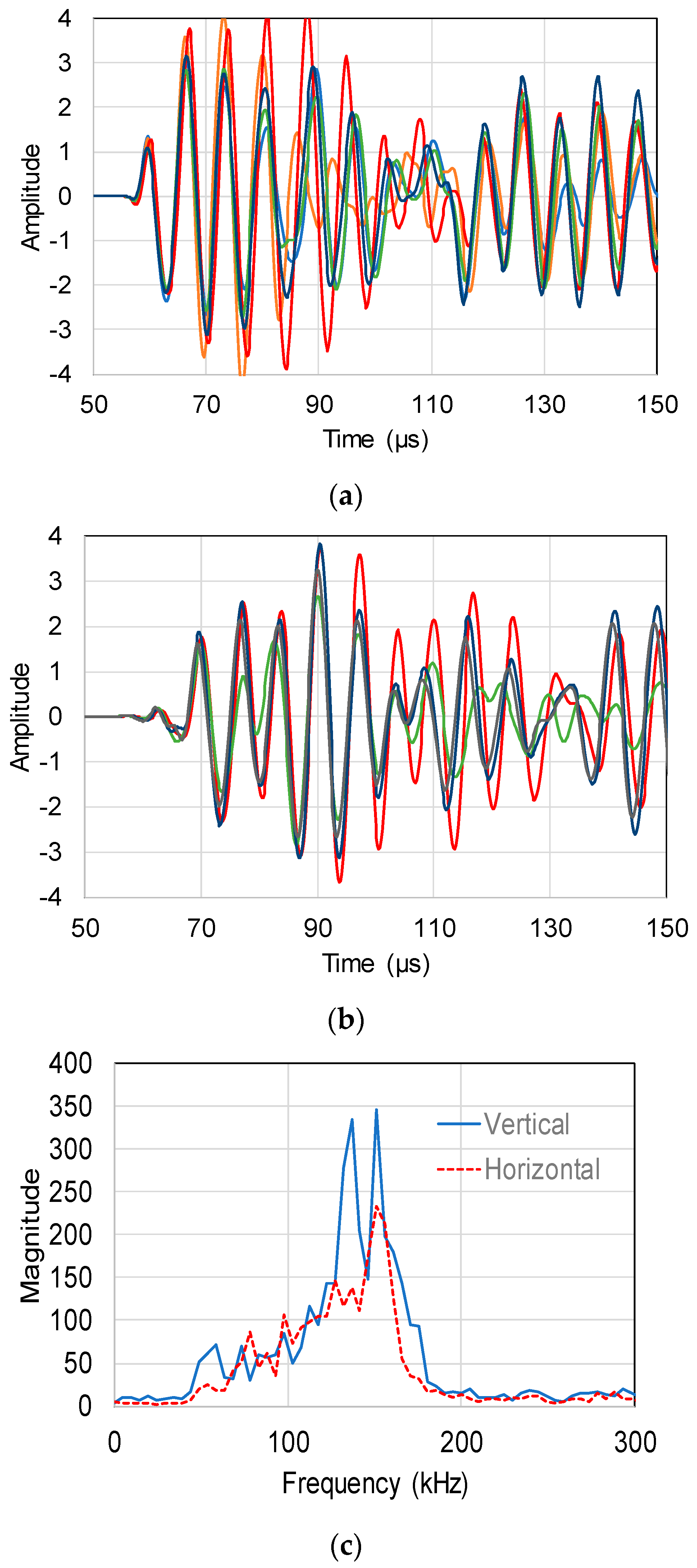
Figure 15.
(a) Simulated waveforms received by 20 mm size sensor after surface source excitation with frequency of 500 kHz and different number of cycles; (b) Relative amplitude vs. waveform length over sensor size.
Figure 15.
(a) Simulated waveforms received by 20 mm size sensor after surface source excitation with frequency of 500 kHz and different number of cycles; (b) Relative amplitude vs. waveform length over sensor size.
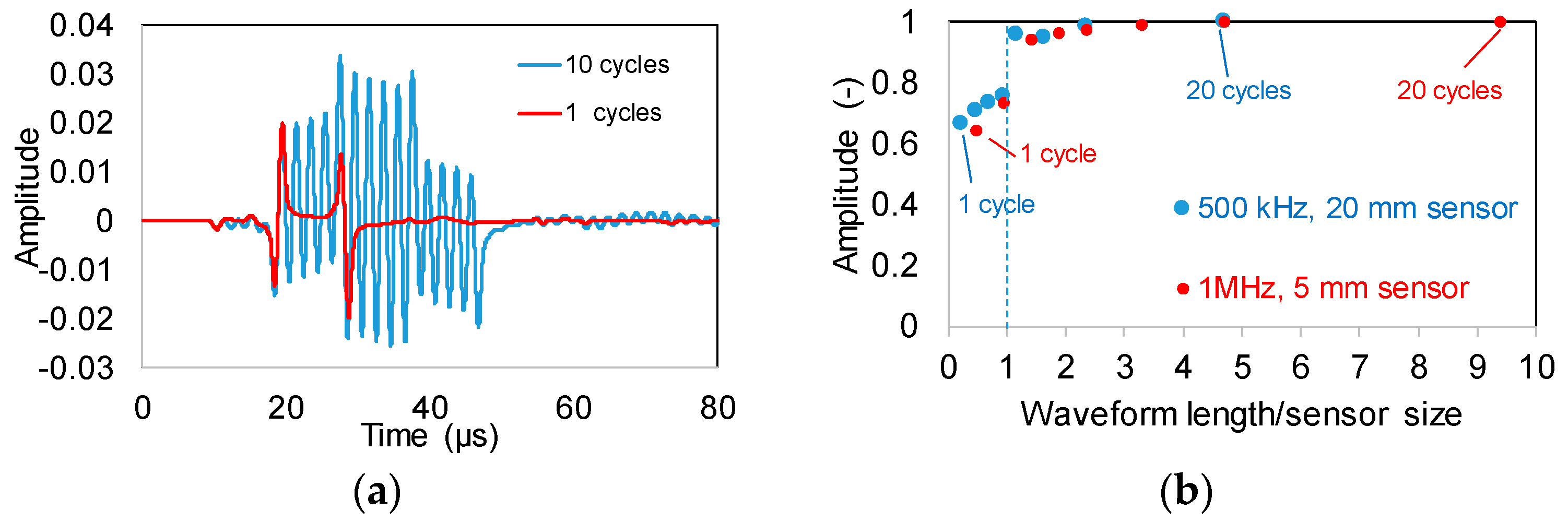
Figure 16.
Simulated waveforms received by different size sensors from surface source with excitation frequency equal to 500 kHz (curves overlap).
Figure 16.
Simulated waveforms received by different size sensors from surface source with excitation frequency equal to 500 kHz (curves overlap).
© 2018 by the authors. Licensee MDPI, Basel, Switzerland. This article is an open access article distributed under the terms and conditions of the Creative Commons Attribution (CC BY) license (http://creativecommons.org/licenses/by/4.0/).
Share and Cite
MDPI and ACS Style
Tsangouri, E.; Aggelis, D.G. The Influence of Sensor Size on Acoustic Emission Waveforms—A Numerical Study. Appl. Sci. 2018, 8, 168. https://doi.org/10.3390/app8020168
AMA Style
Tsangouri E, Aggelis DG. The Influence of Sensor Size on Acoustic Emission Waveforms—A Numerical Study. Applied Sciences. 2018; 8(2):168. https://doi.org/10.3390/app8020168
Chicago/Turabian StyleTsangouri, Eleni, and Dimitrios G. Aggelis. 2018. "The Influence of Sensor Size on Acoustic Emission Waveforms—A Numerical Study" Applied Sciences 8, no. 2: 168. https://doi.org/10.3390/app8020168
Note that from the first issue of 2016, this journal uses article numbers instead of page numbers. See further details here.