A New Resource Allocation Protocol for the Backhaul of Underwater Cellular Wireless Networks


1
Ocean Equipment Research Department Korea Research Institute of Ships & Ocean Engineering (KRISO), Daejeon 34103, Korea
2
Department of Mobile Systems Engineering, Dankook University, Yongin 16890, Korea
*
Author to whom correspondence should be addressed.
Appl. Sci. 2018, 8(2), 178; https://doi.org/10.3390/app8020178
Submission received: 27 December 2017
/
Revised: 20 January 2018
/
Accepted: 23 January 2018
/
Published: 25 January 2018
(This article belongs to the Special Issue Underwater Acoustics, Communications and Information Processing)
Abstract
:Featured Application
Underwater Cellular Wireless Systems.
Abstract
In this paper, an underwater base station initiating (UBSI) resource allocation is proposed for underwater cellular wireless networks (UCWNs), which is a new approach to determine the backhaul capacity of underwater base stations (UBSs). This backhaul is a communication link from a UBS to a UBS controller (UBSC). Contrary to conventional resource allocation protocols, a UBS initiates to re-determine its backhaul capacity for itself according to its queue status; it releases a portion of its backhaul capacity in the case of experiencing resource under-utilization, and also requests additional backhaul capacity to the UBSC if packet drops are caused due to queue-overflow. This protocol can be appropriate and efficient to the underwater backhaul link where the transmission rate is quite low and the latency is unneglectable. In order to investigate the applicability of the UBSI resource allocation protocol to the UCWN, its performance is extensively analyzed via system level simulations. In our analysis, considered performance measures include average packet drop rate, average resource utilization, average message overhead, and the reserved capacity of the UBSC. In particular, the simulation results show that our proposed protocol not only utilizes most of the given backhaul capacity (more than 90 percent of resource utilization on the average), but also reduces controlling message overheads induced by resource allocation (less than 2 controlling messages on the average). It is expected that the simulation results and analysis in this paper can be used as operating guidelines to apply our new resource allocation protocol for the UCWN.

1. Introduction
Nowadays, the range of underwater applications is getting wider; those applications include not only underwater surveillance and enemy detection for tactical purpose, but also observation of underwater ecosystem, development of underwater natural resources, underwater plants construction, underwater robot manipulation, and Internet of underwater things (IoUT) for commercial purposes [1,2,3]. In order to manage these applications and to obtain a huge volume of collected data, an underwater communication network is as necessary as a terrestrial communication network [4]. In the view of accessibility, economic feasibility, network expandability, and applicability, it is preferable to build an underwater wireless network to an underwater wired network. Additionally, an acoustic frequency is mainly employed as a communication medium because acoustic signals support longer communication range and experience less signal attenuation than radio-frequency (RF) and optical signals in spite of its limited bandwidth (e.g., tens of kHz) and long propagation delay ( order higher than RF signals) [5,6].
An underwater sensor network is a representative underwater wireless network, where multiple sensor nodes form a cluster. The data from a sensor node in one cluster is transmitted to that in another cluster by exchanging data between cluster heads. An underwater sensor network is advantageous due to its simplicity to build a network infrastructure, application versatility, and network expandability. However, this network type may suffer from severe latency, packet loss, and resource under-utilization induced by the bottleneck (e.g., due to heavily loaded traffic) occurred at a cluster head [7]. Moreover, message overhead can increase due to transferring routing messages among cluster heads and frequent re-routing owing to the mobility of nodes [8].
In order to reliably operate underwater applications and to overcome the weakness of an underwater sensor network, an underwater cellular wireless network (UCWN) was considered in the previous studies [8,9]. In a UCWN, an underwater base station (UBS) located at the center of a cell controls underwater terminals (UTs) residing in its cell, which is very similar to a terrestrial cellular wireless network (TCWN) [10]. In one underwater cell, a UBS collects data from all the UTs, and forwards the data to a UBS controller (UBSC) which is located on the water surface and controls multiple underwater base station (UBSs). A UBSC can be fixed (like a buoy) or mobile (like a command ship) dependent upon applications. The communication link between a UBS and a UBSC is important because it is responsible for exchanging both control signaling and data traffic. This link is very similar to the backhaul link between a base station and a base station controller in a TCWN. Thus, it can also be regarded as a backhaul link between a UBS and a UBSC. A UCWN can improve performance in terms of latency by avoiding multi-hop communications, thus enhancing network efficiency [11]. Furthermore, a UCWN may increase the communication reliability in harsh underwater environments where frequent transmission failure due to high bit error rate (BER) occurs and network traffic is heavily loaded caused by the advance of underwater applications [11,12].
Previously, several studies for a UCWN have been done since the introduction of the concept of a UCWN in literature [8,9,10]. The studies to design the topology of a UCWN was done in [11,13,14]; a cell radius, spatial frequency reuse pattern, the available number of UTs per cell, and the capacity per cell are mathematically derived by considering the given bandwidth and signal-to-interference ratio (SIR). A few guidelines targeted for planning a UCWN are also suggested via extensive simulation works. In [15], a collision-free medium access control (MAC) protocol was proposed for a UCWN to completely avoid collisions among UTs located in a cell; a UBS sets UTs’ tier according to their distance from the UBS, and manages UTs’ transmission scheduling corresponding to the tier.
In addition, a resource allocation protocol, which determines the backhaul capacity of UBSs being applied to its backhaul link, was primarily proposed for a UCWN in [16] by considering following remarkable differences between the backhaul link of a UCWN and that of a TCWN.
- Traffic volume. The amount of the uplink traffic (i.e., from a base station to a base station controller) is much larger than that of the downlink traffic (i.e., from a base station controller to a base station) in a UCWN, which is completely contrary to a TCWN.
- Performance. The transmission rate of a backhaul link of a UCWN is much lower than that of a TCWN. Besides, the latency of a backhaul link of a UCWN is much higher than that of a TCWN.
The differences mentioned above and asymmetrically increasing traffic of UBSs due to applying various underwater applications result in the traffic congestion in backhaul links of a UCWN. The protocol in [16] helps a UCWN deal with this bottleneck occurred at the backhaul link; a UBSC adaptively allocates the backhaul capacity of a UBS being proportional to its input traffic (i.e., the data collected from UTs in its cell), and thus improves backhaul transmission efficiency and fairness. To do this, a UBSC allocates several time slots per frame to UBSs for their backhaul capacity based on time division multiple access (TDMA). Three input traffic values are considered: current traffic, accumulated mean traffic, and the maximum traffic. Also, two methods that a UBS sends its input traffic to a UBSC are employed according to whether the transmission period is fixed or not: fixed period and adaptive period. It was shown via simulations that sending accumulated mean traffic with adaptive period mostly guarantees the best performance [16].
In spite of its novelty, the resource allocation technique described in [16] still needs to be enhanced considering the following aspects.
- The ability to manage drastic change of uplink traffic. As the protocol in [16] was designed under the assumption that the UBSC capacity is enough to manage the input traffic from all the UBSs, it can be partially efficient when the uplink traffic of all the UBSs does not change quickly or does not show any bursty nature (which can be caused by mobile UTs such as autonomous underwater vehicles (AUVs)). However, in practice, it is possible that the uplink traffic of a UBS may abruptly increase due to burst traffic caused by mobile UTs or the rise of traffic gathered from (fixed) UTs in its cell. This can make a UBSC experience a shortage of backhaul capacity, and consequently it suffers from long latency and packet drops by queue-overflow. Thus, a more responsive resource reallocation reflecting traffic condition, that the uplink traffic of each UBS changes fast or the outbreak of burst uplink traffic occurs frequently, is strongly required.
- The way to readjust the backhaul capacity of a UBS. In [16], a UBSC collects traffic information from all the UBSs, calculates their backhaul capacity, and periodically reassigns their backhaul capacity by informing them of their new backhaul capacity. In other words, all the UBSs must communicate with a UBSC for the readjustment of their backhaul capacity at the same time. This is quite inefficient to the backhaul link of a UCWN suffering from both low transmission rate and high latency because the message overhead for reallocation of the backhaul capacity is quite large. Thus, considering low transmission rate and high latency of the backhaul links, a more efficient method to reassign the backhaul capacity of UBSs is necessary.
- Interoperability. As there are diverse modulation and coding schemes (MCSs) and multiple access schemes such as FDMA (Frequency Division Multiple Access), TDMA, CDMA (Code Division Multiple Access), and OFDMA (Orthogonal Frequency Division Multiple Access) for different underwater communication links and ranges, a resource allocation protocol, which is interoperable with diverse MCSs and multiple access schemes, is required.
Hence, it is necessary to design a new resource allocation protocol for the backhaul of a UCWN which considers more realistic underwater communication environments.
In this paper, we propose a novel resource allocation protocol for a UCWN by considering the characteristics of an underwater backhaul link as stated above. It effectively determines the backhaul capacity of UBSs responding to both fast uplink traffic change and burst traffic cases with a much smaller amount of message overhead, which is required for the reallocation of the backhaul capacity. In our approach, all of the capacity of the UBSC is not assigned to all the UBSs at once, being proportional to their uplink traffic. Instead, the UBSC determines the backhaul capacity of all the UBSs considering the upper limit (or the pre-determined maximum capacity) as well as uplink traffic of each UBS. More specifically, the UBSC calculates the backhaul capacity of each UBS proportional to the amount of input traffic of the UBS. If the calculated backhaul capacity of a UBS is greater than pre-determined upper limit, then the backhaul capacity of the UBS is determined as the upper limit. Otherwise, the backhaul capacity of the UBS is determined as the calculated value. So, some portion of the total backhaul capacity will not be allocated to the UBSs, and it is reserved at the UBSC. This reserved backhaul capacity is used to provide additional backhaul capacity to the UBS which requests more backhaul capacity due to abrupt traffic increase from UTs or burst traffic from mobile UTs (such as AUVs). In general, a UBS requesting more backhaul capacity may have already experienced packet drops due to queue-overflow. On the other hand, when a UBS uses lower backhaul resource than its allocated backhaul capacity, it returns some portion of its capacity to the UBSC, which will be added to the reserved backhaul capacity of the UBSC. And the reserved capacity can be used to support any UBS requesting additional backhaul capacity later.
In the conventional resource allocation scheme in [16], the UBSC always initiates the backhaul resource allocation and determines the backhaul capacity of each UBS. In this scheme, the UBSC must communicate with all the UBSs to collect information for the reallocation. On the contrary, in our scheme, a UBS can initiate backhaul resource reallocation. Therefore, we call it “UBSI (UBS Initiating)” resource allocation protocol. Moreover, the UBSC communicates with only one UBS for resource reallocation if the reserved backhaul capacity in the UBSC is larger than the requested backhaul capacity of the UBS. In other words, our approach has much less resource reallocations, wherein the UBSC communicates with all the UBSs, than the conventional approach. Thus, our approach is expected to reduce the message overhead for the resource reallocation, and can be efficient for underwater communication links with low data rate and high latency.
Besides, in terms of interoperability, our UBSI resource allocation protocol determines the backhaul capacity of a UBS as a ratio to total backhaul capacity, which is interoperable with any multiple access technique.
In order to analyze the performance of our new resource allocation protocol, we perform system level simulations (SLSs) under the environments consisting of one UBSC and multiple UBSs. We consider four performance measures: average packet drop rate, average resource utilization, average message overhead, and reserved backhaul capacity in the UBSC. In our SLSs, these four performance measures are investigated with respect to the average input traffic and the average burst traffic of UBSs by considering two scenarios:
- Scenario 1: varying the upper limit (or maximum) of the backhaul capacity of a UBS,
- Scenario 2: varying the lower limit of the resource utilization threshold where a UBS returns unused backhaul capacity when its current resource-utilization becomes less than this lower limit.
For each scenario, we provide a summary of our SLS results and analysis, and an operational guideline for the backhaul resource allocation in the UCWN using the proposed UBSI protocol.
The remaining part of this paper is organized as follows. In Section 2, the structure of a considered UCWN is described. In Section 3, a new resource allocation protocol is specified in detail, including its queue model, the way to determine the backhaul capacity of a UBS, and the corresponding protocol messages and procedures. In Section 4, the performance is investigated via extensive system level simulations considering two scenarios. Finally, in Section 5, we conclude this paper.
2. System Description
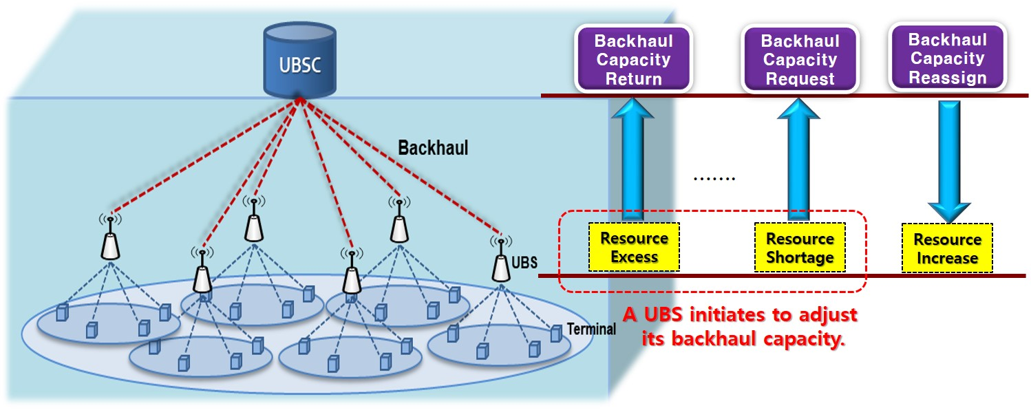
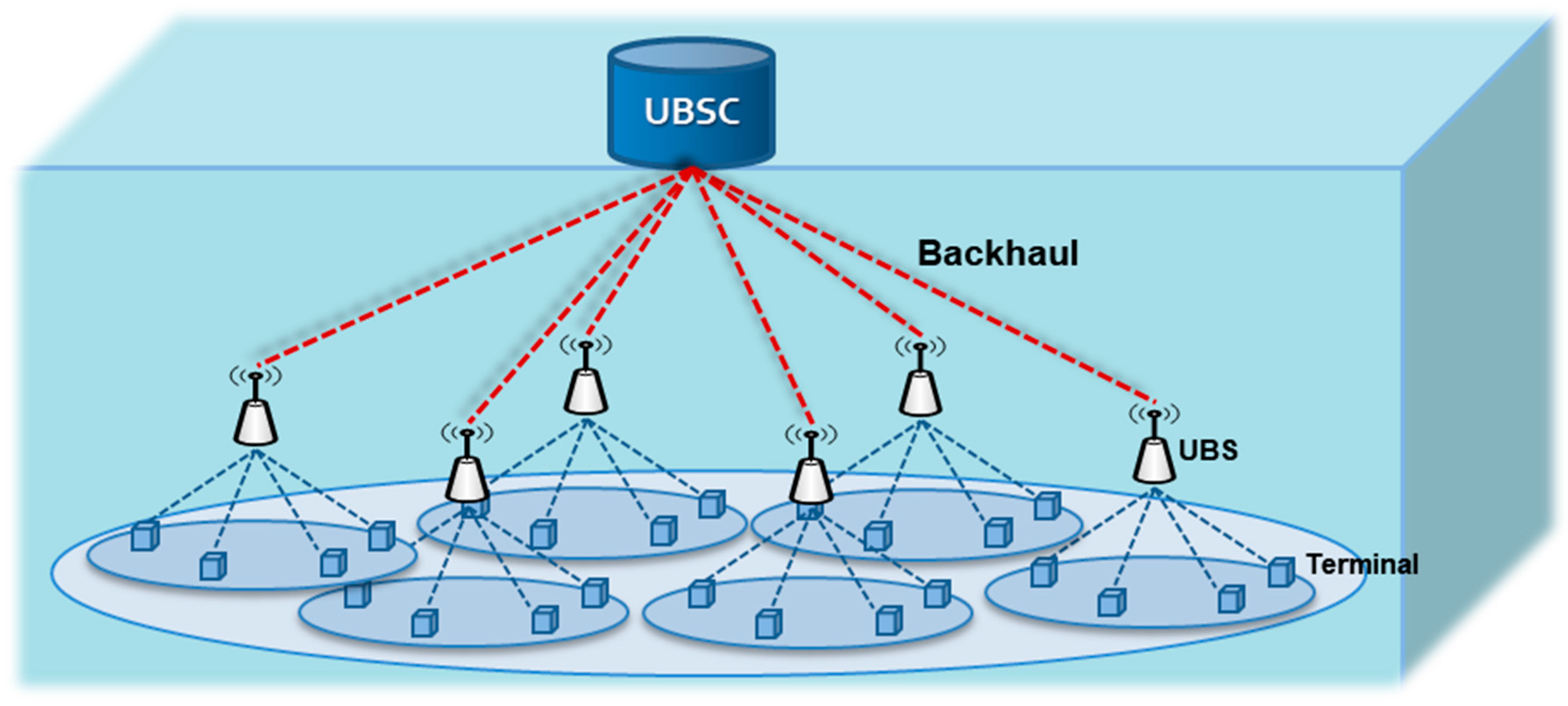
We consider a UCWN as shown in Figure 1, where there is one UBSC and multiple UBSs. Each UBS communicates with many UTs (or underwater nodes) in its cell. UTs collect surrounding information and transmit the information to the UBS. We also consider a special type of UT such as AUV which moves from one cell to another. This is connected with a UBS, and transmits much larger volume of traffic than normal UTs. In other words, we consider two types of UTs: the first type is just normal fixed UTs like sensors, which transmit a small amount of data in periodic manner, the second type is a mobile UT like an AUV, which transmits a much larger amount of data. We assume that there are a large number of first type UTs and a few second type UTs.
In a UCWN, a UBSC is connected with many UBSs through underwater wireless backhaul as illustrated in Figure 1. There are two communication links: one is the link from the UBSC to the UBS (called downlink), and the other is from the UBS to the UBSC (called uplink). We can assume that uplink has much more traffic than downlink and thus requires much larger backhaul capacity than downlink. This is a reasonable assumption because a UBSC mostly transmits control signaling to UBSs. However, a UBS collects data from many UTs and transmits the data to the UBSC. This motivates us to design an efficient resource allocation protocol for the uplink backhaul in this UCWN throughput this paper.
3. Description of UBSI Resource Allocation Protocol
In this section, a new resource allocation protocol for a UCWN called UBS Initiating (UBSI) resource allocation protocol is described, including its queue model, the way to determine the backhaul capacity of a UBS, and the corresponding protocol messages and procedures. While it is common to [16] and the UBSI resource allocation protocol that the backhaul capacity of a UBS is determined to be proportional to its uplink traffic, the followings are remarkable differences between them.
- The UBSI resource allocation protocol is basically designed to efficiently manage the non-guaranteed UBSC capacity which implies that the capacity of the UBSC is insufficient to deal with the uplink traffic induced by UBSs.
- A UBS triggers to adjust its backhaul capacity for itself according to its queue status which does not affect the actions of other UBSs. To do this, a UBS requests additional backhaul capacity in case of occurring packet drops due to the shortage of current backhaul capacity. This can improve the performances of a UCWN in terms of energy efficiency, message overhead, throughput, and latency. A UBS also returns a portion of its backhaul capacity to the UBSC when it detects that its resource is under-utilized in order to manage the limited backhaul capacity of the UBSC.
- A ratio-based backhaul capacity is employed in order to be interoperable with any multiple access protocols (e.g., TDMA, CDMA, FDMA, or OFDMA) which have different resources, respectively.
3.1. Queue Model and Backhaul Capacity of UBSs
3.1.1. Queue Model
A UBS can be modelled as a queuing system as illustrated in Figure 2, where the arrival rate and the service rate represent the input traffic from UTs located in its cell and the backhaul capacity of the UBS allocated by the UBSC, respectively. This queue model helps a UBSC to allocate the total backhaul capacity to all the UBSs. Basically, the backhaul capacity of each UBS will be proportional to its input traffic. However, note that there is the maximum backhaul capacity of a UBS in the proposed UBSI resource allocation protocol.
In the following, we explain several parameters in Figure 2.
- is the arrival rate of a UBS during the -th time interval. In other words, this is the number of packets of a UBS received from all the UTs residing in its cell during the -th time interval.
- is the service rate a UBS during the -th time interval. That is, this implies the number of packets served by UBS during the -th time interval. Once the backhaul capacity of a UBS is determined, it holds until the next reallocation. And a UBS transmits its uplink traffic with the data rate up to its backhaul capacity. is the queue length of a UBS at the end of the -th time interval. Specifically, this is the number of packets remaining at the queue of UBS at the end of the -th time interval. The queue length of a UBS is expressed as a function of its previous queue length at time interval − 1, the current input traffic (i.e., packet arrival) rate and the backhaul capacity during time interval . Besides, the queue length has its maximum value denoted by . Thus, it is expressed as the following equation.
- is the number of packet drops of a UBS during the -th time interval. In other words, this is the number of packets dropped from the queue of a UBS during the -th time interval. Similar to the is a function of its previous queue length at time − 1, the current input traffic (i.e., packet arrival) rate and backhaul capacity during time interval , and represented as
The parameters used in the UBSI protocol are summarized in Table 1.
3.1.2. Backhaul Capacity of UBSs
The backhaul capacity of a UBS is determined by the corresponding UBSC. The UBSC calculates the backhaul capacity of the UBS by considering the traffic information sent from the UBS. The traffic information includes the queue length and the number of packet drops of the UBS. Each traffic information is a mean value averaged during a period which is a positive integer and its value can be changed as a network parameter. The mean value of the queue length is represented as
The average number of packet drops of a UBS, denoted by , can be obtained similar to the Equation (3).
Using the sum of averaged queue length and packet drops (i.e., and ), the backhaul capacity of a UBS is proportionally determined on the basis of a linear-proportional algorithm as in [17,18,19]. And the backhaul capacity, denoted by , is also limited no more than the predetermined maximum value , and thus expressed as
The backhaul capacity of a UBS will actually be determined by considering the multiple access protocol used in the real UCWN. For example, in case of TDMA, the backhaul resource of a UBS is given by the number of slots per TDMA frame, being proportional to its calculated backhaul capacity. In case of FDMA, the backhaul resource of a UBS is the channel bandwidth, or the number of narrow band channels.
Using Equation (4), the reserved capacity of a UBSC at the time , which can be utilized to readjust the capacity of all UBSs on occasion, is also expressed as
3.2. Protocol Messages and Procedures
The UBSI resource allocation protocol consists of two phases: the initialization phase (denoted by “IP”) and the normal operation phases (denoted by “NP”). In the view of resource allocation, the backhaul capacity of all UBSs are initially determined with respect to their initial traffic information in the initialization phase, while that of all UBSs is reallocated according to their current queue status.
3.2.1. Protocol Messages
All messages of the UBSI resource allocation protocol is equivalently applied as in [16]:
- A Resource Information Request (RIREQ) is a message that a UBSC asks all UBSs to send their traffic information as specified in Section 3.1.1.
- A Resource Information Response (RIREP) is a response message to RIREQ sent by a UBS which includes its traffic information.
- A Resource Allocation Information Send (RAIS) is a message sent by a UBSC to inform a UBS sending a RIREQ of new backhaul capacity. During the IP, this message contains allocated backhaul capacity of each UBS and is broadcasted to all the UBSs. However, during the NP, this message contains reallocated backhaul capacity of a UBS which requested reallocation of its backhaul capacity. Thus, in this case, this message is sent to only one UBS.
- A Resource Allocation Information Send Acknowledgement (RAISACK) sent by a UBS is an acknowledgement message of RAIS.
- A Resource Reallocation Request (RAREQ) is a message that a UBS asks a UBSC to adjust its backhaul capacity.
- A Resource Reallocation Acknowledgement (RAACK) sent by a UBSC is an acknowledgement message of the RAREQ.
Table 2 shows the summary of the messages used in the UBSI protocol. For each message, the tables shows the direction of message, the phase when the message is used, and the transmission type.
3.2.2. Initialization Phase
The initialization phase is executed in two cases. One is at the beginning of a UCWN. The other is when a UBSC lacks its reserved capacity to provide a UBS with additional backhaul capacity in the normal operation phase, and thus decides to return to the initialization phase. At the beginning of a UCWN, the initial resource to send any message of a UBS is assumed to be provided using a given MAC protocol.
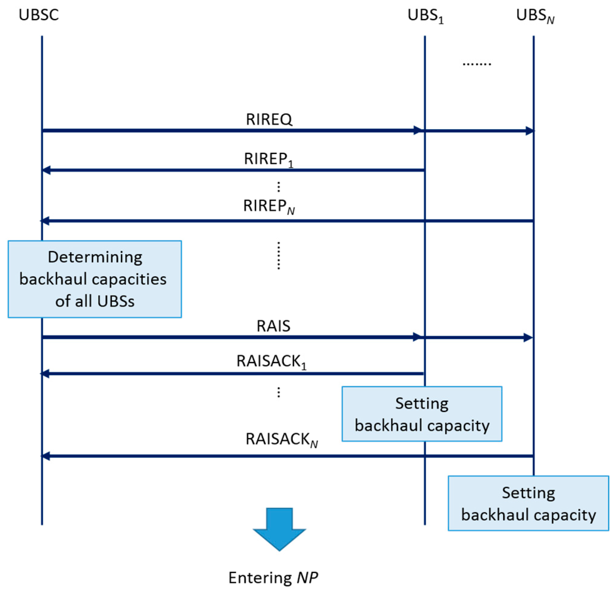
A UBSC starts this phase by broadcasting an RIREQ message as shown in Figure 3. Any UBS which receives the RIREQ message sends an RIREP message to the UBSC which includes its traffic information (i.e., and ). If the UBSC receives RIREPs from all UBSs, it determines their backhaul capacities as explained in Section 3.1.2. Then, the UBSC broadcasts an RAIS message which includes the backhaul capacity information of all UBSs and waits for their responses, i.e., RAISACK messages. After receiving the RAIS message, a UBS enters the normal operation phase by sending its uplink traffic to the UBSC.
A UBSC maintains a traffic information table, which includes traffic information of all the UBSs, to utilize it as a reference to calculate their backhaul capacities in the two phases. In addition, a UBS also keeps track of the number of packet drops and the resource utilization values in order to ask the UBSC to adjust its backhaul capacity. The resource utilization of a UBS at time , denoted by , is the degree of using given backhaul capacity. This quantity is defined as a ratio of the served number of packets to the given backhaul capacity, and its maximum value is one. Thus, it is expressed as
3.2.3. Normal Operation Phase
In the normal operation phase, a UBS sends as much uplink traffic to a UBSC as its backhaul capacity. And it also consistently updates its queue status including the queue length, the packet drop rate, and the resource utilization. A UBS requests an adjustment of its backhaul capacity to a UBSC for two cases: (1) resource under-utilization and (2) queue-overflow due to the lack of backhaul capacity.
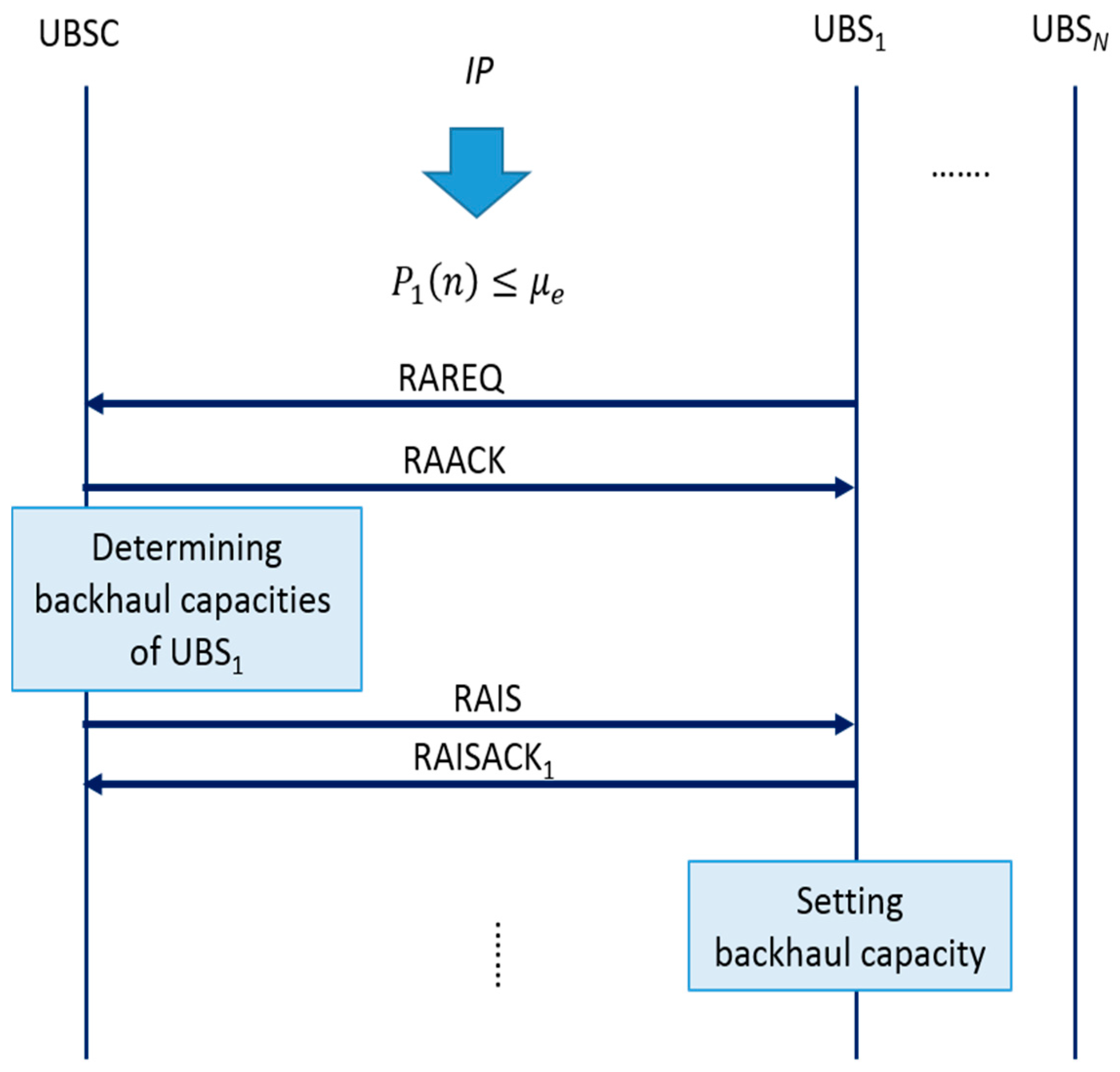
In the case of resource under-utilization (determined by the condition: ) where is the lower limit of resource utilization as a network parameter, a UBS returns a portion of its backhaul capacity to the UBSC. The effects of on the performance are summarized as follows.
- As decreases, the frequency of backhaul capacity adjustment decreases since a UBS will have less probability of the event . Thus, it is expected to improve energy efficiency and to have less message overhead, but to deteriorate overall resource utilization, throughput, and packet drop rate.
- As increases, the frequency of backhaul capacity adjustment increases since a UBS will have higher probability of the event . The performance pattern is expected to be opposite to when decreases. This implies that a performance trade-off exists between these two situations.
To manage resource under-utilization, a UBS sends an RAREQ message to the UBSC, as illustrated in Figure 4. When the UBSC receives the RAREQ message, it sends an RAACK message to the UBS. Then, the UBSC updates a traffic information table by including new traffic information of the UBS and calculates the backhaul capacity of the UBS as specified in Section 3.1.2. The return of backhaul capacity implies the rise of the reserved capacity of the UBSC, denoted by , this can be used to help another UBS suffering from the shortage of backhaul capacity. The UBSC sends a RAIS message to the UBS and waits for a RAISACK message as shown in Figure 4.
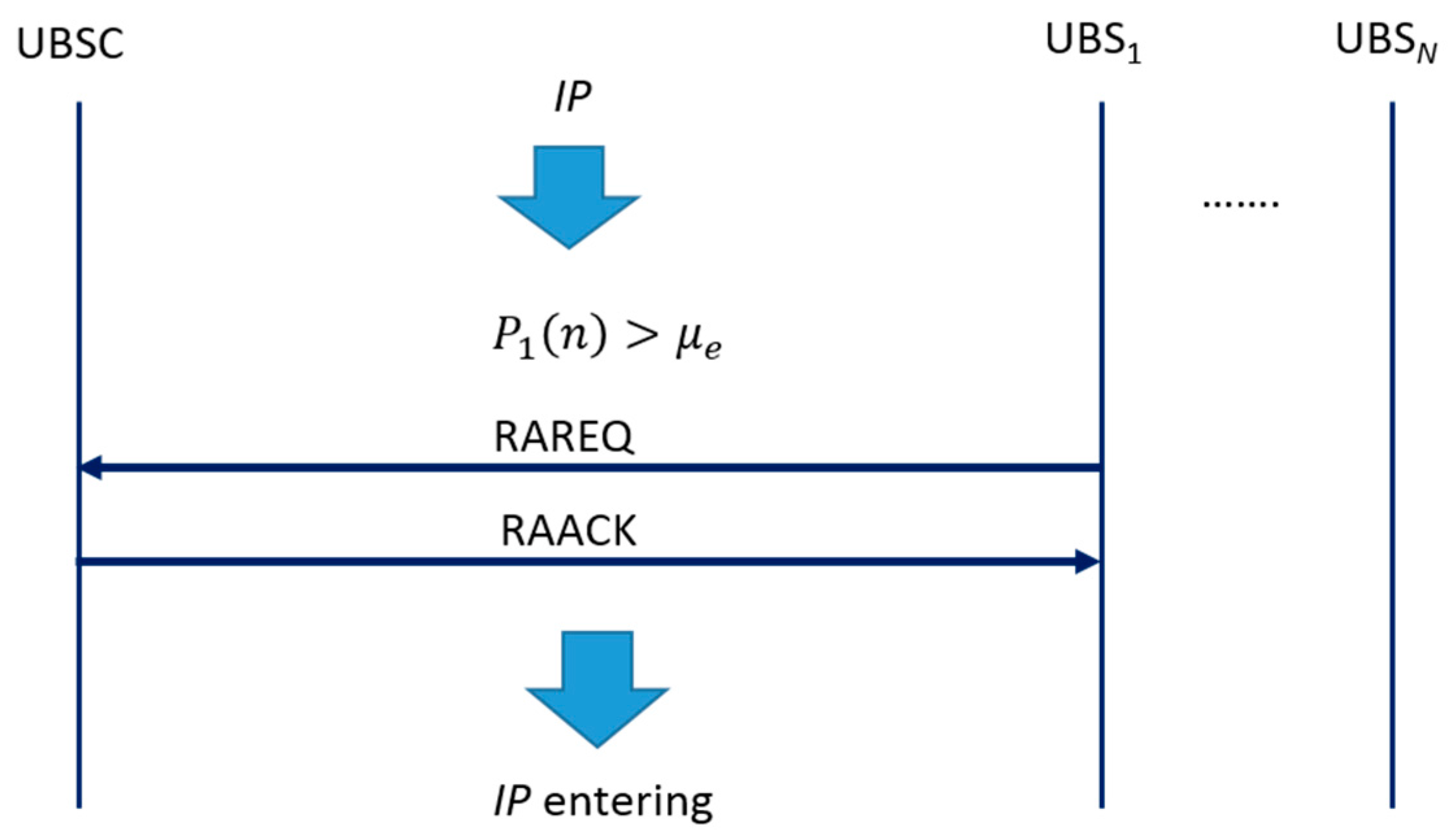
In the case of queue-overflow (determined by the condition: a UBS experiences the packet drop of input traffic due to the lack of backhaul capacity. In this case, the UBS sends an RAREQ message to the UBSC in order to request additional backhaul capacity, as illustrated in Figure 5.
When the UBSC receives the RAREQ message, it sends an RAACK message to the UBS and calculates new backhaul capacity of the UBS as specified in Section 3.1.2. The UBSC also determines the required backhaul capacity and compares it to the reserved capacity of the UBSC, i.e., . Here, the required backhaul capacity is expressed as where and are newly determined backhaul capacity and current backhaul capacity of the UBS, respectively. If the reserved capacity of the UBSC is greater than the required backhaul capacity, that is , the UBSC sends an RAIS message and remaining procedures are executed as shown in Figure 5. If the reserved capacity of the UBSC is insufficient to provide the required backhaul capacity, i.e., , the UBSC broadcasts an RIREQ message to all the UBSs and goes back to the initialization phase, as shown in Figure 6. The remaining procedures are the same as those in Section 3.2.2.
4. Simulation and Performance Analysis Results
In order to examine the performance of the UBSI resource allocation protocol for a UCWN, we performed system level simulations (SLSs). This SLS includes all the details of the UBSI resource allocation protocol described in Section 3. In this section, we describe the SLSs in detail and the simulation results for the different simulation parameters.
4.1. System Level Simulation Description and Performance Measures
In the SLSs, we considered an uplink backhaul link of a UCWN, where there are one UBSC, ten UBSs with multiple UTs, and a few mobile UTs like AUVs. We assumed that each UBS receives the packet from the UTs connected to the UBS with Poisson distribution with the packet arrival rate . In other words, each UBS receives different amounts of packets with Poisson distribution, but all the UBS have the same average packet arrival rate . In addition, we assumed that there are a few mobile UTs in the UCWN, which communicate with one of the UBSs in the UCWN, and there is only one mobile node in the UBS. So, the UBS communicating with a mobile UT will receive burst traffic from the mobile UT with Poisson distribution with much higher arrival rate .
The parameters used in the SLSs are listed in the Table 2. We performed simulations for different sets of the parameters. For each simulation, some parameters are used as default values and others are changed to investigate the different perspectives of the performance. We also considered four performance measures in the SLSs which are mean values of all UBSs and defined as follows.
- Average packet drop rate: a ratio of dropped packets over ingress packets in a queues of a UBS.
- Average resource utilization: a ratio of used backhaul capacity over assigned backhaul capacity of a UBS.
- Average message overhead: the number of messages induced by resource reallocation.
- Average reserved UBSC capacity of the UBSC.
4.2. Simulation Results and Performance Analysis
In this paper, we performed many different SLSs for different parameter sets, but we show only some remarkable results in this section. As stated in Section 1, we considered two simulation scenarios as follows:
- Scenario 1: varying the upper limit (or maximum) of the backhaul capacity of a UBS.
- Scenario 2: varying the lower limit of the resource utilization threshold where a UBS returns unused backhaul capacity when its current resource-utilization becomes less than this lower limit.
4.2.1. Scenario 1
Here, we investigated the four performance measures for different under-utilization limit ( and the number of mobile UTs (. To do this, we changed the value of from 0.3 to 0.7, and that of from 1 to 2. The burst traffic, generated from each mobile UT, arrives at the UBS with Poisson arrival rate 30 (i.e., the mean inter-arrival time is given as ). And the average packet arrival rate of each UBS, denoted by , is changed from 3 to 20.
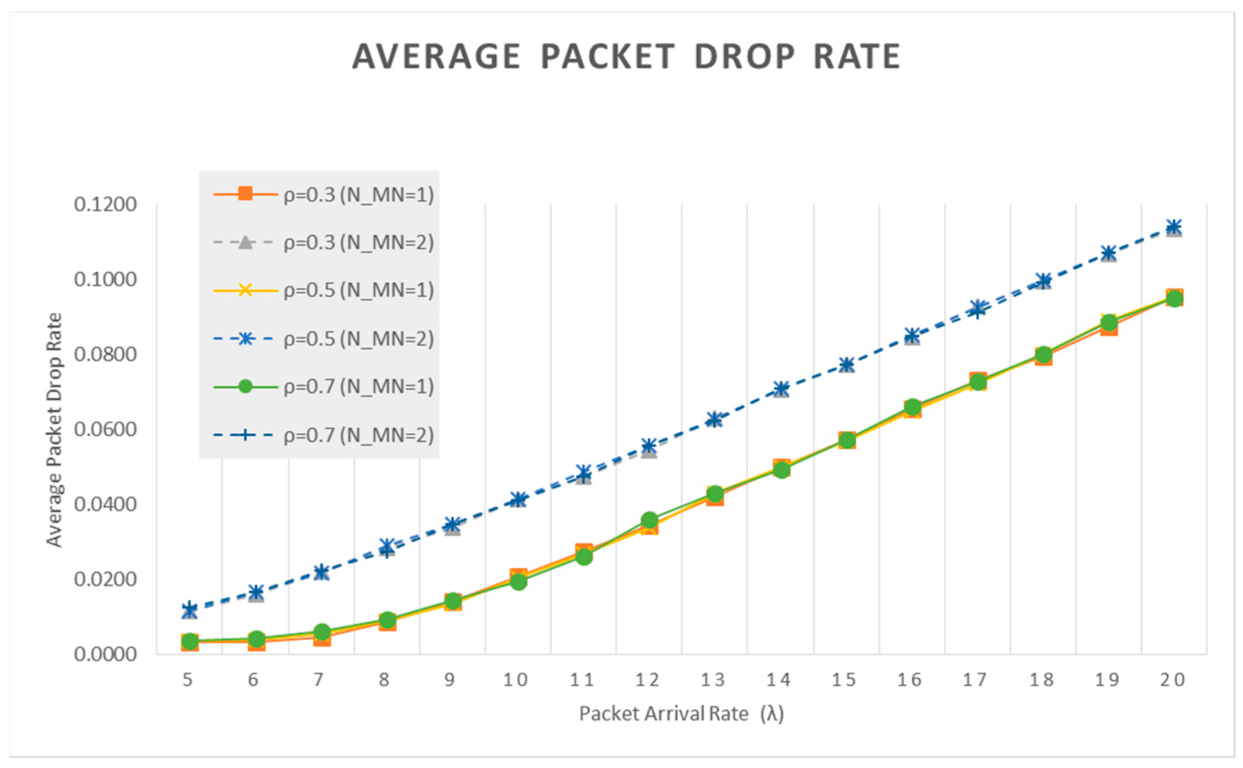
Figure 7 shows the average packet drop rate for this case. (In the following four graphs, is simply denoted by for convenience sake.) As shown in Figure 7, the average packet drop rate increases as the average packet arrival rate increases. In the graph, we can find that the average packet drop rate is notably different dependent upon the number of mobile UTs ; the average packet drop rate performance becomes worse as the value of increases. However, the average packet drop rate is almost the same for different values of under-utilization limit
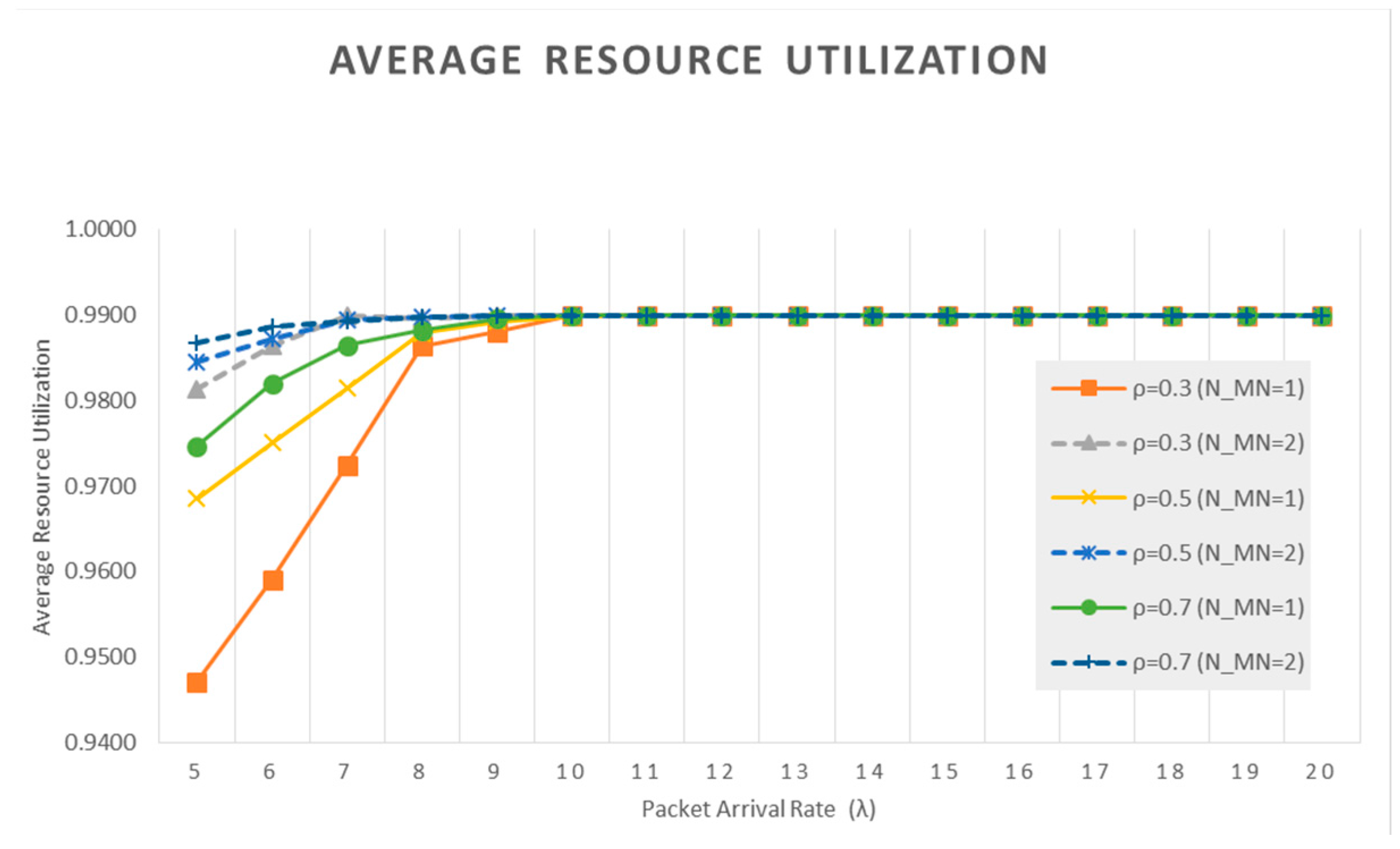
Figure 8 shows the average resource utilization for this case. As shown in the figure, the average resource utilization approaches to almost 99% as the packet arrival rate increases. We can find the different resource utilization values when is small (i.e., ). In addition, when is small such as from 5 to 7, average resource utilization for the case = 1 is much lower than the case = 2. This is obvious since there are more packet arrival in the case = 2, and the burst traffic is a more dominant factor when is small. When = 1 and = 5, the average resource utilization becomes higher as increases. The reason is as follows. As increases the UBS returns the backhaul resource more frequently to the UBSC if its resource is under-utilized. So, the average resource utilization becomes higher, and the message overhead due to the return procedure increases. This phenomenon can be observed in Figure 9.
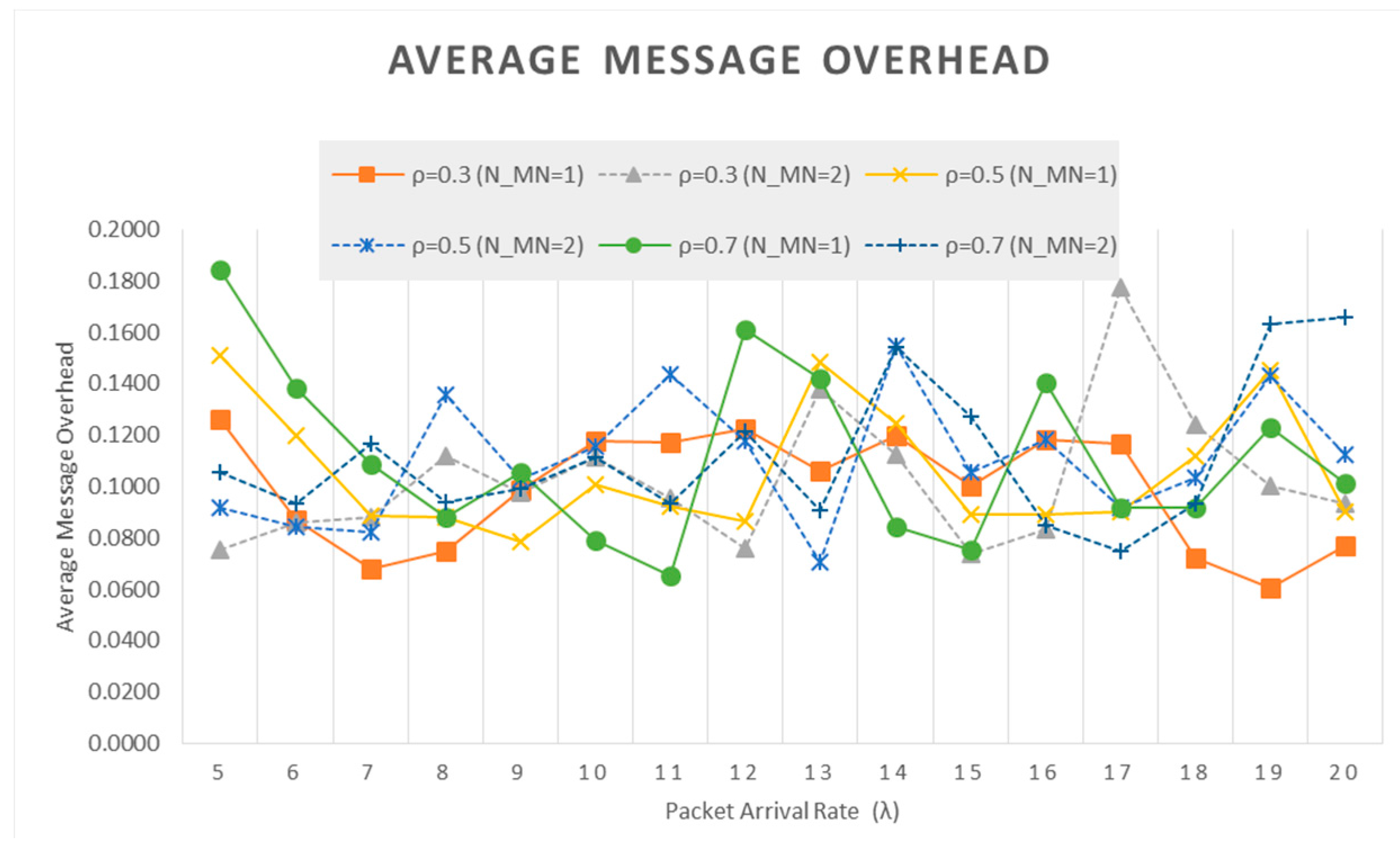
Figure 9 shows the average message overhead for this case. It is shown that the message overhead of the UBSI resource allocation protocol is remarkably small because control signaling message mostly occurs when the UBSC reallocate backhaul resources for the UBSs according to their requests. As described in Section 3, this reallocation is caused by the two cases. The first case is when the resource of a UBS is under-utilized, and the second case is when a UBS has packet drop due to the shortage of the backhaul capacity. When the average packet arrival rate is small, message overhead is mainly caused by under-utilization. Thus, we can observe that situation as illustrated in Figure 9. In the figure, when is small (e.g., ), average message overhead becomes larger as becomes higher and smaller.
As becomes larger, the average message overhead fluctuates. This fluctuation occurs because the resource reallocation in the UBSC is mainly triggered by packet drops in the UBSs. And this packet drop randomly occurs in the UBSs since the total backhaul capacity is limited and the packet arrival rate is much higher than the backhaul capacity
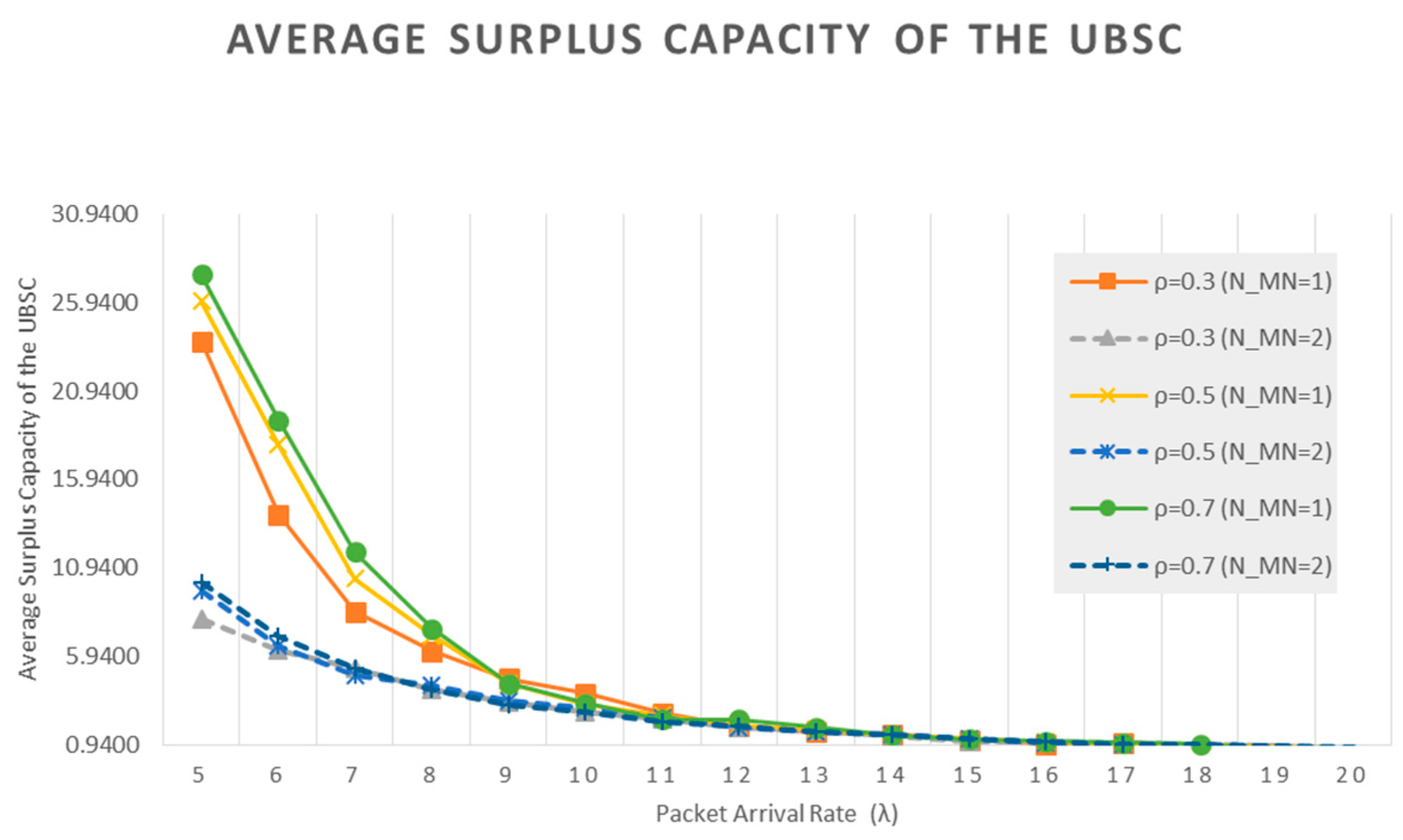
Figure 10 shows the average reserved capacity of the UBSC, denoted by for this case. We can observe that increases when the packet arrival rate is small. And it approaches to almost zero as becomes large. When is small (e.g., ), becomes larger as becomes higher and smaller. This is because a UBS returns some of its backhaul resource to the UBSC more frequently when is high, and a UBS will have a high probability to be under-utilized when is small.
4.2.2. Scenario 2
Here, we investigated the four performance measures for different adjustment parameter and the number of mobile UTs . As described in Table 3, is expressed as a function of as . We changed the value of β from 0 to 4, and that of from 1 to 2. The burst traffic, generated from each mobile UT, arrives at the UBS with Poisson arrival rate 30. And the average packet arrival rate of each UBS, denoted by , is changed from 3 to 20.
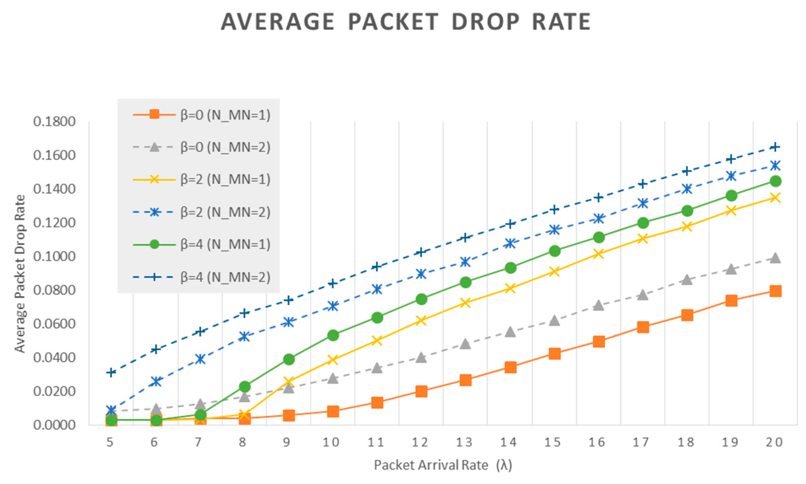
Figure 11 shows the average packet drop rate for this case. As shown in the graph, the average packet drop rate increases as the average packet arrival rate increases and the increases. In the graph, we can find that the average drop rate is different dependent upon the number of mobile nodes (or terminals) .
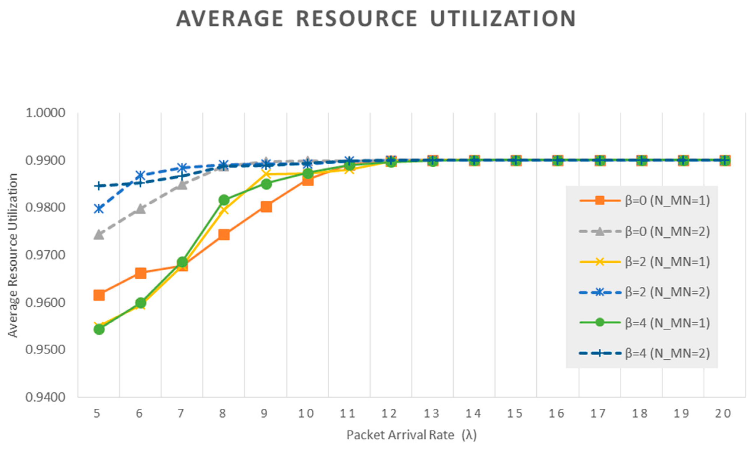
Figure 12 shows the average resource utilization for this case. As shown in the figure, the average resource utilization approaches to almost 99% as the packet arrival rate increases. Note that when = 1 and , the average resource utilization is high for , and when = 1 and , the average resource utilization is higher for and than . This can be interpreted as follows. When , the packet arrival rate of a UBS is small. So, resource utilization becomes higher for since each UBS will have 10, and this capacity can support the small packet arrival rate sufficiently. However, when , since the packet arrival rate is a little high, it requires more backhaul capacity than 10. So, by setting 12 and 14 for and , respectively, some UBSs with higher packet arrival rates than the average can have higher resource utilization.
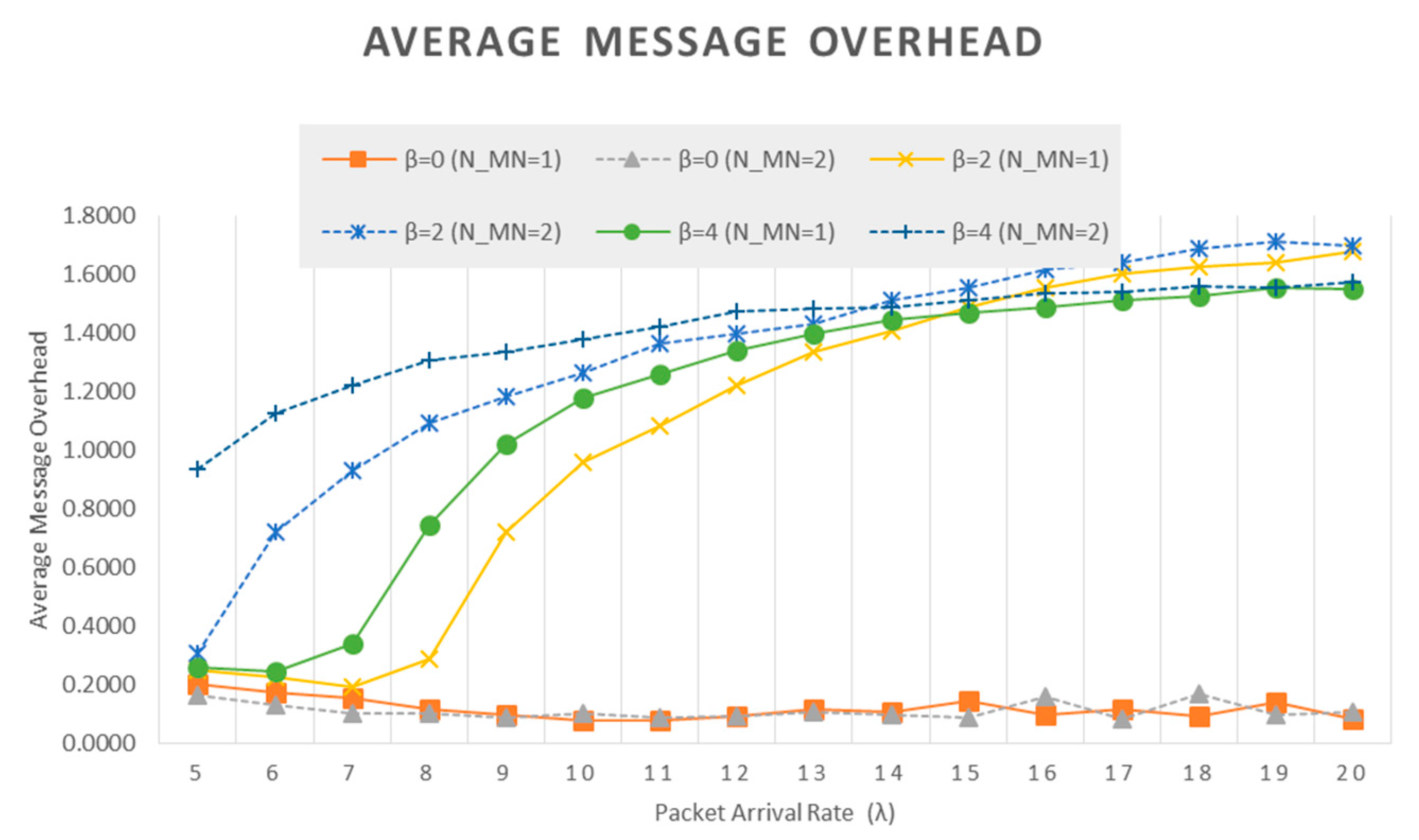
Figure 13 shows the average message overhead for this case. As shown in the graph, when , the average message overhead fluctuates within some range. However, when and , the message overhead becomes higher as the packet arrival rate increases. We can interpret this as follows. When and , each UBS can have the 12 and 14, respectively. In this case, if a UBS has large packet arrival rate compared with the other UBSs, its backhaul capacity becomes . Accordingly, the reserved capacity of the UBSC becomes small due to the limited capacity. Since we assume that the packet arrival rate of each UBS is random with Poisson distribution, some UBS with small backhaul capacity in the previous simulation interval will have high probability of packet drop. So, this will trigger the resource reallocation procedure in the UBSC, resulting in more message overhead.
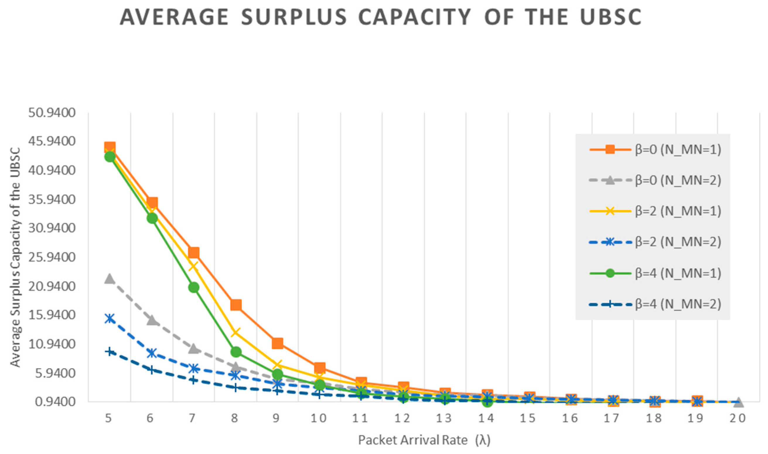
Figure 14 illustrates the average reserved capacity of the UBSC, denoted by for this case. For , we can observe that becomes larger as becomes smaller. The high value of can be interpreted in two different aspects. One is that the UBSC backhaul resource is not efficiently allocated. The other is that the high reserved capacity of the UBSC can be used to provide more capacity to the UBS with sudden burst traffic. Consequently, this will reduce the message overhead due to resource reallocation.
4.2.3. Simulation Summary
In this section, we provide a summary of our SLS results and analysis, and an operational guideline for the backhaul resource allocation in the UCWN using proposed protocol.
In our SLSs, we assumed that the total backhaul capacity of the UBSC is equal to 100 and the number of UBSs connected to the UBSC is 10. So, if the average packet arrival rate , then it would be natural that most of the UBSs suffer the shortage of the backhaul capacity. Consequently, this results in high average packet drop rate, almost peak value (i.e., nearly equal to one) for average resource utilization, and almost lowest value (i.e., approximately zero) for average reserved capacity of the UBSC. We can find this phenomenon from the graphs in Section 4.2.1 and Section 4.2.2. Therefore, in order to obtain operational guideline for the backhaul of the UCWN, we need to focus on the performance for in the SLS results.
SLS results and operational guideline for Scenario 1 can be summarized as follows.
- Average packet drop rate is not dependent upon under-utilization limit (, but more dependent upon the number of mobile UTs ( generating burst traffic and upon the average packet arrival rate .
- There is a close relationship (or a tradeoff) among the average resource utilization, the average message overhead, and the average reserved capacity of the UBSC for . Specifically, as becomes higher, the average resource utilization becomes higher, the average message overhead also gets higher, and the reserved capacity of the UBSC also becomes higher.
- This means that as becomes higher, each UBS uses only required backhaul capacity and returns unused backhaul capacity to the UBSC. Accordingly, the reserved capacity of the UBSC becomes higher. However, to maintain only required backhaul capacity in each UBS, each UBS needs to send and receive the control signaling messages, which results in high average message overhead.
- Note that high reserved backhaul capacity in the UBSC can be helpful to cope with burst traffic with high packet arrival rate in some UBSs (mainly caused by the mobile terminals such as AUVs).
SLS results and operational guideline for Scenario 2 can be summarized as follows.
- Average packet drop rate increases as the adjustment parameter ( increases. Average packet drop rate becomes higher as the average packet arrival rate and the number of mobile UTs ( increases.
- For and the number of mobile UTs ( is equal to one, the average packet drop rate is almost the same as and increase. This is because UBSs have sufficient backhaul capacities to support low packet arrival rate.
- For , there is a close relationship (or a tradeoff) among the average resource utilization, the average message overhead, and the average reserved capacity of the UBSC. Specifically, as becomes higher, the average resource utilization becomes lower, the average message overhead also gets higher, and the reserved capacity of the UBSC also becomes lower.
- This means that as becomes higher, a UBS can have higher the maximum backhaul capacity given by + . So, in this case, some UBSs can have larger backhaul capacity than (equal to 10 in the SLS) and the capacity may not be fully utilized due to small , resulting in low resource utilization. Besides, when some UBSs have larger backhaul capacity than due to > 0, the other UBSs will have lower capacity than since the total backhaul capacity is limited. Consequently, the reserved capacity of the UBSC becomes lower for larger . In this case, if the traffic pattern of the UBSs is changed, the probability that backhaul capacity for each UBS is adjusted to reflect the updated traffic condition becomes high. Thus, the average message overhead mainly due to this adjustment can be large when is large.
- For , there is a close relationship (or a tradeoff) among the average resource utilization, the average message overhead, and the average reserved capacity of the UBSC, which is different from the relationship for .
- Specifically, as becomes higher, the average resource utilization becomes higher, the average message overhead also gets higher, and the reserved capacity of the UBSC also becomes lower.
- Note that for this case as becomes higher, the average resource utilization becomes higher. This is because, for , some UBSs can have higher backhaul capacity (given by + ), and this capacity (greater than ) can handle burst traffic as well as instantaneous high traffic due to large . Consequently, the backhaul resource can be almost fully utilized, producing high average resource utilization.
- Therefore, when we determine the operational value of in the real UCWN, we first need to consider the average packet arrival rate of UBSs.
5. Conclusions
In this paper, we have discussed a new backhaul resource allocation protocol for the UCWN, where a UBS triggers to readjust its backhaul capacity with respect to its queue status: resource under-utilization or packet drops due to queue-overflow. This is quite different from the conventional resource allocation protocols in literature where a base station controller periodically assigns the backhaul capacity of base stations considering their traffic information. We believe that this new protocol may have advantages over the conventional ones, particularly in harsh communication environments like underwater where the data rate is very low and the latency of the backhaul link is very large.
In order to investigate the feasibility of the new resource allocation protocol for the UCWN, we carried out system level simulations by considering many parameters and evaluated the performance such as average packet drop rate, average resource utilization, average message overhead, and the reserved capacity of the UBSC. We showed some important simulation results and analyzed with some interpretations which can be used as operation guidelines to apply our resource allocation protocol for the UCWN.
As a future research topic, we are considering the detailed comparison between the new resource allocation protocol and the previous protocol in [17] under the same simulation conditions. It would give more valuable results and be very helpful in designing the real UCWN in the near future.
Acknowledgments
This research was supported by a grant from National R&D Projects “Development of the wide-area underwater mobile communication systems” and “Development of Distributed Underwater Monitoring & Control Networks” funded by the Ministry of Oceans and Fisheries, Korea (PMS3710, PMS3620).
Author Contributions
The authors collaborated upon designing the protocol specified in this manuscript. For the analysis of proposed protocol, Changho Yun mainly built the system level simulator, and Suhan Choi took simulation experiments, investigated several performance measures, and analyzed simulation results and performances.
Conflicts of Interest
The authors declare no conflict of interest, and the founding sponsor, the Ministry of Oceans and Fisheries, Korea, had no role in the design of the study; in the collection, analyses, or interpretation of data; in the writing of the manuscript, and in the decision to publish the results.
References
- Underwater Wireless Communication Market—Global Drivers, Opportunities, Trends, and Forecasts to 2022; Infoholic Research: Bengaluru, India, 2017; pp. 35–42. Available online: https://www.infoholicresearch.com/report/underwater-wireless-communication-market-trends-and-forecast-2016-2022/ (accessed on 25 January 2018).
- Murad, M.; Sheikh, A.; Manzoor, M.; Felemban, E.; Qaisar, S. A Survey on current underwater acoustic sensor network application. Int. J. Comput. Theory Eng. 2015, 7, 51–56. [Google Scholar] [CrossRef]
- Heidemann, J.; Ye, W.; Wills, J.; Syed, A.; Li, Y. Research challenges and applications for underwater sensor networking. In Proceedings of the IEEE Wireless Communications and Networking Conference (WCNC 2006), Las Vegas, NV, USA, 3–6 April 2006; pp. 228–235. [Google Scholar] [CrossRef]
- Yun, C.; Lim, Y. GSR-TDMA: A geometric spatial reuse-time division multiple access MAC protocol for multihop underwater acoustic sensor networks. J. Sens. 2016, 2016, 6024610. [Google Scholar] [CrossRef]
- Chitre, M.; Shahabudeen, S.; Stojanovic, M. Underwater acoustic communications and networking: Recent advances and future challenge. Mar. Technol. Soc. J. 2008, 42, 103–116. [Google Scholar] [CrossRef]
- Urick, R.J. Principle of Underwater Sound, 3rd ed.; McGraw-Hill: New York, NY, USA, 1983; ISBN 10: 0932146627. [Google Scholar]
- Akyildiz, I.F.; Pompili, D.; Melodia, T. Underwater acoustic sensor networks: Research and challenges. J. Ad-Hoc Netw. 2005, 3, 257–279. [Google Scholar] [CrossRef]
- Kim, J.H.; Im, T.H.; Kim, K.Y.; Ko, H.L. A study on the underwater base station based underwater acoustic communication systems. Proc. KICS Int. Conf. Commun. 2015, 353–354. Available online: https://www.kics.or.kr/home/kor/morgue/searchArticle.aspx?Mode=search (accessed on 24 January 2018).
- Jiang, Z. Underwater acoustic networks-Issues and solutions. Int. J. Intell. Control Syst. 2008, 13, 152–161. [Google Scholar]
- Stojanovic, M.; Freitag, L. Recent trends in underwater acoustic communications. Mar. Technol. Soc. J. 2013, 47, 45–50. [Google Scholar] [CrossRef]
- Stojanovic, M. Design and capacity analysis of cellular-type underwater acoustic communications. IEEE J. Ocean. Eng. 2008, 33, 171–181. [Google Scholar] [CrossRef]
- Labrador, Y.; Karimi, M.; Pan, D.; Miller, J. Modulation and error correction in the underwater acoustic communication channel. J. Comput. Sci. Netw. Secur. 2009, 9, 123–130. [Google Scholar]
- Stojanovic, M. Frequency reuse underwater: Capacity of an acoustic cellular network. In Proceedings of the Second Workshop on Underwater Networks (WuWNet ′07), Montreal, QC, Canada, 14 September 2007; pp. 19–24. [Google Scholar] [CrossRef]
- Nabavinejad, A.; Ghahfarokhi, S. Improving coverage and capacity in underwater acoustic cellular networks. In Proceedings of the 2013 15th International Conference on Advanced Communication Technology (ICACT), Pyeong-Chang, Korea, 27–30 January 2013; pp. 1249–1256. [Google Scholar]
- Peleato, B.; Stojanovic, M. A Channel sharing scheme for underwater cellular networks. In Proceedings of the IEEE OCEANS, Aberdeen, UK, 18–21 June 2007. [Google Scholar] [CrossRef]
- Yun, C.; Park, J.; Choi, S. Backhaul resource allocation protocol for underwater cellular communication networks. J. Korean Inst. Commun. Inf. Sci. 2017, 42, 393–402. [Google Scholar] [CrossRef]
- Biswas, S.K.; Izmailov, R. Design of a Fair Bandwidth Allocation Policy for VBR Traffic in ATM Networks. IEEE/ACM Trans. Netw. 2000, 8, 2425–2431. [Google Scholar] [CrossRef]
- Son, K.; Ryu, H.; Chong, S.; Yoo, T. Dynamic bandwidth allocation schemes to improve utilization under non-uniform traffic in Ethernet passive optical networks. In Proceedings of the 2004 IEEE International Conference on Communications (IEEE Cat. No.04CH37577), Paris, France, 20–24 June 2004; pp. 1766–1770. [Google Scholar] [CrossRef]
- Subhashini, N.; Therese, A.B. User prioritized User prioritized constraint free dynamic bandwidth allocation algorithm for EPON networks. Indian J. Sci. Technol. 2015, 8, 1–7. [Google Scholar] [CrossRef]
Figure 1.
An underwater cellular wireless network consisting of UBS controller (UBSC), underwater base stations (UBSs) and underwater terminals (UTs).
Figure 1.
An underwater cellular wireless network consisting of UBS controller (UBSC), underwater base stations (UBSs) and underwater terminals (UTs).

Figure 2.
A queue model of underwater cellular wireless networks (UCWNs).
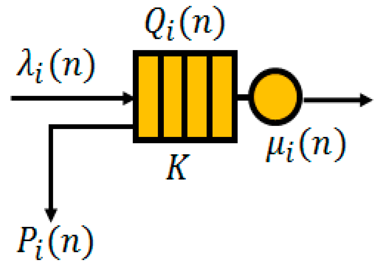
Figure 3.
The initialization phase. RIREQ: Resource Information Request; RIREP: Resource Information Response; RAIS: Resource Allocation Information Send; RAISACK: Resource Allocation Information Send Acknowledgement; NP: normal operation phase.
Figure 3.
The initialization phase. RIREQ: Resource Information Request; RIREP: Resource Information Response; RAIS: Resource Allocation Information Send; RAISACK: Resource Allocation Information Send Acknowledgement; NP: normal operation phase.

Figure 4.
Under-utilization case of the normal operation phase. IP: initialization phase; RAREQ: Resource Reallocation Request; RAACK: Resource Reallocation Acknowledgement.
Figure 4.
Under-utilization case of the normal operation phase. IP: initialization phase; RAREQ: Resource Reallocation Request; RAACK: Resource Reallocation Acknowledgement.
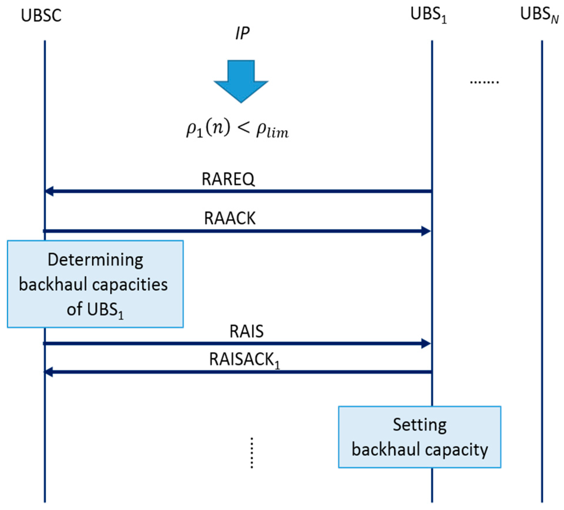
Figure 5.
Queue-overflow and sufficient reserved capacity of a UBSC case of the normal operation phase.
Figure 5.
Queue-overflow and sufficient reserved capacity of a UBSC case of the normal operation phase.

Figure 6.
Queue-overflow and insufficient reserved capacity of a UBSC case of the normal operation phase.
Figure 6.
Queue-overflow and insufficient reserved capacity of a UBSC case of the normal operation phase.

Figure 7.
Average Packet Drop Rate for different under-utilization limit ( and the number of mobile UTs (.
Figure 7.
Average Packet Drop Rate for different under-utilization limit ( and the number of mobile UTs (.

Figure 8.
Average Resource Utilization for different under-utilization limit ( and the number of mobile UTs (
Figure 8.
Average Resource Utilization for different under-utilization limit ( and the number of mobile UTs (

Figure 9.
Average Message Overhead for different under-utilization limit ( and the number of mobile UTs (
Figure 9.
Average Message Overhead for different under-utilization limit ( and the number of mobile UTs (

Figure 10.
Average Reserved Capacity of the UBSC for different under-utilization limit ( and the number of mobile UTs (.
Figure 10.
Average Reserved Capacity of the UBSC for different under-utilization limit ( and the number of mobile UTs (.

Figure 11.
Average Packet Drop Rate for different adjustment parameter (β) and the number of mobile UTs (.
Figure 11.
Average Packet Drop Rate for different adjustment parameter (β) and the number of mobile UTs (.

Figure 12.
Average Resource Utilization for different adjustment parameter (β) and the number of mobile UTs (.
Figure 12.
Average Resource Utilization for different adjustment parameter (β) and the number of mobile UTs (.

Figure 13.
Average Message Overhead for different adjustment parameter (β) and the number of mobile UTs (.
Figure 13.
Average Message Overhead for different adjustment parameter (β) and the number of mobile UTs (.

Figure 14.
Average Reserved Capacity of the UBSC for different adjustment parameter (β) and the number of mobile UTs (
Figure 14.
Average Reserved Capacity of the UBSC for different adjustment parameter (β) and the number of mobile UTs (

Table 1.
Parameters used in the underwater base station initiating (UBSI) resource allocation protocol. UBS: underwater base station; UBSC: underwater base station controller.
Table 1.
Parameters used in the underwater base station initiating (UBSI) resource allocation protocol. UBS: underwater base station; UBSC: underwater base station controller.
| Parameters | Description |
|---|---|
| The index of a UBS | |
| The number of UBSs | |
| The index of discrete time | |
| The maximum queue length | |
| The UBSC capacity | |
| The maximum backhaul capacity of a UBS | |
| The backhaul capacity of UBS at time | |
| The input traffic rate of UBS at time | |
| The reserved capacity of a UBSC at time | |
| The queue length of UBS at time | |
| The number of packet drops of UBS at time | |
| The resource utilization of UBS at time | |
| The message overhead of UBS at time |
Table 2.
Messages of the UBSI resource allocation protocol. RIREQ: Resource Information Request; IP: initialization phase; NP: normal operation phase; RIREP: Resource Information Response; RAIS: Resource Allocation Information Send; RAISACK: Resource Allocation Information Send Acknowledgement; RAREQ: Resource Reallocation Request; RAACK: Resource Reallocation Acknowledgement.
| Type | Direction | Phase | Transmission Type | Note |
|---|---|---|---|---|
| RIREQ | UBSC→UBS | IP, NP | Broadcast | Request traffic information (commonly used in IP and NP) |
| RIREP | UBS→UBSC | IP, NP | Unicast | Send traffic information (commonly used in IP and NP) |
| RAIS | UBSC→UBS | IP, NP | Unicast/Broadcast | Send the backhaul capacity to UBSs (commonly used in IP and NP) |
| RAISACK | UBS→UBSC | IP, NP | Unicast | An acknowledgement of RAIS (commonly used in IP and NP) |
| RAREQ | UBS→UBSC | NP | Unicast | Request of resource readjustment of a UBS (used in only NP) |
| RAACK | UBSC→UBS | NP | Unicast | An acknowledgement of RAACK (used in only NP) |
Table 3.
Parameters used in the System Level Simulations.
| Parameters | Description | Values in SLS |
|---|---|---|
| M | The number of SLSs with the same parameters | 10 |
| The index of discrete time per one SLS | 0~10,000 | |
| The number of UBSs | 10 | |
| The maximum queue length | 100 | |
| The capacity of a UBSC | 100 | |
| The maximum backhaul capacity of a UBS | + | |
| Adjustment parameter | 0~5 (default: 0) | |
| The backhaul capacity of UBS at time | 0 < < | |
| Average packet arrival rate of a UBS generated from normal UTs | 3~20 | |
| Under-utilization limit | 0.3~0.8 (default: 0.5) | |
| The number of mobile UTs (or nodes) generating burst traffic | 1~4 (default: 1) | |
| Average packet arrival rate of a UBS generated from mobile UTs | 10~60 (default: 30) | |
| Window size for average traffic calculation | 1~10 (default: 1) |
© 2018 by the authors. Licensee MDPI, Basel, Switzerland. This article is an open access article distributed under the terms and conditions of the Creative Commons Attribution (CC BY) license (http://creativecommons.org/licenses/by/4.0/).
Share and Cite
MDPI and ACS Style
Yun, C.; Choi, S. A New Resource Allocation Protocol for the Backhaul of Underwater Cellular Wireless Networks. Appl. Sci. 2018, 8, 178. https://doi.org/10.3390/app8020178
AMA Style
Yun C, Choi S. A New Resource Allocation Protocol for the Backhaul of Underwater Cellular Wireless Networks. Applied Sciences. 2018; 8(2):178. https://doi.org/10.3390/app8020178
Chicago/Turabian StyleYun, Changho, and Suhan Choi. 2018. "A New Resource Allocation Protocol for the Backhaul of Underwater Cellular Wireless Networks" Applied Sciences 8, no. 2: 178. https://doi.org/10.3390/app8020178
Note that from the first issue of 2016, this journal uses article numbers instead of page numbers. See further details here.