Uncertainty Propagation of Spectral Matching Ratios Measured Using a Calibrated Spectroradiometer


Directorate C—Energy, Transport and Climate, European Commission Joint Research Centre, I-21027 Ispra, Italy
*
Author to whom correspondence should be addressed.
Appl. Sci. 2018, 8(2), 186; https://doi.org/10.3390/app8020186
Submission received: 29 November 2017
/
Revised: 17 January 2018
/
Accepted: 19 January 2018
/
Published: 26 January 2018
(This article belongs to the Special Issue Next Generation Photovoltaic Solar Cells)
Abstract
:Featured Application
The results of this paper are needed in the calculation of measurement uncertainty associated with the performance of Concentrator Photovoltaic (CPV) devices, in particular for measurements taken outdoors. As of today’s state-of-the-art capability in measuring CPV devices, outdoor measurements are the most reliable.
Abstract
The international standard IEC62670-3 (International Electrotechnical Committee) “Photovoltaic Concentrators (CPV) Performance Testing—Part 3—Performance Measurements and Power Rating” sets the guidelines for power measurements of a CPV device, both in indoor and outdoor conditions. When measuring in outdoor conditions, the acquired data have to be filtered a posteriori, in order to select only those points measured with ambient conditions close to the Concentrator Standard Operating Conditions (CSOC). The most stringent requirement to be met is related to the three Spectral Matching Ratios (SMR), which have all to be within the limit of 1.00 ± 0.03. SMR are usually determined by the ratio of the currents of component cells to monitor the outdoor spectral ratio conditions during the CPV device power measurements. Experience demonstrates that obtaining real world data meeting these strict conditions is very difficult in practice. However, increasing the acceptable range would make the entire filtering process less appropriate from a physical point of view. Given the importance of correctly measuring the SMR, an estimation of their associated measurement uncertainties is needed to allow a proper assessment of the validity of the 3% limit. In this study a Monte Carlo simulation has been used, to allow the estimation of the propagation of uncertainties in expressions having the and integral form. The method consists of applying both random and wavelength correlated errors to the measured spectra and to the measured spectral responses of the three CPV cell junctions, according to the measurement uncertainties of the European Solar Test Installation (ESTI). The experimental data used in this study have been acquired during clear sky conditions in May 2016, at ESTI’s facilities in Ispra, northern Italy (45°49′ N 8°37′ E).
1. Introduction
Concentrator photovoltaics (CPV) occupy a small niche of the global photovoltaic (PV) market. However, several power plants with capacity of more than 30 MWp have been realized, mainly in China and in the U.S., with a total installed capacity of about 360 MWp already grid-connected [1]. Even though manufacturing capacity has recently decreased worldwide, mainly due to the unprecedented rapid drop of crystalline silicon prices, CPV technology remains very promising: the highest efficiency values for concentrator multi-junction cells reached 46.0 ± 2.2% at 508 suns and the scientific outlook is robust [2]. However, in order to be competitive with Crystalline silicon (c-Si) technology CPV has to increase system efficiency to at least 40%, and concentration ratios up to 1000×, according to [3]. Given that the price depends on the rated power, as is the case for flat-plate modules, reliable measurements of maximum power (and consequently of the efficiency) are crucial. In 2017 the international standard IEC62670-3 “Photovoltaic concentrators (CPV)—Performance testing—Part3: Performance measurements and power rating” [4] was published; it specifies different methods to measure the electrical characteristics of CPV devices both indoor and outdoor. In order to explore the standard’s applicability, several measurements on a triple-junction CPV cell have been performed at the European Solar Test Installation (ESTI) of the European Commission’s Joint Research Centre, located in Ispra, northern Italy (45°49′ N 8°37′ E). Some preliminary results have already been presented and published in a previous work [5]. The approach for outdoor measurements is to acquire current-voltage (IV) curves of the CPV device under clear sky conditions, together with the relevant meteorological quantities at ground level and the direct normal spectral irradiance with simultaneous acquisitions throughout the day. Subsequently filtering is applied to the acquired data in order to reduce the data set only to the points near Concentrator Standard Operating Conditions (CSOC) conditions, defined in [6], which the IV curves have been translated to. The most stringent requirement is related to the spectral match between the reference spectrum AirMass 1.5 Direct (AM1.5D) and the measured spectrum at time t, which is determined by calculating the three spectral matching ratios SMR12, SMR13, SMR23, which must lie in the interval 1.00 ± 0.03 in order for the measured IV curve to be valid (in this notation 1 denotes the top, 2 the middle and 3 the bottom cell). This limit is specified in the standard and has an impact on the final calculated performance of the CPV device: A larger interval would have the advantage of an increased statistical population size, with the disadvantage that points far from the target CSOC conditions would be considered in the calculation. However, this stringent acceptance limit makes sense only if the measurement uncertainty of each SMR is much less than the limit itself. In the present study the uncertainty sources of the SMR quantities are considered, using real data from the ESTI calibration chains and data acquired in-the-field, in order to estimate the uncertainties of each SMR by a Monte Carlo simulation. Each run of the algorithm consisted in 100,000 iterations, in order to generate a sufficient number of random errors which are added to the measured quantities. The resulting values are then compared to the acceptance threshold prescribed in the standard.
2. Measurement Method
The spectral matching ratios SMR are defined as the short circuit current ratios between two junctions normalized to the short circuit currents produced under the reference condition AM1.5D:
The calculated (SMR for simplicity) is a function of time because the solar spectrum changes during the day, affecting the first term, while the second term is a function only of the spectral responses of the two junctions and of the reference spectrum, so is constant. As a ratio of four currents, the SMR is a dimensionless value.
There are two methods most frequently used to measure the SMR: by making use of a calibrated spectroradiometer or by using component cells, each having spectral responsivities representative of the actual multi-junction devices [4].
The latter approach is simpler in terms of operation, because it does not need a complex calibrated (and hence expensive) spectroradiometer system to continuously measure the spectral irradiance. Moreover the three spectral responsivities of the CPV device under test do not have to be measured. However, a good result is guaranteed only if matched component cells are used and after a proper calibration. If this is not the case, this method furnishes an approximate measurement only.
The present study uses only the spectroradiometer method, and the short circuit currents are calculated by
By substituting Equations (2) and (3) into Equation (1) we obtain
Equation (4) highlights the remarkable symmetry property of the SMR with respect to all the four functions , , and : A linear transformation of one or more of the four functions of form
has no impact on the SMR. In other words, the SMR does not depend on the magnitude of the measured curves, but only on their relative shape.
3. Sources of Uncertainty
The uncertainties associated with the three SMR depend on the uncertainties of the quantities in the four integrals in Equation (4). All of them are experimentally measured quantities except for the reference spectrum , which is tabulated in [7] with no associated uncertainty. It is important to note that in order to perform the multiplication of two functions, they have to be defined on the same abscissa. In general, a spectral response curve (measured using narrow band-pass filters), a spectral irradiance (measured with a grating spectroradiometer), and the reference spectrum are all tabulated on different wavelengths. As a consequence, a suitable interpolant has to be used to define all the functions on the same nodes. In the present study a piecewise cubic Hermite polynomial has been used as interpolant, because it offers a better control of the first derivative of the function. In general, the interpolation error is limited by [8]:
A detailed analysis of the interpolation error can be neglected in the present study, because by observing Equation (6) it may be seen that it is one of the smallest sources of uncertainty; it would not be negligible only in the case of functions with very few measured points and large derivatives, interpolated on a coarse grid of nodes, which is not the case here: The spectral responsivities are measured at intervals of 20–30 nm distance from one point to the adjacent one, while the spectra at non-uniform intervals of about 1 nm. A possible effect due to interpolation will appear in the spectral responsivity sensitivity analysis, which highlights some non-linearity at very small values, due to the fewer number of measured points, compared to the same analysis conducted on the spectrum which is measured with a fine step size. In the implementation of the Monte Carlo method, it is essential to first associate the random error to all the measured points individually, and only afterwards perform the interpolation; associating the errors to the interpolated points would lead to incorrect results.
3.1. Uncertainty Budget Associated with the Spectral Responsivity
The spectral responsivity of multi-junction devices is performed at ESTI according to standard IEC60904-8-1(2017), with suitable bias light to saturate the junction(s) not under measurement and narrow band light at wavelengths where the junction under measurement responds. Both the device under test and the reference device are over-illuminated, including not only active area, but also cover and package. The narrow band light is obtained from a broadband xenon light source filtered by interferential bandpass filters with bandwidth from 10–20 nm full-width-half-maximum (FWHM), covering the wavelength range of 300 to 1900 nm. The quasi-monochromatic light is then chopped at a fixed frequency, and the short-circuit current signal is measured by lock-in amplifiers, which enable extraction of the signal due to the quasi-monochromatic light from the static component due to the bias lights [9]. The narrow band light simultaneously illuminates the device under test and the reference device; the spectral response of the device under test is calculated from the ratio of the two device currents.
The following principal components contribute to the uncertainty of the spectral responsivity:
- Electrical uncertainty (lock-in amplifiers, current-voltage converters, experimental noise)
- Temperature uncertainty (measurement conditions at 25.0 ± 1.0 °C and thermometers calibrations)
- Optical uncertainty (the spatial non-uniformity of quasi-monochromatic light on the measurement plane, alignment of device under test and reference device, area of device under test and reference)
- Reference cell uncertainty (calibration and drift)
The electrical standard uncertainty due only to the lock-in amplifiers and the current-voltage converters is ±0.56%, excluding the electrical noise contribution, which is measured during each acquisition by the standard deviation of the signal ratios as each wavelength point is measured a number of times. This value varies with wavelength and device. The temperature of the device and of the reference cell is controlled during the measurement by two separate base plates, controlled by a water circuit and by a Peltier element respectively. The temperature standard uncertainty contribution, considering both items, amounts to ±0.06% and is the smallest of the four uncertainty components. The two devices are kept as physically as close as possible, but nevertheless non-uniformity of the incident quasi-monochromatic light is unavoidable, due to the non-uniformity of the Xenon light source itself and of the filters; each filter generates a different uniformity pattern on the test area. Considering the worst case, the standard non-uniformity uncertainty is ±1.16% for small area reference cells (typically 400 mm2). Given that the two devices are placed on two different plates, a tilt alignment error within 2° is assumed, corresponding to a standard uncertainty of ±0.03%. The last component of the optical uncertainty budget is due to the area of the devices, which enters in the calculation of the ratio of the short-circuit current ratio, and which has to be normalized to the unit area. The area is measured by a calibrated meter equipped with a magnification camera, traceable to SI Units with a standard uncertainty of ±0.07%. The area contribution is excluded in the present exercise because it does not influence the SMR (see Equation (5)). The final values of the spectral responsivity (SR) uncertainty are therefore due to some components which are independent of wavelength and others that are wavelength-dependent (the calibration uncertainty of the reference cell and the electrical noise component). An example of measured spectral responsivity curves of the three junctions together with associated standard uncertainties is shown in Figure 1.
3.2. Uncertainty Budget Associated with the Spectrum Measurement
The uncertainty budget of the spectrum measurement is composed of the following items:
- Standard lamp calibration uncertainty and drift
- Internal calibration transfer uncertainty
- Temperature control of the detectors in outdoor conditions
As already explained, the SMR depends only on the shape of the measured curves, so systematic effects affecting uniformly all the wavelengths do not impact the SMR uncertainty; for example, since all the devices are placed on the same solar tracker, possible tracking errors have not to be taken into account in the uncertainty budget.
The spectroradiometer used in the present study has been internally calibrated against a standard lamp, calibrated at NPL (National Physical Laboratory UK). Uncertainty arises mainly from calibration, including uncertainty of calibration laboratory and expected lamp calibration drift. Average NIST irradiance scale standard uncertainty is ±0.70%, with calibration laboratory transfer accounting for another ±0.55%. During 50 h of operation, the lamp drift is estimated to be ±1.00%; if this is considered the limit of a rectangular distribution, the associated standard uncertainty is ±0.59%. The uncertainty of the standard lamp is then transferred to the spectroradiometer via periodic internal recalibrations. During the process the main uncertainty components are stray light, lamp to spectroradiometer entrance slit distance, lamp current and lamp orientation. Stray light contribution is estimated to be ±0.29%, even with blackened walls and surfaces, and no object in the room being at a distance less than 1.5 m from the optical table. The distance lamp–spectroradiometer is set by a 500 mm calibrated gauge block; a residual uncertainty in the lamp distance is estimated to be within ±0.5 mm, leading to a standard uncertainty in the irradiance spectral intensity of ±0.10%. The spectral distribution of the lamp is affected by the current injected into the lamp during calibration of the spectroradiometer. Uncertainty of the power supply is due to the instrument resolution and long-term drift; however these terms combined account for a standard uncertainty contribution of only ±0.03%.
During outdoor operation the two detectors (c-Si for the range 300–1150 nm and InGaAs until 1700 nm) are temperature controlled by separate Peltier elements inside the instrument case. However, a temperature gradient between the temperature read by the feedback sensor and the true junction temperature might be possible, depending upon the position of the temperature sensors inside the instruments. If the real temperature differs from the temperature at which the instrument was calibrated, the current produced by the detectors changes, due to the change of spectral responsivity of crystalline silicon and InGaAs materials with temperature. This contribution is modeled in the Monte Carlo method, by shifting the portion of spectral irradiance in the following wavelength intervals [10]:
Finally, as an empirical check of the input uncertainties estimation, the expanded uncertainty (k = 2) of the spectral irradiance measurement have been compared with the deviations with respect to the average spectrum of 14 consecutive acquisitions of a steady-state solar simulator Xenon lamp. Approximately 95.45% of the points were within the uncertainty limits as expected providing a verification of the uncertainties.
4. Results
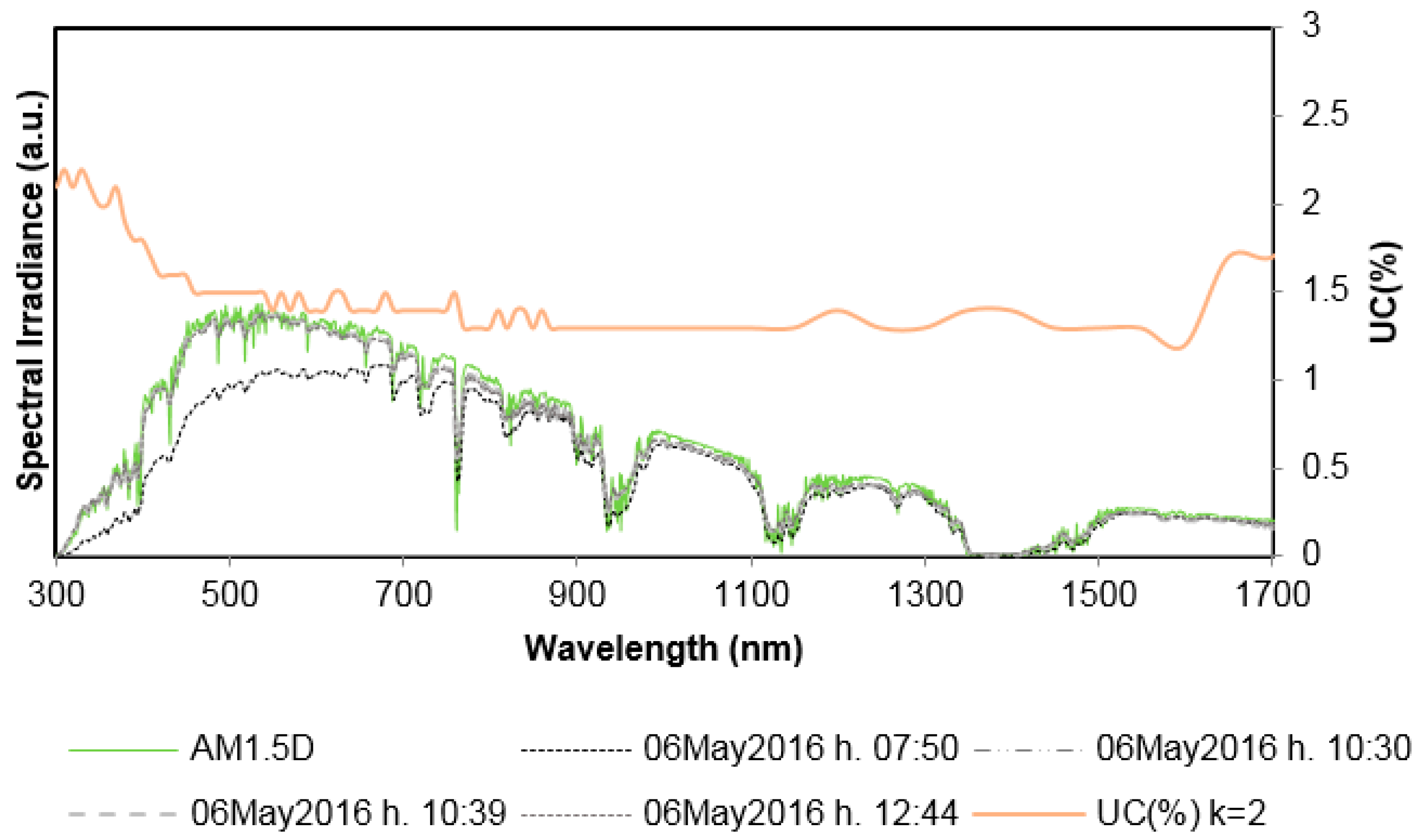
The standard uncertainties of the three SMR have been calculated as the standard deviations of the associated probability density functions [11]. The sensitivity analysis of the various sources of error was performed running the Monte Carlo simulation on four different spectra measured during the 6 May 2016 at Ispra, ranging from the early morning to the early afternoon. Four spectra have been chosen for the analysis, and they are plotted in Figure 2 together with the AM1.5D reference spectrum. Three of the spectra result in SMR values within the 3% acceptance limit, while the first acquired spectrum of the day would clearly give results outside the limit, because of its low UV and visible content (Figure 3). It was included in this analysis to check that the results are applicable also to spectra very different from from AM1.5D conditions. The uncertainty wavelength-dependent function is also shown.
4.1. Contribution of Spectral Responsivity Errors
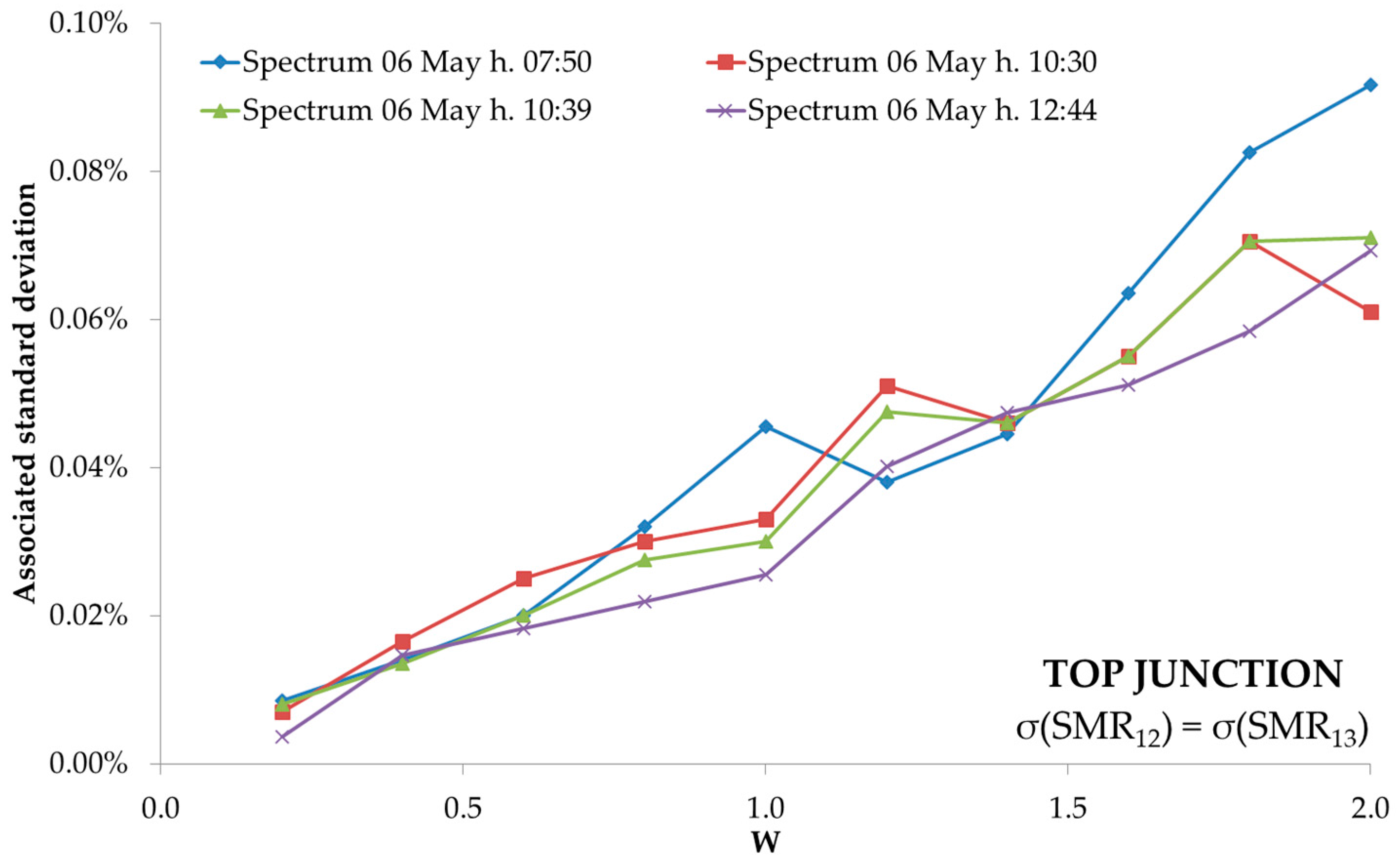
The errors on every junction spectral responsivity measurements affect only the SMR in which the junction is involved in; as an example, errors on the top junction do not affect SMR23. Moreover, the two affected SMR are equal, because in this sensitivity analysis all the contributions are considered separately. For each measured spectrum, the function associated to the considered junction has been multiplied by a coefficient w (0.2 ≤ w ≤ 2), to study the sensitivity of the output errors varying the absolute values of the input errors. The case w = 1 describes the case in which the ESTI declared uncertainty are used in the simulation.
This approach gives not only a value of the error of the output quantity given the actual input errors, but also how sensitive it is to them: The more the output quantity is sensitive to input variations, the more important it is that the input errors must be precisely estimated. The following figures show the results of the three junctions individually considered.
The top junction is considered in Figure 4: it can be seen that even doubling the declared uncertainty on the top junction the standard deviation of SMR12 and SMR13 remain below 0.10%. The case w = 1 leads to a standard deviation of 0.05%.
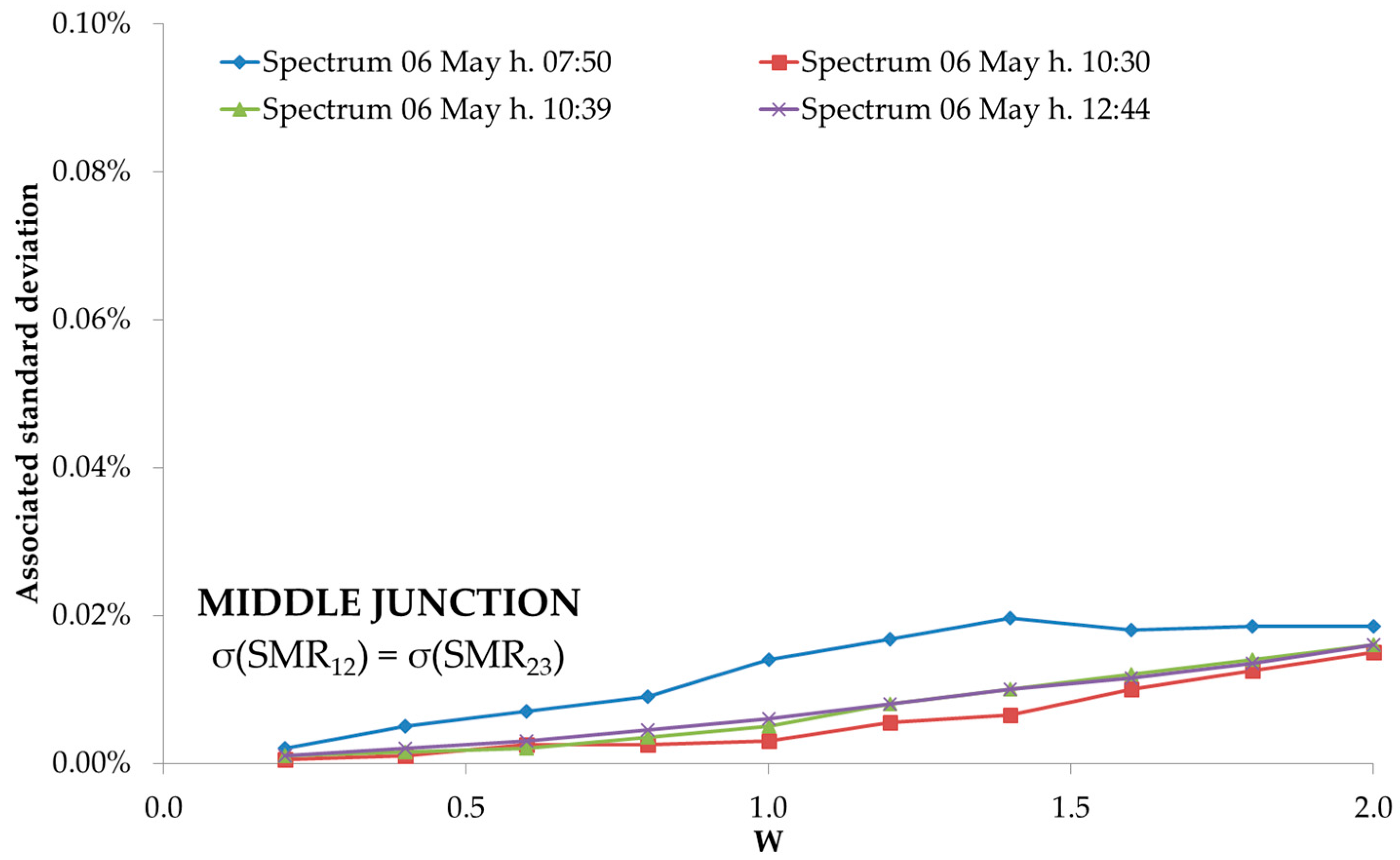
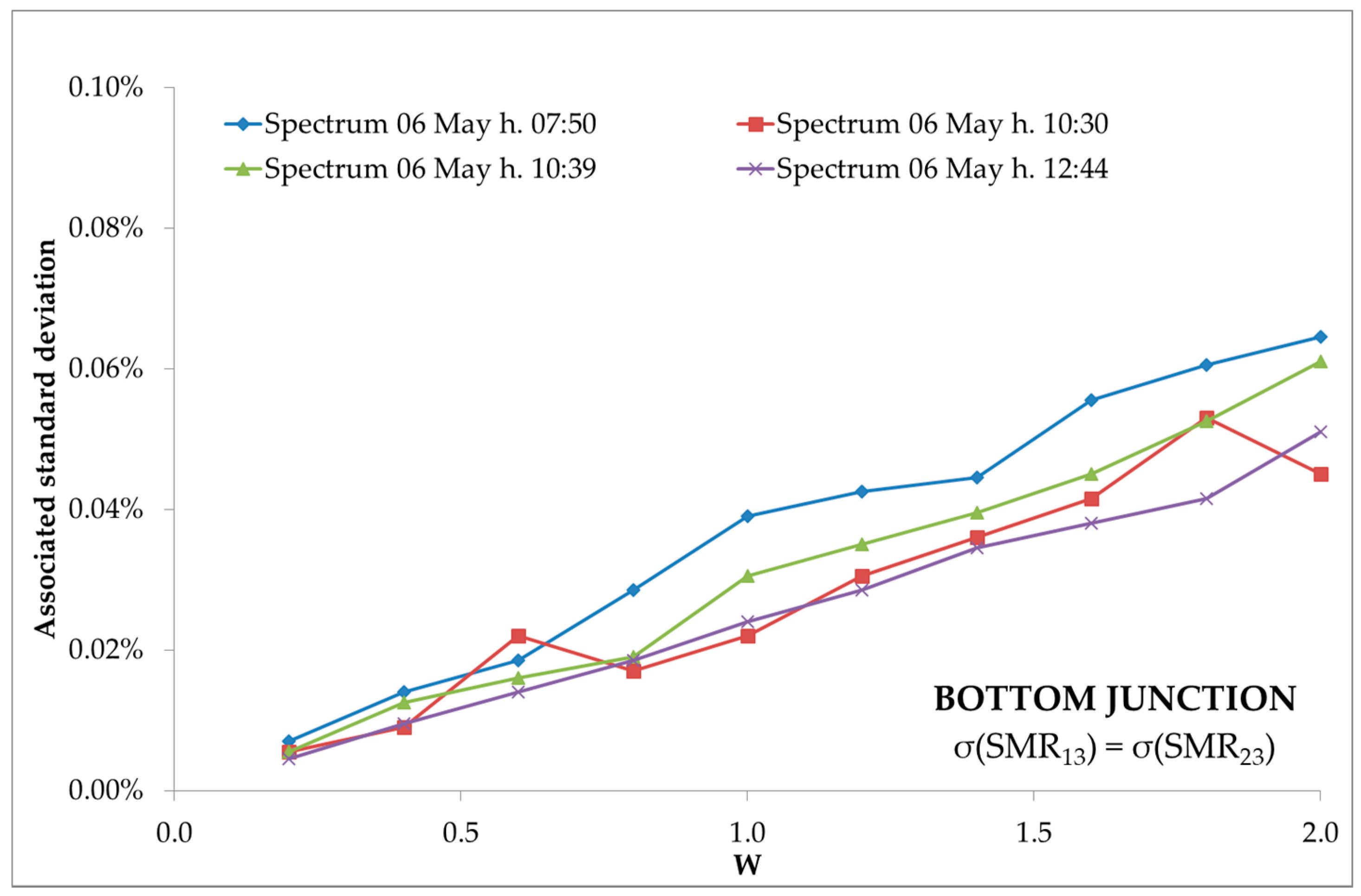
For the middle junction (Figure 5) the standard deviation is 0.015% in the special case w = 1, and SMR12 and SMR23 are less dependent upon the errors on the middle junction spectral responsivity (the slope is lower). Finally, the errors on the bottom junction result in a standard deviation of 0.04% for the case w = 1 (Figure 6).
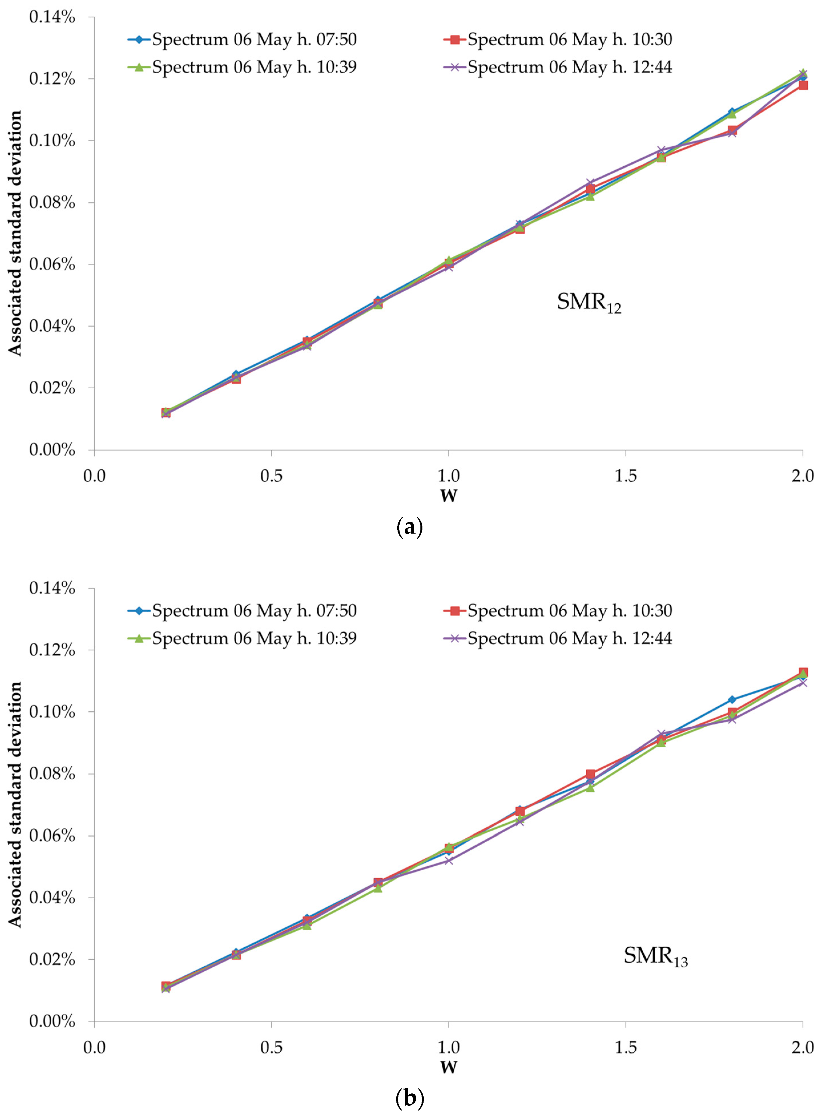
4.2. Contribution of Random Errors on Measured Spectrum
In the previous section the contributions of Top, Middle and Bottom junctions spectral responsivities have been analyzed. The other source of uncertainty comes from the measured spectrum which, in the case of this study, is measured by a grating spectroradiometer with two detectors having different spectral ranges (crystalline silicon and InGaAs). The final spectrum is the combination of the two. The uncertainties listed in Section 3.2 act as random variables, for which there is no correlation between their values at adjacent wavelengths. The effect of the integral operator is then to smooth the variability of the output integral quantity. Moreover, the SMR function is invariant in respect with multiplication, so absolute errors acting on all the wavelengths by the same amount do not affect the final value. The approach is the same of the spectral responsivity impact study: the uncertainty function declared by ESTI is multiplied by a factor w, within the range of interest 0.2 ≤ w ≤ 2. As can be seen in Figure 7 the impact of random errors on spectrum is evidently smoothed by the integral operator. The impact on the three SMR is comparable to the second decimal digit (order of 0.01%). The case w = 1 suggests an overall uncertainty contribution of about 0.06% (k = 1), for all the three cases.
4.3. Contribution of Temperature Errors on Measured Spectrum
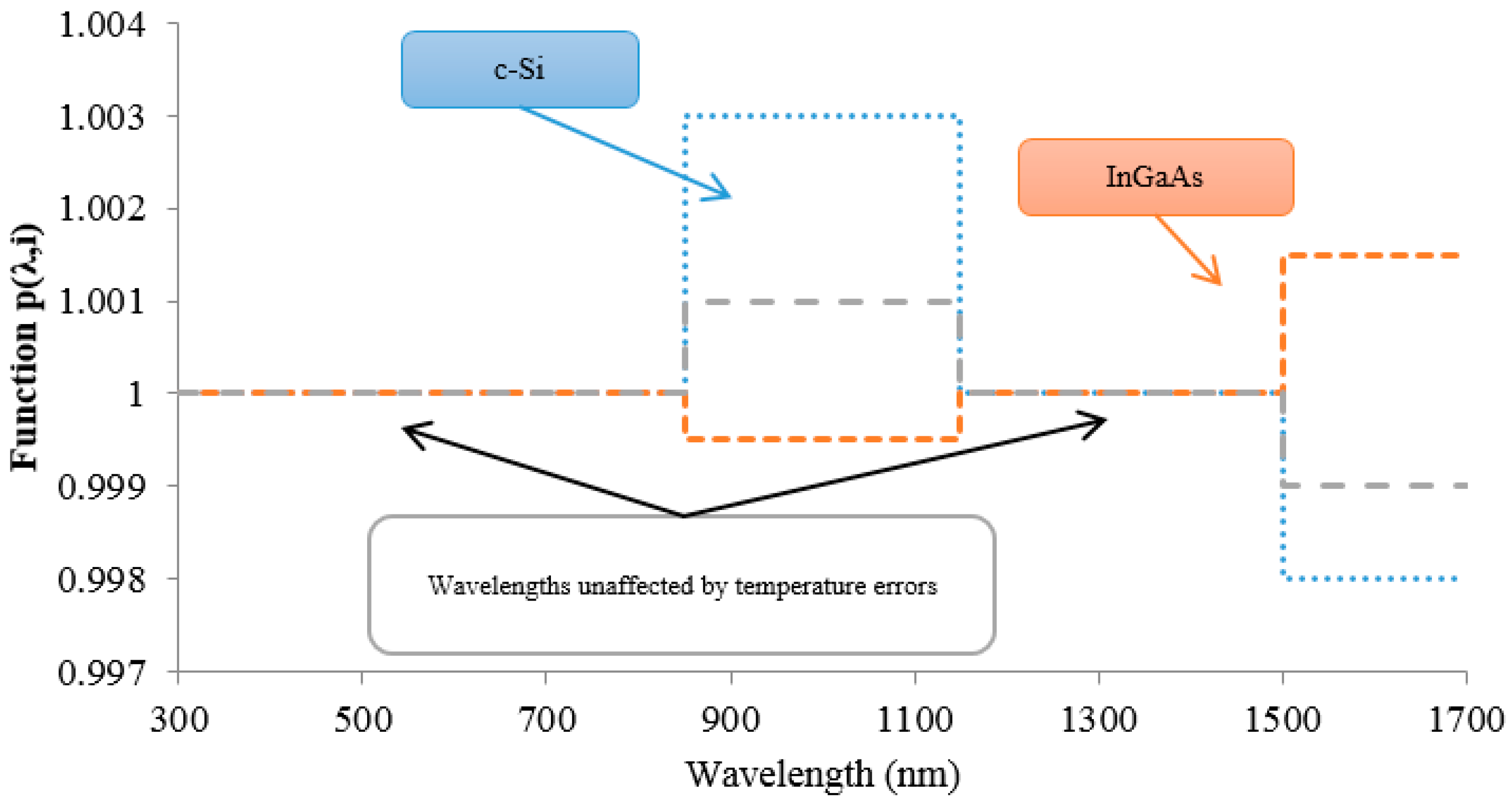
As already described, the direct normal spectral irradiance is measured using a calibrated grating spectroradiometer with two detectors. The measurement has to be performed maintaining both detectors at the same temperature at which the calibration of the spectroradiometer was performed. The sensors have their temperature controlled by two separate Peltier elements, but the measured temperature differs from the effective junction temperature, due to the position of the temperature sensor with respect to the detector, to the irradiance variability during the measurement, and to the exposition of the spectroradiometer body to the outdoor conditions. The effect of this uncertainty has to be estimated; in the present study it is modeled with a Gaussian distribution with ±1.5 °C. The uncertainty associated with the temperature of the two sensors does not affect all the wavelengths, but only the intervals specified in Equation (7) [10]. The algorithm to adjust the measured spectra is
where the function p acts as a weighting factor only in the regions 850 ≤ λ ≤ 1150 nm and 1500 ≤ λ ≤ 1700 nm, otherwise it is unity. The index (i) in Equation (8) refers to the trial number, because the function changes at each iteration following the Gaussian of all the possible values of temperature errors. The two Gaussian curves modeling crystalline silicon and InGaAs temperature errors are independently generated. An example is shown in Figure 8.
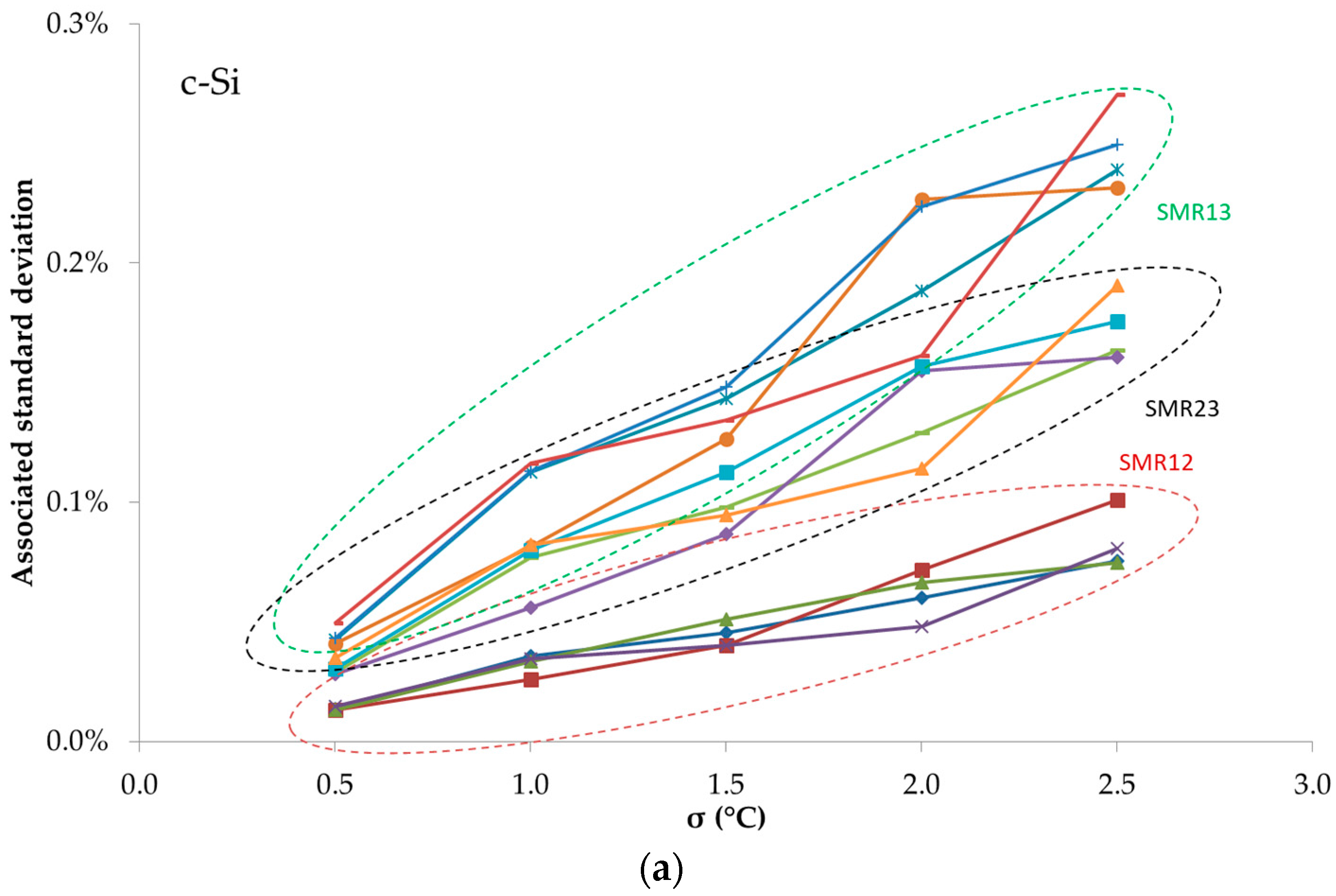
In order to study the uncertainty component associated with each of the two temperature errors, the factors of c-Si and InGaAs have been used alternately, varying the amplitude of the Gaussian probability:
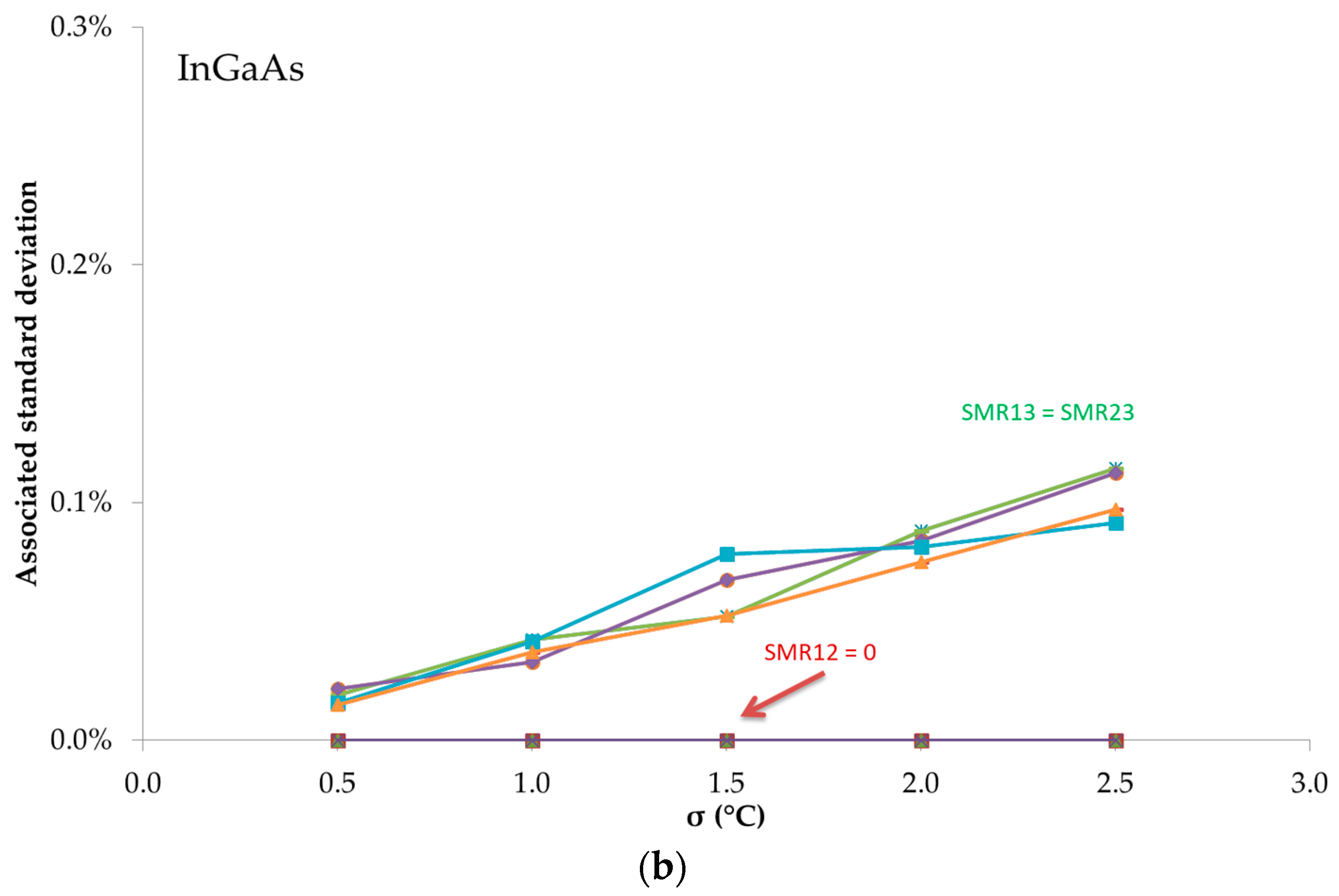
The results are shown in Figure 9 for c-Si and InGaAs separately, considering the different spectra. The c-Si temperature error affects all the three SMR, because it is present in both the Top and Middle junctions; the magnitude of the variation of the three SMR depends on the values of spectral irradiance and spectral responsivities in the interval [850; 1150] nm. Regarding the variation associated with error in InGaAs, only the bottom junction responds in the wavelength range from 1500 to 1700 nm. Therefore, only SMR13 and SMR23 are affected, and by the same amount, because the error source is the same.
Considering the estimated σ = ±1.5 °C the corresponding output standard deviations are summarized in Table 1.
4.4. Overall Uncertainties
The overall uncertainty is due to the superposition of all the contributions separately analyzed in the previous sections. The specific cases involving the ESTI input uncertainties have to be considered all together in a single run of the Monte Carlo method. The simulation is then performed for all the different measured spectra, to assess the stability of the result upon different irradiance levels and spectral distributions. The results of the Monte Carlo method with all the different degrees of freedom are summarized in Table 2 and compared with the result obtained by a straightforward sum of squares calculation.
5. Conclusions
According to the International Standard IEC 62670-3 the data of power performance of CPV devices measured outdoors have to be filtered in order to restrict the set only to those points close to the Concentrator Standard Operating Conditions. The strictest requirement is that all the three Spectral Matching Ratios (SMR) must be in the range 1.00 ± 0.03, to eliminate points acquired with spectral conditions too far from the reference spectrum. The present study calculated, using a Monte Carlo method, the uncertainties associated with the three SMR measured using a calibrated spectroradiometer and the measured spectral responses of the triple-junction CPV device. The values of the expanded (k = 2) uncertainties are one order of magnitude less than the limit, with the highest value of ±0.42% for SMR23, and hence the 3% value is meaningful for this measurement method. However, the uncertainties of solar spectrum and spectral response measurements at ESTI are representative of only a few top-class laboratories in the world, and hence typical uncertainties on SMR are expected to be generally higher. It is advisable for each laboratory dealing with outdoor power measurements of CPV devices to declare also the specific uncertainties of the SMR used to filter the acquired data. The uncertainties of SMR calculated using an isotype component cell has not been considered in this study, but the fact that the isotype device sub-junctions are generally different to the particular device under test leads to an approximate method.
Acknowledgments
The present work has been funded by the European Commission Directorate General Joint Research Centre, in the framework of the Horizon 2020 programmes. The European Commission granted also for the Open Access to this paper.
Author Contributions
Diego Pavanello conceived this work, and for this work he was responsible for the design and implementation of the Monte Carlo analysis and he wrote the paper. Roberto Galleano is the responsible of metrology laboratory at ESTI, and for this work he contributed with uncertainty analysis of solar spectrum measurements. Robert P. Kenny is responsible of the concentrator photovoltaic activities at ESTI, and manages the outdoor setup measurement system. Authors would like to highlight the contribution of Harald Müllejans in the review phase of this article.
Conflicts of Interest
The authors declare no conflict of interest.
Abbreviations
| Wavelength | |
| Spectral Mismatch Ratios between junctions i and k (i, k = 1…3, i ≠ k) | |
| Spectral responsivity of i-th junction | |
| Spectral irradiance measured at time t | |
| Reference spectral irradiance AM1.5D | |
| Short circuit current produced by junction i (i = 1…3) at time t | |
| Short circuit current produced by junction i (i = 1…3) with reference spectrum | |
| Standard uncertainty associated to a quantity | |
| Combined uncertainty associated to a quantity | |
| Expanded uncertainty associated to a quantity | |
| Hermite interpolant of the function f(x) on the nodes xi |
References
- Philipps, S.; Horowitz, K.; Kurtz, S. Current Technology Status of Concentrator Photovoltaic (CPV); Fraunhofer Institute for Solar Energy Systems ISE: Freiburg, Germany, 2016. [Google Scholar]
- Green, M.A.; Emery, K.; Hishikawa, Y.; Warta, W.; Dunlop, E.D.; Levi, D.H.; Ho-Baillie, A.W.Y. Solar cell efficiency tables (version 49). Prog. Photovolt. Res. Appl. 2017, 25, 3–13. [Google Scholar] [CrossRef]
- Ekins-Daukes, N.J.; Sandwell, P.; Nelson, J.; Johnson, A.D.; Duggan, G.; Herniak, E. What does CPV need to achieve in order to succeed? AIP Conf. Art. 2016, 1776, 20004. [Google Scholar]
- International Electrotechnical Committee (IEC). International Standard IEC62670-3, 1st ed.; IEC International Electrotechnical Committee: Geneva, Switzerland, 2017. [Google Scholar]
- Pavanello, D.; Galleano, R.; Kenny, R.; Müllejans, H.T. Uncertainty Propagation of Spectral Matching Ratios Measured Using a Calibrated Spectroradiometer. In Proceedings of the 13th European photovoltaic solar energy conference proceedings, Amsterdam, The Netherlands, 25–29 September 2017. [Google Scholar]
- International Electrotechnical Committee (IEC). International Standard IEC 62670-1, 1st ed.; IEC: Geneva, Switzerland, 2013. [Google Scholar]
- International Electrotechnical Committee (IEC). International Standard IEC60904-3, 3th ed.; IEC: Geneva, Switzerland, 2013; Volume 2016. [Google Scholar]
- Alfio, Q.; Riccardo, S.; Fausto, S. Matematica Numerica; Springer Science & Business Media: Berlin, Germany, 2000. [Google Scholar]
- International Electrotechnical Committee (IEC). International Standard IEC60904-8, 3th ed.; IEC: Geneva, Switzerland, 2014; Volume 2014. [Google Scholar]
- Ma, Y.; Zhang, Y.; Gu, Y.; Chen, X.; Xi, S.; Du, B.; Li, H. Tailoring the performances of low operating voltage InAlAs/InGaAs avalanche photodetectors. Opt. Express 2015, 23, 19278–19287. [Google Scholar] [CrossRef] [PubMed]
- Woolliams, E.R. Determining the Uncertainty Associated with Integrals of Spectral Quantities; European Association of National Metrology Institutes: Berlin, Germany, 2013. [Google Scholar]
Figure 1.
Spectral responsivity (SR) curves of the three junctions (continuous lines, left axis) with their wavelength-dependent associated standard uncertainties UC (dotted lines, right axis); the peaks are due to the fact that high relative errors occur at very low currents and poor signal/noise ratio. The functions shown in figure are those interpolated with a 1 nm step.
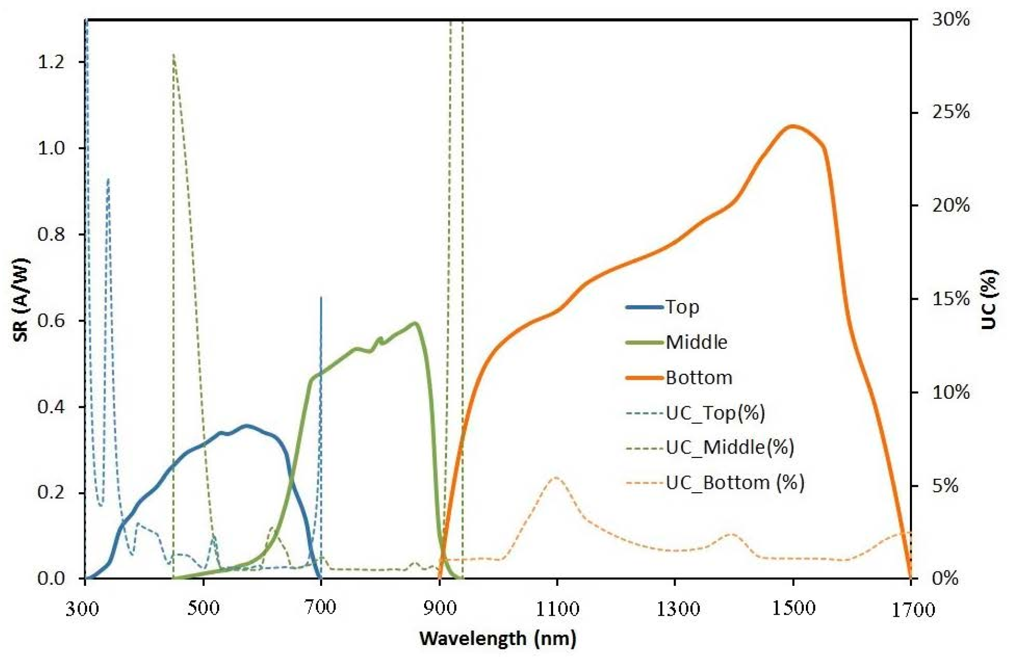
Figure 2.
Measured spectra and reference spectrum AM1.5D ed.3 with the uncertainty function. The spectrum acquired at 07:50 would lead to SMR values outside the 3% limit, due to the low content in the UV and the visible. However, it has been included in the analysis to check that the results are applicable to all the hours of the day, and not only close to AM1.5D conditions.

Figure 3.
Spectral matching ratios during the day, calculated using the measured spectra and spectral responses without any added error. The four triplets of spectral matching ratios (SMR) given by the spectra used in this study are highlighted.
Figure 3.
Spectral matching ratios during the day, calculated using the measured spectra and spectral responses without any added error. The four triplets of spectral matching ratios (SMR) given by the spectra used in this study are highlighted.
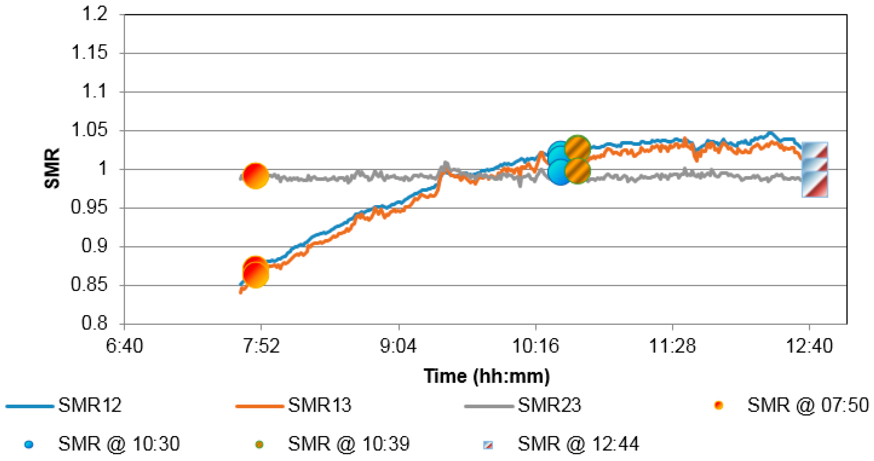
Figure 4.
Impact of the errors on top junction spectral responsivity on SMR12 and SMR13 (k = 1). The slope of the functions indicates how much the output error is sensitive to an accurate estimation of the input errors on the top junction spectral response.
Figure 4.
Impact of the errors on top junction spectral responsivity on SMR12 and SMR13 (k = 1). The slope of the functions indicates how much the output error is sensitive to an accurate estimation of the input errors on the top junction spectral response.

Figure 5.
Impact of the errors on Middle junction spectral responsivity on SMR12 and SMR23 (k = 1). The slope of the functions indicates how much the output error is sensitive to an accurate estimation of the input errors on the middle junction spectral response.
Figure 5.
Impact of the errors on Middle junction spectral responsivity on SMR12 and SMR23 (k = 1). The slope of the functions indicates how much the output error is sensitive to an accurate estimation of the input errors on the middle junction spectral response.

Figure 6.
Impact of the errors on Bottom junction spectral responsivity on SMR13 and SMR23 (k = 1). The slope of the functions indicates how much the output error is sensitive to an accurate estimation of the input errors on the bottom junction spectral response.
Figure 6.
Impact of the errors on Bottom junction spectral responsivity on SMR13 and SMR23 (k = 1). The slope of the functions indicates how much the output error is sensitive to an accurate estimation of the input errors on the bottom junction spectral response.

Figure 7.
Impact of random errors of measured spectrum on the three SMR. The linearity of the functions is notable, and the slopes indicate that the spectral random errors have the same impact on all the three SMR. (a) case of SMR12; (b) case of SMR13; (c) case of SMR23.
Figure 7.
Impact of random errors of measured spectrum on the three SMR. The linearity of the functions is notable, and the slopes indicate that the spectral random errors have the same impact on all the three SMR. (a) case of SMR12; (b) case of SMR13; (c) case of SMR23.

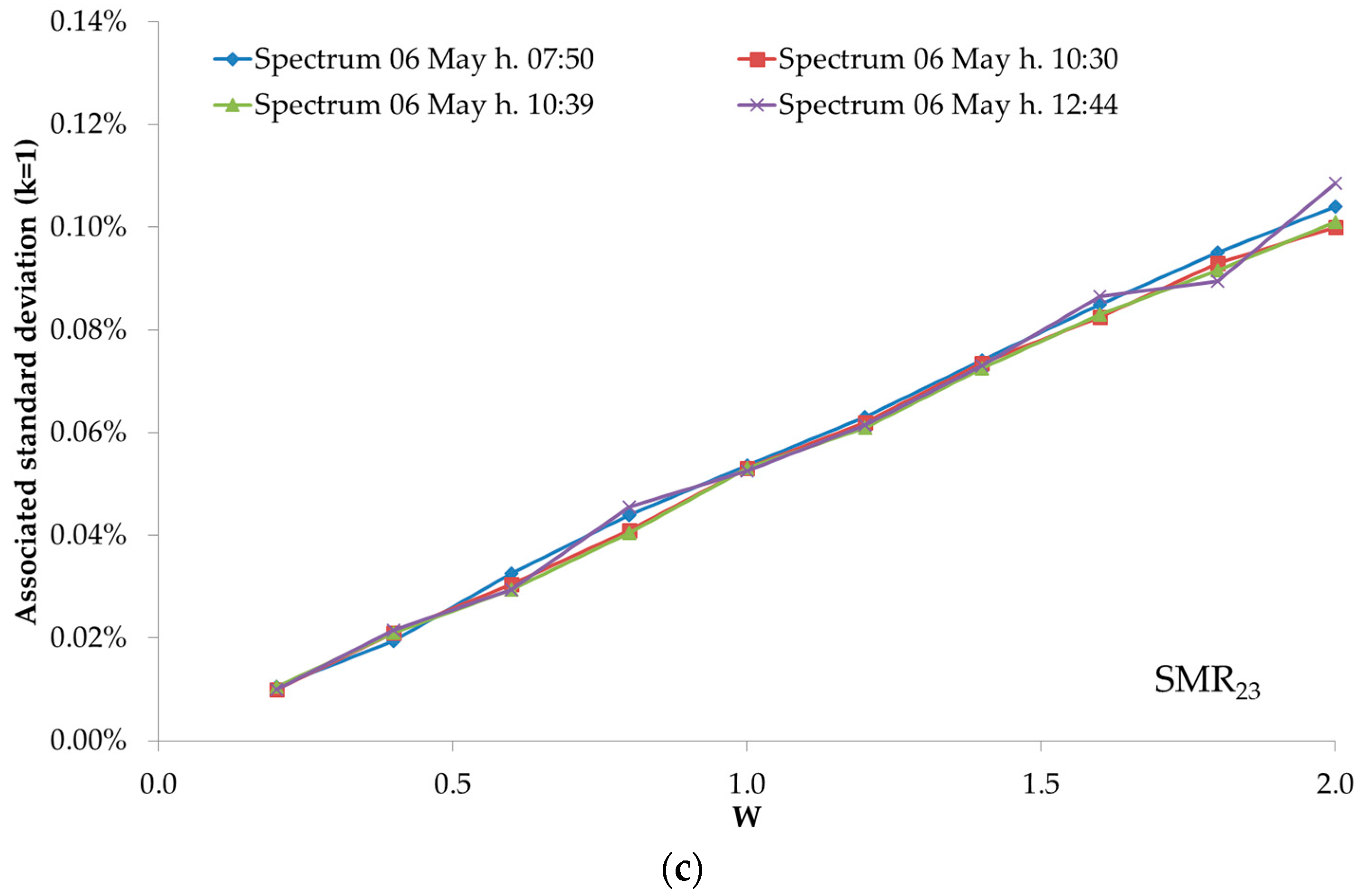
Figure 8.
Weighting factor generated in 3 different Monte Carlo runs to adjust the spectrum in the InGaAs and c-Si regions independently. The weighting factor is always equal to one except in the interested wavelengths, where the spectrum is scaled up or down depending on the random number sampled from the Gaussian distribution.

Figure 9.
Uncertainties associated with spectroradiometer c-Si and InGaAs temperature errors, varying the amplitude of the temperature error. (a) crystalline silicon detector in the region 850 ≤ λ ≤ 1150 nm; (b) InGaAs detector in the region 1500 ≤ λ ≤ 1700 nm.
Figure 9.
Uncertainties associated with spectroradiometer c-Si and InGaAs temperature errors, varying the amplitude of the temperature error. (a) crystalline silicon detector in the region 850 ≤ λ ≤ 1150 nm; (b) InGaAs detector in the region 1500 ≤ λ ≤ 1700 nm.


Table 1.
Variations associated with spectroradiometer temperature errors for the case input σ = ±1.5 °C.
Table 1.
Variations associated with spectroradiometer temperature errors for the case input σ = ±1.5 °C.
| () | σ (SMR12) | σ (SMR13) | σ (SMR23) |
|---|---|---|---|
| c-Si | 0.05% | 0.10% | 0.15% |
| InGaAs | 0 | 0.08% | 0.08% |
Table 2.
Variations associated with all the input uncertainties using a Monte Carlo approach compared with the squared sum of all the contributions. The “±” sign is omitted for clarity.
Table 2.
Variations associated with all the input uncertainties using a Monte Carlo approach compared with the squared sum of all the contributions. The “±” sign is omitted for clarity.
| (k = 1) | σ (SMR12) | σ (SMR13) | σ (SMR23) |
|---|---|---|---|
| Spectrum 07:50 | 0.10% | 0.15% | 0.21% |
| Spectrum 10:30 | 0.09% | 0.17% | 0.23% |
| Spectrum 10:39 | 0.08% | 0.14% | 0.17% |
| Spectrum 12:44 | 0.09% | 0.15% | 0.21% |
| Average | 0.09% | 0.15% | 0.21% |
| Expanded UC (k = 2) | 0.18% | 0.30% | 0.42% |
© 2018 by the authors. Licensee MDPI, Basel, Switzerland. This article is an open access article distributed under the terms and conditions of the Creative Commons Attribution (CC BY) license (http://creativecommons.org/licenses/by/4.0/).
Share and Cite
MDPI and ACS Style
Pavanello, D.; Galleano, R.; Kenny, R.P. Uncertainty Propagation of Spectral Matching Ratios Measured Using a Calibrated Spectroradiometer. Appl. Sci. 2018, 8, 186. https://doi.org/10.3390/app8020186
AMA Style
Pavanello D, Galleano R, Kenny RP. Uncertainty Propagation of Spectral Matching Ratios Measured Using a Calibrated Spectroradiometer. Applied Sciences. 2018; 8(2):186. https://doi.org/10.3390/app8020186
Chicago/Turabian StylePavanello, Diego, Roberto Galleano, and Robert P. Kenny. 2018. "Uncertainty Propagation of Spectral Matching Ratios Measured Using a Calibrated Spectroradiometer" Applied Sciences 8, no. 2: 186. https://doi.org/10.3390/app8020186
Note that from the first issue of 2016, this journal uses article numbers instead of page numbers. See further details here.