An Automatic Navigation System for Unmanned Surface Vehicles in Realistic Sea Environments


School of Marine Electrical Engineering, Dalian Maritime University, Dalian 116026, China
*
Author to whom correspondence should be addressed.
Appl. Sci. 2018, 8(2), 193; https://doi.org/10.3390/app8020193
Submission received: 30 December 2017
/
Revised: 17 January 2018
/
Accepted: 23 January 2018
/
Published: 28 January 2018
Abstract
:In recent years, unmanned surface vehicles (USVs) have received notable attention because of their many advantages in civilian and military applications. To improve the autonomy of USVs, this paper describes a complete automatic navigation system (ANS) with a path planning subsystem (PPS) and collision avoidance subsystem (CAS). The PPS based on the dynamic domain tunable fast marching square (DTFMS) method is able to build an environment model from a real electronic chart, where both static and dynamic obstacles are well represented. By adjusting the , the generated path can be changed according to the requirements for security and path length. Then it is used as a guidance trajectory for the CAS through a dynamic target point. In the CAS, according to finite control set model predictive control (FCS-MPC) theory, a collision avoidance control algorithm is developed to track trajectory and avoid collision based on a three-degree of freedom (DOF) planar motion model of USV. Its target point and security evaluation come from the planned path and environmental model of the PPS. Moreover, the prediction trajectory of the CAS can guide changes in the dynamic domain model of the vessel itself. Finally, the system has been tested and validated using the situations of three types of encounters in a realistic sea environment.
1. Introduction
In line with the growing interest in the ocean for civilian and military applications, there has been an increasing demand for the autonomy of unmanned surface vehicles (USVs) with advanced automatic navigation systems (ANSs) [1]. USVs are intelligent unmanned platforms which perform tasks independently in a variety of cluttered sea environments and have highly nonlinear dynamic characteristics [2]. The development of USVs has brought many advantages, such as improved personnel safety and reduced operation costs, as well as increased autonomy and flexibility in sophisticated environments [3,4]. However, now only semi-autonomous USVs are used rather than fully-autonomous USVs. This is due to the complex and hazardous sea environments [5]. The ANS in this paper is designed for fully-autonomous USVs in order to minimize both the need for human control and the effects due to human error. To ensure that a fully-autonomous USV travels in a realistic sea environment, the ANS is composed of a path planning subsystem (PPS) and a collision avoidance subsystem (CAS). The PPS can generate a shorter path according to the current environment in a collision-free and smooth manner. In the local environment, the CAS not only follows the reference path points, but also has the control capacity to avoid collision in a timely manner.
In terms of USVs, there are an increasing number of algorithms in the research focusing on path planning as a fundamental aspect of ANSs. These include Dijkstra’s algorithm [6], A* [7,8], Theta* [9], the Voronoi diagram [10], particle swarm optimization (PSO) [11], ant colony optimization (ACO) [12,13], the genetic algorithm (GA) [14], and so on. Recently, considering the turning capacity of USVs, Yang and Tseng used the finite Angle A* algorithm (FAA*), which is used to determine safer and suboptimal paths for USVs on satellite thermal images [7]. Kim put forward the angular rate-constrained Theta* algorithm with considerations of vehicle performance based on the Theta* algorithm [9]. However, all of these algorithms search the optimal path in a static environment. Hence, path re-planning (collision avoidance) is proposed to meet the demands of real-time planning or avoidance under dynamic environments. These algorithms include the rolling windows method [11], artificial potential field (APF) [6,12], velocity obstacle (VO) [15,16], local reactive obstacle avoidance [17], optimal reciprocal collision avoidance [18], dynamical virtual ship (DVS) [19], and so on. Although these algorithms have good real-time performance, they are difficult to use in complex and irregular environments. To solve this problem, some scholars use the hierarchical structure to combine global path planning and local path re-planning [6,11,12], and some try to improve the traditional path planning algorithm, using for example Rule-based Repairing A* [8]. Liu et al. selected the fast marching method (FMM)-based path planning algorithm [20]. The advantage of the FMM is that it is capable of fast generating optimal and smooth trajectories in a complex environment, which enables it to be applied in dynamic and static environments. Hence, the PPS of this paper is based on the FMM algorithm.
In addition, although many works in the literature (see e.g., [6,7,9]), use satellite maps for environmental information, this method is incomplete for describing the invisible sea environment, such as reefs, ocean depths, and so on. Thus in this paper, environmental information is obtained from the electronic chart, which can display this invisible information in detail.
After planning the path, according to the guidance, navigation, and control (GNC) system structure [1] the next step is to control the USV following the path. Some works have discussed this problem after generating the path. The authors of [10,20,21], for instance, employed the line-of-sight (LOS) guidance algorithm to convert the path following the course control of USVs. Zhang used a robust neural control algorithm to follow the path generated by the DVS [19]. Woo adopted a double-loop indirect track-keeping control structure with the Proportional-Integral-Derivative (PID) control algorithm [22]. Nevertheless, these studies focused solely on path-following or trajectory-tracking algorithms, and these algorithms assume the impossibility of collisions during the tracking process [5]. The failure or delay of the guidance system will cause the USV to lose the collision avoidance ability. In consequence, it is important for USVs to adopt the collision avoidance control algorithm in the CAS. To date, the collision avoidance control algorithm has been developed in mobile robots [23], unmanned vehicles [24,25], and unmanned aerial vehicles (UAVs) [26], but there are few studies on USVs. A CAS for USVs emerged in relevant literature [8], in which the fuzzy estimator method was developed for collision avoidance control. The method is able to avoid collision with a change of course. However, collision avoidance not only needs to change the course, but also the speed needs to be adjusted. Model predictive control (MPC), which combines path planning with on-line stability and convergence guarantees, is increasingly being applied to collision avoidance problem [27]. One significant study can be found in the work undertaken by Johansen [28], who applied MPC in the CAS of ship with a simple external environment. However in contrast to ordinary ships, considering that USVs have the characteristics of high speed and smaller volume, the CAS needs shorter computation times and stronger robustness. Finite control set model predictive control (FCS-MPC) is used as the collision avoidance control algorithm, and has advantages such as fast dynamic response, optimal control of multiple objectives, inherent decoupling, and easy inclusion of nonlinear constraints [29].
To improve the autonomy of USVs, an ANS with a PPS (dynamic domain tunable fast marching square, DTFMS) and CAS (FCS-MPC) is proposed in this paper. The main contributions of this paper can be summarized in five main points. Firstly, the proposed DTFMS method is able to construct a potential map from a real electronic chart, where both static and dynamic obstacles are well represented. To represent the dynamic obstacles, the algorithm adds the dynamic domain models of own and target vessels into the planning space, and the domain models can be changed according to vessel motion states and updated environment times. Secondly, the proportion of the safe area in potential maps can be adjusted by to assess security and path length. Thirdly, using the potential map from the DTFMS method, a collision-free smooth path can be generated which can be used as dynamic target points of the CAS. Fourthly, a fast and safe CAS is proposed based on FCS-MPC, and it has the ability for trajectory tracking and local collision avoidance for underactuating USVs. Meanwhile, to fully evaluate the safety of the predicted trajectories, its security evaluation comes from the potential map of the DTFMS method. Finally, the simulations are undertaken in a realistic sea environment with three types of encounter situations, and the target vessels have the possibility of changing their course, which is similar to the practical context.
The rest of the paper is organized as follows. Section 2 introduces the structure of the USV system. Section 3 describes the static environment modeling and path planning method. Section 4 establishes the mathematical model of the USV and designs the CAS based on FCS-MPC. In Section 5, the DTFMS method is proposed for path re-planning in a dynamic environment. In Section 6, the ANS is verified in the simulation and real environments, and their results are compared in the dynamic and static cases. Finally, Section 7 gives the conclusions on the system and identifies future works on the ANSs of USVs.
2. The Overview of Unmanned Surface Vehicle System
The overall structure of the USV system has been systematically described in Figure 1, which illustrates the system with its three major subsystems (the state awareness system, executive system, and autonomous navigation system (ANS)) and the information flow between them. In the paper, the Lanxin USV, which is a small intelligence equipment platform of Dalian Maritime University [30], is used as the research object. The USV is a pod propulsion vessel, so its executive system command is composed of thruster speed and propulsion angle. The environmental information is divided into static information and dynamic information. The static environmental information can be obtained by electronic charts or satellite images. The surrounding dynamic information mainly comes from state awareness systems through on-board equipment (global positioning system (GPS), radars, cameras, and sonar) and the sharing of information with other vessels using radio, automatic identification system (AIS), and network communication. The two kinds of information are applied to global path planning and local path re-planning, respectively.
As observed from the USV system structure, the autonomous navigation system plays an important role as it connects both the state awareness system and the execution system. It contains two components, i.e., the PPS and CAS. The PPS can model the static and dynamic environment and generate optimized reference path points by path planning and re-planning and provide them to the CAS. The CAS generates control commands to the executive system that enables the USV to follow the reference path points and complete the local dynamic obstacle avoidance. Meanwhile, the predicted movement information of the USV from the CAS can provide reference for path re-planning. Detailed descriptions of the ANS are given in Section 3, Section 4 and Section 5. In order to realize the autonomous navigation of the USV, we make following assumptions:
- The state information of the obstacle is known exactly.
- We have real-time detection of the USV’s position, heading, and velocity.
- Global information comes from the electronic chart.
- The mathematical model of the USV can be used to predict future trajectories to evaluate the effect of control commands.
The proposed structure implies that collision avoidance and control functionality are integrated together. This leads to a more concise structure whereby the controller can directly implement the collision avoidance function, and reliability and safety can be ensured by the structure.
3. The Static Environment Modeling and Path Planning
3.1. Simulation Environmental
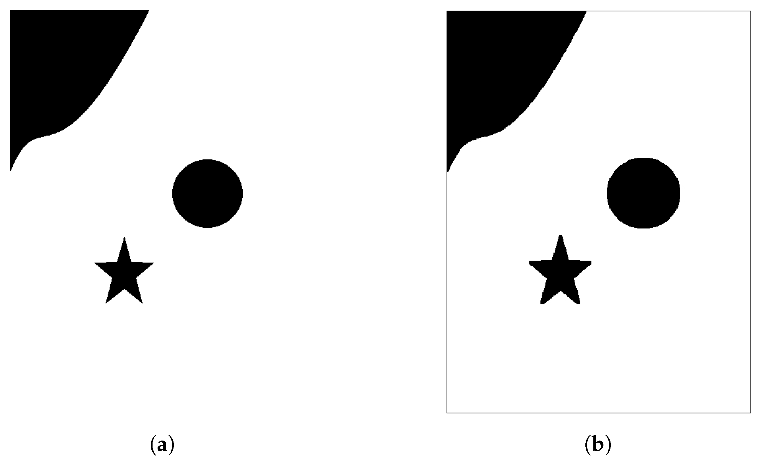
In Figure 2a, the simulation environment includes an irregular coastline and two islands (circular and pentagram), the dimension of which is 463 pixels × 613 pixels. Each pixel represents 1 m. According to the improved GoodWin ship domain model by Davis, when the obstacles are extended by a distance of half the ship’s length, the ship can be seen as a particle [31]. Hence, the simulation environment is extended by a distance of half the USV’s length, and added to the one-pixel-wide boundary in Figure 2b.
Moreover, the system removes all the height information in the environment, i.e., the three-dimensional (3D) environment is converted to a two-dimensional (2D) planar environment. According to the above hypothesis, USV can be seen as a particle motion in a 2D planar environment.
3.2. The Fast Marching Method
The FMM is a level set method proposed by Sethian in 1996 to solve the wave propagation problem [20]. It can also be used as a kind of the grid search algorithm in path planning with the continuity and smoothness of the path. This method can be divided into two steps. The first step is the exploration process, which establishes the optimal cost value (arrival time) of each grid on the whole map. The last step is the development process. That is, by solving the optimal cost value, the optimal path is formed from the target to the starting point. The exploration process is very similar to the expansion of waves. The path of waves from the source point to the target point can be considered as the optimal path, so we can establish the time function based on the propagation of waves. The FMM calculates the arrival time T for a wave to reach every point of the space. The wave can be generated by more than one source point, and each point originates one wave. The corresponding time of the source point is .
where is the time that the wave interface requires to reach , and is the source point.
When Equation (1) is a derivative of t, the inner product of two vectors about and speed V of wavefront can be obtained.
That is, at the point , the motion of the front is described by the Eikonal equation. The numerical solution of Equation (2) can be obtained via the upwind deferential method when using the FMM. The solving process of the FMM is similar to Dijkstra’s method but in a continuous way.
Suppose needs to be solved and its neighbor is a point set containing four elements , , , . The discretization of the gradient according to [32] derives to the following equation:
where
and and are the grid spacing in the x and y directions. Substituting (4) in (3) and letting
the Eikonal Equation can be rewritten for a discrete 2D space as:
Consequently Equation (6) can be solved as the following quadratic:
Assuming that the velocity is positive , T must be greater than and , that is, the front wave passes over the coordinates only once.
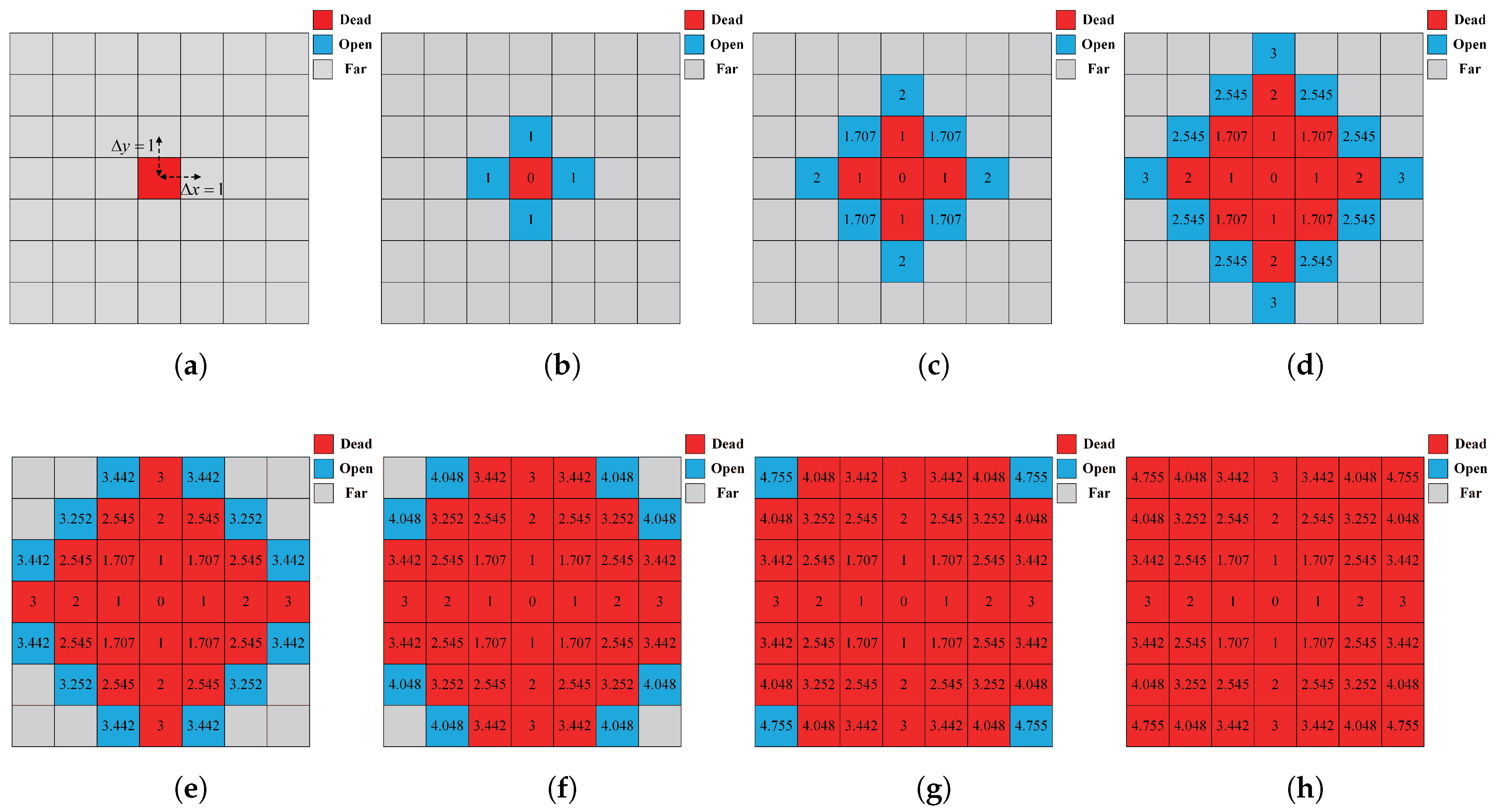
To further illustrate the FMM algorithm, a simple case representing how to update a grid map is shown in Figure 3. Figure 3a shows the initial configuration of the algorithm with the middle point being the algorithm start point. The interface propagating speed is set to be uniform as 1 at each grip point. When the FMM is being executed, grid points are categorized into three different groups as:
- Dead (marked as red): indicates that the arrival time value of the grid point has been calculated and determined;
- Open (marked as blue): indicates that the arrival time value of the grid point is an estimated value and may be changed;
- Far (marked as gray): indicates that the arrival time value of the grid point is unknown.
The arrival time output of one wave source in grid map is shown in Figure 4a. If we select T as the z axis of the third dimension, the result of the wave expansion is shown in Figure 4b. In the case of the four wave sources expanding, the same process is applicable. When the waves from different sources reach each other, the propagation continues as if they were only one wave, as shown in Figure 4c,d. With one single source, there is only one minima at the source. For more than one source, there is a minima at each source with .
Suppose Figure 2b, which is a binary map, represents the planning space . Its arrival time matrix T (shown in Figure 5a) from the end point is calculated by FMM. Then, on the base of the T, by applying the gradient descent method the optimal path is finally generated and shown as the magenta line in Figure 5b,c.
3.3. The Tunable Fast Marching Square Method
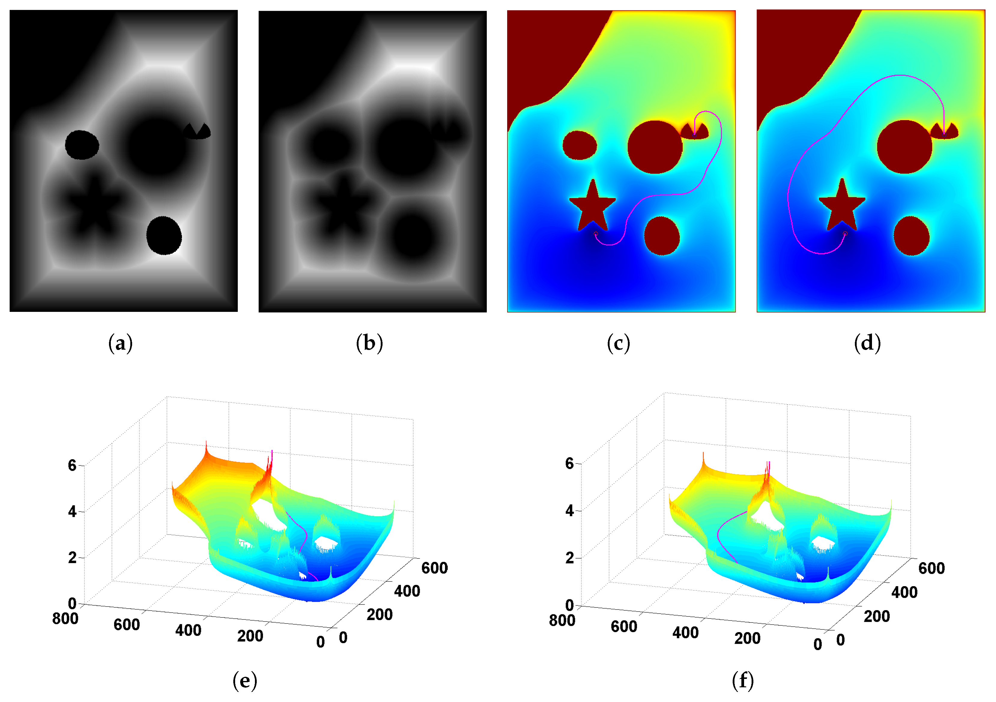
In the Figure 5, the path generated by FMM is too close to obstacles. In the real sea environment, there are usually shallow water near the islands and coastlines. This is dangerous for USVs. Hence, USVs should be as far away from obstacles as possible for safety. The literature [33] has proposed a new algorithm named the fast marching square (FMS) method to tackle this problem, which adds one step to the conventional FMM algorithm. First, the FMS method generates a security potential map with the FMM executing from all the points in obstacle area (see Figure 6a) by using the previous planning space. Its specific principle is multiple wave source expansion of the FMM, as shown in Figure 4c,d. The potential map V is the arrival time matrix of the wave. Then, with the potential map V as the speed matrix, the FMM is again applied to generate the arrival time matrix T from the end point in Figure 6b. The final path generated by the FMS method is shown as the magenta trajectory in Figure 6c,d with increased safety.
However, the path generated by FMS method is the farthest route from the obstacles, i.e., in the safest area. The farther away from the obstacles, the longer the length of the path. Hence, the tunable fast marching square (TFMS) method is proposed to tradeoff between security and path length. This method only changes the potential map of the FMS method. The TFMS method needs to scale the V into the range of 0 to 1 and , where is the scaled potential map and describes security from 0 to 1, and then rescales the V into range of 0 to 1. Figure 7 shows the result of path planning with different values in the potential map of the TFMS method. The TFMS is FMS when is 1.0, and FMM when is 0.0.
3.4. The Realistic Sea Environment Model
A sea area in Dalian harbor, which as a non-freezing deep-water harbor is one of the busiest harbors in China, was selected as the sea environment modeling area. Its electronic chart and binary map are shown in Figure 8a,b. The coastlines and ocean depth are clearly marked in the electronic chart, so it is clear that both collision area and safe area can be identified. In the electronic chart, the pixel values of the collision area are replaced by 0. The collision area is shown as black. The safe areas are replaced by the value 1 shown in white. The final map is the binary map that has only two possible values (0 or 1) for each pixel. The dimensions of the binary map are 1253 × 1794 pixels with the 1 pixel = 1 m scale. The results from applying the steps of TFMS method with 0.9 are shown in Figure 8c–f for the real sea area.
4. Collision Avoidance System
4.1. Finite Control Set Model Predictive Control of the CAS
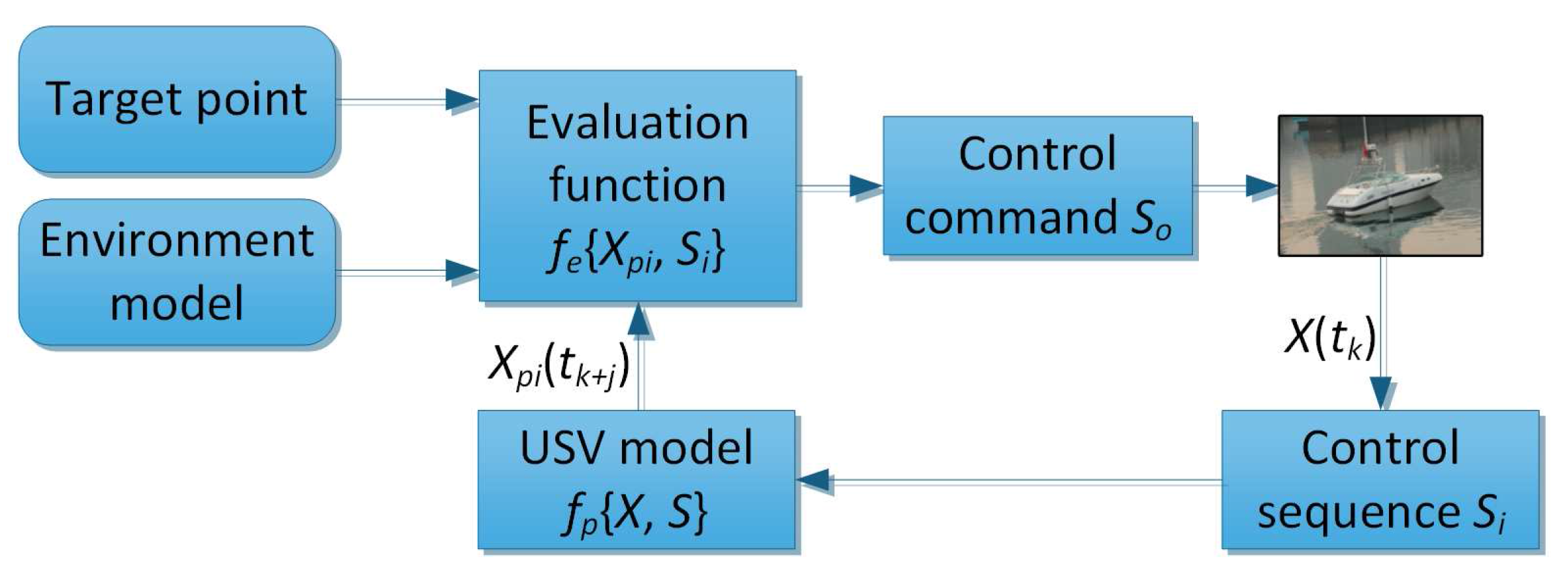
Based on the USV model, the FCS-MPC for the CAS predicts the possible trajectories by the finite control behaviors (finite control set), and then judges all these trajectories by the predefined evaluation function to select an optimal control behavior. Figure 9 illustrates a block diagram of the FCS-MPC for the CAS.
The design process of the system is as follows: The USV prediction model first needs to be established, and can predict the USV’s state quantity X in response to the different control behaviors S. At time , by the USV prediction model, the predictive values of the state quantity under the action of can be calculated based on the current state quantity , i.e., , . c is the number of all valid control behaviors of USV, , and is prediction horizon. Based on the system characteristics concerned, such as attainability, safety, stability, and rapidity, the evaluation function is constructed. Finally, the selected control command that makes the function optimal is used to control the USV.
4.2. Prediction Model of USV
The prediction model of the USV is described by the standard three-degree of freedom (DOF) planar ship motion model, neglecting the roll, pitch and heave motions [34]. The kinematics of the system can be written as
where represents position and course in the earth-fixed frame, includes surge and sway velocities and yaw rate in the body-fixed frame, and is rotation matrix from body-fixed to earth-fixed frame. The and together form the state quantity X of USV, which is
Assume that:
- The environment force can be neglected in the model;
- The inertia, added mass, and damping matrices are diagonal.
The simplified model of vessel can be written as [35,36]
with [37,38]
where values are given by the vessel inertia and the added mass effects, values are given by the hydrodynamic damping, L is the USV length, T is thrust of thruster, and the inputs of model are the propulsion angle and thruster speed n.
Based on the servo response characteristics of the actual steering process and the actual data collected from the experimental process, the steering gear response model is processed according to the second-order link [37,39]
Here, is the command propulsion angle, and , , and K represent the natural frequency, damping ratio, and proportionality coefficient, respectively. is the actual propulsion angle range.
4.3. Control Behaviors and Prediction of the USV Trajectory
For the USV system, the control behavior S is the combination of propulsion angle (which replaces the command propulsion angle later) and thruster speed n. The actuator of the USV has a lot of limitations, such as maximum value and , change rate , and the of the two control behaviors. In the control update interval , the scope of the control behaviors is
and
Then, by the discrete propulsion angle and thruster speed , the maximum number of control behaviors is . With the decrease of and , the control behaviors will be more precise, which can improve the performance of the system, but the calculation complexity will increase accordingly. In terms of the control performance and safety, it is obvious that there should be as many control behaviors as possible, but from an information processing perspective, the calculation complexity should be reduced within the computational capacity. Obviously, there is a tradeoff between the number of the control behaviors and the computational complexity with respect to time discretization, the control update interval, the prediction horizon, and the computation time. In addition, a very useful feature of these control behaviors is that they should remain constant throughout the prediction horizon.
4.4. Evaluation Function
To ensure the CAS meets some requirements, such as attainability, safety, stability and rapidity, the system proposes the evaluation function , including four subfunctions i.e., , , , and corresponding to the four demands, respectively. The normalization method is used to smooth the evaluation function. For instance, the normalized first subfunction is
Moreover, according to the importance of these demands, evaluation subfunctions can have different weightings . The ith evaluation function is
We set the control behavior that can maximize the evaluation function as the optimal control command. The four subfunctions are defined as follows.
4.4.1. Attainability Subfunction
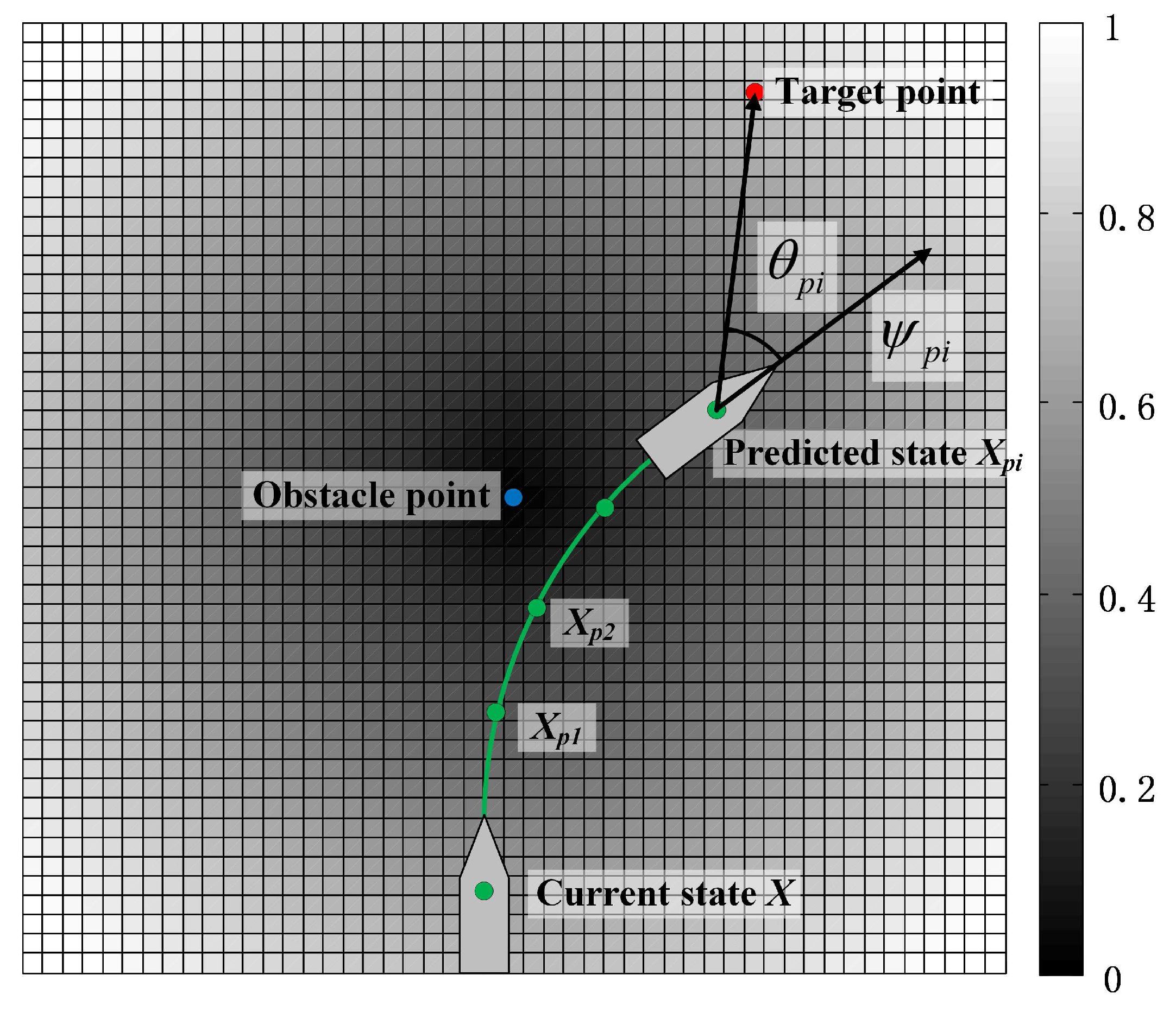
The first demand of the CAS is to reach the target point. If the course keeps pointing to the target point, which is called the navigation angle, the vessel can reach the target point along the shortest path. Hence, the difference angle between the predicted course and the navigation angle can be used to evaluate the attainability of , as shown in Figure 10.
The attainability subfunction is
4.4.2. Safety Subfunction
The safety of the CAS is extremely important for the USV. The safety subfunction should ensure that the vessel is away from all obstacles in the surrounding environment. In Section 3, the value of potential map V, which is generated by the TFMS method, can describe the security of each pixel point from 0 to 1. Hence, the sum of the potential values corresponding to all the predicted states on ith trajectory is the safety evaluation of the trajectory. The safety subfunction is
where n is the number of states on ith trajectory. Figure 10 explains the safety subfunction in a potential map V with one obstacle point.
4.4.3. Stability Subfunction
In order to enable the USV to be as stable as possible, the propulsion angle should be smaller or zero. Thus, the stability subfunction is
4.4.4. Rapidity Subfunction
The rapidity of the USV can be described by its speed U as
4.5. Stop Distance and Hazard
According to the USV dynamics, stop distance also needs to be considered. The stop distance varies with the current state of the USV, that is, at the current speed, as much as possible to reduce the speed, the distances generated in this process are calculated by
where U and are the speed and acceleration of USV. When the stop distance is larger than the minimum distance between the vessel and the z obstacle points in a search range of radius , the ith control behavior is ineffective. The minimum distance is
where the represent the the state quantity of the kth obstacle point. If is replaced with X, the is hazard value of current state X.
4.6. Dynamic Target
For the above four subfunctions, we can adjust their weights according to their importance. The system selects the optimal control command in the range that the predicted trajectory can cover. However, when there is a concave obstacle, the algorithm can easily to fall into the local optimum, as shown in Figure 11. A dynamic target method is introduced to solve the problem.
Considering that the path planning system can generate the global optimal path point, if its path point closest to the prediction range is selected as a dynamic target (DT), the USV can be far away from the local optimal area, as verified in Section 6. Because the path planning process requires a certain computation time which results in an information updating delay, the update time should be considered. The distance of DT on the optimal path is
Using this method, the USV can not only follow the global optimal path point, but also have the local collision avoidance functionality.
5. Dynamic Environment Modeling and Path Re-Planning
In the dynamic environment, there are dynamic obstacles to the vessel itself, which can affect the optimal path generated. Hence, a method named the dynamic domain tunable fast marching square (DTFMS) method is proposed to establish the domain model for the own vessel and target vessel. The own vessel can makes collision avoidance actions and the target vessel does not take any collision avoidance actions.
5.1. The Dynamic Domain Tunable Fast Marching Square Method
5.1.1. Own Vessel Dynamic Domain Model
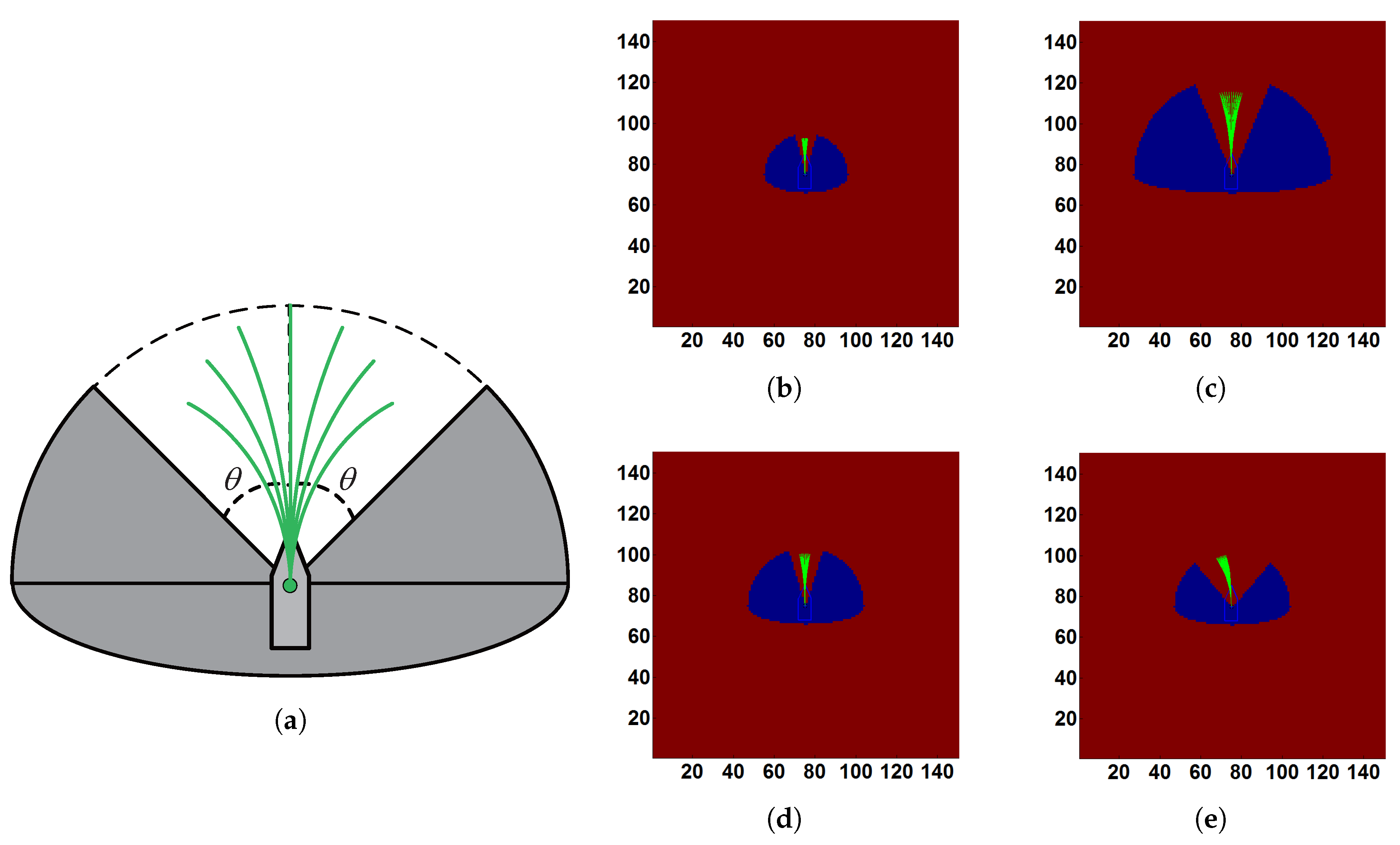
Even though the trajectory provided by the TFMS method is smooth and safe, motion characteristics of the USV are ignored, which causes the trajectory to have a lesser role in navigation. The USV is a kind of underactuated vehicle, so its surrounding area can be divided into reachable and unreachable areas. In the previous literature [20], the domain of the vessel itself was only considered as fixed, and ignored the dynamic movement of the USV. Thus, the DTFMS method is used to solve this problem based on the TFMS and FCS-MPC. Because the FCS-MPC can continuously update the reachable set of the vessel, when the control commands are updated, a series of vessel trajectories can be predicted, as the green lines show in Figure 12. In order to achieve a shape of reachable set that is easy to calculate in environment model, Figure 12a shows the dynamic domain model of the own vessel. It is composed of two parts,: the bow part is a semi-circle and the stern part is a semi-ellipse. The domain model changes its shape according to the speed U of the vessel; the shape tends to be circular when vessel is traveling at low speeds and semi-circular at high speeds. So that the domain contains a reachable set with update time , the radius of the bow part is the farthest distance from the predicted position to the current position, and the semi-major axis of stern is same as the radius of the bow.
The and are
with
where is minimum radius of domain model, which can be calculated by the length L of USV and safe distance . The domain model is divided into two (reachable and unreachable) areas. In Figure 12a, the reachable area is the white sector, including angles which are determined by the current course , predicted course , and minimum angle , that is
The own vessel domain can change dynamically with the speed and reachable set from the FCS-MPC. Figure 12b–e shows the own vessel domain with different speeds and included angles in the updated time = 4 s. In Figure 12b–d, the initial propulsion angle of the vessel is , but the angle is in Figure 12e, which better shows the relationship between the predicted trajectories of the FCS-MPC and included angles of the own vessel dynamic domain model.
5.1.2. Target Vessel Dynamic Domain Model
In the field of autonomous navigation, the concept of ship domain is often introduced, which is the area around the target vessel that prevents other moving objects from entering. The shape of the ship domain is usually circular, and its center is located at the instantaneous position of the target [31]. However, when the target vessel speed is high, the collision risk of bow direction is greater than in the abeam and stern directions. Hence, it is reasonable to build the ship domain according to the speed of the target vessel. Referring to ship domain of Tam [40], the domain model of the target vessel can be established in Figure 13a, and also changed by the two parameters and . They are given by
with
Referring to Figure 14, and are equal at low speed (until the speed reaches ); at high speed, gradually reduces to , while increases in proportion to U, as more emphasis is placed on the direction of travel of the target vessel at high speeds.
In Figure 13b–f, the domain model of the target vessel changes its shape according to the different speeds. The shape tends to be circular when vessel is traveling at low speeds so that the collision risks are equally allocated near the vessel. However, at high speeds the bow part is more at-risk than the other parts, and this part increases proportionally with speed.
5.2. The Process of Path Re-Planning
The process of path re-planning with the DTFMS method is described in Figure 15. First, the dynamic domain models need to be added to the potential map V. For example, Figure 15a adds one own vessel and two target vessels, and each addition time is of 0.08 s. The updated V is acquired by the TFMS method within 0.20 s in Figure 15b. Then the arrival time matrix T and path are generated within 0.20 s, as shown in Figure 15c,e. Figure 15d,f shows the impact of removing a target vessel on the path. As we can see, the path is updated according to the changes of the environment. Affected by the domain model, the new path can follow the current course and stay away from target vessels. Similarly, an actual environment example of path re-planning using the DTFMS method is shown in Figure 16.
In terms of computation time, the simulation environment (463 pixels × 613 pixels) by the DTFMS method requires 0.50 s to explore the space, whereas the realistic environment takes 3.80 s with dimensions of 1253 × 1794 pixels. Because the realistic environment needs to explore more space, it takes more time. Therefore, the update time we choose should be longer than the computation time of the algorithm.
6. Simulation Study and Discussion
The section discusses and analyses the proposed ANS of the with the DTFMS and FCS-MPC in two different environments. The first simulation is to validate the algorithm in a simulation environment, and two different test scenarios are designed: (1) the USV runs in a static environment; and (2) the USV operates in a dynamic obstacle environment. The second simulation is designed to test the algorithm in a realistic sea environment with static and dynamic environments. The modeling of the simulation and real environments has been described in Section 3 and Section 5. The parameters of the USV and the algorithm from Table 1 is used in all cases.
The algorithm is coded in Matlab and simulations are run on the computer with a Core i7 3.6 GHz processor and 4 GB of RAM. The simulation results are given by time-dependent motion sequences. The following symbols and color codes in motion sequence diagram are applied:
- The start and end points for the USV are marked as blue and red ‘∗’ markers. The end point can be enlarged to a red circular area, and if the USV enters the area, it can be considered to be finished. Moreover, the dynamic target is marked as yellow ‘∗’ marker.
- There are three curves of the USV in the diagram. The magenta curve is the planned path of the DTFMS method for the USV. The blue curve represents the track of the USV up to a final time. The green curves denote the predicted trajectories at the present time. The symbol of the USV is the blue boat form.
- To make the vessels easy to observe, the symbols of both the USV and the target vessels (TVs) are enlarged 15 times in terms of size.
- The curves and boat forms with red, orange, and cyan colors represent the tracks and symbols of TV1, TV2, and TV3, respectively.
6.1. Verification in Simulation Environment with Single Moving Target Vessel
In the first test, the simulation environment is static without any dynamic obstacles. The final result of the simulation is shown in Figure 17, which is depicted in both a binary map and the corresponding potential map. It is clear that both the collision area (in black) and safe area (in white) have been identified. We can see that the USV can travel smoothly and safely into the end area.
Then, in order to test the capability of the algorithm to avoid dynamic obstacles, the moving TV1, which has a similar size (7.00, 3.00) m and speed 10 m/s (19.4 kn) to the USV, is added into the simulation environment. Generally, there are three types of situations in which the two vessels encounter each other: overtaking, head-on, and crossing situations. The most dangerous situation is the head-on situation. So, on the premise of removing the motion information of the USV, the path of the target vessel given by the TFMS method reaches a head-on situation with the USV. The simulated target vessel may be hostile or have detection system failure. The simulation results recording the movement sequences of the vessels are represented in Figure 18. Figure 18a–c shows how the USV adjusts the course to the end point. As the initial course of the USV is opposite to the direction of the end point, the planned path of DTFMS method extends a certain distance to the direction of the course. Figure 18d–f illustrates how the USV avoids TV1. The two vessels form a head-on situation and starboard side turning is adopted by the USV in Figure 18d. After 43 s, the USV decelerates gradually and enters the end area in a safe state (Figure 18g,h). In the corresponding safety potential maps, it can be observed that the USV can stay well outside collision area (including static obstacles and the target vessel domain), which proves that the ANS is able to guarantee collision-free navigation of the USV. Figure 18h shows the comparison of the tracks in the dynamic environmental (blue solid curve) and the static environment (blue dashed curve).
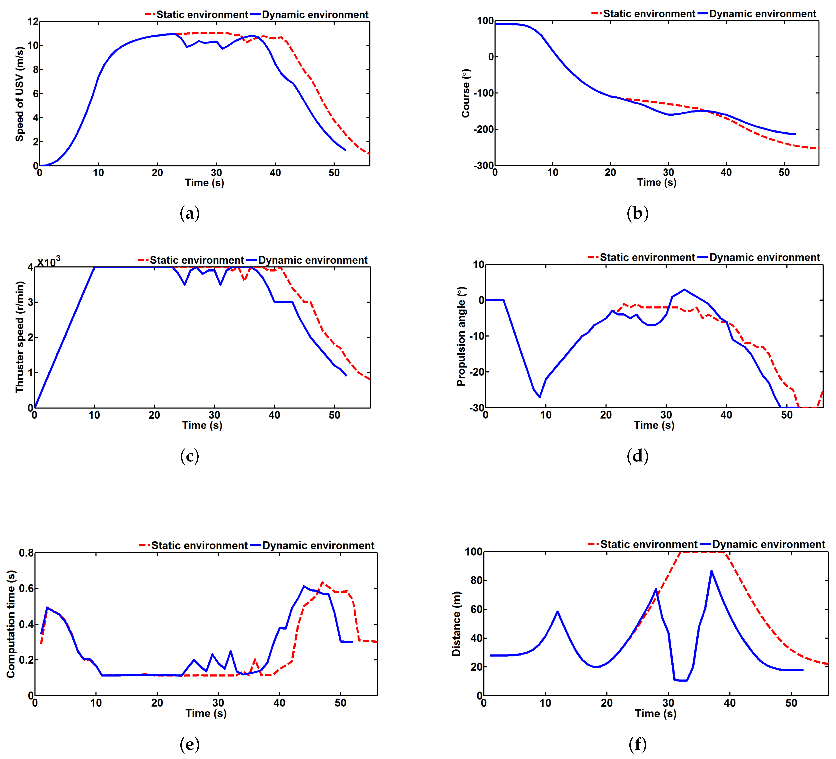
Evaluations of the USV behavior and algorithm performance in the dynamic and static environments are given in Table 2 and Figure 19. Table 2 describes the results of evaluation index of two tests. Figure 19a–d shows the control behaviors (thruster speed and command propulsion angle) and state output (speed and course) of the USV during the whole process. In Figure 19a,c, the USV and thruster keep at maximum speed during the sailing time, except for a slight decline in collision avoidance, which illustrates that the algorithm can adjust the speed according to the hazard under the premise of rapidity. In Figure 19d, at the beginning and the end of process, it is necessary to adjust the course with the larger command propulsion angle so that the USV can reach the end point. During the sailing time, the size of command propulsion angle is small at less than in a static environment, and less than in a dynamic environment, so the system also satisfies the stability. The update environment time is determined by the computation time of the system, which is divided into two parts, i.e., DTFMS method time 0.40 s and the FCS-MPC time. Figure 19e shows the computation time of the FCS-MPC. As a result of the maximum computation time of 0.63 s of the FCS-MPC, the is set to 2.00 s. Safety is the most important measure for autonomous navigation and should be ensured during the whole process. Figure 19f shows the distance between the USV and the detected collision area (the static obstacles after expansion and the target vessel domain). It can be seen that collisions will be detected at a longer distance in the two tests. The minimum and average distances are 19.8 m and 51.1 m in the static environment, and 10.4 m and 35.9 m in the dynamic environment, respectively.
6.2. Verification in Realistic Sea Environment with Multiple Moving Target Vessels
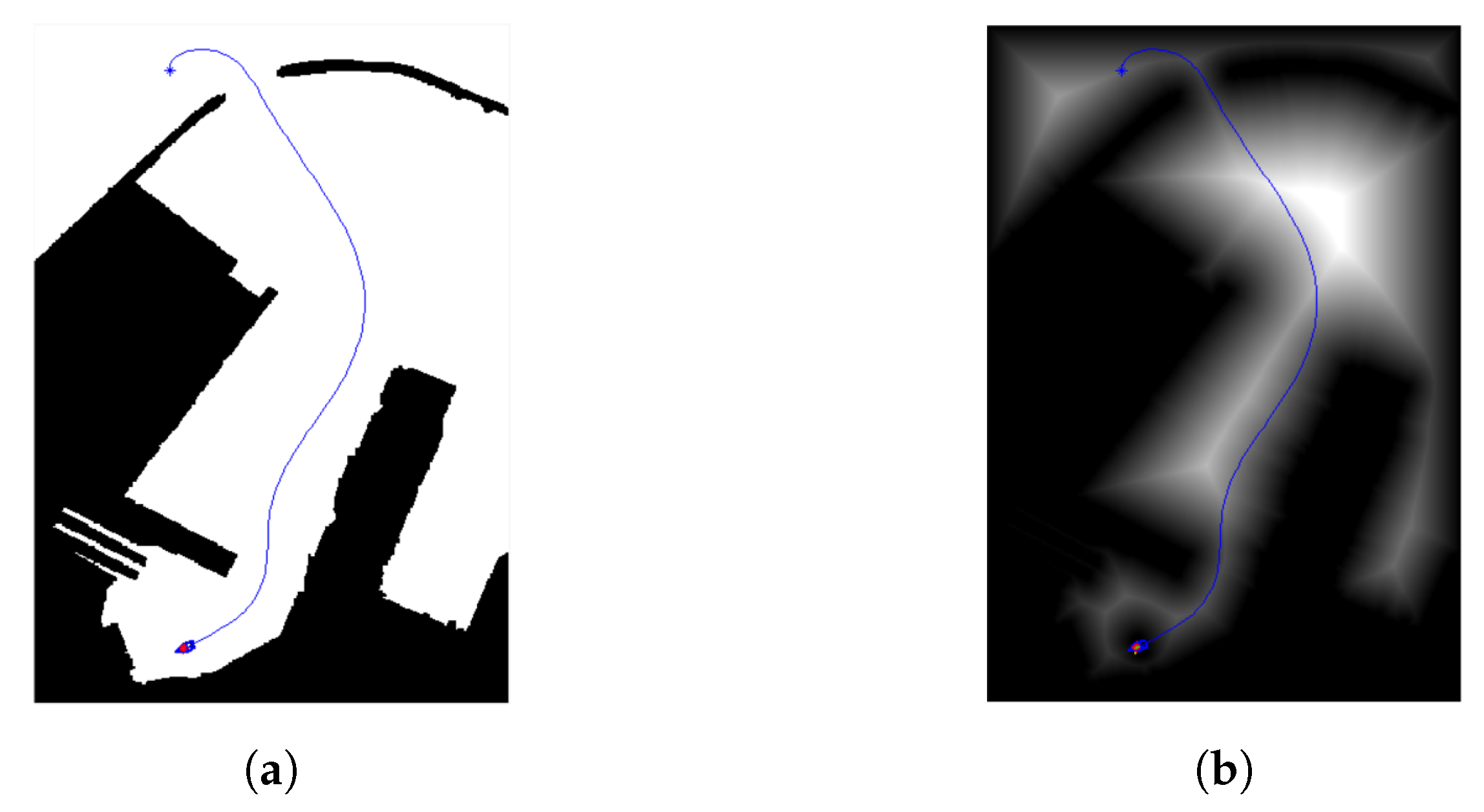
A more complex simulation is done in a realistic sea environment (shown in Figure 8a) with multiple moving TVs. Under the same algorithm parameter conditions, the USV first starts to sail in the static sea area and the final result is shown in Figure 20. It can be seen that the USV travels into the harbor in the safe area and eventually reaches the end area.
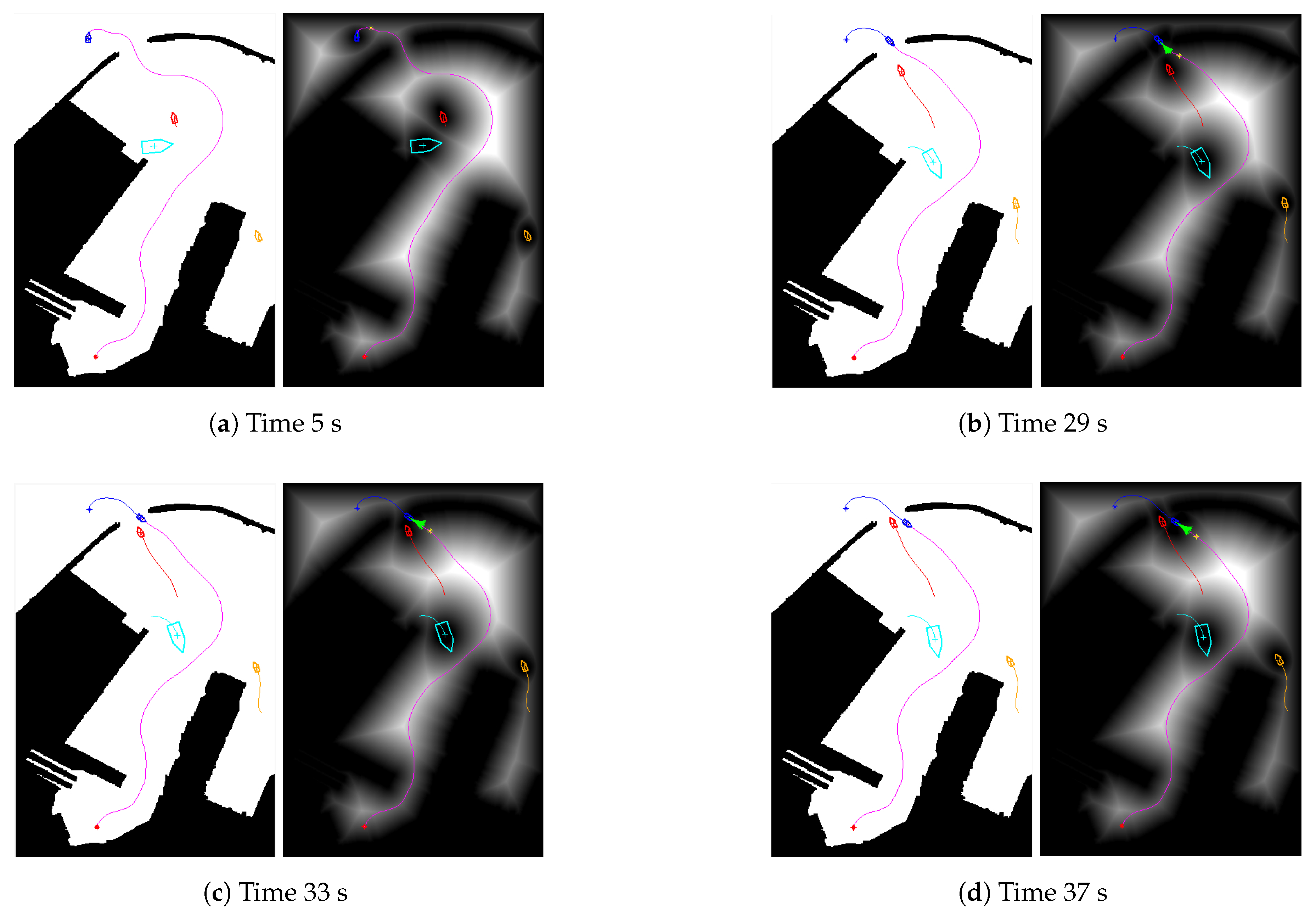
Now, three virtual TVs are added into the environment, traveling at 10 m/s (TV1), 7 m/s (TV2), and 5 m/s (TV3) respectively. The size (7.00, 3.00) m of TV1 and TV2 is similar to the USV, and TV3 measures (20.00, 8.00) m. In the same way, their path is also generated by the TFMS method without regard for other vessels. The movement sequences are expressed in Figure 21, which includes both the original binary maps as well as the potential maps. The potential maps show the vessel domain of three TVs based on their velocities. In addition, the system is verified in three encounter situations. Figure 21a,b plots the USV moving from the initial state to the harbor. At the entrance of the harbor, the USV encounters TV1 and forms a head-on situation. Next, Figure 21b–d displays the USV evasion process. After moving away from TV1, a crossing situation is made up of USV and TV2 in Figure 21e–g. When TV1 and TV2 are successfully avoided, the USV begins to overtake TV3. From Figure 21h–j, it is observed that the USV completed the task of overtaking, although TV3 changes its course in the process. The process of entering the end area is depicted in Figure 21k,l. Figure 21l shows the contrast of the final tracks of the USV in the two tests.
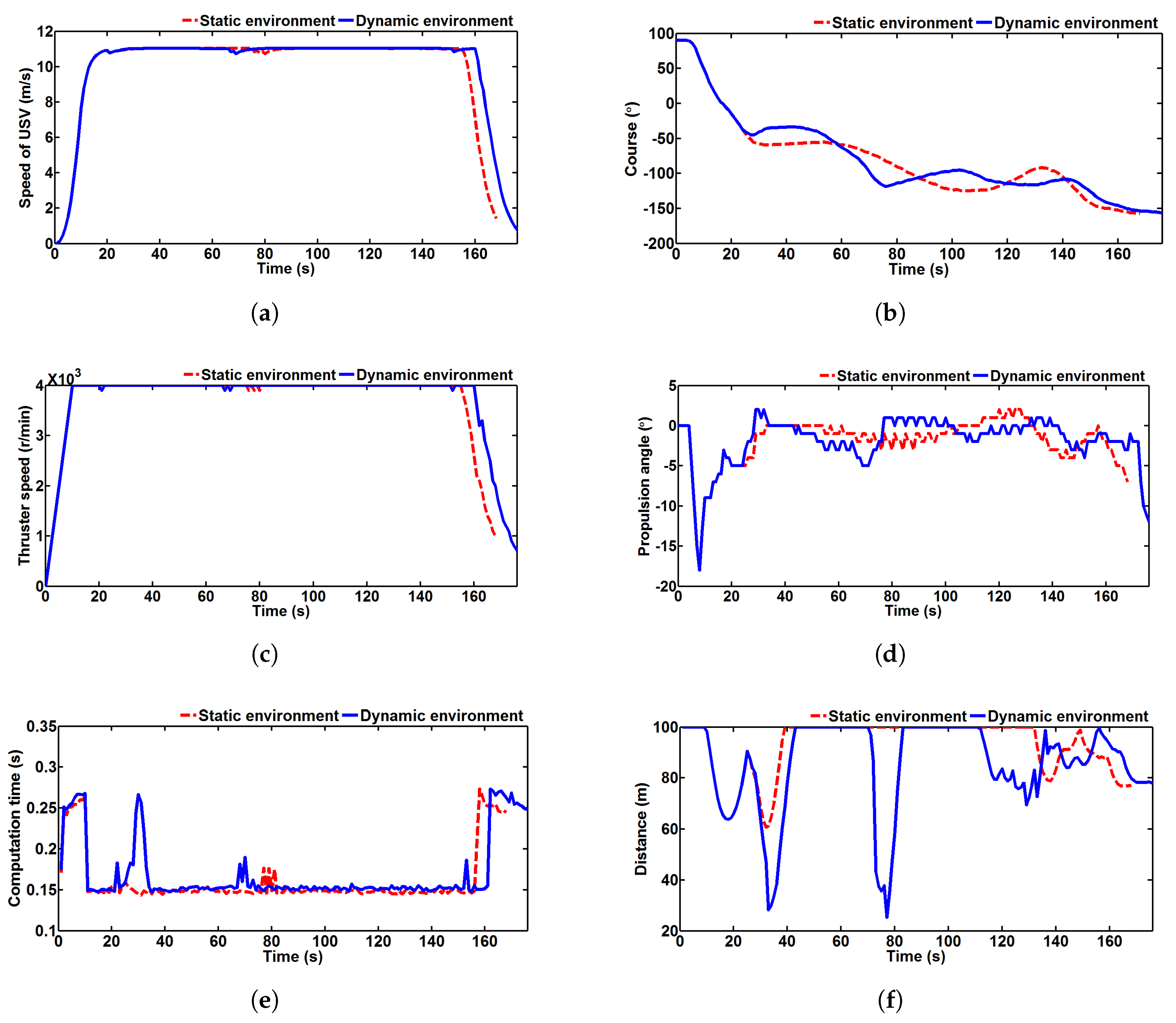
To assess the algorithm, first of all, in static and dynamic environments, the output and input of the USV are shown in Figure 22a–d and Table 3. In Table 3, the evaluation results of two tests is almost the same except for distance. Compared to the two tests, the speeds of the USV and thruster are largely the same and can maintain a maximum during the sail time in Figure 22a,c. In Figure 22d, the propulsion angle is completely consistent before collision avoidance. During the collision avoidance, the size of command propulsion angle is less than , similar to the static environment at less than . Figure 22e displays the computation time of the FCS-MPC. In the real environment, the DTFMS method time is 3.6 s which is far longer than the FCS-MPC time. The is selected as 4.00 s. Figure 22f records the distance between the USV and the detected collision area in the two tests. During the collision avoidance, the minimum distances of three situations are respectively 28.2 m, 25.4 m, and 69.3 m, which means that the USV is safe enough to drive.
7. Conclusions
In this paper, a complete ANS is presented with PPS (DTFMS) and CAS (FCS-MPC) in a realistic sea environment. First, the TFMS method is proposed to model the static sea environment and path plan, which can be adjusted by to weigh security and path length. Then, according to FCS-MPC theory, a CAS is developed to track trajectory and avoid collision based on a prediction model of the USV. The dynamic target point and security evaluation come from path planning and an environmental model of the PPS. Next, the proposed DTFMS method with dynamic domain models (a path re-planning algorithm), is able to well represent the dynamic vessels including the own and target vessels. There, dynamic domain models are changed according to the state of motion of the vessels and the environment update time. Finally, by comparing the static and dynamic tests, the simulation results validated the effectiveness of the proposed ANS in simulated and realistic sea environments.
Future work will firstly consider the problem that the practicability of ANSs can be further increased for real fully-autonomous USV experiments. First, to model a more real sea environment, the sea environment model needs additional altitudes and surface currents. Second, the collision avoidance control algorithm also needs to consider the problem of energy consumption and environmental influences (wind, waves and current). Thirdly, the Convention on the International Regulations for Preventing Collisions at Sea (COLREGs) should be considered in ANSs.
Acknowledgments
This work was partially supported by “the Nature Science Foundation of China” (Grant Number 51609033), “the Nature Science Foundation of Liaoning Province of China” (Grant Number 2015020022) and “the Fundamental Research Funds for the Central Universities” (Grant numbers 3132014321, 3132016312 and 3132017133).
Author Contributions
The work presented here was completed through the collaboration of all authors. Xiaojie Sun designed, analyzed, and wrote the paper. Guofeng Wang guided the full text. Yunsheng Fan conceived the idea. Dongdong Mu and Bingbing Qiu analyzed the data. All authors approved the manuscript.
Conflicts of Interest
The authors declare no conflict of interest.
References
- Liu, Z.; Zhang, Y.; Yu, X.; Yuan, C. Unmanned surface vehicles: An overview of developments and challenges. Ann. Rev. Control 2016, 41, 71–93. [Google Scholar] [CrossRef]
- Breivik, M. Topics in Guided Motion Control of Marine Vehicles. Ph.D. Thesis, Norwegian University of Science and Technology, Trondheim, Norway, 2010. [Google Scholar]
- Bertram, V. Unmanned Surface Vehicles—A Survey; Skibsteknisk Selskab: Copenhagen, Denmark, 2008; pp. 1–4. [Google Scholar]
- Breivik, M.; Hovstein, V.E.; Fossen, T.I. Straight-Line Target Tracking for Unmanned Surface Vehicles. Model. Identif. Control 2008, 29, 131–149. [Google Scholar] [CrossRef]
- Campbell, S.; Naeem, W.; Irwin, G.W. A review on improving the autonomy of unmanned surface vehicles through intelligent collision avoidance manoeuvres. Ann. Rev. Control 2012, 36, 267–283. [Google Scholar] [CrossRef] [Green Version]
- Xie, S.R.; Wu, P.; Liu, H.L.; Yan, P.; Li, X.M.; Luo, J.; Li, Q.M. A novel method of unmanned surface vehicle autonomous cruise. Ind. Robot Int. J. 2016, 43, 121–130. [Google Scholar] [CrossRef]
- Yang, J.M.; Tseng, C.M.; Tseng, P.S. Path planning on satellite images for unmanned surface vehicles. Int. J. Naval Archit. Ocean Eng. 2015, 7, 87–99. [Google Scholar] [CrossRef]
- Campbell, S.; Abu-Tair, M.; Naeem, W. An automatic COLREGs-compliant obstacle avoidance system for an unmanned surface vehicle. Proc. Inst. Mech. Eng. Part M J. Eng. Marit. Environ. 2014, 228, 108–121. [Google Scholar] [CrossRef]
- Kim, H.; Kim, D.; Shin, J.U.; Kim, H.; Myung, H. Angular rate-constrained path planning algorithm for unmanned surface vehicles. Ocean Eng. 2014, 84, 37–44. [Google Scholar] [CrossRef]
- Candeloro, M.; Lekkas, A.M.; Sorensen, A.J. A Voronoi-diagram-based dynamic path-planning system for underactuated marine vessels. Control Eng. Pract. 2017, 61, 41–54. [Google Scholar] [CrossRef]
- Wang, C.; Mao, Y.S.; Du, K.J.; Hu, B.Q.; Song, L.F. Simulation on Local Obstacle Avoidance Algorithm for Unmanned Surface Vehicle. Int. J. Simul. Model. 2016, 15, 460–472. [Google Scholar] [CrossRef]
- Wu, P.; Xie, S.; Liu, H.; Li, M.; Li, H.; Peng, Y.; Li, X.; Luo, J. Autonomous obstacle avoidance of an unmanned surface vehicle based on cooperative manoeuvring. Ind. Robot Int. J. 2017, 44, 64–74. [Google Scholar] [CrossRef]
- Lazarowska, A. Ship’s Trajectory Planning for Collision Avoidance at Sea Based on Ant Colony Optimisation. J. Navig. 2015, 68, 291–307. [Google Scholar] [CrossRef]
- Fan, Y.S.; Sun, X.J.; Wang, G.F.; Zhao, Y.S. On evolutionary genetic algorithm in path planning for a USV collision avoidance. ICIC Express Lett. 2016, 10, 1691–1696. [Google Scholar]
- Zhuang, J.Y.; Zhang, L.; Zhao, S.Q.; Cao, J.; Wang, B.; Sun, H.B. Radar-based collision avoidance for unmanned surface vehicles. China Ocean Eng. 2016, 30, 867–883. [Google Scholar] [CrossRef]
- Kuwata, Y.; Wolf, M.T.; Zarzhitsky, D.; Huntsberger, T.L. Safe Maritime Autonomous Navigation With COLREGS, Using Velocity Obstacles. IEEE J. Ocean. Eng. 2014, 39, 110–119. [Google Scholar] [CrossRef]
- Tang, P.; Zhang, R.; Liu, D.; Huang, L.; Liu, G.; Deng, T. Local reactive obstacle avoidance approach for high-speed unmanned surface vehicle. Ocean Eng. 2015, 106, 128–140. [Google Scholar] [CrossRef]
- Zhao, Y.; Li, W.; Shi, P. A real-time collision avoidance learning system for Unmanned Surface Vessels. Neurocomputing 2016, 182, 255–266. [Google Scholar] [CrossRef]
- Zhang, G.; Deng, Y.; Zhang, W. Robust neural path-following control for underactuated ships with the DVS obstacles avoidance guidance. Ocean Eng. 2017, 143, 198–208. [Google Scholar] [CrossRef]
- Liu, Y.; Bucknall, R.; Zhang, X. The fast marching method based intelligent navigation of an unmanned surface vehicle. Ocean Eng. 2017, 142, 363–376. [Google Scholar] [CrossRef]
- Bertaska, I.R.; Shah, B.; von Ellenrieder, K.; Svec, P.; Klinger, W.; Sinisterra, A.J.; Dhanak, M.; Gupta, S.K. Experimental evaluation of automatically-generated behaviors for USV operations. Ocean Eng. 2015, 106, 496–514. [Google Scholar] [CrossRef]
- Woo, J.; Kim, N. Vision-based target motion analysis and collision avoidance of unmanned surface vehicles. Proc. Inst. Mech. Eng. Part M J. Eng. Marit. Environ. 2016, 230, 566–578. [Google Scholar] [CrossRef]
- Zuhaib, K.M.; Khan, A.M.; Iqbal, J.; Ali, M.A.; Usman, M.; Ali, A.; Yaqub, S.; Lee, J.Y.; Han, C. Collision Avoidance from Multiple Passive Agents with Partially Predictable Behavior. Appl. Sci. 2017, 7, 903. [Google Scholar] [CrossRef]
- Zhang, R.; Li, K.; He, Z.; Wang, H.; You, F. Advanced Emergency Braking Control Based on a Nonlinear Model Predictive Algorithm for Intelligent Vehicles. Appl. Sci. 2017, 7, 504. [Google Scholar] [CrossRef]
- Chen, S.L.; Cheng, C.Y.; Hu, J.S.; Jiang, J.F.; Chang, T.K.; Wei, H.Y. Strategy and Evaluation of Vehicle Collision Avoidance Control via Hardware-in-the-Loop Platform. Appl. Sci. 2016, 6, 327. [Google Scholar] [CrossRef]
- Yao, P.; Wang, H.L.; Su, Z.K. Real-time path planning of unmanned aerial vehicle for target tracking and obstacle avoidance in complex dynamic environment. Aerosp. Sci. Technol. 2015, 47, 269–279. [Google Scholar] [CrossRef]
- Richards, A.; How, J.P. Robust distributed model predictive control. Int. J. Control 2007, 80, 1517–1531. [Google Scholar] [CrossRef]
- Johansen, T.A.; Perez, T.; Cristofaro, A. Ship Collision Avoidance and COLREGS Compliance Using Simulation-Based Control Behavior Selection With Predictive Hazard Assessment. IEEE Trans. Intell. Transp. Syst. 2016, 17, 3407–3422. [Google Scholar] [CrossRef]
- Xia, C.; Liu, T.; Shi, T.; Song, Z. A Simplified Finite-Control-Set Model-Predictive Control for Power Converters. IEEE Trans. Ind. Inform. 2014, 10, 991–1002. [Google Scholar]
- Mu, D.D.; Wang, G.F.; Fan, Y.S.; Zhao, Y.S. Modeling and Identification of Podded Propulsion Unmanned Surface Vehicle and Its Course Control Research. Math. Probl. Eng. 2017, 2, 1–13. [Google Scholar] [CrossRef]
- Wang, N.; Meng, X.Y.; Xu, Q.Y.; Wang, Z.W. A Unified Analytical Framework for Ship Domains. J. Navig. 2009, 62, 643–655. [Google Scholar] [CrossRef]
- Sethian, J.A. Level set Methods and Fast Marching Method; Cambridge University Press: Cambridge, UK, 1999. [Google Scholar]
- Gomez, J.V.; Lumbier, A.; Garrido, S.; Moreno, L. Planning robot formations with fast marching square including uncertainty conditions. Robot. Auton. Syst. 2013, 61, 137–152. [Google Scholar] [CrossRef] [Green Version]
- Fossen, T.I. Marine Control Systems: Guidance, Navigation and Control of Ships, Rigs and Underwater Vehicles; Marine Cybernetics: Trondheim, Norway, 2002. [Google Scholar]
- Fossen, T.I. Guidance and Control of Ocean Vehicles; John Wiley & Sons Inc.: Hoboken, NJ, USA, 1994. [Google Scholar]
- Dong, W.J.; Guo, Y. Global time-varying stabilization of underactuated surface vessel. IEEE Trans. Autom. Control 2005, 50, 859–864. [Google Scholar] [CrossRef]
- Jia, X.l.; Yang, Y.s. The Mathematical Model of Ship Motion Mechanism Modeling and Identification Modeling; Dalian Maritime University Press: Dalian, China, 1999. [Google Scholar]
- Mu, D.; Wang, G.; Fan, Y.; Sun, X.; Qiu, B. Adaptive LOS Path Following for a Podded Propulsion Unmanned Surface Vehicle with Uncertainty of Model and Actuator Saturation. Appl. Sci. 2017, 7, 1232. [Google Scholar] [CrossRef]
- Sun, X.J.; Shi, L.L.; Fan, Y.S.; Wang, G.F. Online Parameter Identiflcation of USV Motion Model. Navig. China 2016, 1, 39–43. [Google Scholar]
- Tam, C.K.; Bucknall, R. Collision risk assessment for ships. J. Mar. Sci. Technol. 2010, 15, 257–270. [Google Scholar] [CrossRef]
Figure 1.
The overall structure of the unmanned surface vehicle (USV) system. DTFMS: dynamic domain tunable fast marching square; FCS-MPC: finite control set model predictive control; GPS: global positioning system; AIS: automatic identification system.
Figure 1.
The overall structure of the unmanned surface vehicle (USV) system. DTFMS: dynamic domain tunable fast marching square; FCS-MPC: finite control set model predictive control; GPS: global positioning system; AIS: automatic identification system.
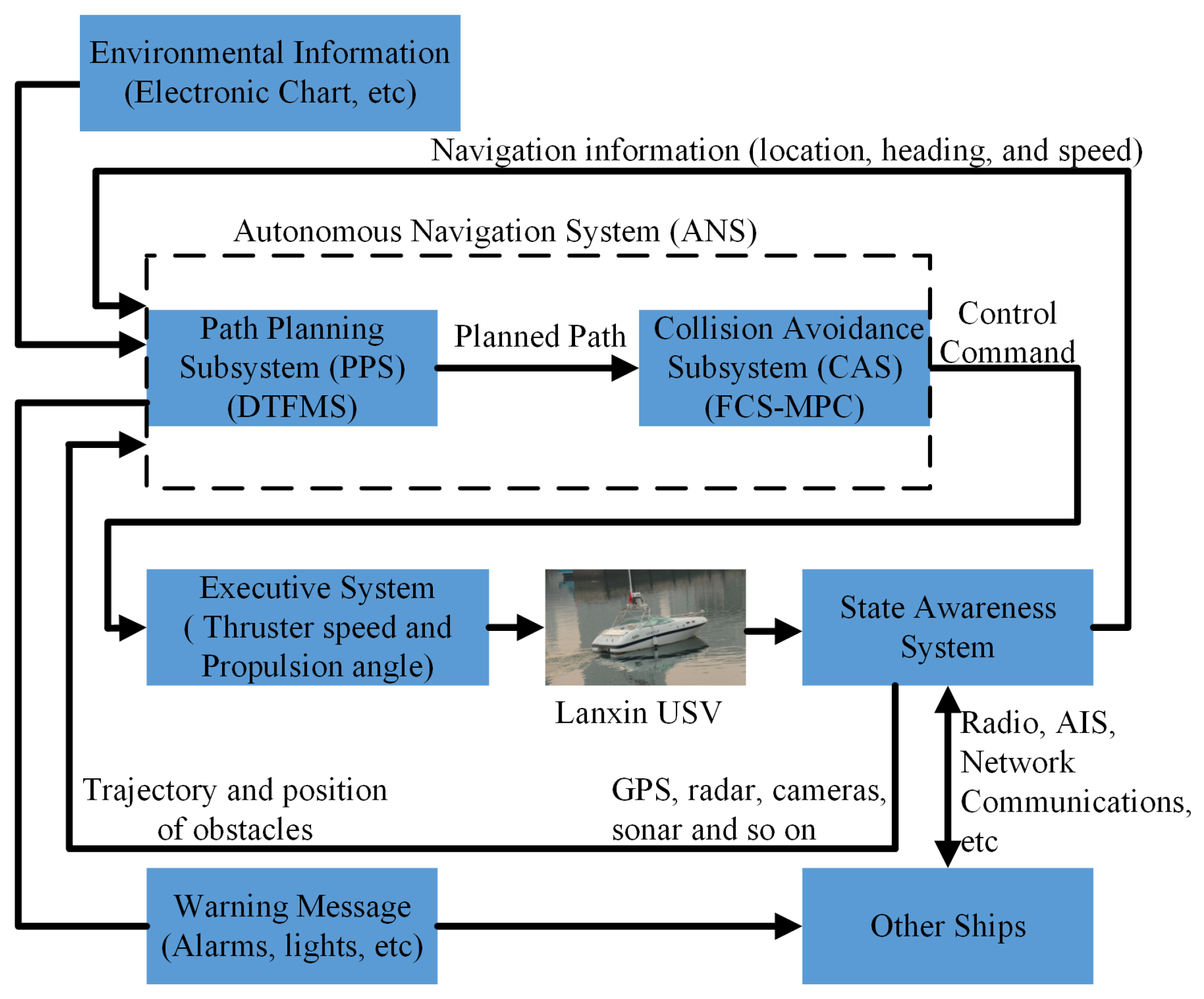
Figure 2.
The simulation environment. (a) The initial binary map; (b) The expanded map.

Figure 3.
The updating process when using the fast marching method (FMM). (a) Initial state; (b) Iteration 1; (c) Iteration 5; (d) Iteration 13; (e) Iteration 25; (f) Iteration 37; (g) Iteration 45; (h) Iteration 49.
Figure 3.
The updating process when using the fast marching method (FMM). (a) Initial state; (b) Iteration 1; (c) Iteration 5; (d) Iteration 13; (e) Iteration 25; (f) Iteration 37; (g) Iteration 45; (h) Iteration 49.

Figure 4.
The fast marching method (FMM) applied over a grid map. (a) One wave source in two dimensions; (b) One wave source in three dimensions; (c) Four wave sources in two dimensions; (d) Four wave sources in three dimensions.
Figure 4.
The fast marching method (FMM) applied over a grid map. (a) One wave source in two dimensions; (b) One wave source in three dimensions; (c) Four wave sources in two dimensions; (d) Four wave sources in three dimensions.
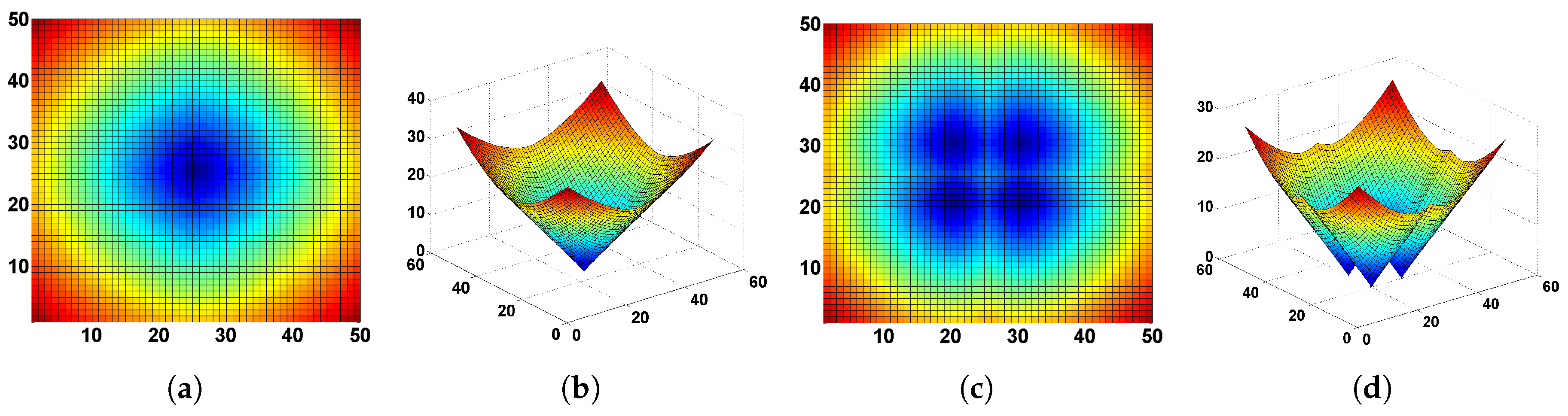
Figure 5.
Path planning with the fast marching method (FMM). (a) Output of the FMM, i.e., arrival time matrix T; (b) Path obtained after applying gradient descent on T; (c) Generated path and arrival time matrix T in three dimensions.
Figure 5.
Path planning with the fast marching method (FMM). (a) Output of the FMM, i.e., arrival time matrix T; (b) Path obtained after applying gradient descent on T; (c) Generated path and arrival time matrix T in three dimensions.
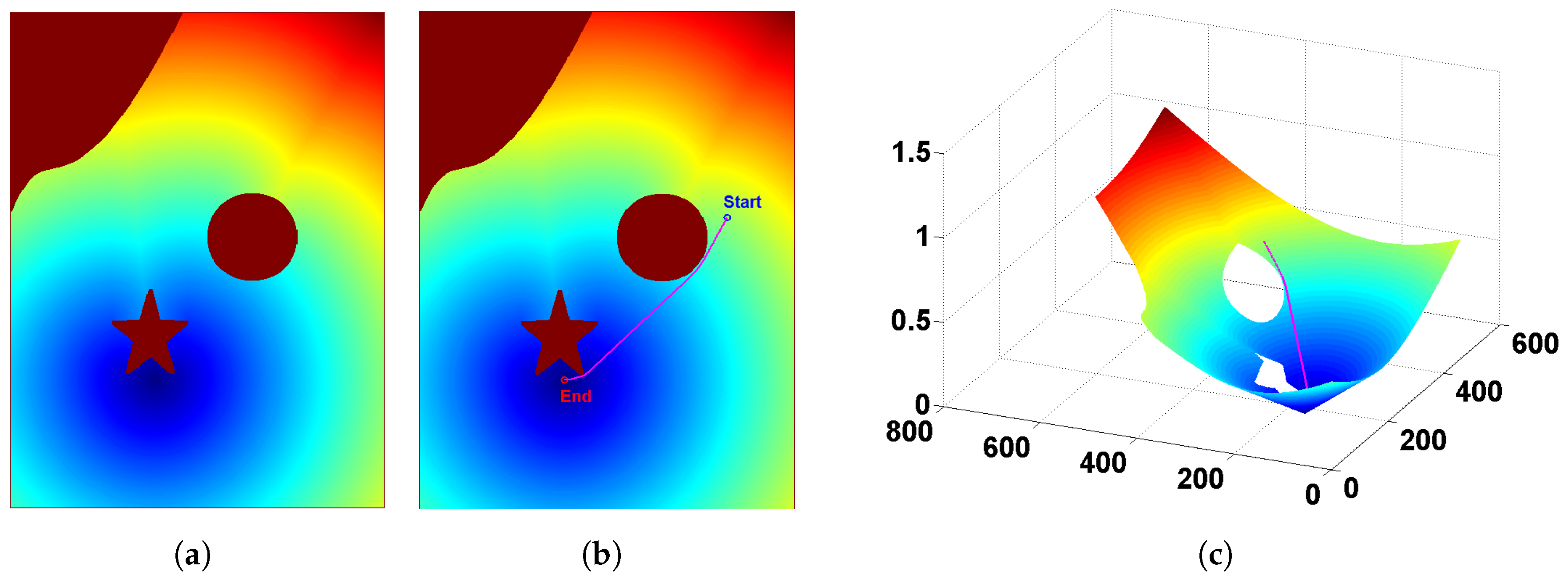
Figure 6.
Path planning with the fast marching square (FMS) method. (a) The safety potential map V; (b) The arrival time matrix T; (c) Path obtained after applying gradient descent on T; (d) Generated path and arrival time matrix T in three dimensions.
Figure 6.
Path planning with the fast marching square (FMS) method. (a) The safety potential map V; (b) The arrival time matrix T; (c) Path obtained after applying gradient descent on T; (d) Generated path and arrival time matrix T in three dimensions.
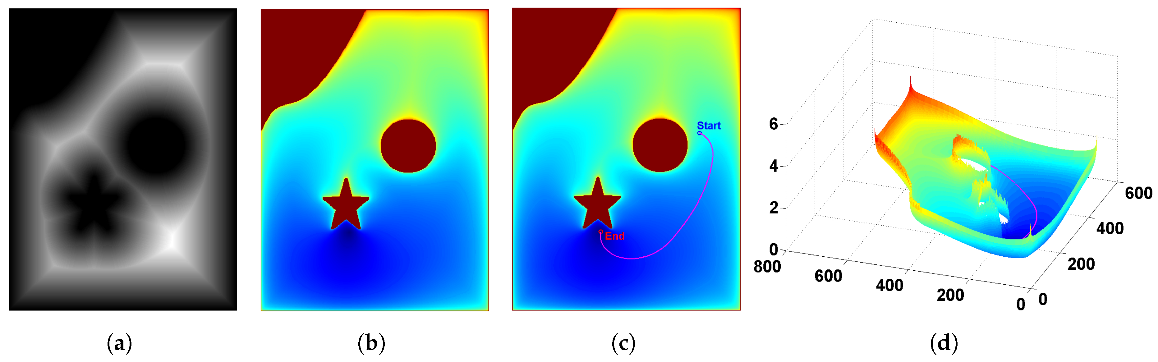
Figure 7.
Path planning with different values. (a) 0.9; (b) 0.7; (c) 0.5; (d) 0.3.
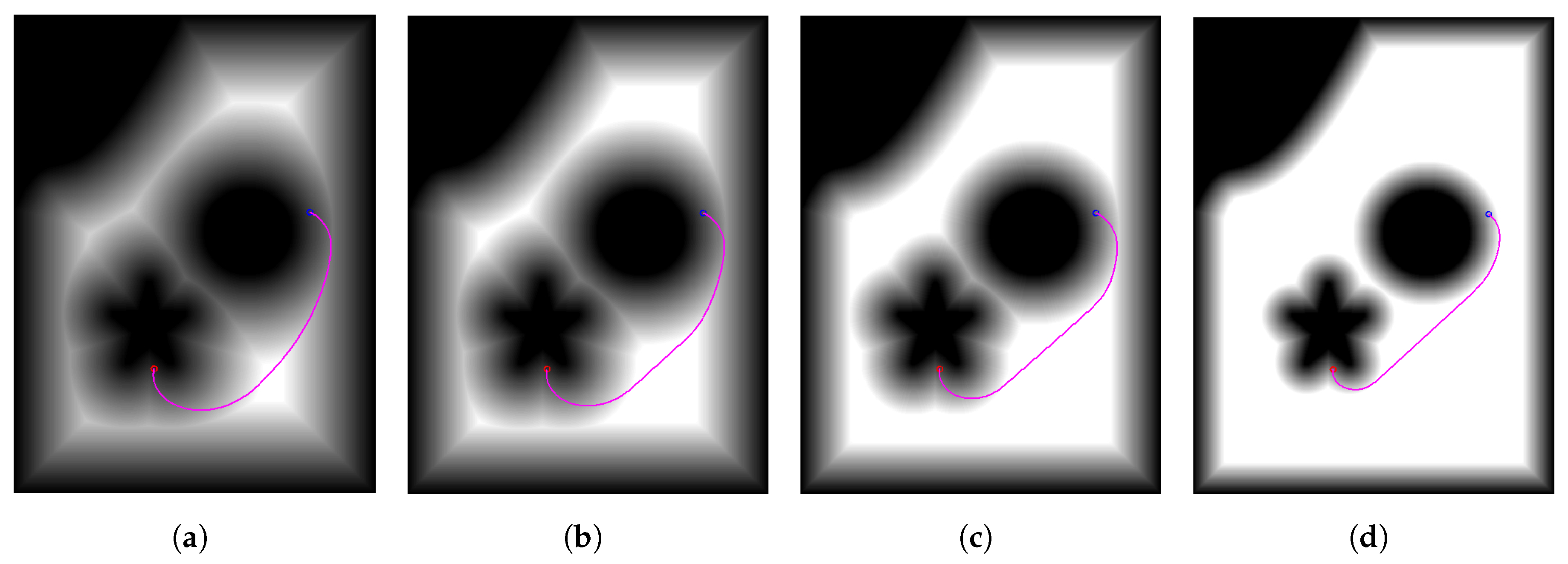
Figure 8.
Steps of the tunable fast marching square (TFMS) method in a real sea area. (a) Electronic chart of the sea area; (b) Initial binary map; (c) Expanded binary map; (d) Potential map V with 0.9; (e) Arrival time matrix T; (f) Path obtained after applying gradient descent on T.
Figure 8.
Steps of the tunable fast marching square (TFMS) method in a real sea area. (a) Electronic chart of the sea area; (b) Initial binary map; (c) Expanded binary map; (d) Potential map V with 0.9; (e) Arrival time matrix T; (f) Path obtained after applying gradient descent on T.
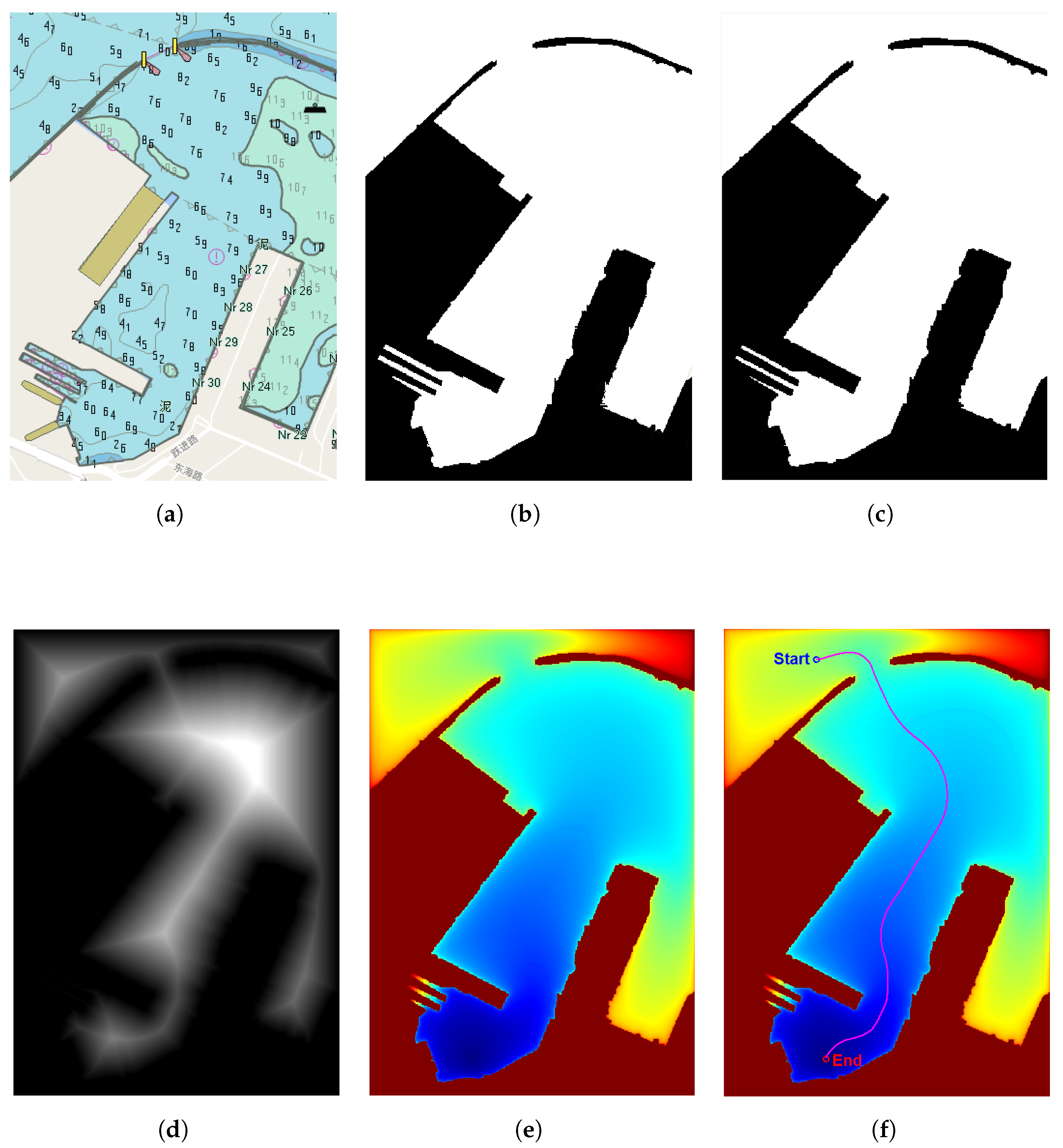
Figure 9.
Block diagram of finite control set model predictive control (FCS-MPC) for the collision avoidance subsystem (CAS). USV: unmanned surface vehicle.
Figure 9.
Block diagram of finite control set model predictive control (FCS-MPC) for the collision avoidance subsystem (CAS). USV: unmanned surface vehicle.

Figure 10.
Description attainability and safety subfunctions in potential map V with 0.9. : the predicted course; : the difference angle between and the navigation angle.
Figure 10.
Description attainability and safety subfunctions in potential map V with 0.9. : the predicted course; : the difference angle between and the navigation angle.

Figure 11.
The unmanned surface vehicle falling into the local optimum in a static simulation environment.
Figure 11.
The unmanned surface vehicle falling into the local optimum in a static simulation environment.
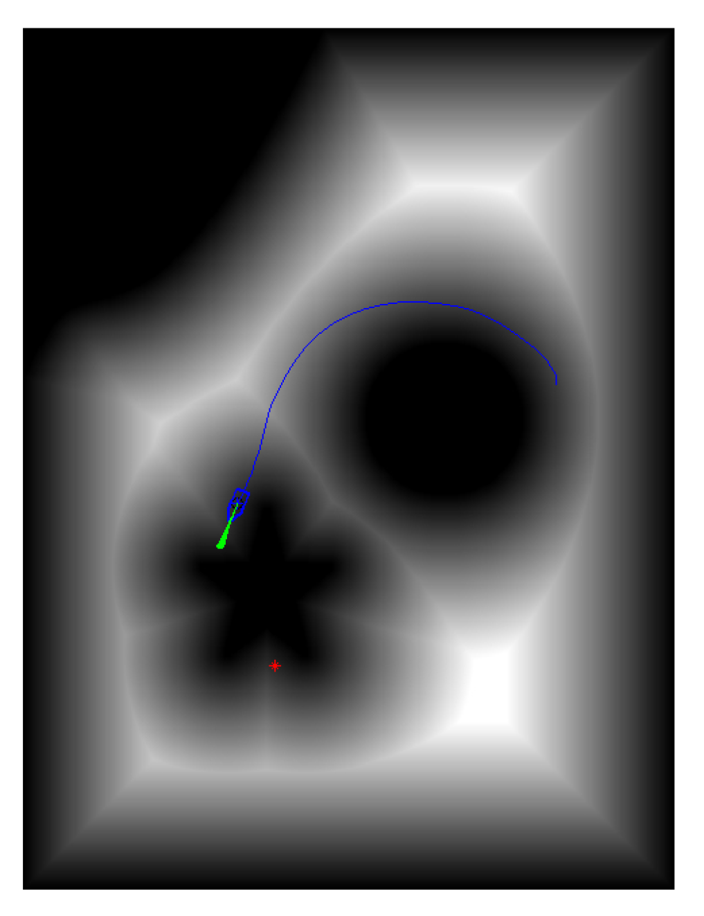
Figure 12.
The own vessel dynamic domain model. (a) Schematic of the own vessel dynamic domain model; (b) The pixel image of domain model with speed 2.5 m/s and included angle of reachable area ; (c) Speed 10 m/s and ; (d) Speed 5 m/s and ; (e) Speed 5 m/s and . : the included angle of reachable area.

Figure 13.
Target vessel dynamic domain model. (a) Schematic of the target vessel dynamic domain model; (b) The pixel image of domain model with speed 2.5 m/s; (c) Speed 5 m/s; (d) Speed 6 m/s; (e) Speed 8 m/s; (f) Speed 10 m/s.
Figure 13.
Target vessel dynamic domain model. (a) Schematic of the target vessel dynamic domain model; (b) The pixel image of domain model with speed 2.5 m/s; (c) Speed 5 m/s; (d) Speed 6 m/s; (e) Speed 8 m/s; (f) Speed 10 m/s.
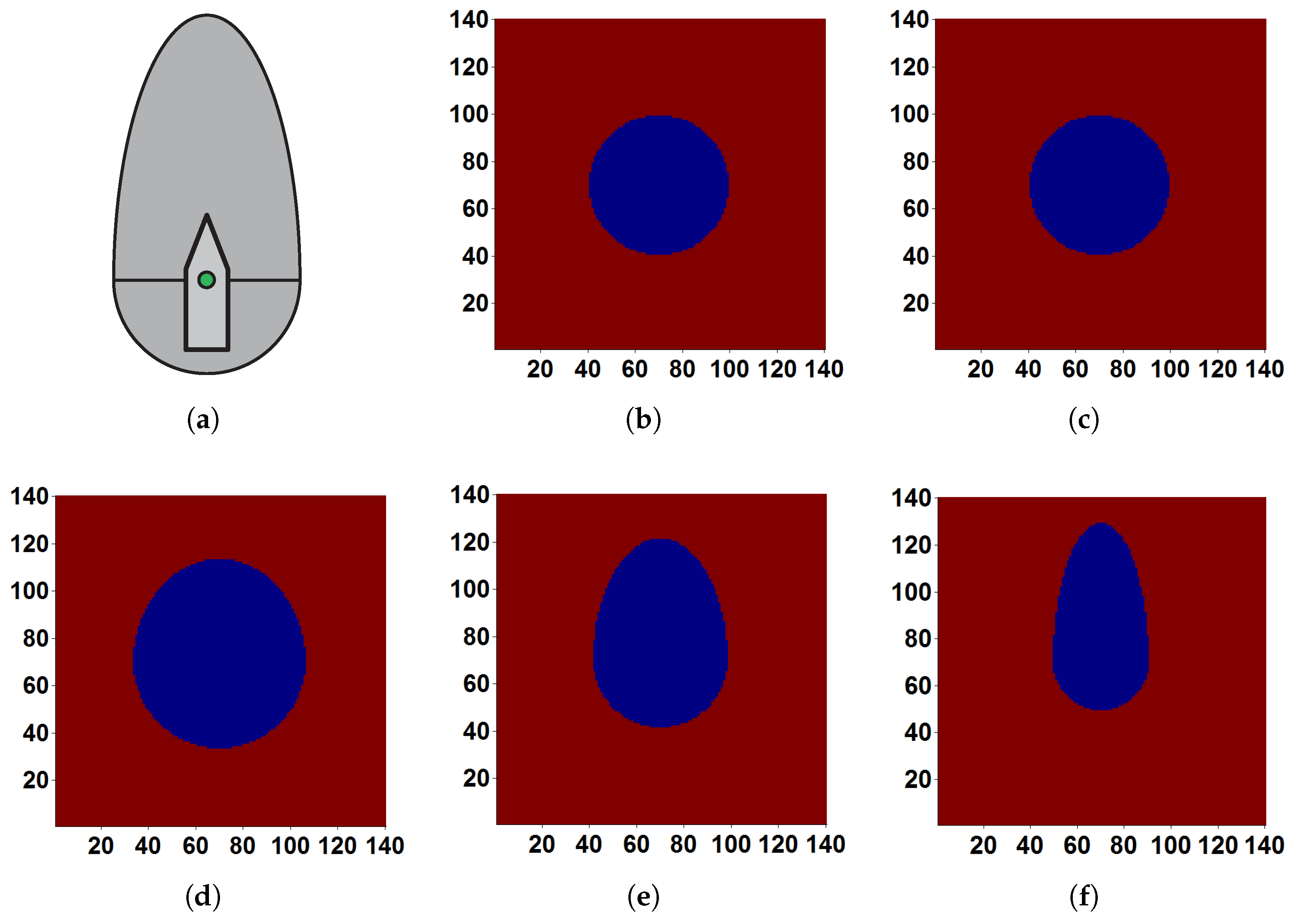
Figure 14.
The outputs of target vessel domain model for increasing speed U with = 4 s, = 20 m, and = 5 m/s. The dotted line represents the output for the bow section, and the solid line represents the stern section of the target vehicle. : minimum radius of the domain model; : the boundary value of speed; : the semi-major axis of the bow part; : the radius of stern part.
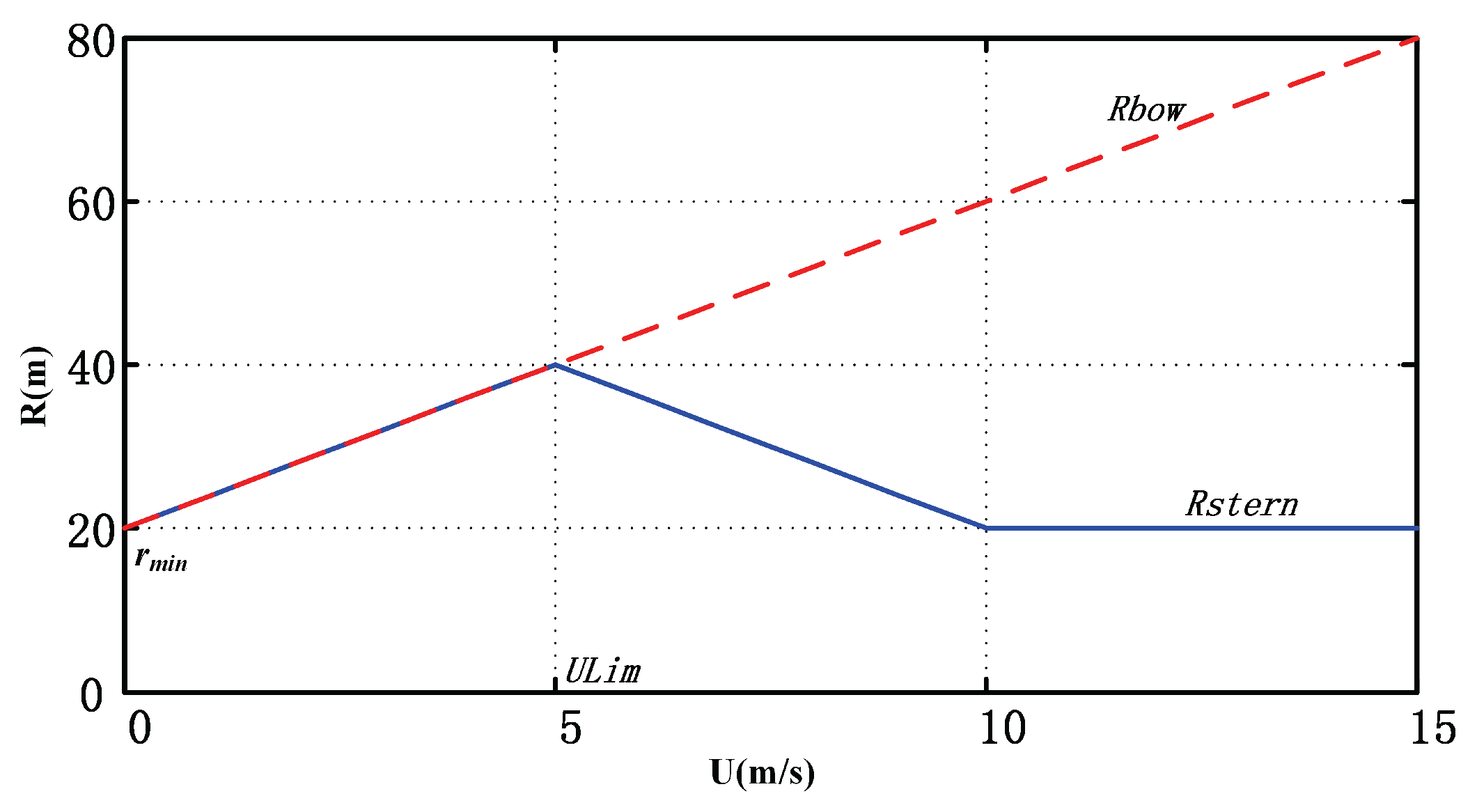
Figure 15.
The process of path re-planning. (a) Addition of domain models to potential map V (time 0.08 s); (b) New potential map by tunable fast marching square (TFMS; time 0.20 s); (c) Generated path and arrival time matrix T (time 0.22 s); (d) Generated path and arrival time matrix T with a single target vessel domain model; (e) Generated path and arrival time matrix T in three dimensions; (f) Single target vehicle domain model in three dimensions.

Figure 16.
Path re-planning in an actual environment. (a) Addition of domain models to potential map V (time 0.30 s); (b) New potential map by tunable fast marching square (TFMS; time 1.80 s); (c) Generated path and arrival time matrix T (time 1.80 s).
Figure 16.
Path re-planning in an actual environment. (a) Addition of domain models to potential map V (time 0.30 s); (b) New potential map by tunable fast marching square (TFMS; time 1.80 s); (c) Generated path and arrival time matrix T (time 1.80 s).
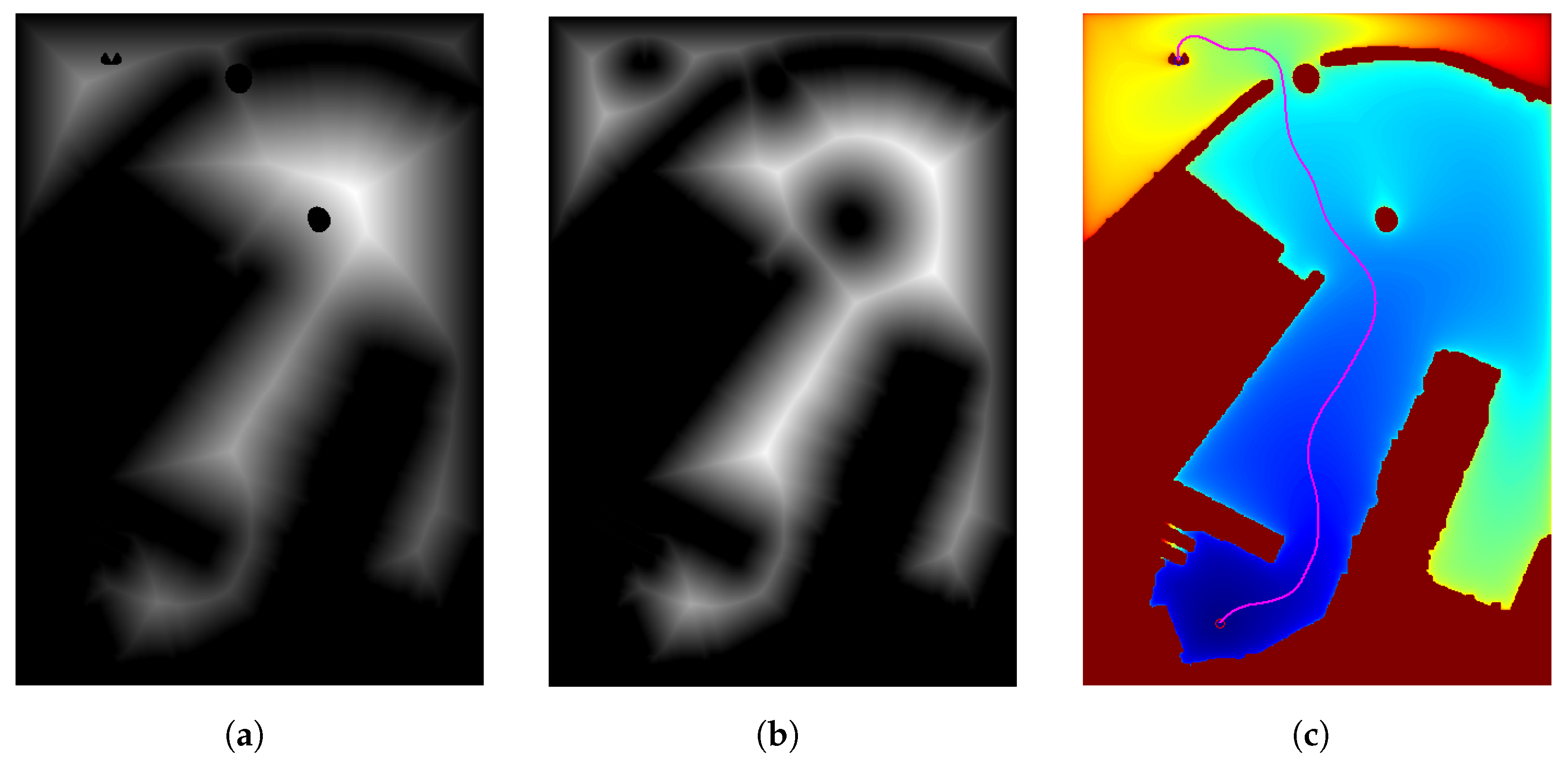
Figure 17.
The simulation final result in a static simulation environment. (a) The binary map; (b) The potential map.
Figure 17.
The simulation final result in a static simulation environment. (a) The binary map; (b) The potential map.
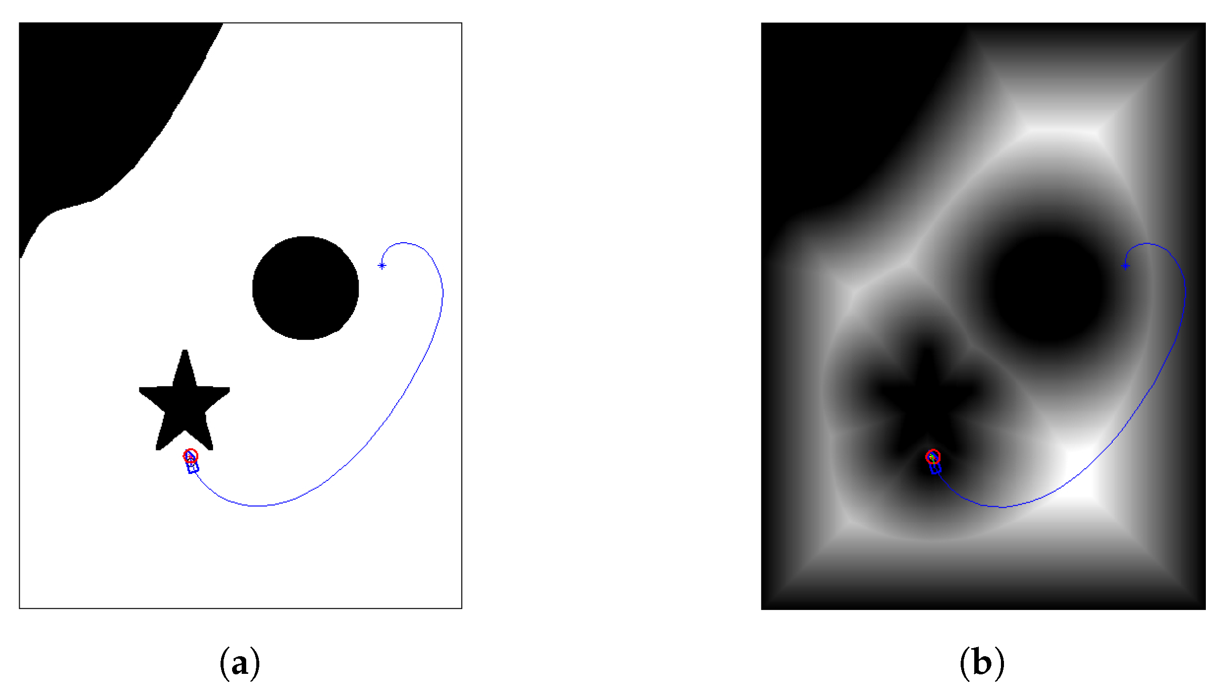
Figure 18.
The motion sequence diagram of the unmanned surface vehicle with single target vessel in the simulation environment. (a) Time 3 s; (b) Time 11 s; (c) Time 20 s; (d) Time 28 s; (e) Time 31 s; (f) Time 34 s; (g) Time 43 s; (h) Time 52 s.
Figure 18.
The motion sequence diagram of the unmanned surface vehicle with single target vessel in the simulation environment. (a) Time 3 s; (b) Time 11 s; (c) Time 20 s; (d) Time 28 s; (e) Time 31 s; (f) Time 34 s; (g) Time 43 s; (h) Time 52 s.
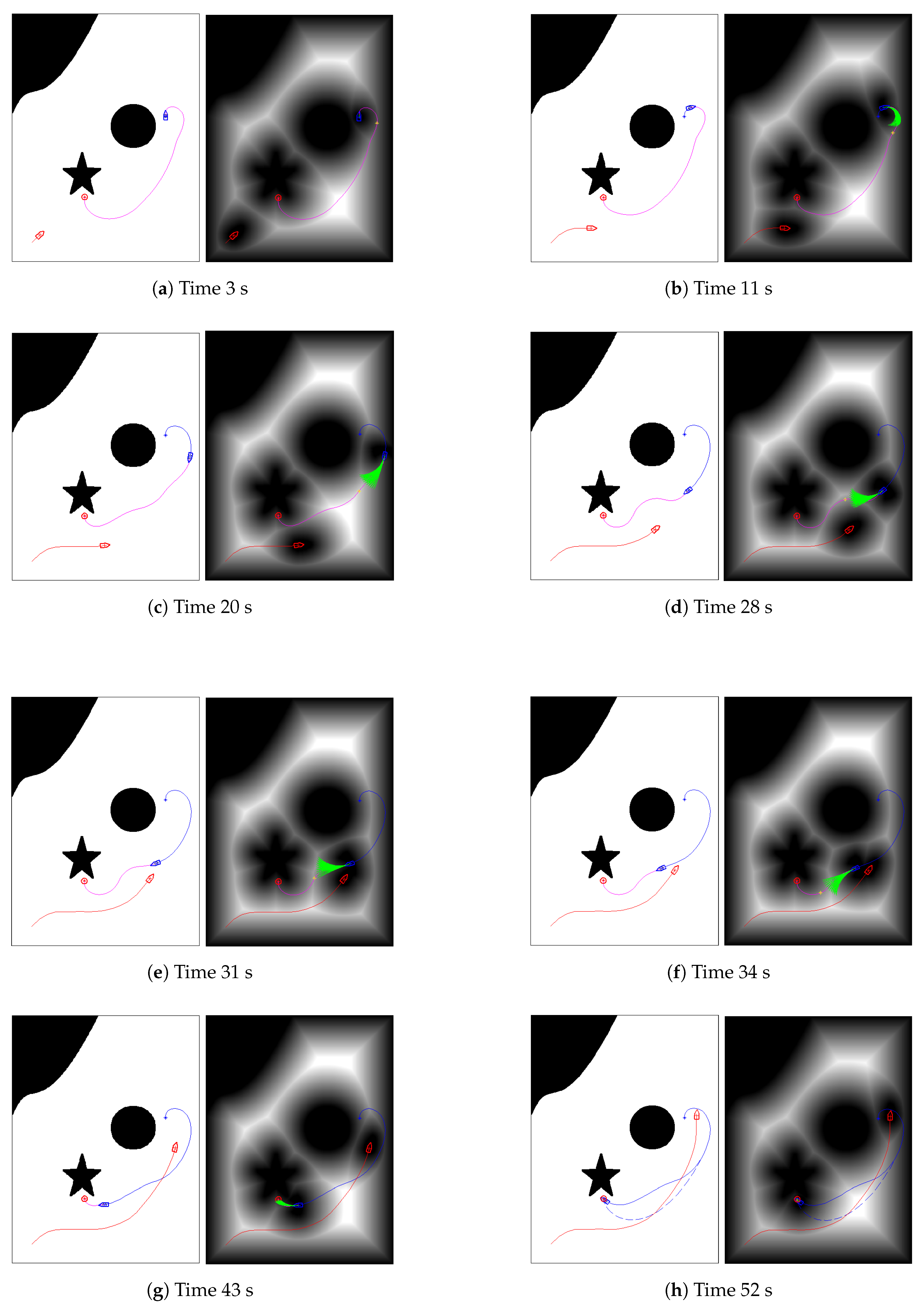
Figure 19.
Evaluation results in the simulation environment. (a) Speed of the unmanned surface vehicle (USV); (b) Course of the USV; (c) Thruster speed; (d) Command propulsion angle; (e) Computation time; (f) Distance between the USV and collision area.
Figure 19.
Evaluation results in the simulation environment. (a) Speed of the unmanned surface vehicle (USV); (b) Course of the USV; (c) Thruster speed; (d) Command propulsion angle; (e) Computation time; (f) Distance between the USV and collision area.

Figure 20.
The simulation final result in static sea environment. (a) The binary map; (b) The potential map.
Figure 20.
The simulation final result in static sea environment. (a) The binary map; (b) The potential map.

Figure 21.
The motion sequence diagram of the unmanned surface vehicle with multiple target vessels in a real environment. (a) Time 5 s; (b) Time 29 s; (c) Time 33 s; (d) Time 37 s; (e) Time 69 s; (f) Time 73 s; (g) Time 77 s; (h) Time 97 s; (i) Time 121 s; (j) Time 137 s; (k) Time 161 s; (l) Time 176 s.

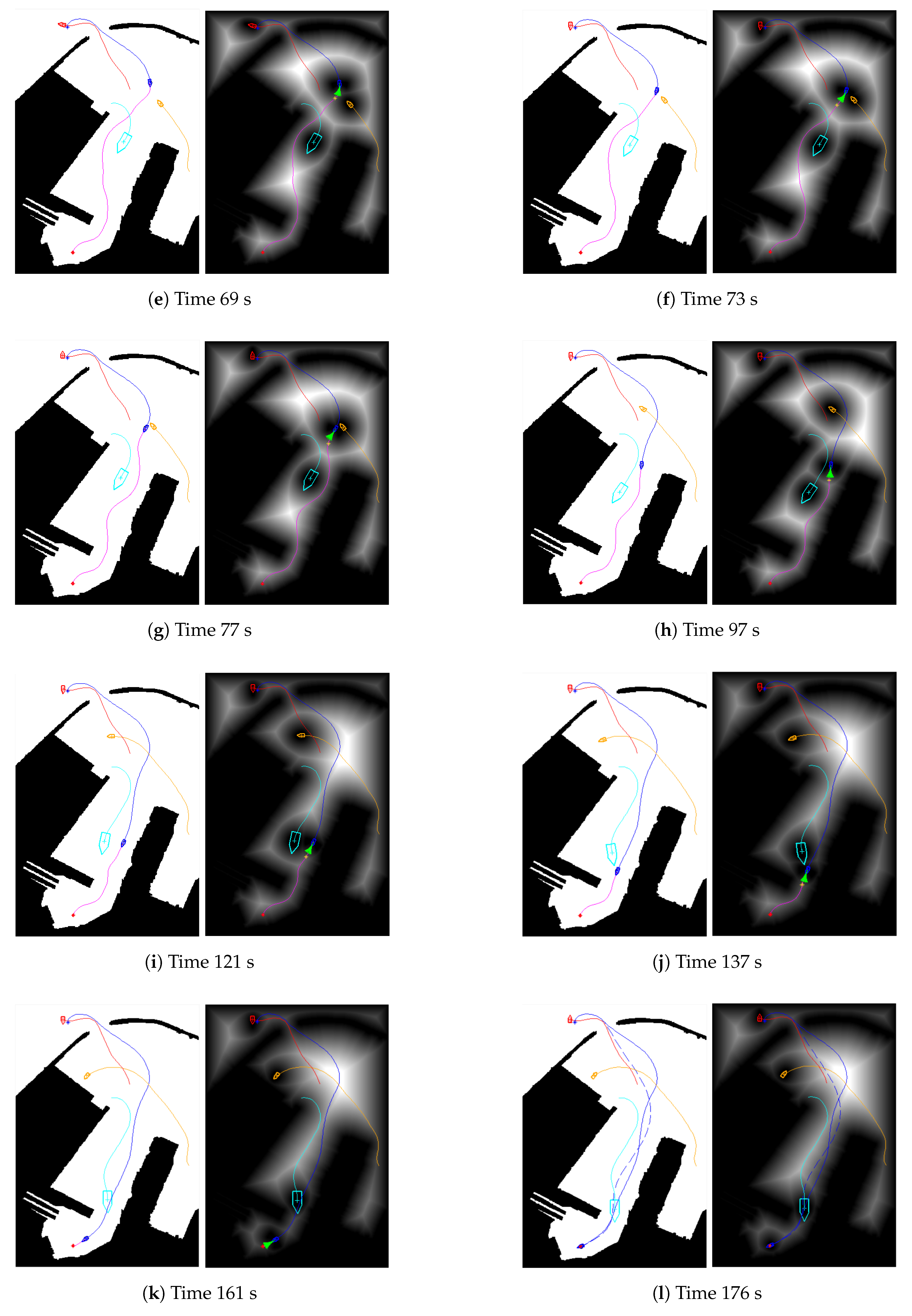
Figure 22.
Evaluation results in the real environment. (a) Speed of the unmanned surface vehicle (USV); (b) Course of the USV; (c) Thruster speed; (d) Command propulsion angle; (e) Computation time; (f) Distance between the USV and the collision area.
Figure 22.
Evaluation results in the real environment. (a) Speed of the unmanned surface vehicle (USV); (b) Course of the USV; (c) Thruster speed; (d) Command propulsion angle; (e) Computation time; (f) Distance between the USV and the collision area.


Table 1.
Parameter information about the automatic navigation system (ANS) of the unmanned surface vehicle (USV).
Table 1.
Parameter information about the automatic navigation system (ANS) of the unmanned surface vehicle (USV).
| Parameter | Value | Units | |
|---|---|---|---|
| USV | Size of the USV (length, breadth) | (7.02, 2.60) | m |
| Initial course of the USV | 90.0 | ||
| Initial speed of the USV | 0.0 (0.0) | m/s (kn) | |
| Initial thruster speed | 0.0 | r/min | |
| Maximum thruster speed | 66.7 (4000) | r/s (r/min) | |
| Change rate of thruster speed | 6.7 | r/s | |
| Discrete thruster speed | 1.7 (100) | r/s (r/min) | |
| Initial propulsion angle | 0.0 | ||
| Maximum propulsion angle | 30.0 | ||
| Change rate of propulsion angle | 5.0 | /s | |
| Discrete propulsion angle | 1.0 | ||
| Algorithm | 0.9 | – | |
| Search range | 100.0 | m | |
| Prediction horizon | 8.0 | s | |
| Control update interval | 1.0 | s | |
| Weight of evaluation function | (1.50, 1.50, 0.01, 2.00) | – |
Table 2.
Results of evaluation index comprised of two tests in the simulation environment. USV: unmanned surface vehicle.
Table 2.
Results of evaluation index comprised of two tests in the simulation environment. USV: unmanned surface vehicle.
| Environment | Index | Speed of the USV (m/s) | Thruster Speed (r/min) | Propulsion Angle (°) | Computation Time (s) | Distance (m) |
|---|---|---|---|---|---|---|
| static | maximum | 11.0 | 4000 | 0.0 | 0.63 | 100.0 |
| minimum | 0.0 | 0 | −30.0 | 0.11 | 19.8 | |
| average | 7.5 | 3109 | −10.8 | 0.25 | 51.1 | |
| dynamic | maximum | 10.9 | 4000 | 3.0 | 0.61 | 86.8 |
| minimum | 0.0 | 0 | −30.0 | 0.11 | 10.4 | |
| average | 7.2 | 3059 | −10.5 | 0.26 | 35.9 |
Table 3.
Results of evaluation index comprised of two tests in real environment. USV: unmanned surface vehicle.
Table 3.
Results of evaluation index comprised of two tests in real environment. USV: unmanned surface vehicle.
| Environment | Index | Speed of the USV (m/s) | Thruster Speed (r/min) | Propulsion Angle (°) | Computation Time (s) | Distance (m) |
|---|---|---|---|---|---|---|
| static | maximum | 11.0 | 4000 | 2.0 | 0.27 | 100.0 |
| minimum | 0.0 | 0 | −18.0 | 0.14 | 60.8 | |
| average | 10.0 | 3731 | −1.9 | 0.16 | 92.8 | |
| dynamic | maximum | 11.0 | 4000 | 2.0 | 0.27 | 100.0 |
| minimum | 0.0 | 0 | −18.0 | 0.15 | 25.4 | |
| average | 9.9 | 3690 | −1.9 | 0.17 | 85.7 |
© 2018 by the authors. Licensee MDPI, Basel, Switzerland. This article is an open access article distributed under the terms and conditions of the Creative Commons Attribution (CC BY) license (http://creativecommons.org/licenses/by/4.0/).
Share and Cite
MDPI and ACS Style
Sun, X.; Wang, G.; Fan, Y.; Mu, D.; Qiu, B. An Automatic Navigation System for Unmanned Surface Vehicles in Realistic Sea Environments. Appl. Sci. 2018, 8, 193. https://doi.org/10.3390/app8020193
AMA Style
Sun X, Wang G, Fan Y, Mu D, Qiu B. An Automatic Navigation System for Unmanned Surface Vehicles in Realistic Sea Environments. Applied Sciences. 2018; 8(2):193. https://doi.org/10.3390/app8020193
Chicago/Turabian StyleSun, Xiaojie, Guofeng Wang, Yunsheng Fan, Dongdong Mu, and Bingbing Qiu. 2018. "An Automatic Navigation System for Unmanned Surface Vehicles in Realistic Sea Environments" Applied Sciences 8, no. 2: 193. https://doi.org/10.3390/app8020193
Note that from the first issue of 2016, this journal uses article numbers instead of page numbers. See further details here.