Operation Loop-Based Optimization Model for Resource Allocation to Military Countermeasures versus Probabilistic Threat


College of Systems Engineering, National University of Defense Technology, Changsha 410073, China
*
Author to whom correspondence should be addressed.
Appl. Sci. 2018, 8(2), 214; https://doi.org/10.3390/app8020214
Submission received: 21 November 2017
/
Revised: 12 January 2018
/
Accepted: 26 January 2018
/
Published: 31 January 2018
Abstract
:Weapons development planning is an unstructured and complex multi-criteria decision-making problem, especially in antagonistic environments. In this paper, the defender’s decision was modelled as a high complexity non-linear optimization problem with limited resources. An operation loop with realistic link rules was first proposed to model the cooperation relationships among weapons in the defense system. The system dynamics principle was used to characterize the dynamic behavior of the nodes in a complex weapons network. Then, we used cumulative threat and development risk to measure different planning solutions by considering the opponent and uncertainties in the development process. Next, an improved Differential Evolution (DE) and Non-Dominated Sorting Differential Evolution (NSDE) were designed to determine the optimal planning solutions for a single objective and multi-objective. The compromise solution, based on the Technique for Order Preference by Similarity to an Ideal Solution (TOPSIS), was used to evaluate the Pareto solution set of the multi-objective. Finally, an illustrative case was studied to verify the feasibility and validity of the proposed model.
1. Introduction
After the 11 September 2001 terrorist attacks on the World Trade Center and the Pentagon in the United States, interest in counter-terrorism methods with limited resources has rapidly increased. However, allocating scarce defensive resources to optimize an objective function is one of the classic problems in Operations Research [1], being an important and difficult task [2]. For the defense agencies in many countries, weapon system of systems (WSOS) development planning is a critical process used to develop countermeasures (CMs) to confront the threats posed by other hostile countries [3]. The planning solution focuses on how to allocate resources to different weapons to effectively eliminate the threat from hostile countries.
In prior studies on weapons development planning, a decision maker (DM) seeks to maximize a single objective function, such as capability, profit, and effectiveness. For example, Gu et al. [4] established a WSOS planning model by maximizing the expected effectiveness as the optimization target. Håkenstad [5] compared the long-term defense planning systems of seven Nordic countries and found that most countries aimed to improve their own profit. Zhang et al. [6] proposed an optimization model to minimize the capability gaps to find the best development scheme by comparing different combinations of weapons, based on the given capability requirements. Throughout the literature research, however, did not mention the change of the opponent. In contrast, this paper considered minimizing the threat caused by the enemy as the objective function. Herein, we addressed an arms race between two parties, R and B. Each party considers the potential threat from the other party. R develops one or more weapons to gain operational advantages over B, whereas B attempts to develop one or more CMs that would neutralize, or at least mitigate, the threat from R [7].
Resource allocation in adversarial settings, also called the research of arms races using mathematical models, has been studied since the 1930s. However, most of these studies focused only on the strategic aspect but not the operational aspect. In 1935, Richardson [8] first proposed a simple coupled differential equation model to solve the effects of an arms race between rival states, thus successfully predicting World War II. Later, Hunter [9] analyzed a three-nation arms race by solving linear difference equations based on Richardson’s study. Similar to most previous research, Hunter’s model focused only on the strategic aspect and did not consider the relationship between research and development (R&D) investments and time, nor the cooperation relationships among different weapons. Afterwards, Etcheson [3] established and solved equations to optimize the function of each side rather than the constrained nonlinear optimization model. Recently, Paulson et al. [10] proposed a model for determining optimal resource allocation by combining game theory with a simple multi-attribute utility model. The defender first allocated her resources amongst all combinations of countermeasures and targets, and then the attacker striked with his best response to this allocation. Golany [11] investigated efficient computation schemes for allocating two defensive resources to multiple sites to protect against possible attacks by an adversary. The availability of the two resources was constrained and the effectiveness of each may vary over the site. Mazicioglu [12] modelled the attacker’s behavior using multi-attribute prospect theory to account for the attacker’s multiple objectives and deviations from rationality. These articles mainly modelled adversary’s behavior from macroscopic and strategic view, and considered neither the time required to develop new countermeasures, nor the relationship between expenditures and development gap. In addition, budgets were not modelled explicitly.
WSOS is a variety of weapons that can be functionally related to each other in accordance with a certain structure with a higher level of integration with certain strategic guidance, operational command, and security conditions [13]. Moreover, with the development of technology, the operational effectiveness of an army depends on the interactions between multiple weapons instead of independent weapons [14]. However, to the best of our knowledge, the relationships among different weapons have rarely been modelled in the literature. For example, the most authoritative article in Operations Research [15] focused only on a single family of countermeasures (e.g., interception systems or bomb neutralization systems) that evolves and improves over time. With the development of informationization, the performance of defense depends on the interaction of multiple systems rather than the individual attributes of the armaments. As a consequence, the defender tends to use several families of CMs instead of a single type, so the performance of the defense cannot be determined only by the effectiveness of any single CM employed. Instead, the cooperation between CMs should be considered. Furthermore, as new CMs are introduced, even in the decision-making stage, the defender may also have to consider the interaction between the current CMs and future possible CMs to optimize the defense system. If the relationships among weapons are ignored in the development planning process, the problem will be simplified to a simple selective problem of a single weapon, neglecting the holistic structural characteristics [16]. Thus, we used and improved an operation loop-based network model focusing on the cooperation relationships among the weapons [17], in which weapons are represented as nodes, whereas relationships among the weapons are modelled as edges. In this model, weapons entities contain sensor, decision, influencer, and target nodes. All types of nodes are treated as target nodes to the enemy. Note that one weapon may be characterized as multiple nodes, and each node is attached to a parameter, denoting the amount of the resources allocated to it. In addition, we considered the real link rules of these nodes that prior studies [18] did not mention. For example, if more than one S node exists in one operation loop, the nodes could only be arranged based on their index values of Radius in descending order. Due to the limitation of the geographical locations of the different weapons and some other factors, not all nodes could transfer information or energy, and certain nodes could only be arranged in descending or ascending order. This phenomenon is common in real-life operational battles.
In summary, this problem can be modelled as a constrained nonlinear optimization problem, which is known as NP-hard. The complexity of this type of problem depends on the complex relationships among weapons. Consequently, we argue that the analytical solution to the problem is not feasible, and a heuristic-based optimization algorithm would be effective. In this article, we used Differential Evolution (DE) and Non-Dominated Sorting based Genetic Algorithm-II (NSGA-II) for our optimization tasks.
The main contributions of this paper are as follows: (1) When assessing the threat posed by the enemy, we not only considered the cooperation among different nodes based on the traditional ideology of the operation loop, but also the real link rules of these nodes. Meanwhile, the system dynamics principle was used to characterize the dynamic behavior of the nodes in the complex weapons network; (2) According to the characteristics of the weapon life cycle curve, we considered some realistic constraint conditions, such as the annual weapons budget, the total weapons budget, and the weapon planning cycle; (3) A complex multi-objective planning problem and the related solving approach were proposed, considering the development risks and probabilistic threat from the enemy. In this paper, we considered practical settings in realistic dynamic competition.
This paper was organized as follows. Section 2 introduced the modeling method based on operation loop and the threat assessment process. Section 3 elaborated upon the single objective optimization model with time and investment constraints. In addition, the algorithm to solve the problem was outlined. Section 4 extended the objective functions to an actual weapons R&D process. Section 5 demonstrated the usefulness of the models by presenting the results of a numerical experiment. Finally, Section 6 concluded the paper and discussed possible future research.
2. Problem Formulation
Throughout history, two or more countries are often in hostilities, such as the United States and the Soviet Union during the Cold War, India and Pakistan, and so on. Therefore, WSOS development planning transforms from a capacity to a military demand, as seen as an arms race. The R&D of national military weapons occurs in a situation requiring rapidity of development. Each country will set the other country or countries as the “reference” or “opponent” and change their own R&D strategies following the change of the R&D strategies of the opponent. Herein, we considered the dynamic competition between two parties, denoted as the attacker (R) and the defender (B). Generally speaking, R is a military power with advanced military technology and in a leading position in the military. R will independently develop a set of new weapons early on to attack B to gain an advantage at time tR1. The weapons developed by R are targets that B must counter. If all information about R is obtained by the intelligence department of B completely and opportunely at time tR1, then the initial damage (d1) caused by R, typically measured in casualties and economic damages [15], to B is known. As shown in Figure 1a, to defend the homeland from being attacked by R, B must develop new weapons (Bn) as CMs to mitigate the damage. However, as shown in Figure 1b, if B cannot intercept information about R’s new weapon or B’s CMs fail, the threat will remain.
The collection of different weapons is called WSOS. Modern weapons are complex, integrated, and diverse. The connections among weapons also vary. Therefore, we not only considered interdependency among the current weapons, but also relationships among all current and future weapons. In this paper, the concept of meta-functional nodes and meta-functional edges, based on the operation loop, was used to model the cooperation relationships among weapons.
2.1. Cooperation Relationships Modeling among Weapons Based on an Operation Loop
2.1.1. Meta-Functional Node Modeling
A meta-functional node can be represented as a three tuple, containing a node identity, node type, and node threat vector, as shown below:
The node identification indicates the position of the meta-functional node in combat operation process, such as red or blue. The node type refers to the classification of the meta-functional node, which can be divided into different categories from different angles. Cares [19] divided nodes into sensor, decider, influencer, and target according to the different roles on the battlefield. In this study, meta-functional nodes were divided into four categories: scout, command-and-control, influence, and target, which are expressed as follows:
where S, D, I and T represent the meta scout functional node, meta command-and-control functional node, meta influence functional node, and meta target functional node, respectively. Node S refers to the weapon, equipment, entity, or system that performs basic surveillance, reconnaissance, and warning in a battle, such as radar and infrared detection systems. Node D is a system that performs basic command and control tasks during a combat operation. Node I is a device, entity, or system that performs basic fire strikes or electromagnetic interference during a battle, such as artillery, missiles, and torpedoes. Different nodes are included in both the same and different weapons. For example, an armored observation and command vehicle can be characterized as node S and node D. A self-propelled antiaircraft gun can only be characterized as node I. An illustrative example of different nodes in WSOS is provided in Figure 2. Different parties are described with corresponding color. R has five existing nodes (S1, D1, D2, D3 and I2) and one new weapon (S2) awaiting development. S1, S2 and I2 can be detected by B and become B’s targets. The same applies to the other party.
2.1.2. Meta-Functional Edge Modeling
Considering the antagonism between the two sides, B will set all of R’s nodes as the target. Similarly, R will set all of B’s nodes as the target. Thus, 36 (node number × node number) different combinations of the three kinds of meta-functional nodes exist. Some types of meta-functional edges, however, do not exist in practical operation. Based on the following assumptions, we filtered the 36 edge types: (1) the node S cannot act independently; it can only share information with other S or D nodes; (2) the node D cannot attack the enemy target directly; and (3) the node I will not interfere or attack its own weapons. After applying these filters, 20 edge relationships remained in the WSOS network under the antagonistic situation, as shown in Table 1.
2.1.3. Operation Loop Modeling
Modern warfare theory, which is also called Observe Orient Decide Act (OODA) theory [20], argues that a combat operation is a cyclic process. First is target discovery (T→S), then information is delivered to the node D (S→D). Next, node D analyzes the battlefield situation and charges node I (D→I) to attack node T (I→T). The close loop (T→S→D→I→T) is called the operation loop [21]. During the operation, both parties build their own operation loops, and treat all the opponent’s nodes as targets, as shown in Figure 3. Although only four classes of meta-functional nodes exist in one operation loop, each type of node can contain more than one weapon. Different weapons cooperate with others through loops. The number and technical performance of loops directly impact the combat effectiveness. The greater the number of loops, the stronger the threat capability. The fewer the nodes and edges in a loop, the better the threat effect.
2.2. Threat Assessment
2.2.1. Node Threat Vector
In this study, we applied the concept of accumulative damage presented by Golany [15], which is an objective function that measures the threat posed by the opponent. To assess the threat of the whole WSOS, we first analyzed the node threat vector. Different types of nodes have different functions, and the corresponding threat vectors vary considerably. Based on prior studies [22,23,24], we improved the index system of different nodes. The threat vector of the node S is:
where Radius, Accuracy, DetectRate and HavestRate denote the reconnaissance scope, the target recognition accuracy, the effective detection rate, and the critical intelligence acquisition rate of the node S, respectively. The threat vector of the node D is
where CoverRate, Efficiency, Community and Dlay represent the effective coverage rate, the information processing efficiency, the network communication efficiency, and the command decision time of the node D, respectively. The threat vector of the node I is
where Radius, Accuracy, RPG and Mobility indicate the operational coverage radius, the hitting accuracy, the ammunition quantity, and the maneuvering speed of the node I, respectively. means that the vector can be extended to different weapons.
2.2.2. Tactical and Technical Index Normalization
The different indicators have different dimensions. For example, the unit of the operational coverage radius is km, and the unit of the maneuvering speed is km/h. Therefore, different index values have to be standardized. The quantitative indexes are divided into two categories: the benefit type and the cost type. The greater is the value of the benefit index, the greater is the threat. The greater is the value of the cost index, the lesser is the threat. For example, the higher is the hitting precision of the node S, the os higher the threat. The shorter is the decision time of the node D, the sooner the attack can be implemented, resulting in a greater threat. The processing methods of the two quantitative indicators are as follows:
where Equation (6) is the standardized function of the dimensionless benefit index and Equation (7) is the standardized function of the dimensionless cost index. I is the original index. Imax and Imin are the worldwide maximum and minimum values of the current index, respectively. As for the benefit index, if the value of I reaches Imax, the score of the index is 1. Otherwise, the score is 0. The same logic applies to the function symbol of the cost index.
2.2.3. Threat Assessment Based on Operation Loop
The basic goal of the WSOS is to strike the opponent targets and reduce the opponent combat capability, until that capability is completely lost. Hence, threat assessment should emphasize the influence on enemy targets. Each operation loop in the WSOS represents a method to strike the enemy target. As a result of the differences in the performance of the weapons within the operation loop, the threat to enemy targets varies. After normalization of the index value, we classified and aggregated the threat value of the various nodes. The weighted sum method was used in this paper, as it is the most commonly used index aggregation method. The method assigns weight wj to each index, and then weights the sum to obtain the threat value dj of one node.
An operation loop contains the node set S, the node set D, and the node set I. The threat to the opponent target of the entire operation loop is
where ds, dd, and di represent the threat vector aggregation value of node S, node D, and node I, respectively. The total threat to the opponent is the sum of all loops.
2.2.4. Initial Threat Rate and Threat Accumulation
The goal of the development of new weapons is to reduce the threat from the opponent. The threat that changes over time is determined by the performance of one’s own weapons. For example, Figure 4 shows the dynamic change in the threat from R during the development process of B. The horizontal axis represents time and the vertical axis represents the threat. The red squares represent the deployment of R’s weapons and the blue dots represent the deployment of B’s weapons. The threat from R increases after R’s new weapon R1 is deployed. Then, the threat accumulates for a period of time. Once B has developed new weapons against R, R’s threat level decreases. Then, R develops new weapons to increase the threat again. That is to say, the threat changes with the deployment of new weapons, and accumulates over time. B selects B1, B2, and B3 from the optional weapons collection. B1 and B2 form operation loops that cover R with other weapons, and the threat from R decreases. Although B develops B3, it cannot form an operation loop that covers R. Therefore, the threat from R remains unchanged.
In summary, B must choose the most suitable weapons against R, and rationally plan the development. In addition, weapons must be deployed as soon as possible to neutralize the threat that accumulate with time.
2.2.5. Evaluation of Threat Reduction Effects
According to the real-life military operations, B develops new weapons to form operation loops to mitigate the threat from R. The number of operation loops represents the number of ways in which the opponent targets can be attacked. The higher the number of operation loops, the more ways are available to cover the opponent target nodes, and the better the threat reduction effect.
The WSOS network is complex dynamical network system. To research this kind of problem, the dynamical theory is usually introduced into the nodes of the complex network. In a complex network, the dynamic behavior of each node is governed by two factors: the original dynamic behavior mechanism of the node itself, and the influence of the nodes to which they are connected. Considering a complex dynamical network system that is coupled to N nodes, the general expression is [25]:
where denotes the state of node vi at time t; f(xi(t)) denotes the primitive dynamic behavior of node vi; c is the coupling coefficient; g(xj(t)) denotes one coupling function through the coupling relationships among nodes; and A = (aij)N×N is the topological structure or adjacency matrix of the complex network, and every element is positive. If aij = 0, no connection exists between node i and node j. Conversely, if aij ≠ 0, a relationship between node i and node j exists. Next, we combined the actual nature of the WSOS to establish a dynamic WSOS network model based on the general model.
From the analysis of the operational process outlined in Section 2.2.4, we knew that the formation of the operation loop of B reduced the threat from R. As a result, the coupling coefficient c was −1. The coupling function g(xj(t)) was calculated using Equations (8) and (9). We assumed that the number of new operation loops was m during B’s weapons development process, and only the operation loops that covered R’s threat nodes reduced the threat from R. Thus, not all m operation loops reduced the threat from R. The value of aij has the following two forms:
In summary, the cumulative threat (DB) expression is:
where denotes the threat from the entire WSOS of R at time t; f(x(t)) denotes the initial threat caused by R, namely, the situation where B’s confrontation is not considered; and denotes a measure of threat reduction.
3. Single Objective Modeling and Solving
Golany [7] viewed an arms race as a process between two asymmetrical groups. The advantage established by one side is temporary, and the advantage disappears when the other side exceeds it. Therefore, the issue faced by B is how to use limited resources to develop effective CMs to mitigate the threat from R as much as possible. Thus, the cumulative threat is used as the optimization objective function. To simplify the computation, we only considered the operation loops that cover the threat nodes of R. Consequently, aij is removed from the expression. Then, all new m loops work to counter R. The initial threat from R is set as d1. The entire duration of the confrontation is expressed as T. The number of B’s operation loops that cover R is m, and the moment of forming of the jth loop is tj. Then, the cumulative threat expression is:
3.1. Constraints
In the WSOS development planning process, B must consider the following two constraints: time and money.
3.1.1. Time
The cumulative threat posed by R gradually increases over time. Supposing B chooses to develop 10 new weapons. If all investments are made at time 0, then the optimal choice is that the development of the 10 new weapons is initiated at time 0. Therefore, B can deploy new weapons to counter R more rapidly. If not all investments are made simultaneously, but in batches due to the limited investments amount for each batch, B must consider the sequence of these new weapons. Therefore, the starting time and R&D time of the weapons directly impact the threat reduction. Herein, time is considered as a constraint, including the beginning and throughout the duration of the operation.
The starting time (stBj) of each weapon should satisfy the following relationship:
The upper limit of the R&D duration should be less than the weapon development planning; otherwise, this development planning would be meaningless. The lower limit of the R&D duration depends on the technical maturity of R&D. Therefore, the R&D duration (tBj) should be between the shortest and longest development time length:
3.1.2. Investment
To date, the research on the weapons funding allocation problem is still prominent, focusing on limited budgets and how to allocate resources to different weapons. Therefore, R&D investments should be considered as a constraint, including the single weapon budget, the annual budget, and the total budget.
The upper and lower limits of R&D investment usually depend on defense funds. If the investment is too small, the weapon will fail to develop. Similarly, the investment has an upper limit that cannot be more than the assigned national defense funds. Therefore, the R&D investment (cBj) of each weapon should be between the minimum and maximum investments:
The total investment for all new weapons should be lower than the total budget (C):
Although the total investment was confirmed prior to creating the development plan, the R&D funds are often used in batches because of a long development period of many years or even decades. This article focused on a five-year planning problem. Thus, the total investment C was divided into average usage over five years. A strict capital flow restriction was placed on the annual budget. Moreover, the unused budget for one year could not be carried over to the next year. We assumed that the funds are continuously and evenly invested in the development of one weapon. As multiple weapons were being developed in one year, the annual investment in the Hth year should not exceed C/5:
3.2. Modeling the Relationship between Time and Investment
In reality, a negative correlation exists between the R&D time and investment. To ensure the smooth development of weapons, the investment of each weapon cannot be lower than a certain threshold cmin, otherwise it will not be successfully developed. The lowest investment amount corresponds to the longest development time tmax. As the investment gradually increases, the development time correspondingly gradually shortens. However, as the marginal effect of investment decreases, the development time declining rate slows. In addition, due to technical restrictions, the development time cannot continually decrease. No matter the amount of the investment, the development time will not be less than the shortest time tmin. The corresponding investment is now cmax. Therefore, for the relationship between time and investment, the inverse scaling function model was designed as shown in Figure 5. Herein, aBj generally represents the technical difficulty in the development process.
The relationship above is simple. However, we argue that a realistic relationship between development time and the resource investments can only be empirically determined from experts or statistically from data. This problem is neither a major concern in this paper, nor a key component of our model.
In Golany’s model [15], tBj was used to determine the development time of each weapon. tBj was determined by the level of intensity, which is a discrete variable; therefore, tBj was also a discrete variable. As opposed to Golany’s model, tBj = aBj/cBj is used to describe the development time, determined by the allocated investment, which is quite realistic in defense contracting. The continuous variable cBj implies continuity of tBj, resulting in a wider range of possible solutions. Hence, the problem faced by B is to decide which weapon to develop, when to start development, and what proportion of the available resources to allocate to each weapon based on the current weapons. The objective is to minimize the cumulative damage over the time horizon, subject to budgetary constraints.
3.3. Algorithm Design
The decision variables of the problem are development time and investment amount. The unit of development time is usually years. The unit of investment is usually millions or an order of magnitude higher. For easy figures, all variables take integers. We defined the solution space as S, and the corresponding scale as:
The scale of S increases exponentially with an increase in n. The computational complexity of this problem is at least NP-hard. Therefore, using an intelligent optimization algorithm for solving this problem is reasonable.
Differential Evolution (DE) is an evolutionary optimization methods proposed by Storn and Price [26]. A simple mutation operation and a one-on-one competitive survival strategy reduce the complexity of a genetic operation. DE is robust and has a strong global convergence ability, suitable for solving certain optimization problems that conventional mathematical programming methods cannot solve in complex environments [27]. Given the advantages of DE and the characteristics of this model, we designed the following solving algorithm.
Step 1: Initialize the population. Using decimal integers to encode all variables according to the type of decision variables is appropriate for this problem. A total of J pending weapons exist, so an individual of 2J is generated. The encoding form of the individual is shown in Figure 6.
The upper boundary for time in terms of the variable is five, whereas the lower boundary is one, which respectively indicates that the weapon is developed in the fifth or the first year. As for the investment, the upper boundary is cmax and the lower boundary is cmin.
Step 2: The fitness function and penalty function. Evolutionary algorithms have been widely used to solve optimization problems. However, when the optimization problem has many nonlinear, linear, inequality, and equality constraints, the solving process is more complex. Therefore, designing a constraint processing technology with better performance is essential. Michalewicz [28] and Coellol [29] conducted extensive investigations into the constraint handling techniques and classified the techniques into five classes: penalty functions, special representations and operators, repair algorithms, separation of constraints and objectives, and hybrid methods. Among these constraint handling approaches, we applied the penalty functions to address the constraints. We set the development investments, so that the planning each year that exceeded the annual budget is the penalty function. The fitness function is defined as the objective function. The smaller is the fitness value, the better is the individual. The penalty function f is:
where each part in Equation (20) denotes the extent to which the corresponding limit is exceeded. Taking the first item as an example, when the annual investment exceeds the budget, the first item is . Herein, the part of the excess budget is computed as part of the penalty function. Conversely, if , the corresponding penalty function is 0. That is, no violation of the constraint is triggered. As for the time, stBj should take an integer between 1 and 5. If the starting time of a weapon does not meet this requirement, the excess is computed in the penalty function . The same logic is applied to the other constraints.
Step 3: Initial population evaluation. The fitness value and the degree by which each individual in the population violates the constraints are calculated. When no individual violates the constraints in the population, the penalty function is 0. Then, the individual with the best fitness value is the current global optimal solution. When all individuals in the population violate the constraints, the penalty functions of all individuals are greater than 0. Then, the individual with the least penalty function value is chosen as the current global optimal solution.
Step 4: Mutation operation. Equation (21) is used to mutate the individual.
where Xbest is the best target individual; xr1(G), xr2(G), and xr3(G) are random target individuals; vi(G + 1) is the mutant individual, and F ∈ [0, 1] indicates the mutant scale factor, recommended as 0.5 [30].
Step 5: Crossover operation. To increase the diversity of the population, the crossover operation is performed between the temporary individual and the parent individual. Substitute the parent individuals for temporary individuals with a probability of CR = 0.2.
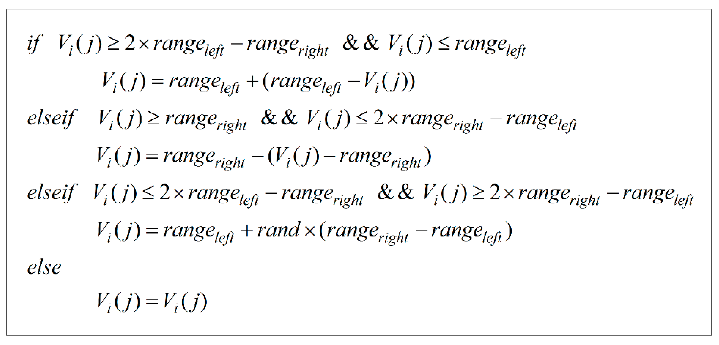
Step 6: Cross-border processing. The classical DE does not consider how to address the constraints handling. The randomness of the general cross-border processing strategy is too strong to preserve the historical optimal information accumulated through evolution. We used the symmetric mapping processing strategy as previously reported [31]. As shown in Figure 7, rangeleft and rangeright are the left and right boundaries of each variable in the individual, respectively. When the extent to which a variable violates the constraint is less than the absolute value of the variable range, the boundary point is taken as the center to map this variable equidistantly onto the range of value.
Step 7: Competitive survival operation. We used the idea of competition survival to compare the fitness and penalty function of the corresponding individual in the parent population and temporary population, and selected the preferable individual to form a new population. The specific rules are: (1) if both individuals do not violate the constraints, we judge them by comparing their fitness values; (2) if a solution satisfies the constraints, whereas the other one does not, then the solution meeting the constraints is better; and (3) if both do not meet the constraints, the solution with the lower penalty function is better.
Step 8: Evolution and iteration. We determined whether the scheduled iterations are reached. If so, then the operation is stopped; otherwise, proceed to step 3. If the desired iterations are reached, but the satisfactory solution has not been found, the population size and the iterations should be adjusted.
4. Multi-Objective Modeling and Solving
Many uncertainties exist in the weapons development process. One uncertainty is the development speed of military technology. Another uncertainty is the development process and conditions, such as funds, talents, and management [32]. These uncertainties result in risk during the development of weapons, meaning that the weapons may not attain the initially planned threat value. Therefore, DMs should consider the risk in weapons development so as to minimize the risk and meet future needs.
4.1. Development Risk Modeling
Weapons development risk refers to the possibility that weapons may not attain the tactical and technical index given the constraints imposed by limited resources, which negatively impacts the overall performance of combat [33]. Therefore, we first reasonably modelled the risk. In general, risk is defined as the consequence of failing to reach the expected purpose, multiplied by the probability of that consequence [34]. According to the typical risk model, which is called Expected Downside Risk (EDR) [35]:
where π is the target value, x is the actual value, and α is the risk sensitive exponent. The model considers the difference between the actual value and the target value as the consequence, and calculates the sum of the probability of all consequences. We used this model to define the gap between the actual threat reduction value and the expected value as the consequence, and then totaled all gaps with the corresponding probabilities to measure the risk.
Assuming that I possibilities of threat reduction value of each weapon exist, then the ith possible threat reduction value is:
where Ai is the conversion coefficient of the ith possible threat reduction value, T denotes the expected maximum value of the threat reduction without considering any constraints, and ηk denotes the risk sensitive coefficient of the expected maximum threat reduction value. The probability of T′ is modelled as:
where Pi is the probability conversion coefficient of the ith possible threat reduction value and t is the development duration of the weapon. For the weapons that can counter the same threat value, the longer is the development duration, the greater is the probability that the weapon will achieve the expected effect, and the smaller is the risk, and vice versa.
Based on the above model, the total weapons development risk of B is defined as:
4.2. Optimization Model
According to the threat gap planning model outlined in Section 3 and Equation (25), we built a multi-objective optimization model, which allows DMs to balance the two objectives of threat and risk, and obtains the best compromise solution to create a combined weapons planning scheme.
Therefore, the problem is treated as a typical Multi-Objective Optimization Problem (MOOP). The objectives that need to be optimized can be represented by an objective function set and certain equality or inequality constraints, and conflicts often exist among these objectives. It is impossible to simultaneously optimize all sub-objective functions; instead, we can obtain a compromise solution to these objectives, which is the Pareto optimality problem, first proposed by Pareto [36].
A global optimal solution to the single-objective optimization problem must exist. Conversely, it is possible that no definite optimal solution exists, but an acceptable solution set to MOOP may be possible. When all objectives are considered, the acceptable solution set is the best solution within the entire search space. However, the solution may not be optimal from the perspective of any of the sub-objectives. This solution set is called a Pareto optimal set, or non-dominated set, and the other solution set is called a dominated set. Because any of the solutions in the non-dominated set are not better than the other solutions, then the key to solve MOOP lies in how to find the Pareto optimal set, and determine the most appropriate solution in the Pareto optimal set according to the preference of the DMs.
4.2.1. Non-Dominated Sorting Differential Evolution Algorithm
The NSGA-II is a popular optimization method used to solve MOOP [37]. In 1994, NSGA was proposed by Srinivas and Deb [38]. Based on the shortcomings of NSGA, Deb et al. introduced NSGA-II in 2000 [39], which has gradually become the mainstream algorithm used for solving MOOP. It uses non-dominated sorting and shared variable methods to effectively maintain the diversity of Pareto frontiers. However, NSGA-II does not perform well in processing MOOP with a complex Pareto front. Given these shortcomings of NSGA-II, we designed an improved algorithm, which we have called the non-dominated sorting differential evolution (NSDE) algorithm. NSDE introduces a differential evolution operator to replace the crossover operation in NSGA-II and adaptively adds the global optimal solution information in the new generations to improve the local search accuracy and diversity. Considering the characteristics of the model, we combined NSGA-II with DE, and designed the following solving algorithm.
- Step 1
- Define the parameters of the algorithm. Define population size, iterations, and the crossover probability parameter, and the counter is set to 0.
- Step 2
- Initialize the population. The initial population is randomly generated and the individual encoding structure is outlined in Section 3.3.
- Step 3
- Sort the population. According to the objective function and constraints, evaluate the individuals. Use non-dominated sorting on the initial population to obtain the Pareto solution set. Then individuals are given ranks and crowding distance values. The binary tournament selection operation is implemented on the population.
- Step 4
- Mutation and crossover. The mutation operator based on DE was used to mutate the population. Simultaneously, a new population Q is obtained by using crossover operation on each of the individuals with a certain probability.
- Step 5
- Evaluate the temporary population. The temporary population is composed of the present population P and the offspring population Q, and non-dominated sorting of the temporary population is performed by comparing the rank and crowding distance of the individuals.
- Step 6
- Generate a new population. Select the best individuals from the temporary population to generate the new population.
- Step 7
- Evolution and iteration. If the number of iterations is reached, the Pareto optimal solution is output. Otherwise, the counter increases, and we continue back to Step 3.
4.2.2. Compromise Solution Based on TOPSIS
After obtaining the Pareto optimal set, evaluating the solution in the Pareto optimal set and selecting the compromise solution according to the preference of the DM are necessary. To date, many methods can be used to obtain a compromise solution from the Pareto optimal set. We used the classical TOPSIS method proposed by Hwang and Yoon [40] to obtain the compromise solution. TOPSIS essentially compares the proximity between different schemes and the ideal scheme. The main steps are as follows:
Step 1: Establish a decision matrix. Establish and normalize the decision matrix . p is the number of solutions, and 2 is the number of evaluation criteria, which, in this paper, are the threat gap and weapons development risk.
Step 2: Standardization the Decision matrix. Establish the weighted standardized decision matrix , where qj is the weight value of the jth criteria.
Step 3: Define the ideal solution. Define the positive ideal solution and the negative ideal solution . Because the threat gap and weapons development risk are both cost-type indexes:
Step 4: Calculate the Euclidean distance between each scheme and the positive and negative ideal solutions.
Step 5: Sort all solutions. Calculate the relative approach degree Ci between each scheme and the ideal point.
Finally, sort Ci in descending order. The solution with the largest Ci value is the optimal solution in the Pareto solution set.
5. Validation Demonstration
To clearly illustrate the application and procedure of the proposed approach and to demonstrate its feasibility and effectiveness, a case study is presented in this section.
5.1. Parameters Settings
Two countries, denoted as the attacker (R) and the defender (B), are in conflict with each other. R will deploy a sort of weapons in the next five years. As a result, B should develop a defense system consisting of new weapons as CMs.
As shown in Table 2, R1, R2, R3, R4, R5, R6, R7 and R8 are R’s current weapons; B1, B2, B3, B4, B5, B6, B7, B8, B9 and B10 are new weapons that B may develop. Each weapon can be characterized as one or several meta-functional nodes. For example, R1 is abstracted into two meta-functional nodes. B1 is abstracted into three meta-functional nodes. In addition to the functional descriptions of the nodes, the threat vectors that can counter R must be computed.
Part of the data is obtained from prior studies on [41,42]. Tactical and technical index values of B’s weapons are shown in Table 3.
The reference values of the tactical and technical indexes are provided in Table 4, and the normalization result is calculated in Table 5 according to the normalization method mentioned in Section 2.2.2.
Next, we classified and aggregated the threat value of various nodes. The result was shown in Table 6. The weights were set to be the same. To facilitate the calculation, we set all threats from R as 40.
Some restrictions exist based on real-life operational situations: (1) if more than one S node exists in one loop, they can only be arranged based on their values of Radius in descending order. For example, the Radius of SB3 and SB2 are 10 and 5, respectively. Then, SB3→SB2 is logical, SB2→SB3 is unreasonable; (2) if more than one D node exists in one loop, they can only be arranged in descending order in terms of Efficiency. For example, the Efficiency of DB2 and DB9 are 15 and 10, respectively. Then, DB2→DB9 is logical, DB9→DB2 is unreasonable; (3) for the connection from node S to node D, due to the limitation of communication links, DB1, DB2, DB3, and DB9 can only receive information from SB1, SB2, SB3, and SB9, respectively. SB5 and SB7 can only pass information to DB2. SB8 and SB10 can only pass information to DB9; (4) for node I, due to the limitation of communication links, IB1, IB2, and IB3 can only receive information from DB1, DB2, and DB3, respectively. IB4, IB6, and IB7 can only receive a strike command from DB2. IB10 can only receive a strike command from DB9; and (5) for the same functional nodes, more than two nodes cannot exist simultaneously in one loop. Based on the loops finding rules, a total of 115 loops covering the opponent nodes are found. The distribution of loops is shown in Table 7. The structure and threat values of all loops are shown in Table A1.
The related parameters of the weapons to be developed are shown in Table 8. The total budget is set as .
5.2. Numerical Results
Table 9 depicts the parameters used in this study associated with DE.
Herein, two other algorithms, Genetic Algorithm (GA) [43] and Particle Swarm Optimization (PSO) [44], were also applied independently under the same conditions. We ran the above three algorithms 10 times independently. Figure 8 shows the best evolutionary curves corresponding to the three algorithms, obtained with the evolutionary generations of the algorithm as abscissa and the optimization objective function DB in Equation (26) as the ordinate. The smaller is the threat gap, the better is the corresponding planning. In particular, the final objective function values obtained by DE and PSO are considerably better than that of GA. Comparing DE with PSO, although the two final objective function values are basically the same, DE converges to a satisfactory solution at a faster rate, in about 60 generations, whereas PSO required about 280 generations. The minimum DE threat gap is 20.6594 with the best individual as [4, 1, 1, 2, 3, 1, 1, 5, 1, 1, 21, 8, 14, 7, 27, 6, 28, 38, 33, 40].
We statistically analyzed the results, as shown in Table 10. The optimal value, the worst value, the mean value, the middle value, and the variance of the function in the 10 running results were tabulated. The optimal and worst value illustrate the merits of the scheme. The average value reflects the overall quality of the algorithm. The mid-value explains the convergence speed of the algorithm, to a certain extent. The variance is the overall stability of the algorithm.
All DE indexes are better than those of GA and PSO. Although the optimal solution found by PSO is close to the optimal solution calculated by DE, the mid-value and variance corresponding to the PSO result are inferior to those of DE. In summary, DE has better efficiency and stability for this model.
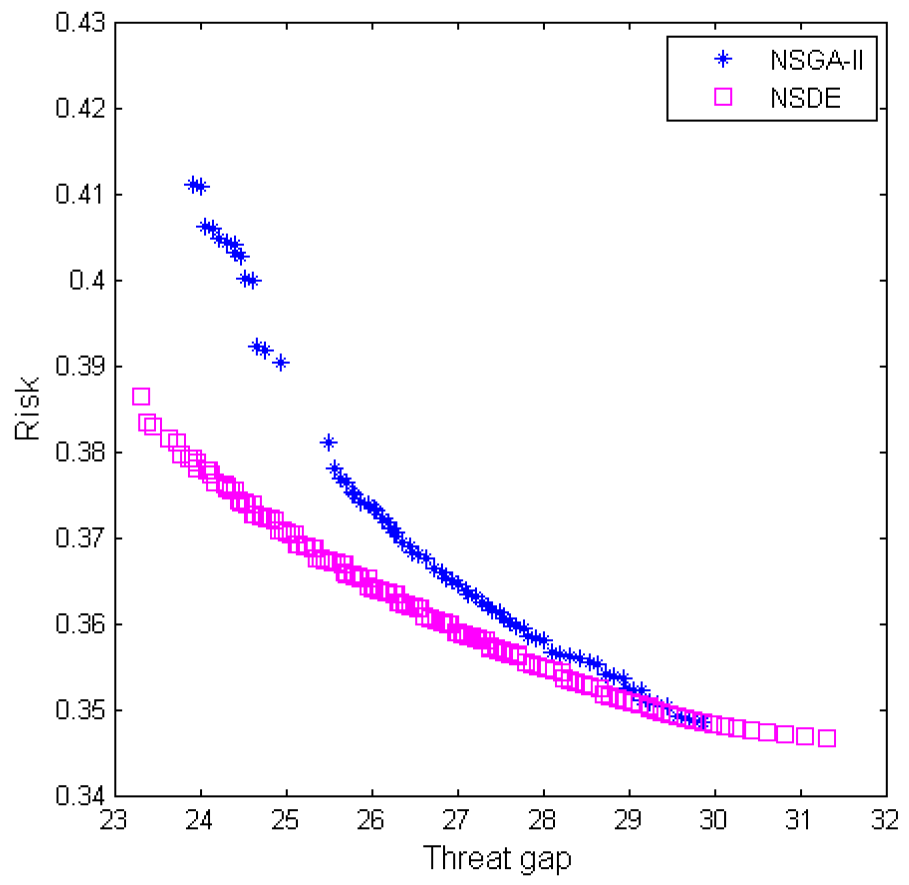
As for multi-objective optimization, NSDE and NSGA-II were used to optimize the weapons development scheme to obtain the Pareto optimal set, and then the TOPSIS method was used to find the compromise solution. Similarly, we ran the two algorithms 10 times independently. Each algorithm obtained 10 Pareto sets. Then, these solutions were sorted. The best solutions were selected to form the Pareto solution set of the two algorithms, as shown in Figure 9, which is plotted with the optimization objective function RB in Equation (26) as the ordinate, against the optimization objective function DB in Equation (26) as the abscissa. The coordinate axis is the same in Figure 10.
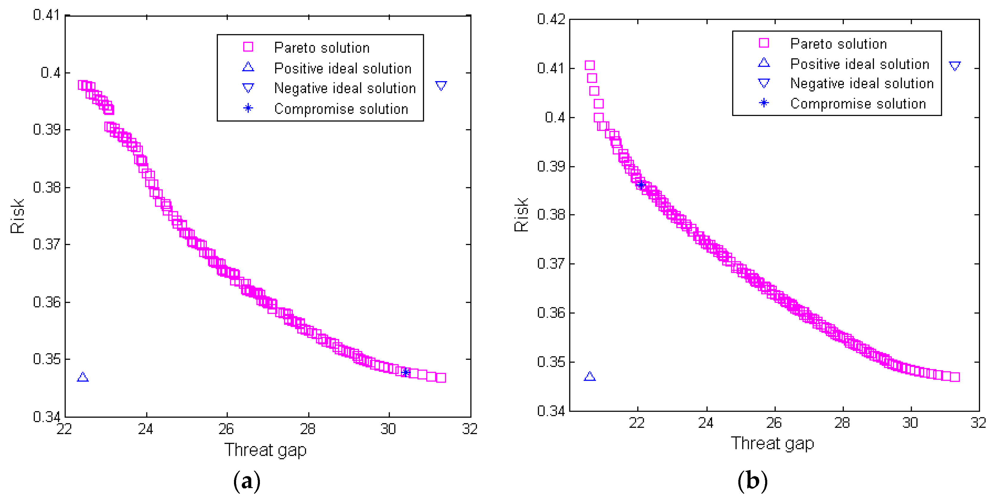
NSDE has a longer evolutionary curve than the traditional NSGA-II. Comparing the results of the two algorithms, the NSDE Pareto solutions are superior to those of NSGA-II in terms of diversity and convergence. We set the weighted values of the threat gap and the risk objectives as 0.6 and 0.4, respectively. The compromise solution calculated by the TOPSIS method is shown in Figure 10, which is [1, 1, 1, 1, 1, 1, 1, 5, 5, 1, 8, 7, 12, 6, 23, 5, 26, 30, 21, 40].
Uncertainty exists in the weapons R&D process and in all model relationships. A sensitivity analysis was performed for certain variables to examine the uncertainties of the model. Herein, the total budget was set as 200 and 230. The compromise solutions calculated by NSDE and TOPSIS are shown in Figure 11, which are [1, 1, 1, 1, 1, 1, 1, 5, 1, 5, 8, 7, 12, 6, 19, 5, 21, 30, 21, 32] and [1, 1, 1, 1, 1, 1, 1, 5, 1, 1, 8, 7, 12, 6, 21, 5, 24, 30, 27, 40]. Compared to the original settings, the maximum difference between these programs is related to the ninth and tenth weapons. The model is affected less by uncertainty. The results indicate that their R&D risks may be high. In the development process of these two weapons, DMs should focus on the technical progress and upgrading to reduce risk.
5.3. Results Analysis
In this section, we analyze the model based on the numerical results.
5.3.1. Comparison of a Single Objective and Multi-Objective
The best planning solution of the single objective problem is [4, 1, 1, 2, 3, 1, 1, 5, 1, 1, 21, 8, 14, 7, 27, 6, 28, 38, 33, 40], and the compromise solution of the multi-objective problem is [1, 1, 1, 1, 1, 1, 1, 5, 5, 1, 8, 7, 12, 6, 23, 5, 26, 30, 21, 40]. As for the investment, the maximum difference between these two results is related to the first and eighth weapons, which means that their threat reduction effects are the best operation loops to counter the enemy. DMs can focus on developing these two weapons by increasing the amount of investment or reducing uncertain risks. As for time, the difference between these two results is related to the first and ninth weapons, indicating that their R&D risks are very high. In the development process of these two weapons, DMs should ensure the risks are controlled.
5.3.2. Different Weights of Multi-Objective
Different DMs may have different preferences for the above-mentioned two objectives. Consequently, we used different weighted values for the threat gap and the risk objectives. The optimal results are shown in Table 11. If the DMs are risk-seeking, they can set the weight of the development risk objective lower. On the contrary, if the DMs are risk-averse, they can set the weight of the development risk objective higher. We also found that the risk value does not increase even when the DM is generally displaying a risk-seeking tendency when making choices.
5.3.3. Decision Preference
During the actual decision-making process, DMs must artificially adjust and optimize the planning to coordinate the development of weapons. Consider a scenario with an m-period and M weapons to be developed: (1) if the ith weapon must be developed in the jth year, then, the time encoding of the ith weapon is set to j when initializing the population; and (2) if the development duration of the ith weapon must satisfy k years, then, the investment encoding of the ith weapon is set to a/k when initializing the population. The logic is applied when other similar situations occur. The model and the corresponding solving algorithm allow users to set specific encoding and adjust the development planning based on individual preferences. The model is practical for actual application.
6. Conclusions
This paper proposed a new approach to solve the problem of allocating limited resources when developing military CMs versus probabilistic threat, with emphasis on representing the cooperation relationships among different weapons. The competition between hostile countries was transformed into an operation loop-based optimization model. We applied the system dynamics principle to characterize the dynamic behavior of the nodes in a complex weapons network. The intrinsic properties of a weapon were converted into certain constraints. To address the development of CMs with limited resources to counter the enemy, the threat gap was set as the single objective function. In addition, considering the uncertainties in the development process, the R&D risks of weapons were used to optimize the planning. Ultimately, certain intelligent optimization algorithms were used to obtain a numerical solution.
The numerical results showed that more investments result in a more effective design, and more time leads to lower risk. The key weapons that can effectively reduce threat and could potentially encounter technical difficulties during R&D should be developed as soon as possible. With a fixed investment amount, the results also demonstrate that the system effectiveness can be significantly improved by increasing the amount allocated to the weapon that is found in more operation loops.
Future research directions include allowing for uncertainty in players’ preferences, having a dynamic resource distribution strategy over a certain time horizon, and enabling multiple players or multi-objective in a sequential game. These challenges will contribute to the expansion of this methodology for tackling a broader range of problems.
Acknowledgments
The study was supported partially by the National Natural Science Foundation of China under Grant Nos. 71690233, 71501182, and 71571185.
Author Contributions
Kewei Yang and Chunqi Wan conceived the study. Chunqi Wan and Xiaoxiong Zhang designed the optimization model. Qingsong Zhao designed the experiments and validated the model. Chunqi Wan wrote the draft. All authors gave critical revisions and approved the submission.
Conflicts of Interest
The authors declare no conflict of interest.
Appendix A

Table A1.
Parameters of loops.
| Node Sequence | Node Sequence | ||
|---|---|---|---|
| T→SB1→DB1→IB1→T | 0.266175 | T→SB7→SB2→DB2→IB2→T | 0.176472 |
| T→SB2→DB2→IB2→T | 0.1539 | T→SB7→SB2→DB2→IB4→T | 0.188856 |
| T→SB2→DB2→IB4→T | 0.110565 | T→SB7→SB2→DB2→IB6→T | 0.117648 |
| T→SB2→DB2→IB6→T | 0.100035 | T→SB7→SB2→DB2→IB7→T | 0.1548 |
| T→SB2→DB2→IB7→T | 0.071867 | T→SB10→SB1→DB1→IB1→T | 0.095086 |
| T→SB3→DB3→IB3→T | 0.23324 | T→SB10→SB2→DB2→IB2→T | 0.077369 |
| T→SB5→DB2→IB2→T | 0.089964 | T→SB10→SB2→DB2→IB4→T | 0.091564 |
| T→SB5→DB2→IB4→T | 0.186323 | T→SB10→SB2→DB2→IB6→T | 0.074504 |
| T→SB5→DB2→IB6→T | 0.10773 | T→SB10→SB2→DB2→IB7→T | 0.126781 |
| T→SB5→DB2→IB7→T | 0.058477 | T→SB9→SB1→DB1→IB1→T | 0.103159 |
| T→SB7→DB2→IB2→T | 0.077396 | T→SB9→SB2→DB2→IB2→T | 0.204955 |
| T→SB7→DB2→IB4→T | 0.062975 | T→SB9→SB2→DB2→IB4→T | 0.118503 |
| T→SB7→DB2→IB6→T | 0.1647 | T→SB9→SB2→DB2→IB6→T | 0.126819 |
| T→SB7→DB2→IB7→T | 0.107055 | T→SB9→SB2→DB2→IB7→T | 0.079002 |
| T→SB8→DB9→IB10→T | 0.11529 | T→SB9→SB3→DB3→IB3→T | 0.10395 |
| T→SB9→DB9→IB10→T | 0.1482 | T→SB9→SB5→DB2→IB2→T | 0.179595 |
| T→SB10→DB9→IB10→T | 0.1586 | T→SB9→SB5→DB2→IB4→T | 0.114114 |
| T→SB2→DB2→DB1→IB1→T | 0.10647 | T→SB9→SB5→DB2→IB6→T | 0.122122 |
| T→SB2→DB2→DB3→IB3→T | 0.086632 | T→SB9→SB5→DB2→IB7→T | 0.076076 |
| T→SB2→DB2→DB9→IB10→T | 0.138411 | T→SB9→SB7→DB2→IB2→T | 0.1001 |
| T→SB5→DB2→DB1→IB1→T | 0.080028 | T→SB9→SB7→DB2→IB4→T | 0.158004 |
| T→SB5→DB2→DB3→IB3→T | 0.085644 | T→SB9→SB7→DB2→IB6→T | 0.169092 |
| T→SB5→DB2→DB9→IB10→T | 0.121285 | T→SB9→SB7→DB2→IB7→T | 0.105336 |
| T→SB7→DB2→DB1→IB1→T | 0.057494 | T→SB9→SB10→DB9→IB10→T | 0.1386 |
| T→SB7→DB2→DB3→IB3→T | 0.046781 | T→SB8→SB2→DB2→DB1→IB1→T | 0.085135 |
| T→SB7→DB2→DB9→IB10→T | 0.1026 | T→SB8→SB2→DB2→DB3→IB3→T | 0.069272 |
| T→SB8→SB1→DB1→IB1→T | 0.0988 | T→SB8→SB2→DB2→DB9→IB10→T | 0.081982 |
| T→SB8→SB2→DB2→IB2→T | 0.06669 | T→SB8→SB5→DB2→DB1→IB1→T | 0.066707 |
| T→SB8→SB2→DB2→IB4→T | 0.07182 | T→SB8→SB5→DB2→DB3→IB3→T | 0.113513 |
| T→SB8→SB2→DB2→IB6→T | 0.053352 | T→SB8→SB5→DB2→DB9→IB10→T | 0.092363 |
| T→SB8→SB2→DB2→IB7→T | 0.135 | T→SB8→SB7→DB2→DB1→IB1→T | 0.43043 |
| T→SB8→SB3→DB3→IB3→T | 0.13 | T→SB8→SB7→DB2→DB3→IB3→T | 0.385385 |
| T→SB8→SB5→DB2→IB2→T | 0.2052 | T→SB8→SB7→DB2→DB9→IB10→T | 0.335335 |
| T→SB8→SB5→DB2→IB4→T | 0.2196 | T→SB1→SB2→DB2→DB1→IB1→T | 0.135135 |
| T→SB8→SB5→DB2→IB6→T | 0.1368 | T→SB1→SB2→DB2→DB3→IB3→T | 0.13013 |
| T→SB8→SB5→DB2→IB7→T | 0.18 | T→SB1→SB2→DB2→DB9→IB10→T | 0.18018 |
| T→SB8→SB7→DB2→IB2→T | 0.14742 | T→SB3→SB2→DB2→DB1→IB1→T | 0.331431 |
| T→SB8→SB7→DB2→IB4→T | 0.119952 | T→SB3→SB2→DB2→DB3→IB3→T | 0.288388 |
| T→SB8→SB7→DB2→IB6→T | 0.08775 | T→SB3→SB2→DB2→DB9→IB10→T | 0.178337 |
| T→SB8→SB7→DB2→IB7→T | 0.0945 | T→SB5→SB2→DB2→DB1→IB1→T | 0.103113 |
| T→SB8→SB9→DB9→IB10→T | 0.0702 | T→SB5→SB2→DB2→DB3→IB3→T | 0.110349 |
| T→SB8→SB10→DB9→IB10→T | 0.191646 | T→SB5→SB2→DB2→DB9→IB10→T | 0.068742 |
| T→SB1→SB2→DB2→IB2→T | 0.110808 | T→SB7→SB2→DB2→DB1→IB1→T | 0.09045 |
| T→SB1→SB2→DB2→IB4→T | 0.118584 | T→SB7→SB2→DB2→DB3→IB3→T | 0.258208 |
| T→SB1→SB2→DB2→IB6→T | 0.073872 | T→SB7→SB2→DB2→DB9→IB10→T | 0.116216 |
| T→SB1→SB2→DB2→IB7→T | 0.0972 | T→SB10→SB2→DB2→DB1→IB1→T | 0.111912 |
| T→SB3→SB1→DB1→IB1→T | 0.079607 | T→SB10→SB2→DB2→DB3→IB3→T | 0.154955 |
| T→SB3→SB2→DB2→IB2→T | 0.064774 | T→SB10→SB2→DB2→DB9→IB10→T | 0.087838 |
| T→SB3→SB2→DB2→IB4→T | 0.228911 | T→SB9→SB2→DB2→DB1→IB1→T | 0.094595 |
| T→SB3→SB2→DB2→IB6→T | 0.132354 | T→SB9→SB2→DB2→DB3→IB3→T | 0.07027 |
| T→SB3→SB2→DB2→IB7→T | 0.141642 | T→SB9→SB2→DB2→DB9→IB10→T | 0.097297 |
| T→SB5→SB1→DB1→IB1→T | 0.088236 | T→SB9→SB5→DB2→DB1→IB1→T | 0.074079 |
| T→SB5→SB2→DB2→IB2→T | 0.1161 | T→SB9→SB5→DB2→DB3→IB3→T | 0.060276 |
| T→SB5→SB2→DB2→IB4→T | 0.200586 | T→SB9→SB5→DB2→DB9→IB10→T | 0.09054 |
| T→SB5→SB2→DB2→IB6→T | 0.127452 | T→SB9→SB7→DB2→DB1→IB1→T | 0.104054 |
| T→SB5→SB2→DB2→IB7→T | 0.136396 | T→SB9→SB7→DB2→DB3→IB3→T | 0.1002 |
| T→SB5→SB3→DB3→IB3→T | 0.084968 | T→SB9→SB7→DB2→DB9→IB10→T | 0.138739 |
| T→SB7→SB1→DB1→IB1→T | 0.1118 |
References
- Golany, B.; Goldberg, N.; Rothblum, U.G. Allocating multiple defensive resources in a zero-sum game setting. Ann. Oper. Res. 2015, 225, 91–109. [Google Scholar] [CrossRef]
- Bier, V.M.; Haphuriwat, N.; Menoyo, J.; Zimmerman, R.; Culpen, A.M. Optimal resource allocation for defense of targets based on differing measures of attractiveness. Risk Anal. 2008, 28, 763–770. [Google Scholar] [CrossRef] [PubMed]
- Etcheson, C. Arms Race Theory: Strategy and Structure of Behavior; Greenwood Press: New York, NY, USA, 1989; Volume 6. [Google Scholar]
- Gu, L.; Wang, S.; Zhao, F. Weapon system of systems capability planning model based on expected effectiveness. Syst. Eng. Electron. 2017, 39, 329–334. [Google Scholar]
- Håkenstad, M.; Larsen, K.K. Long-Term Defence Planning: A Comparative Study of Seven Countries; Institutt for Forsvarsstudier: Oslo, Norway, 2012. [Google Scholar]
- Zhang, X.; Ge, B.; Jiang, J.; Tan, Y. Capability requirements oriented weapons portfolio planning model and algorithm. J. Natl. Univ. Def. Technol. 2017, 39, 102–108. [Google Scholar]
- Golany, B.; Kress, M.; Penn, M.; Rothblum, U.G. Resource allocation in a technology race with temporary advantages. Nav. Res. Logist. 2012, 59, 128–145. [Google Scholar] [CrossRef] [Green Version]
- Richardson, L.F. Mathematical psychology of war. Nature 1935, 136, 1025. [Google Scholar] [CrossRef]
- Hunter, J.E. Mathematical models of a three-nation arms race. J. Confl. Resolut. 1980, 24, 241–252. [Google Scholar] [CrossRef]
- Paulson, E.C.; Linkov, I.; Keisler, J.M. A game theoretic model for resource allocation among countermeasures with multiple attributes. Eur. J. Oper. Res. 2016, 252, 610–622. [Google Scholar] [CrossRef]
- Golany, B.; Goldberg, N.; Rothblum, U.G. A two-resource allocation algorithm with an application to large-scale zero-sum defensive games. Comput. Oper. Res. 2016, 78, 218–229. [Google Scholar] [CrossRef]
- Mazicioglu, D.; Merrick, J.R.W. Behavioral modeling of adversaries with multiple objectives in counterterrorism. Risk Anal. 2017. [Google Scholar] [CrossRef] [PubMed]
- Wan, C.; Xiong, W.; Ye, Y.; Zhao, Q.; Yang, K. Research on development strategy of weapon equipment in antagonistic environment. In Proceedings of the 2017 Annual IEEE Systems Conference (Syscon), Montreal, QC, Canada, 24–27 April 2017. [Google Scholar]
- Deller, S.; Bell, M.I.; Bowling, S.R.; Rabadi, G.A.; Tolk, A. Applying the information age combat model: Quantitative analysis of network centric operations. Int. C2 J. 2009, 3, 1–25. [Google Scholar]
- Golany, B.; Kress, M.; Penn, M.; Rothblum, U.G. Network optimization models for resource allocation in developing military counter measures. Oper. Res. 2012, 60, 48–63. [Google Scholar] [CrossRef] [Green Version]
- Shih, C.; Koong, C.S.; Hsiung, P.A. Billiard combat modeling and simulation based on optimal cue placement control and strategic planning. J. Intell. Robot. Syst. 2012, 67, 25–41. [Google Scholar] [CrossRef]
- Li, J.; Tan, Y.; Yang, K.; Zhang, X.; Ge, B. Structural robustness of combat networks of weapon system-of-systems based on the operation loop. Int. J. Syst. Sci. 2017, 48, 659–674. [Google Scholar] [CrossRef]
- Sun, J.; Ge, B.; Li, J.; Yang, K. Operation network modeling with degenerate causal strengths for missile defense systems. IEEE Syst. J. 2016, 99, 1–11. [Google Scholar] [CrossRef]
- Cares, J. Distributed Networked Operations: The Foundations of Network Centric Warfare; iUniverse: Bloomington, IN, USA, 2006. [Google Scholar]
- Brehmer, B. The dynamic OODA loop: Amalgamating boyd’s ooda loop and the cybernetic approach to command and control. In Proceedings of the 10th International Command & Control Research & Technology Symposium (ICCRTS), McLean, VA, USA, 13–16 June 2005. [Google Scholar]
- Tan, Y.J.; Zhang, X.K.; Yang, K.W. Research on networked description and modeling methods of armament system-of-systems. J. Syst. Manag. 2012, 21, 781–786. [Google Scholar]
- Zhao, D.; Dou, Y.; Zhao, Q.; Zhan, W. The method to evaluate the command and control effectiveness of operational system under uncertain threat situation. In Proceedings of the 2016 Chinese Control and Decision Conference (CCDC), Yinchuan, China, 28–30 May 2016. [Google Scholar]
- Zuo, X.; Qu, Y. Operational ability evaluation model of the armored weapon system of system. In Proceedings of the 2013 25th Chinese Control and Decision Conference (CCDC), Guiyang, China, 25–27 May 2013. [Google Scholar]
- Danling, Z.; Yuejin, T.; Jichao, L. Armament system of systems contribution evaluation based on operation loop. Syst. Eng. Electron. 2017, 39, 2239–2247. [Google Scholar]
- Guo, X.; Li, J. A new synchronization algorithm for delayed complex dynamical networks via adaptive control approach. Commun. Nonlinear Sci. Numer. Simul. 2012, 17, 4395–4403. [Google Scholar] [CrossRef]
- Storn, R.; Price, K. Differential evolution—A simple and efficient heuristic for global optimization over continuous spaces. J. Glob. Optim. 1997, 11, 341–359. [Google Scholar] [CrossRef]
- Nobakhti, A.; Wang, H. A simple self-adaptive differential evolution algorithm with application on the alstom gasifier. Appl. Soft Comput. J. 2008, 8, 350–370. [Google Scholar] [CrossRef]
- Michalewicz, Z.; Schoenauer, M. Evolutionary algorithms for constrained parameter optimization problems. Evol. Comput. 1996, 4, 1–32. [Google Scholar] [CrossRef]
- Coello, C.A.C. Theoretical and numerical constraint-handling techniques used with evolutionary algorithms: A survey of the state of the art. Comput. Methods Appl. Mech. Eng. 2002, 191, 1245–1287. [Google Scholar] [CrossRef]
- Price, K.; Storn, R.M.; Lampinen, J.A. Differential Evolution: A Practical Approach to Global Optimization; Natural Computing Series; Springer: New York, NY, USA, 2005; pp. 1–24. [Google Scholar]
- Zhou, Y.; Jiang, J.; Yang, Z.; Tan, Y. A hybrid approach for multi-weapon production planning with large-dimensional multi-objective in defence manufacturing. Proc. Inst. Mech. Eng. Part B J. Eng. Manuf. 2014, 228, 302–316. [Google Scholar] [CrossRef]
- Brown, M.M. Acquisition Risks in a World of Joint Capabilities; Proceedings Paper; Naval Postgraduate School: Monterey, CA, USA, 2011. [Google Scholar]
- Xu, Z.; Wu, J.J. Status quo and prospect of research on technical risk for weapon system development. J. Beijing Univ. Aeronaut. Astronaut. 2008, 21, 6–9. [Google Scholar]
- Mun, J. Modeling Risk; John Wiley & Sons Inc.: Hoboken, NJ, USA, 2006. [Google Scholar]
- Fishburn, P.C. Mean-risk analysis with risk associated with below-target returns. Am. Econ. Rev. 2001, 67, 116–126. [Google Scholar]
- Pareto, V. Cours d’Economies Politique; F Rouge: Lausanne, Switzerland, 1896; Volume I and II. [Google Scholar]
- Horta, N.; Rui, N.; Correia, M. A multi-objective routing algorithm for wireless multimedia sensor networks. Appl. Soft Comput. 2015, 30, 104–112. [Google Scholar] [CrossRef]
- Srinivas, N.; Deb, K. Multiobjective optimization using nondominated sorting in genetic algorithms. Evol. Comput. 1994, 2, 221–248. [Google Scholar] [CrossRef]
- Deb, K.; Agrawal, S.; Pratap, A.; Meyarivan, T. A fast elitist non-dominated sorting genetic algorithm for multi-objective optimization: NSGA-II. In Proceedings of the International Conference on Parallel Problem Solving From Nature, Paris, Prance, 18–20 September 2000; pp. 849–858. [Google Scholar]
- Baykasoğlu, A.; Gölcük, İ. Development of a novel multiple-attribute decision making model via fuzzy cognitive maps and hierarchical fuzzy topsis. Inf. Sci. 2015, 301, 75–98. [Google Scholar] [CrossRef]
- Ren, X.G. Foreign tank armored vehicle active protection system imtroduction. Fire Control Command Control 2010, 35, 4–6. [Google Scholar]
- Yang, C.C.; Yang, M.H. Constraint networks: A survey. In Proceedings of the IEEE International Conference on Systems, Man, and Cybernetics. Computational Cybernetics and Simulation, Orlando, FL, USA, 12–15 October 1997; Volume 1932, pp. 1930–1935. [Google Scholar]
- Kuo, C.C.; Liu, C.H.; Chang, H.C.; Lin, K.J. Implementation of a motor diagnosis system for rotor failure using genetic algorithm and fuzzy classification. Appl. Sci. 2017, 7, 31. [Google Scholar] [CrossRef]
- Liang, C.; Tong, X.; Lei, T.; Li, Z.; Wu, G. Optimal design of an air-to-air heat exchanger with cross-corrugated triangular ducts by using a particle swarm optimization algorithm. Appl. Sci. 2017, 7, 554. [Google Scholar] [CrossRef]
Figure 1.
(a) Threat mitigation; and (b) threat accumulation.
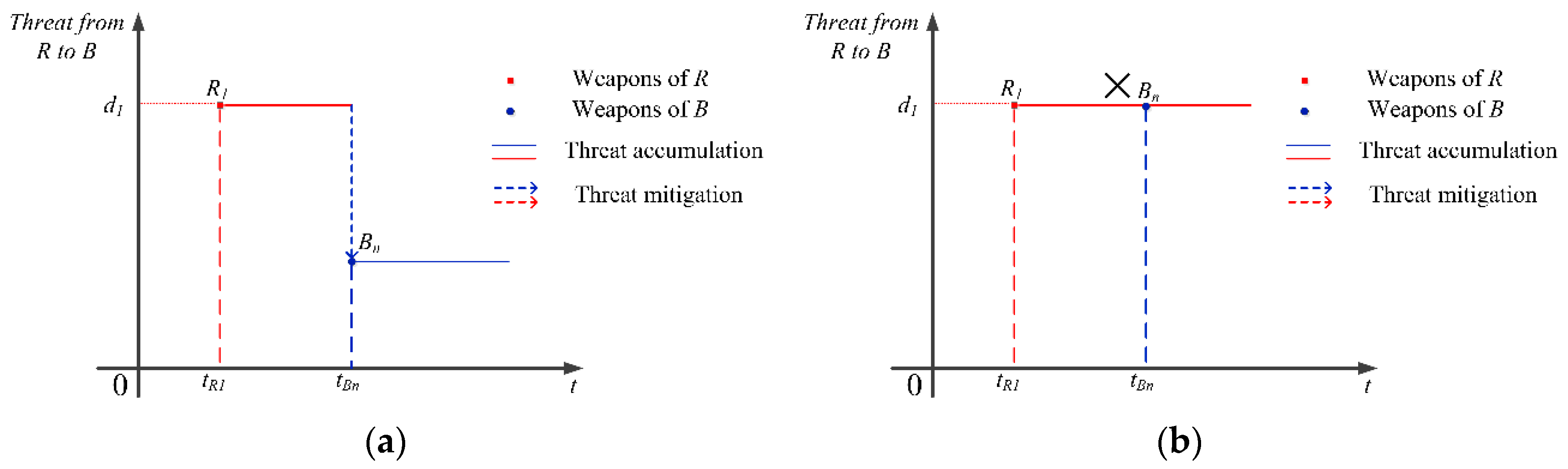
Figure 2.
Weapon system of systems nodes location in battle.
Figure 3.
Schematic of an operation loop in battle.

Figure 4.
Threat accumulation over time.

Figure 5.
Relationship modeling between time and investment.
Figure 6.
Variable encoding.
Figure 7.
Symmetric mapping processing strategy.

Figure 8.
Results of the three algorithms.
Figure 9.
Pareto sets of two different algorithms.

Figure 10.
Compromise solution of the Pareto set.
Figure 11.
(a) Compromise solution with a total budget of 200; and (b) compromise solution with a total budget of 230.
Figure 11.
(a) Compromise solution with a total budget of 200; and (b) compromise solution with a total budget of 230.

Table 1.
Meta-functional edge relation types.
| Nodes | SR | DR | IR | SB | DB | IB |
|---|---|---|---|---|---|---|
| SR | SR→SR | SR→DR | SR→SB | |||
| DR | DR→SR | DR→DR | DR→IR | DR→SB | ||
| IR | IR→SB | IR→DB | IR→IB | |||
| SB | SB→SR | SB→SB | SB→DB | |||
| DB | DB→SR | DB→SB | DB→DB | DB→IB | ||
| IB | IB→SR | IB→DR | IB→IR |
Table 2.
WSOS composition.
| R | B | ||
|---|---|---|---|
| Name | Nodes | Name | Nodes |
| R1 | SR1, DR1 | R1 (Main Battle Tank) | SR1, DR1, IB1 |
| R2 | DR2, IR2 | R2 (Infantry Fighting Vehicle) | SB2, DB2, IB2 |
| R3 | IR3 | B3 (Armored Front Observation Command Vehicle) | SB3, DB3, IB3 |
| R4 | SB4, DR4, IR4 | B4 (Self-propelled Howitzer) | IB4 |
| R5 | SB5, IR5 | B5 (Low Level Search and Warning Radar Vehicle) | SB5 |
| R6 | SB6, DR6, IR6 | B6 (Self-propelled Antiaircraft Gun) | IB6 |
| R7 | SB7, IR7 | B7 (Armored Reconnaissance Vehicle) | SB7, IB7 |
| R8 | SB8, DR8 | B8 (Unmanned Aerial Vehicle) | SB8 |
| B9 (Reconnaissance Information Vehicle) | SB9, DB9 | ||
| B10 (Reconnaissance Attack Helicopter) | SB10, IB10 | ||
Table 3.
Tactical and technical index values.
| Weapon | S | D | I | |||||||||
|---|---|---|---|---|---|---|---|---|---|---|---|---|
| TS1 | TS2 | TS3 | TS4 | TD1 | TD2 | TD3 | TD4 | TI1 | TI2 | TI3 | TI4 | |
| B1 | 7 | 0.85 | 0.4 | 0.9 | 0.8 | 10 | 3 | 250 | 600 | 0.9 | 2 | 60 |
| B2 | 5 | 0.8 | 0.5 | 0.7 | 0.7 | 15 | 4 | 280 | 600 | 0.8 | 1.5 | 45 |
| B3 | 10 | 0.9 | 0.3 | 0.8 | 0.9 | 10 | 3 | 200 | 500 | 0.8 | 1 | 40 |
| B4 | - | - | - | - | - | - | - | - | 500 | 0.8 | 2.5 | 40 |
| B5 | 12 | 0.9 | 0.3 | 0.9 | - | - | - | - | - | - | - | - |
| B6 | - | - | - | - | - | - | - | - | 500 | 0.2 | 1.5 | 40 |
| B7 | 10 | 0.9 | 0.3 | 0.9 | - | - | - | - | 500 | 0.8 | 1 | 50 |
| B8 | 20 | 0.95 | 0.2 | 0.9 | - | - | - | - | - | - | - | - |
| B9 | 15 | 0.9 | 0.3 | 0.9 | 0.8 | 10 | 3 | 200 | - | - | - | - |
| B10 | 10 | 0.9 | 0.5 | 0.9 | - | - | - | - | 700 | 0.95 | 1.5 | 150 |
Table 4.
The reference values of the tactical and technical indexes.
| Node | Index | Unit | Max | Min |
|---|---|---|---|---|
| S | Radius (TS1) | km | 25 | 0 |
| Accuracy (TS2) | m | 1 | 0.1 | |
| DeteRate (TS3) | % | 1 | 0 | |
| HavestRate (TS4) | % | 1 | 0 | |
| D | CoverRate (TD1) | % | 800 | 0 |
| Efficiency (TD2) | Sec | 1 | 0 | |
| Community (TD3) | Sec | 3 | 0 | |
| Dlay (TD4) | Sec | 200 | 0 | |
| I | Radius (TI1) | km | 1 | 0 |
| Accuracy (TI2) | % | 20 | 0 | |
| RPG (TI3) | ton | 10 | 0 | |
| Mobility (TI4) | km/h | 500 | 0 |
Table 5.
Tactical and technical index normalization.
| Weapon | S | D | I | |||||||||
|---|---|---|---|---|---|---|---|---|---|---|---|---|
| TS1 | TS2 | TS3 | TS4 | TD1 | TD2 | TD3 | TD4 | TI1 | TI2 | TI3 | TI4 | |
| B1 | 0.28 | 0.83 | 0.60 | 0.90 | 0.80 | 0.50 | 0.70 | 0.50 | 0.75 | 0.90 | 0.67 | 0.30 |
| B2 | 0.20 | 0.78 | 0.50 | 0.70 | 0.70 | 0.25 | 0.60 | 0.44 | 0.75 | 0.80 | 0.50 | 0.23 |
| B3 | 0.40 | 0.89 | 0.70 | 0.80 | 0.90 | 0.50 | 0.70 | 0.60 | 0.63 | 0.80 | 0.33 | 0.20 |
| B4 | - | - | - | - | - | - | - | - | 0.63 | 0.80 | 0.83 | 0.20 |
| B5 | 0.48 | 0.89 | 0.70 | 0.90 | - | - | - | - | - | - | - | - |
| B6 | - | - | - | - | - | - | - | - | 0.63 | 0.20 | 0.50 | 0.20 |
| B7 | 0.40 | 0.89 | 0.70 | 0.90 | - | - | - | - | 0.63 | 0.80 | 0.33 | 0.25 |
| B8 | 0.80 | 0.94 | 0.80 | 0.90 | - | - | - | - | - | - | - | - |
| B9 | 0.60 | 0.89 | 0.70 | 0.90 | 0.80 | 0.50 | 0.70 | 0.60 | - | - | - | - |
| B10 | 0.40 | 0.89 | 0.50 | 0.90 | - | - | - | - | 0.88 | 0.95 | 0.50 | 0.75 |
Table 6.
Threat vector aggregation of nodes.
| Weapon | S | D | T |
|---|---|---|---|
| B1 | 0.65 | 0.63 | 0.65 |
| B2 | 0.54 | 0.50 | 0.57 |
| B3 | 0.70 | 0.68 | 0.49 |
| B4 | - | - | 0.61 |
| B5 | 0.52 | - | - |
| B6 | - | - | 0.38 |
| B7 | 0.72 | - | 0.50 |
| B8 | 0.86 | - | - |
| B9 | 0.77 | 0.65 | - |
| B10 | 0.67 | - | 0.77 |
Table 7.
Loops distribution.
| Node Number | Loop Number |
|---|---|
| 4 | 17 |
| 5 | 65 |
| 6 | 33 |
Table 8.
Parameters of the weapons.
| Weapon | cmin | cmax | tmin | tmax | aj |
|---|---|---|---|---|---|
| B1 | 8 | 24 | 1 | 3 | 24 |
| B2 | 7 | 14 | 1 | 2 | 14 |
| B3 | 12 | 18 | 2 | 3 | 36 |
| B4 | 6 | 12 | 1 | 2 | 12 |
| B5 | 15 | 30 | 2 | 4 | 60 |
| B6 | 5 | 15 | 1 | 3 | 15 |
| B7 | 21 | 28 | 3 | 4 | 84 |
| B8 | 30 | 50 | 3 | 5 | 150 |
| B9 | 21 | 35 | 3 | 5 | 105 |
| B10 | 32 | 40 | 4 | 5 | 160 |
Table 9.
DE parameters.
| Parameter | F | CR | NP | G |
|---|---|---|---|---|
| Value | 0.5 | 0.2 | 200 | 500 |
Table 10.
Comparison of algorithm results.
| Algorithm | DE | GA | PSO |
|---|---|---|---|
| Optimal | 20.6594 | 25.4480 | 21.1367 |
| Worst | 21.3432 | 26.7483 | 24.4506 |
| Mean | 21.0385 | 26.0738 | 22.0119 |
| Mid | 21.0617 | 26.1466 | 21.7246 |
| Variance | 0.0442 | 0.1945 | 1.0718 |
Table 11.
Comparison of algorithm results.
| Threat Gap Weight | Risk Weight | Threat Gap | Risk |
|---|---|---|---|
| 0.1 | 0.9 | 29.4559 | 0.3496 |
| 0.2 | 0.8 | 28.2249 | 0.3538 |
| 0.3 | 0.7 | 25.9497 | 0.3644 |
| 0.4 | 0.6 | 24.6378 | 0.3727 |
| 0.5 | 0.5 | 23.9671 | 0.3782 |
| 0.6 | 0.4 | 23.7865 | 0.3799 |
| 0.7 | 0.3 | 23.3864 | 0.3834 |
| 0.8 | 0.2 | 23.3864 | 0.3834 |
| 0.9 | 0.1 | 23.3864 | 0.3834 |
© 2018 by the authors. Licensee MDPI, Basel, Switzerland. This article is an open access article distributed under the terms and conditions of the Creative Commons Attribution (CC BY) license (http://creativecommons.org/licenses/by/4.0/).
Share and Cite
MDPI and ACS Style
Wan, C.; Zhang, X.; Zhao, Q.; Yang, K. Operation Loop-Based Optimization Model for Resource Allocation to Military Countermeasures versus Probabilistic Threat. Appl. Sci. 2018, 8, 214. https://doi.org/10.3390/app8020214
AMA Style
Wan C, Zhang X, Zhao Q, Yang K. Operation Loop-Based Optimization Model for Resource Allocation to Military Countermeasures versus Probabilistic Threat. Applied Sciences. 2018; 8(2):214. https://doi.org/10.3390/app8020214
Chicago/Turabian StyleWan, Chunqi, Xiaoxiong Zhang, Qingsong Zhao, and Kewei Yang. 2018. "Operation Loop-Based Optimization Model for Resource Allocation to Military Countermeasures versus Probabilistic Threat" Applied Sciences 8, no. 2: 214. https://doi.org/10.3390/app8020214
Note that from the first issue of 2016, this journal uses article numbers instead of page numbers. See further details here.