Extraction of Independent Structural Images for Principal Component Thermography

1
Department of Physics, University of Windsor, Windsor, ON N9B 3P4, Canada
2
Institute for Diagnostic Imaging Research, University of Windsor, Windsor, ON N9A 5R5, Canada
*
Author to whom correspondence should be addressed.
Appl. Sci. 2018, 8(3), 459; https://doi.org/10.3390/app8030459
Submission received: 30 January 2018
/
Revised: 6 March 2018
/
Accepted: 8 March 2018
/
Published: 17 March 2018
(This article belongs to the Special Issue Novel Ideas for Infrared Thermography also Applied in Integrated Approaches)
Abstract
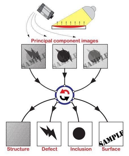
:Thermography is a powerful tool for non-destructive testing of a wide range of materials. Thermography has a number of approaches differing in both experiment setup and the way the collected data are processed. Among such approaches is the Principal Component Thermography (PCT) method, which is based on the statistical processing of raw thermal images collected by thermal camera. The processed images (principal components or empirical orthogonal functions) form an orthonormal basis, and often look like a superposition of all possible structural features found in the object under inspection—i.e., surface heating non-uniformity, internal defects and material structure. At the same time, from practical point of view it is desirable to have images representing independent structural features. The work presented in this paper proposes an approach for separation of independent image patterns (archetypes) from a set of principal component images. The approach is demonstrated in the application of inspection of composite materials as well as the non-invasive analysis of works of art.
1. Introduction
Thermography is a well-established approach in the non-destructive analysis of materials. It is based on the study of temperature distribution (and evolution of such a distribution with time) on the surface of the sample of interest. In most cases, the term “thermography” refers to the so-called “active” thermographic approach. Active thermography assumes the study of those temperature distributions which are induced by application of an external thermal impact—in contrast to “passive” thermography which generally deals with objects which are heated by natural sources or by other heat sources which are not set up intentionally for experiment (e.g., sunlight or natural body heat) [1,2,3,4]. This often makes the active thermography the only possible thermographic approach for the study of objects with no internal heat sources (e.g., composite and plastic panels for automotive applications).
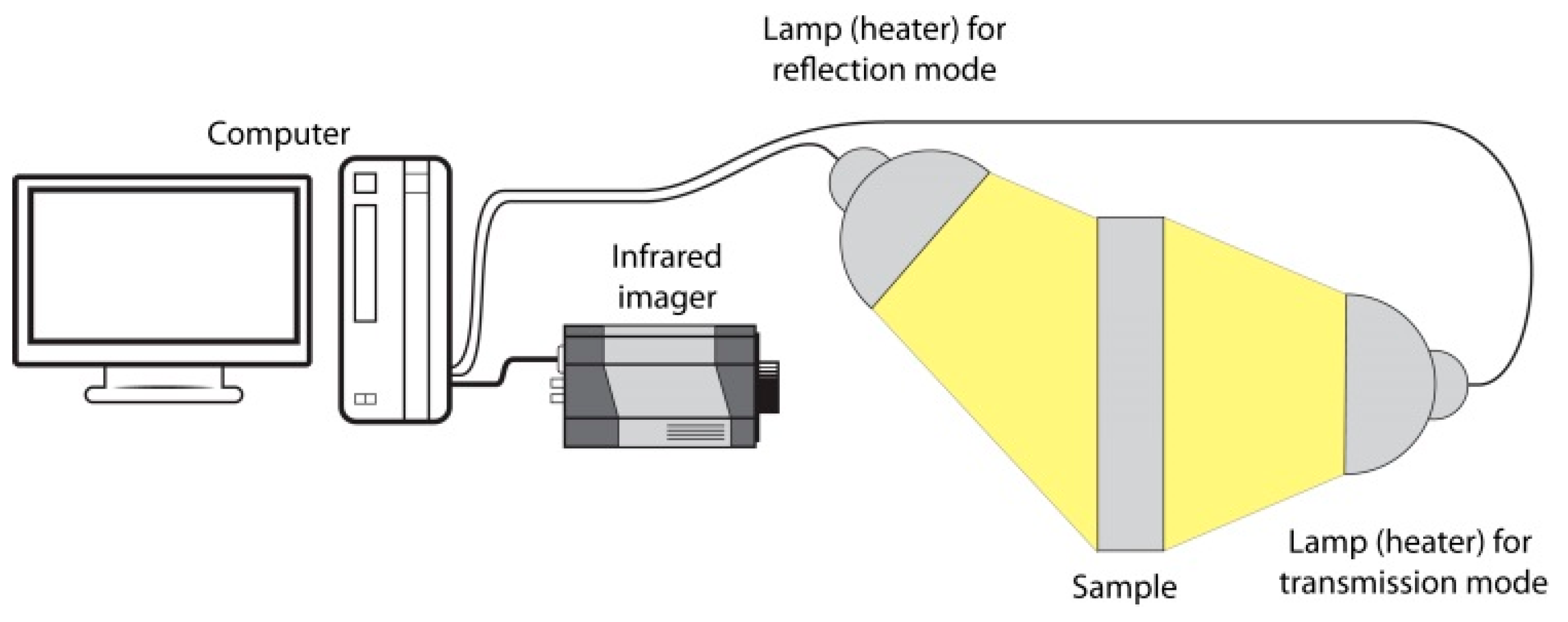
Active thermographic inspection (hereinafter thermography) requires two basic components: (a) thermal sensor and (b) the source of thermal impact (Figure 1). Although almost any thermal sensing device is applicable for use in thermographic experiments, modern thermography is generally performed with the use of thermal imagers (cameras). Thermal cameras allow one to obtain two-dimensional images showing the spatial distribution of temperature at the visible surface of the sample under analysis. Modern thermal cameras allow for the fast acquisition of such images, which creates possibilities for a large spectrum of potential experiments involving studies of how temperature distributions change with time (e.g., approaches of lock-in thermography, pulse phase thermography, etc.).
The second component of a thermographic setup is the source of thermal influence. The primary function of this component is to bring the object of interest out of thermal equilibrium and initiate heat flows—and temperature re-distribution—in the sample. While the temperature is forced to change, the thermal sensor collects information on this variation, and necessary conclusions are made from this information either with or without additional processing. From the practical point of view, the source of thermal influence is usually the source of heat, among which the most widely used sources are heat guns, lasers, and powerful xenon flash lamps. The choice of the source is highly dependent on the nature of the sample to be studied (e.g., for metals it could be an induction heat source while for plastic parts induction heat is inapplicable).
In the past few decades, thermography has found applications in numerous scientific fields and industries, paving the way from an exotic remote sensing method of warm objects to a quantitative method of non-destructive evaluation [5,6]. Modern thermographic techniques utilize fast and high-precision devices for collection of data about surface thermal distribution. At the same time, advanced computational processing of collected data is utilized in many modern thermographic approaches for extraction of quantitative information on structure and integrity of studied objects. Among such techniques are well-known approaches of lock-in thermography (LT) [7,8,9,10,11,12], pulse phase thermography (PPT) [11,13,14], thermal signal reconstruction (TSR) [11,15,16], and others. Most of these methods utilize various post-processing techniques in order to extract information regarding the structure and properties from the raw data on surface temperature distribution.
This work is related to one particular approach in active thermography, in particular, the Principal Component Thermography (PCT) and a proposed method for enhancing the results collected with this technique. Unlike conventional PCT method, the proposed approach allows for obtaining images which represent individual structural features of the sample under analysis (e.g., defects, internal structure). Images extracted with the proposed algorithm are more straightforward and suitable for interpretation than Principal Component images.
2. Methodology
Principal Component Thermography Approach
The Principal Component Thermography (PCT) technique was proposed by Rajic in 2002 [17] and has found application in the inspection of a wide variety of materials and components from industrial materials to the analysis of works of art. The theory and appropriate application procedures are well established and discussed in the literature (e.g., [18,19,20,21,22,23]).
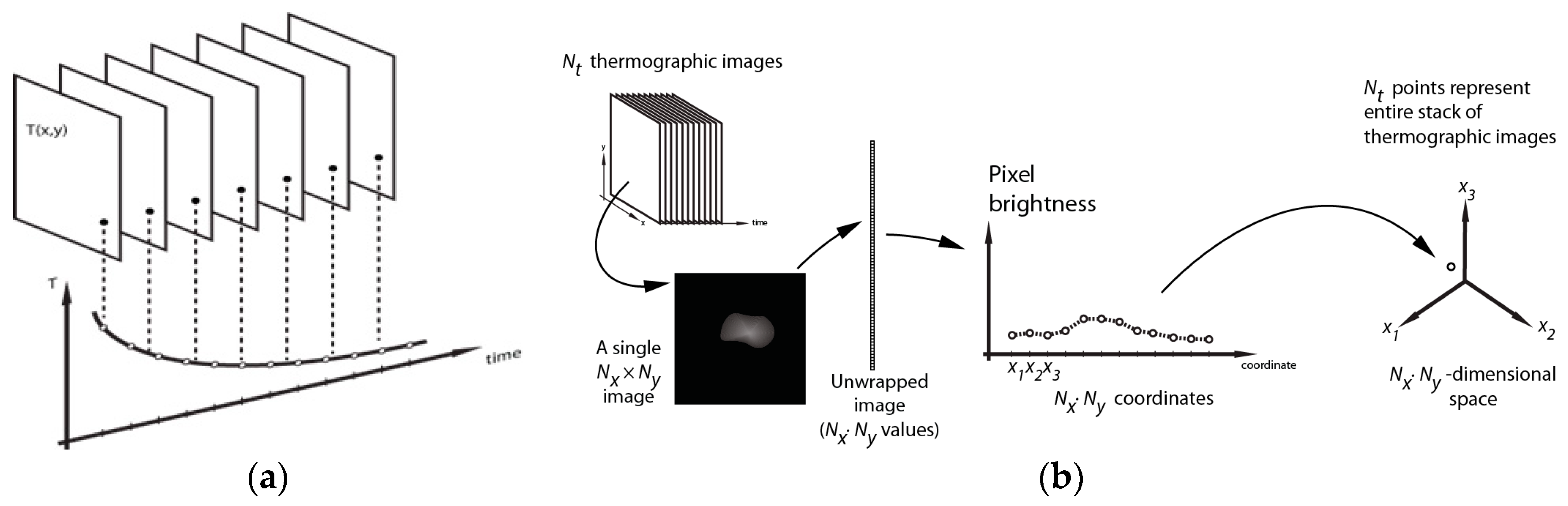
Unlike most other thermographic techniques, PCT is not based on a physical model, but rather utilizes a statistical approach to processing of raw data. In general terms, the procedure works as follows. The sample is brought out of thermal equilibrium, the thermal imager collects a series of thermal snapshots (Figure 2a), each of which is represented by a matrix of pixels (e.g., ). Each of these images can be treated as an array of values denoting brightnesses of each pixel (e.g., a image would contain 81,920 such values). If these values are treated as coordinates in a fictitious -dimensional space, each image can be treated as a single point in this space, where each of the coordinates is determined by brightness value of each of the pixels (Figure 2b). In such approach, images collected in an experiment can be treated as a cloud of points in -dimensional space (e.g., if someone collects 500 thermographic images with dimensions of , then such a sequence can be treated as 500 points in a fictitious 81,920-dimensional space formed by the brightness of each image pixel).
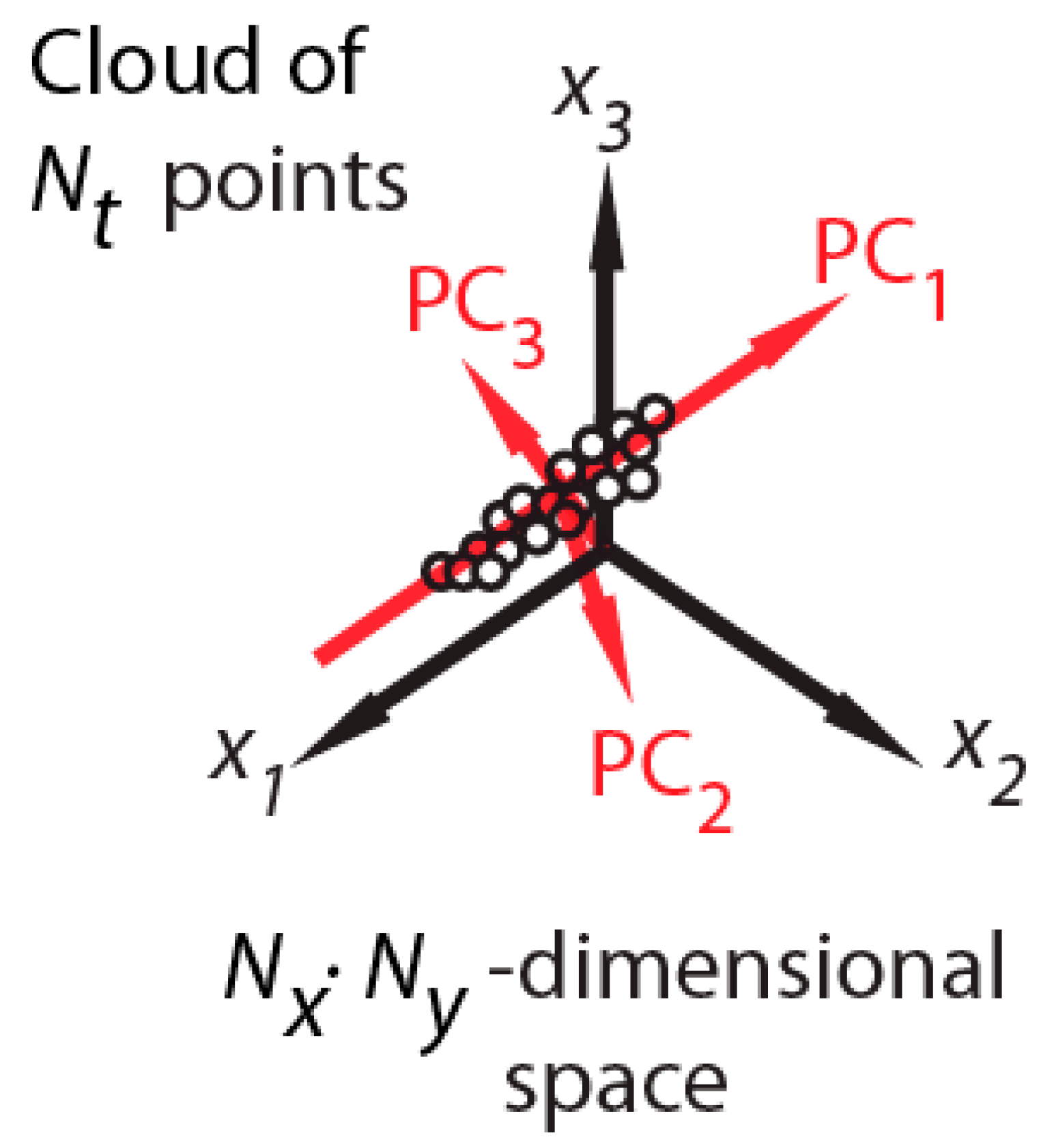
The “cloud” of such points is suitable for extraction of the so-called principal components (PCs). PCs represent a set of basis vectors constructed in such a way that the first principal component (PC1) describes most of the variance of the initial “cloud”, while each subsequent component describes most of the variance in the direction orthogonal to previous PCs (Figure 3). In many practical cases, a few first PCs determine the most variance of the initial data, and all remaining PCs determine only very small variations such as uncorrelated noises. This also allows for lossy compression of data by only preserving a few first principal components.
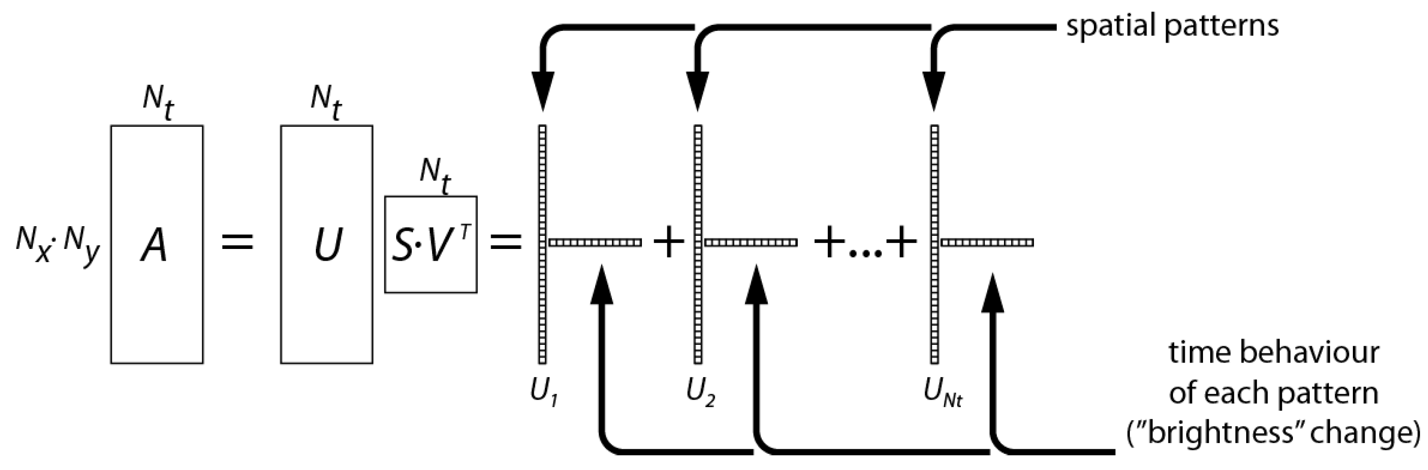
Extraction of the PCs can be performed with the aid of a well-known procedure known as Singular Value Decomposition (SVD):
In Expression (1), A represents a 2D matrix with its columns being thermal snapshots collected by imager unwrapped into 1D arrays. Matrix is the matrix of principal components, and its columns form an orthonormal basis. The rows of the matrix can be treated as the time evolution profile for each of the patterns (Figure 4).
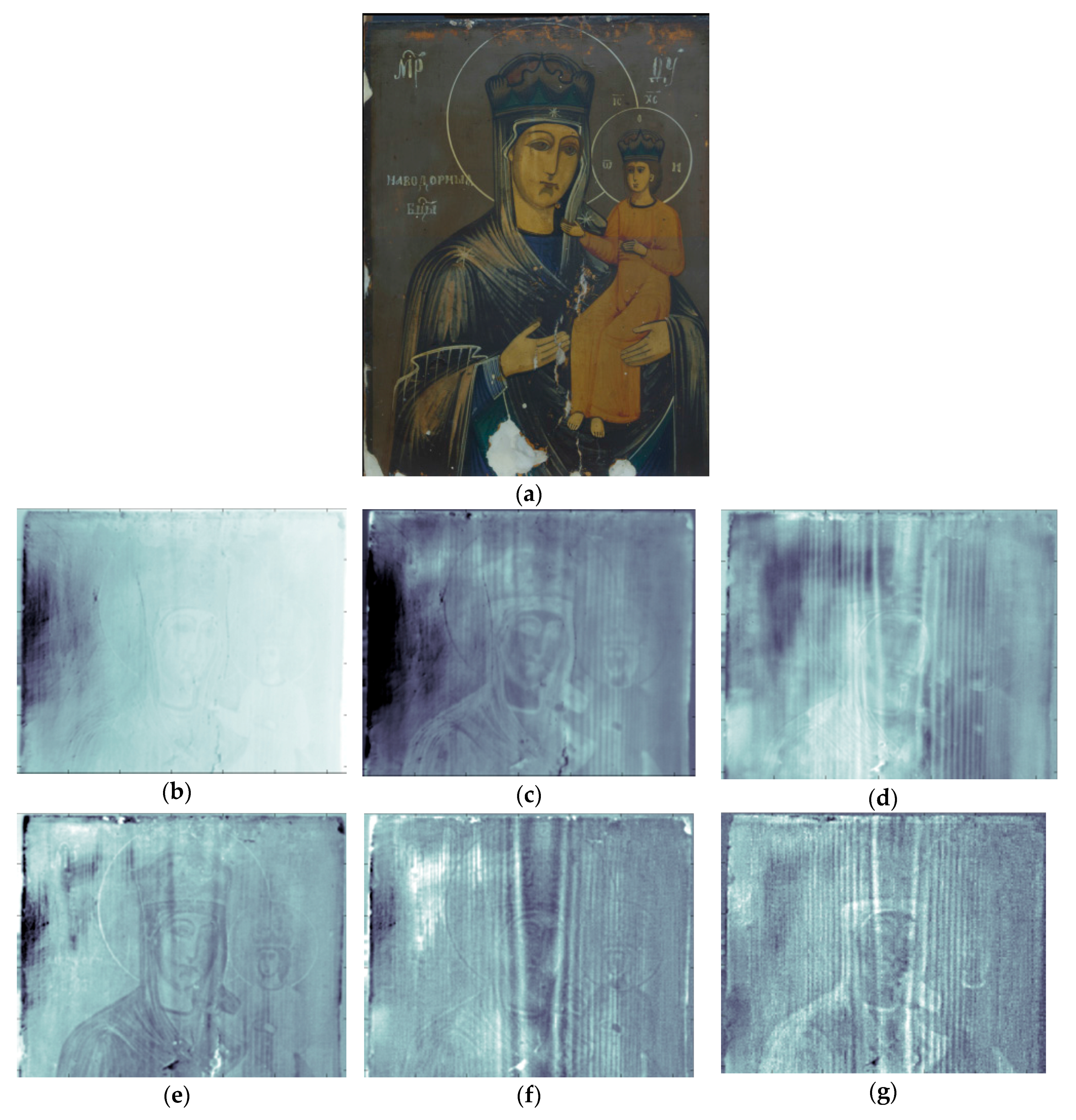
Let us have a look at a simple example of PCT. Figure 5 contains a few principal component images collected in a flash heat experiment on a piece of art. The sample represents an unattributed tempera/wood icon, 28 cm by 20.5 cm. The icon depicts a common “Madonna with the Child” scene. A few degradations are visible on the surface of the icon, and delamination defects are assumed to be possible.
Upon observation, the PC images higher than the 7th one demonstrate no visible image except for noise-like patterns. Higher PCs contain mostly white noise images (these images are not shown). The PCs shown in Figure 5 can be explained once again in the following way: each and every raw image collected by thermal imager (columns of matrix ) are linear combinations of the 7 principal images (and other numerous “noise” images which can be disregarded).
One important observation from Figure 5 is that the images do not explicitly show defects and the internal structure of the sample. Instead, the principal images are rather a superposition of various patterns. A set of PC images allows an experienced researcher to distinguish the patterns caused by surface heating non-uniformity, surface drawing (which is heated to different extents due to differences in colour), internal structure of the icon (wood grain pattern) as well as possible defect(s) in the top left corner.
3. Extraction of Independent Components
3.1. Proposed Approach
From a practical point of view, it would be desirable to have a set of images which would represent individual structural features such as surface drawing, structure and defects. On the other hand, the principal component images extracted by (1) have an important limitation—namely, they must form an orthonormal basis. In a general case, two independent images—e.g., images of overlapping defects—are not orthogonal, and thus such patterns cannot be acquired by the extraction of principal components.
At the same time, since PCs form an orthonormal basis, they can be used for construction of other images—including those which might not be orthogonal. This allows the possibility to use the extracted PCs for the construction of a set of (generally) non-orthogonal image patterns associated with the features of interest. The task is to find such a procedure which would allow for the construction of such independent patterns.
The procedure proposed here allows for construction of independent image patterns (hereinafter, archetypes) constructed of the principal component images. The following assumptions are made in this approach:
- Archetypes do exist.
- Existing archetype images do not necessarily form an orthonormal basis.
- Since principal components form a complete orthonormal basis, one can use this basis for constructing the archetypes.
- High-order principal components represent noise-like images and provide little information in the original stack of thermographic images. Thus, meaningful archetypes can be constructed using only a few low-order PCs.
- More than one PC may contain image patterns which belong to same archetype (e.g., the wood structure may be seen in PC2-7 in Figure 5). Thus, extraction of a single archetype requires using available PCs in such a way that an individual independent feature is extracted while all (or most) others are suppressed.
Let us assume that a stack of thermal images with sizes pixels has been acquired in an experiment, and each image was converted to 1D array of length in such a way that the data collected are represented by a 2D array . Assume that there is a set of 1D image arrays , where represents an empty image with i-th pixel set to unit brightness. Thus, each pattern can be expressed as
where can be treated as components of the vector , or, in other words, as brightness of j-th pixel of t-th image.
At the same time, set of archetypes can be used to represent any thermal pattern as:
where is the number of the archetype patterns present, and is the part of which cannot be determined by archetype patterns (e.g., image noise patterns). One can think of as an image, which means it can be represented as. Thus, from (2) and (3):
For fixed pixel with index m:
If we assume that pixel m only contains one archetype (), then
where determine the archetype image, and determines overall brightness modulation of that archetype. Thus, in Expression (6) brightness of one particular pixel is connected to brightnesses of the only archetype present in that point ().
Expression (6) allows for proposing the following principle for archetype image extraction. If an image stack is sorted in such a way that m-th pixel changes its brightness () according to a certain function (e.g., harmonically), then the brightness of an entire archetype owning that pixel () will change according to the same function. Thus, the following procedure can be proposed (schematically presented in Figure 6):
- Collect a stack of raw thermographic images and convert this stack to a 2D array
- Apply SVD to extract principal components.
- Leave only meaningful PCs (those which determine most of variance of raw data).
- Choose point(s) where only one independent pattern is present (e.g., only the pattern describing the defective area). These points are selected manually as it is important to find the point where only one independent pattern is present and thus Expression (6) is satisfied.
- Create a large number of random linear combinations from the PCs extracted. For research presented in this article, a set of 18,000 random combinations was constructed.
- Sort the new stack of images in such a way that the brightness of pixels in point(s) chosen change in a harmonic way.
- Find all pixels which happen to have similar modulation. These pixels belong to the same archetype which is present in the point(s) chosen.
3.2. Synthetic Example
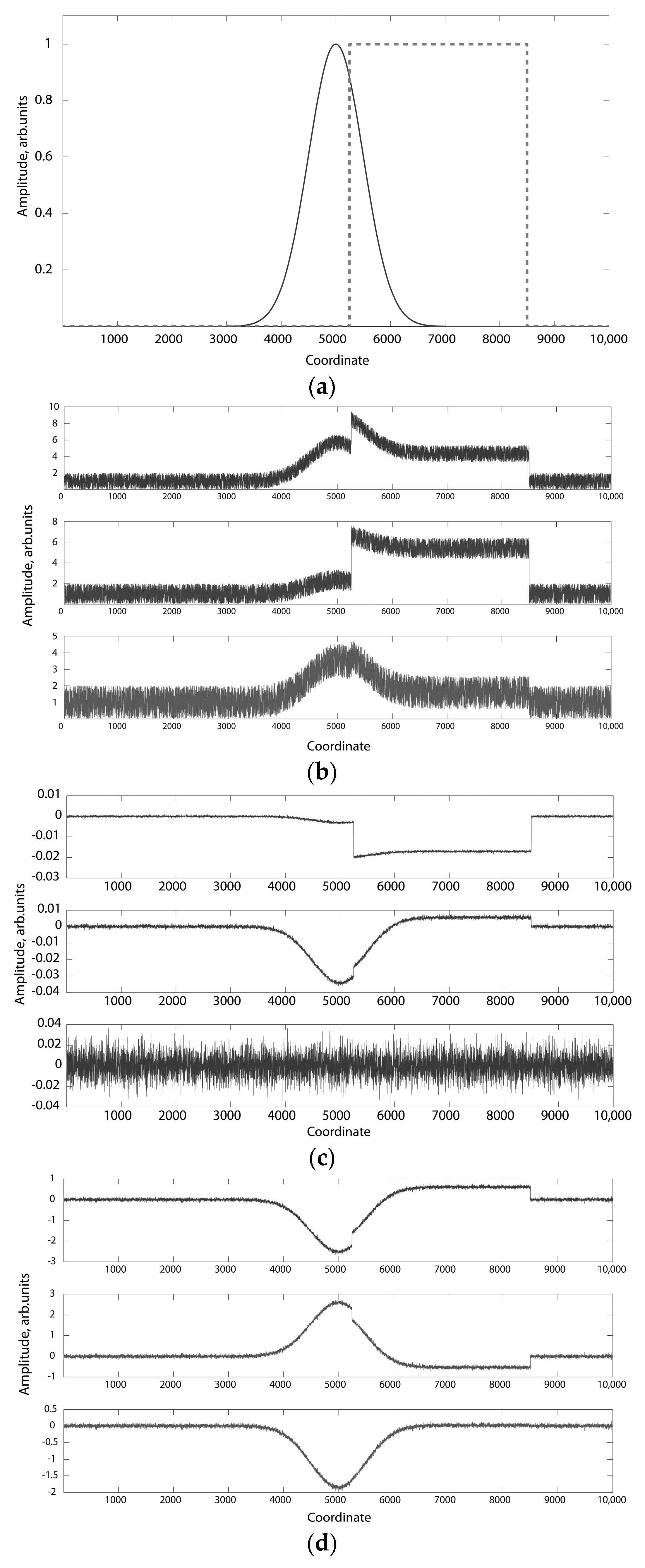
The proposed algorithm can be visualized in following way. Suppose that one has a set of random superpositions of two archetype patterns shown in Figure 7a. Examples of such combinations are shown in Figure 7b. The task is to extract archetype patterns from these random combinations. As can be seen from Figure 7c, the principal components cannot provide clear archetype patterns; both PC1 and PC2 are seen to be superpositions of the patterns to be found.
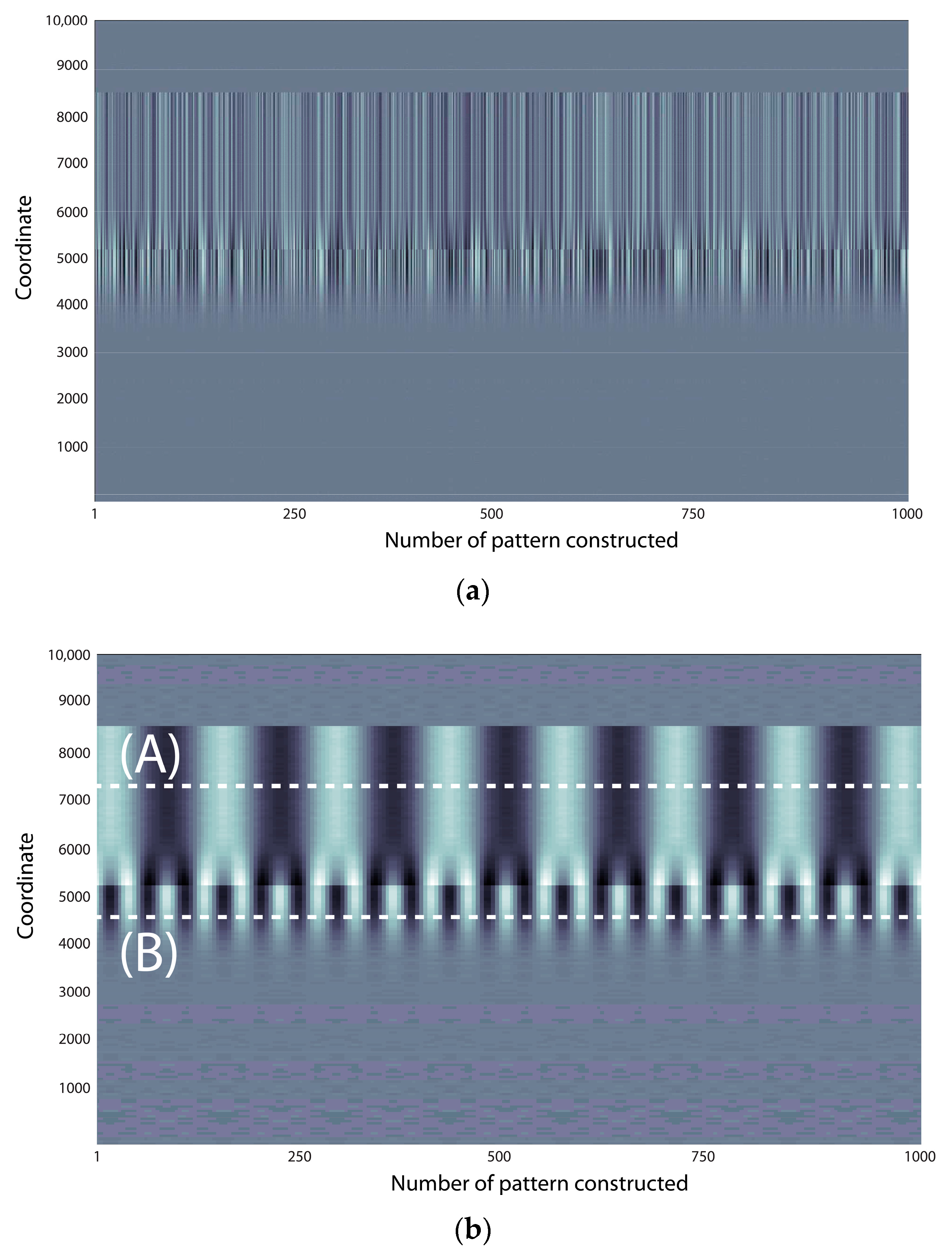
According to the procedure proposed above, one constructs a large number of linear combinations of PC1 and PC2 (examples of such patterns are given in Figure 7d). After constructing these linear combinations (in Figure 8a they are represented by columns of the image), two pixels are chosen for sorting the patterns. Each chosen point is assumed to belong to only one independent pattern to make Expression (6) work. As mentioned above, these points are to be chosen manually. This requires inspection of a few principal component images and making a decision on possible points.
4. Experimental Application of the Proposed Approach
4.1. Experimental Setup and Calculation Deta
All experiments discussed below were conducted using pulse heating and a reflection scheme of the thermographic setup. The thermal imager utilized was FLIR SC4000 (FLIR Systems, Wilsonville, OR, USA) with an InSb 320 × 256 focal plane array detector, sensitive in a 3–5 μm waveband set to 80 frames per second. Heating of the samples was done by a Speedotron 4803CX system (Speedotron Corporation, Bartlett, IL, USA) equipped with a single Speedotron 206VF light unit (MW40QC xenon lightbulb, UV coated) (Speedotron Corporation, Bartlett, IL, USA)
At the stage of construction of random combinations of Principal Component images, a set of 18,000 combinations was created. The resulting set of data (assuming single data precision) was nearly 1.5 Gb and was processed on a PC with 24 Gb RAM, 3.8 GHz CPU with dedicated GPU video (which allowed for fast parallel processing). Weighting factors were randomly chosen between 0 and 1.
4.2. Non-Destructive Analysis of Works of Art
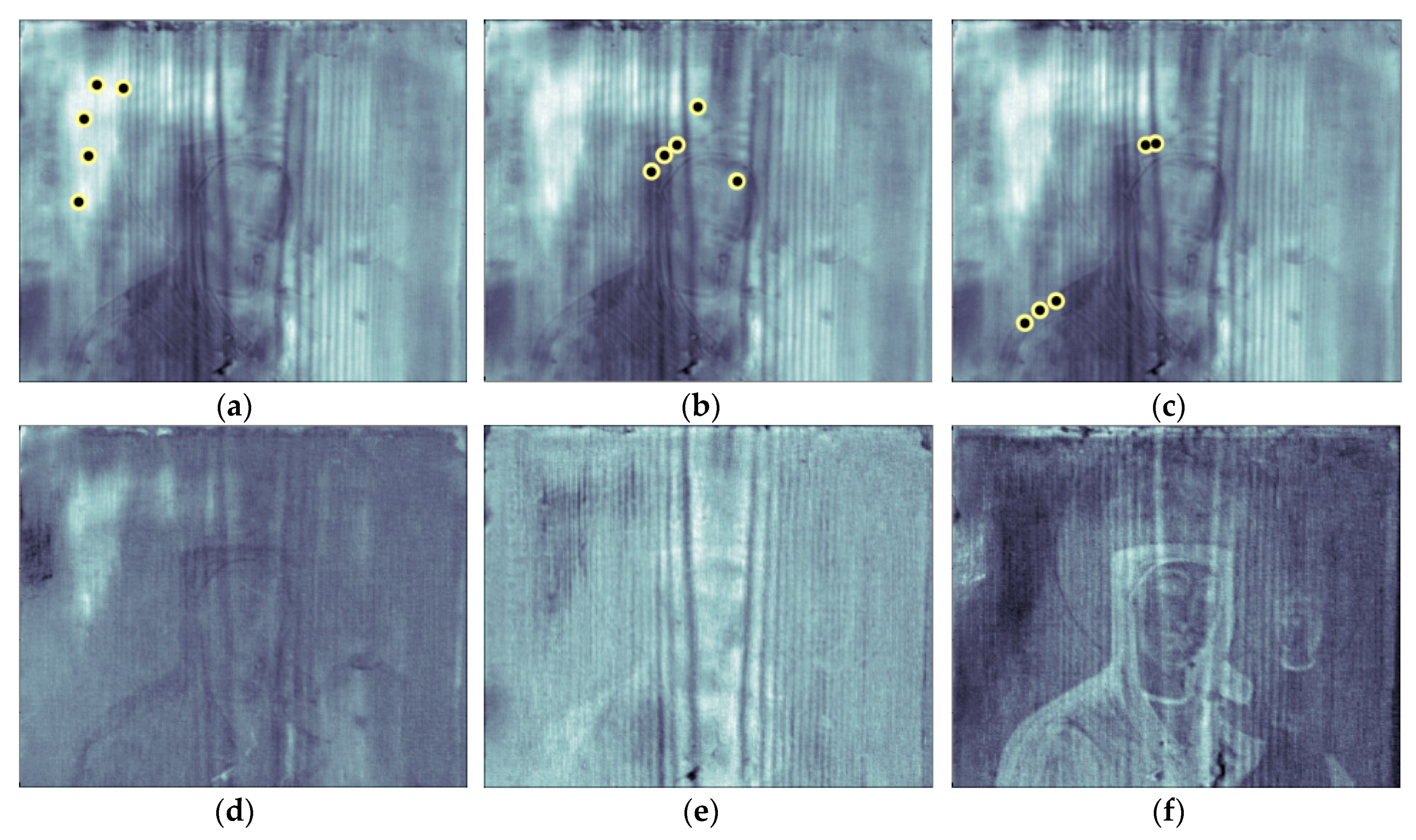
The first example will be given using the same tempera icon mentioned above. As can be seen from Figure 5, only 7 PCs demonstrate recognizable patterns which can be associated with features of interest. These PCs were used for construction of 18,000 random combinations, and then sorted in an appropriate way. After that, procedure independent patterns were extracted, as presented in Figure 10.
As can be seen, the patterns extracted have much fewer common features than the initial PCs used for their construction, and every pattern mostly displays a logically independent feature—e.g., the wood grains, the defect or the surface drawing. The patterns are not totally free from common features (e.g., the surface drawing may be recognized in the pattern corresponding to the “defect”), although this gives a good illustration of the general procedure for extracting archetype images.
4.3. Inspection of Composite Materials
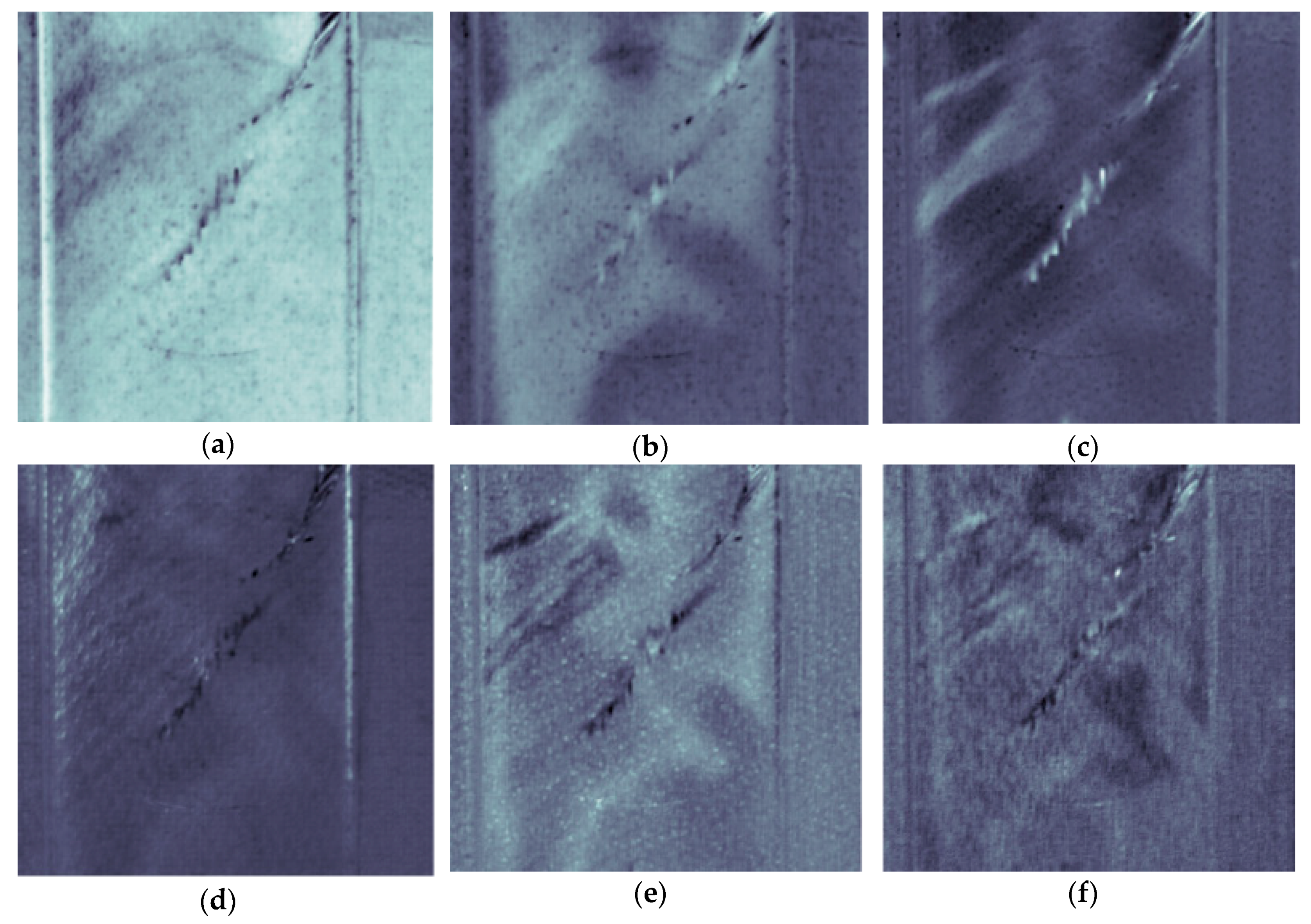
The composite material tested was a 140 mm × 140 mm piece of Bombardier C-series wing skin. The piece was intentionally damaged by a quasi-static loading procedure, during which the sample was pressed by a 20 mm hemi-spherical indenter with a force of 46,615 N (maximum indentation was about 16.5 mm, and the sample was visibly damaged) [25]. After the loading test, the sample was used for collecting raw thermographic images in a standard way with a xenon flash heat stimulation. The PCs collected are shown in Figure 11.
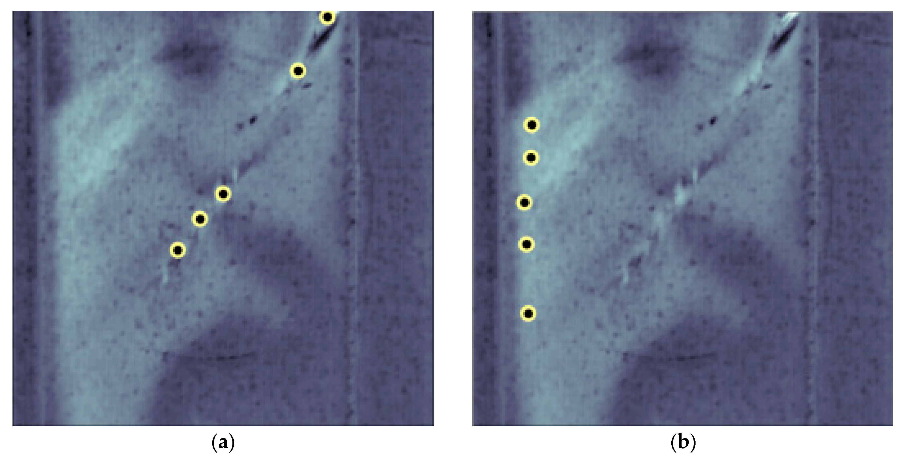
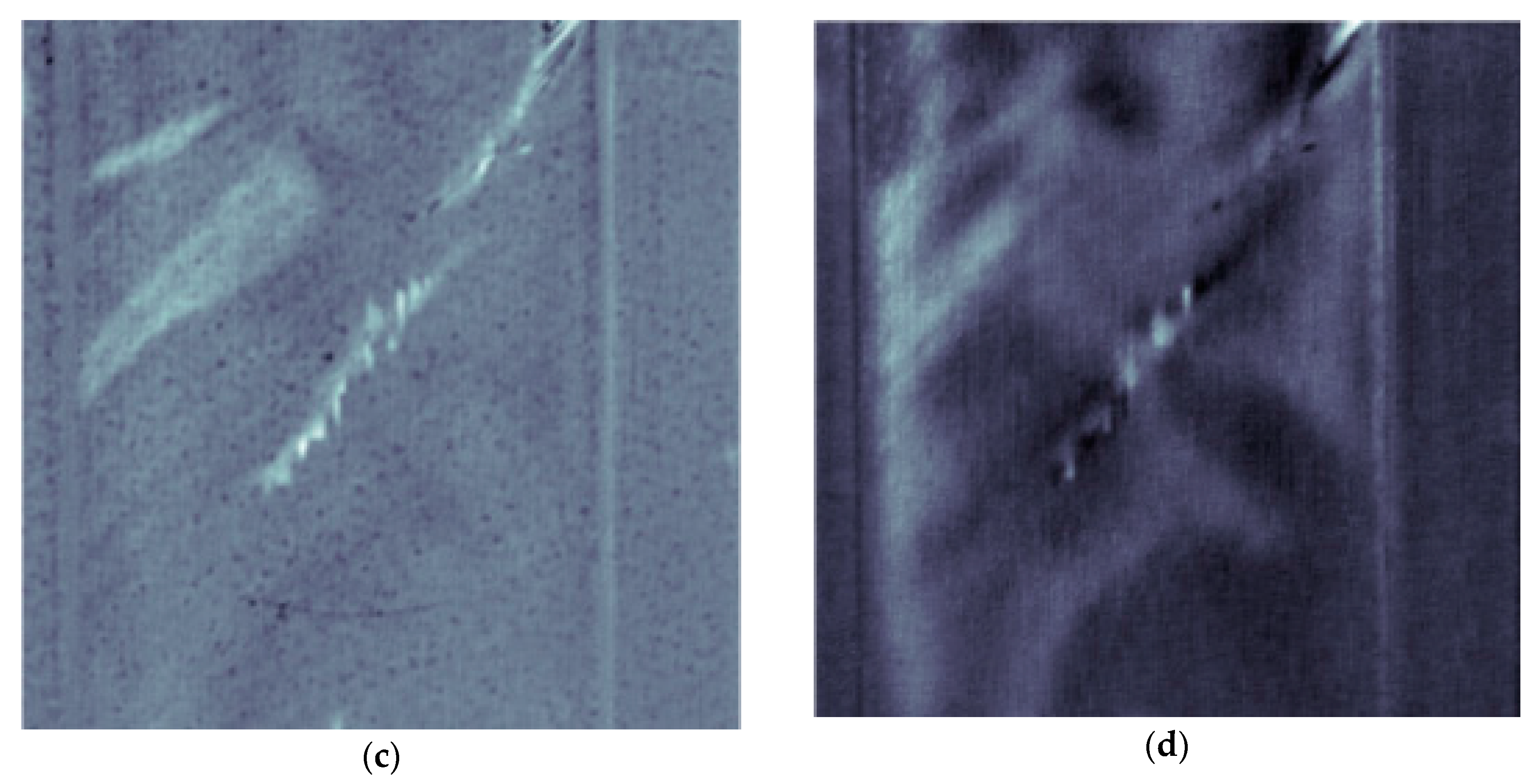
As can be seen from Figure 11, two separate major defects are present. An attempt to collect separate independent images of these defects led to the results demonstrated in Figure 12. It appears that one of the defects is a serious delamination covering almost the entire area of the sample, while the other is a smaller detachment.
5. Conclusions
Traditional Principal Component images extracted from raw thermographic data provide clear images which can be used for visualization of structural features such as defects, inclusions, surface heating non-uniformities and so on. This becomes possible because most variance of an entire data set becomes concentrated in a few low order principal components, while high-order components only contain uncorrelated noisy patterns. Extraction of these images forms the core of Principal Component thermography (PCT). Among the drawbacks of PCT images is its inability to provide independent images of individual structural features of the sample under inspection. In particular, the requirement of orthogonality of extracted images (columns of matrix in Expression (1)) leads to the fact that a number of principal images may share contours of the same features (e.g., intersecting defects).
The approach proposed in this work allows for use of the principal images extracted by a conventional PCT approach as a basis for constructing a new set of images corresponding to independent structural patterns. Construction of such patterns requires appropriate sorting of a set of random combinations of meaningful PC images and finding those pixels which would exhibit similar sorting type. In this work, the approach has been demonstrated as capable of extracting nearly unmixed patterns of defects, internal structure and surface heating. It may be that the approach proposed could be valuable when it is necessary to extract unbiased images of particular structural features, i.e., with minimal inclusion of noise and patterns associated with other structural features.
For effective work of the algorithm, manual selection of a few points where no independent images overlap is required. Automatic selection of such points would be the next development step.
Acknowledgments
The authors express their gratitude to Bombardier Aerospace for the samples of C-series composite structures provided.
Author Contributions
The presented work was completed under the supervision of Roman Gr. Maev, based on the work of Dmitry Gavrilov.
Conflicts of Interest
The authors declare no conflict of interest.
References
- Janků, M.; Březina, I.; Grošek, J. Use of Infrared Thermography to Detect Defects on Concrete Bridges. Procedia Eng. 2017, 190, 62–69. [Google Scholar] [CrossRef]
- Lagüela, S.; Solla, M.; Armesto, J.; González-Jorge, H. Comparison of infrared thermography with ground-penetrating radar for the non-destructive evaluation of historic masonry bridges. In Proceedings of the 11th International Conference on Quantitative InfraRed Thermography (QIRT 2012), Naples, Italy, 11–14 June 2012. [Google Scholar]
- Soroko, M.; Howell, K. Infrared Thermography: Current Applications in Equine Medicine. J. Equine Vet. Sci. 2018, 60, 90–96. [Google Scholar] [CrossRef]
- Kandlikar, S.G.; Perez-Raya, I.; Raghupathi, P.A.; Gonzalez-Hernandez, J.-L.; Dabydeen, D.; Medeiros, L.; Phatak, P. Infrared imaging technology for breast cancer detection—Current status, protocols and new directions. Int. J. Heat Mass Transf. 2017, 108, 2303–2320. [Google Scholar] [CrossRef]
- Vavilov, V. Thermal Non-Destructive Testing: Short History, State-of-the-Art and Trends. In Proceedings of the 10th European Conference on Non-Destructive Testing (ECNDT), Moscow, Russia, 7–11 June 2010. [Google Scholar]
- Vavilov, V. Thermal non destructive testing: Short history and state-of-art. In Proceedings of the 1992 International Conference on Quantitative InfraRed Thermography (QIRT), Paris, France, 7–9 July 1992. [Google Scholar]
- Delanthabettu, S.; Menaka, M.; Venkatraman, B.; Raj, B. Defect depth quantification using lock-in thermography. QIRT J. 2015, 12, 37–52. [Google Scholar] [CrossRef]
- Fedala, Y.; Streza, M.; Sepulveda, F.; Roger, J.-P.; Tessier, G.; Boué, C. Infrared lock-in thermography crack localization on metallic surfaces for industrial diagnosis. JNDE 2014, 33, 335–341. [Google Scholar] [CrossRef]
- Breitenstein, O.; Warta, W.; Langenkamp, M. Lock-in Thermography: Basics and Use for Evaluating Electronic Devices and Materials, 2nd ed.; Springer: Berlin/Heidelberg, Germany, 2010; pp. 22–26. ISBN 978-3-642-02416-0. [Google Scholar]
- Nolte, P.; Malvisalo, T.; Wagner, F.; Schweiser, S. Thermal diffusivity of metals determined by lock-in thermography. QIRT J. 2017, 14, 218–225. [Google Scholar] [CrossRef]
- D’Accardi, E.; Palumbo, D.; Tamborrino, R.; Galietti, U. Quantitative analysis of thermographic data through different algorithms. Proc. Struct. Integr. 2018, 8, 354–367. [Google Scholar] [CrossRef]
- Ciampa, F.; Mahmoodi, P.; Pinto, F.; Meo, M. Recent Advances in Active Infrared Thermography for Non-Destructive Testing of Aerospace Components. Sensors 2018, 18, 609. [Google Scholar] [CrossRef] [PubMed]
- Maldague, X.; Marinetti, S. Pulse Phase Infrared Thermography. J. Appl. Phys. 1996, 79, 2694–2698. [Google Scholar] [CrossRef]
- Ibarra-Castanedo, C.; Sfarra, S.; Ambrosini, D.; Paoletti, D.; Bendada, A.; Maldague, X. Subsurface defect characterization in artworks by quantitative pulsed phase thermography and holographic interferometry. QIRT J. 2008, 5, 131–149. [Google Scholar] [CrossRef]
- Shepard, S.M.; Hou, Y.; Ahmed, T.; Lhota, J.R. Reference-free analysis of flash thermography data. Proc. SPIE 2006, 6205, 1–7. [Google Scholar] [CrossRef]
- Shepard, S.M. Advances in Pulsed thermography. Proc. SPIE 2001, 4360, 511–515. [Google Scholar]
- Rajic, N. Principal component thermography for flaw contrast enhancement and flaw depth characterization in composite structures. Compos. Struct. 2002, 58, 521–528. [Google Scholar] [CrossRef]
- Marinetti, S.; Grinzato, E.; Bison, P.G.; Bozzi, E.; Chimenti, M.; Pieri, G.; Salvetti, O. Statistical analysis of IR thermographic sequences by PCA. Infrared Phys. Technol. 2004, 46, 85–91. [Google Scholar] [CrossRef]
- Vavilov, V.P.; Nesteruk, D.A.; Shiryaev, V.V.; Swiderski, W. Application of principal component analysis in dynamic thermal testing data processing. Russ. J. Nondestruct. 2008, 44, 509–516. [Google Scholar] [CrossRef]
- Griefahn, D.; Wollnack, J.; Hintze, W. Principal component analysis for fast and automated thermographic inspection of internal structures in sandwich parts. J. Sens. Sens. Syst. 2014, 3, 105–111. [Google Scholar] [CrossRef]
- Świta, R.; Suszyński, Z. Processing of thermographic sequence using principal component analysis. Meas. Autom. Monitor. 2015, 61, 215–218. [Google Scholar]
- Gavrilov, D.; Maev, R.G.; Almond, D. A review of imaging methods in analysis of works of art. Thermographic imaging method in art analysis. Can. J. Phys. 2014, 92, 341–364. [Google Scholar] [CrossRef]
- Yousefi, B.; Sfarra, S.; Ibarra-Castanedo, C.; Maldague, X. Comparative analysis on thermal non-destructive testing imagery applying Candid Covariance-Free Incremental Principal Component Thermography (CCIPCT). Infrared Phys. Technol. 2017, 85, 163–169. [Google Scholar] [CrossRef]
- Gavrilov, D. Development and Optimization of Thermographic Techniques for Non-Destructive Evaluation of Multilayered Structures. Ph.D. Thesis, University of Windsor, Windsor, ON, Canada, 2014. [Google Scholar]
- Bondy, M.; Gavrilov, D.; Seviaryna, I.; Maev, R. Practical application of acoustic and thermographic methods for analysis of impact damage to composite avionic parts. In Proceedings of the 14th International Workshop on Advanced Infrared Technology and Applications (AITA 2017), Quebec City, QC, Canada, 27–29 September 2017. [Google Scholar]
Figure 1.
Basic thermographic setup scheme.

Figure 2.
(a) Explanation of stack of thermal images; (b) Illustration of multidimensional representation of each thermal image in stack (only first three of all dimensions are shown).
Figure 2.
(a) Explanation of stack of thermal images; (b) Illustration of multidimensional representation of each thermal image in stack (only first three of all dimensions are shown).

Figure 3.
Explanation of Principal Components (only three dimensions are shown). Red arrows indicate the directions of the first three principal components [24].
Figure 3.
Explanation of Principal Components (only three dimensions are shown). Red arrows indicate the directions of the first three principal components [24].

Figure 4.
Explanation of Singular Value Decomposition (SVD) [24].
Figure 4.
Explanation of Singular Value Decomposition (SVD) [24].

Figure 5.
Examples of principal components (PCs) extracted: (a) General view of the inspected object; (b) PC1; (c) PC2; (d) PC3; (e) PC4; (f) PC5; (g) PC6; (h) PC7; (i) PC8; (j) PC9.
Figure 5.
Examples of principal components (PCs) extracted: (a) General view of the inspected object; (b) PC1; (c) PC2; (d) PC3; (e) PC4; (f) PC5; (g) PC6; (h) PC7; (i) PC8; (j) PC9.


Figure 6.
Explanation of the algorithm. The red and blue graphs schematically indicate how brightnesses of two particular pixels change through the stack of the sorted images.
Figure 6.
Explanation of the algorithm. The red and blue graphs schematically indicate how brightnesses of two particular pixels change through the stack of the sorted images.
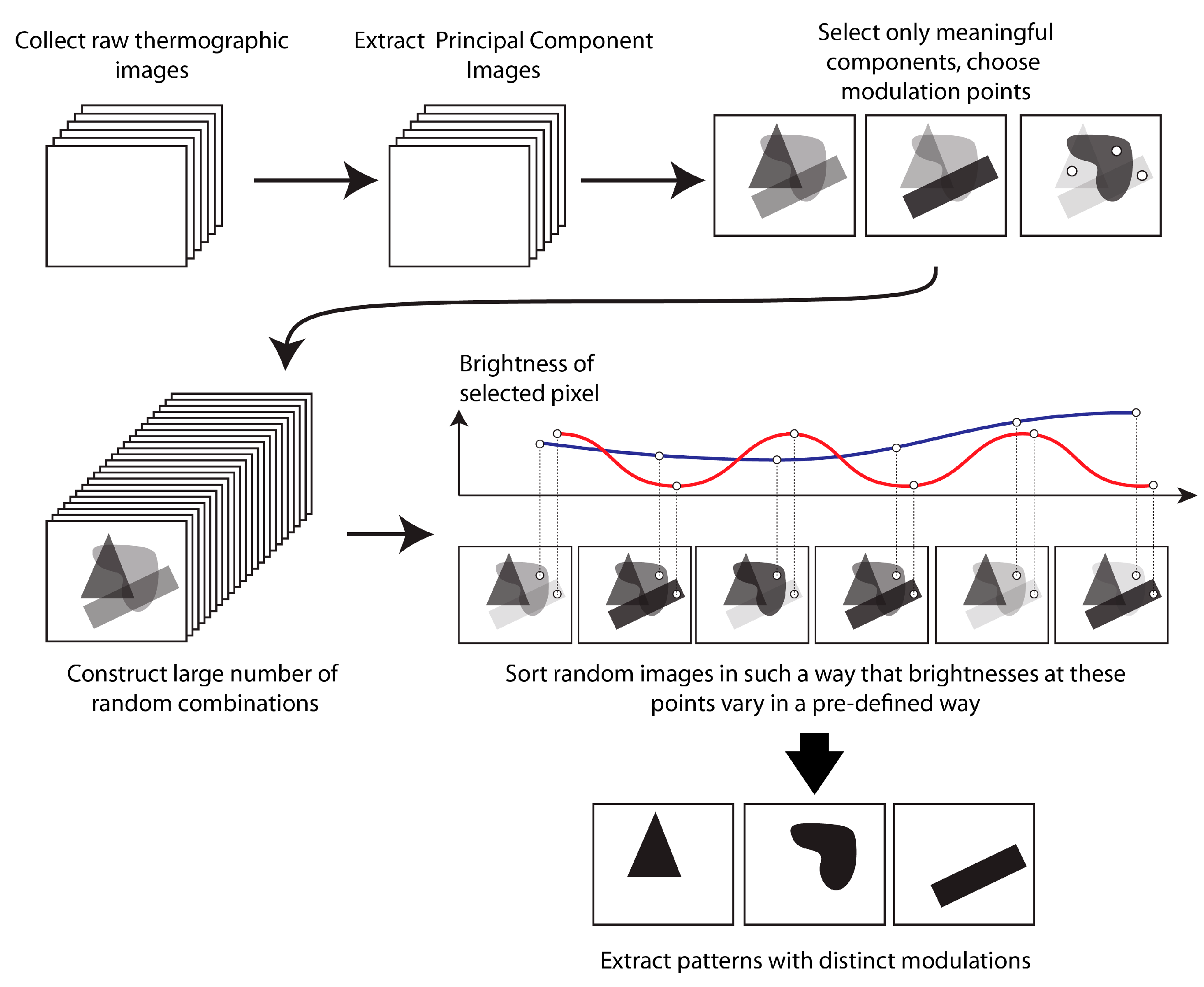
Figure 7.
Two 1D archetype functions example: (a) the general form of the archetypes; (b) examples of noisy superpositions of the archetypes (raw patterns); (c) the first three PCs for the set of raw patterns, (d) examples of random superpositions of PC1 and PC2.
Figure 7.
Two 1D archetype functions example: (a) the general form of the archetypes; (b) examples of noisy superpositions of the archetypes (raw patterns); (c) the first three PCs for the set of raw patterns, (d) examples of random superpositions of PC1 and PC2.

Figure 8.
A set of random patterns constructed from the first principal components: (a) unsorted patterns; (b) sorted patterns. The dashed lines indicate the positions of the two reference points (denoted as A and B).
Figure 8.
A set of random patterns constructed from the first principal components: (a) unsorted patterns; (b) sorted patterns. The dashed lines indicate the positions of the two reference points (denoted as A and B).

Figure 9.
Reconstruction of 1D archetype shapes: (a) amplitude spectrum; (b) reconstructed profiles (different colours are used to distinguish between two reconstructed archetypes).
Figure 9.
Reconstruction of 1D archetype shapes: (a) amplitude spectrum; (b) reconstructed profiles (different colours are used to distinguish between two reconstructed archetypes).

Figure 10.
Examples of reconstructed structural images (archetypes): (a) points chosen for “defect”; (b) points chosen for “structure”; (c) points chosen for “drawing”; (d) reconstructed “defect”; (e) reconstructed “structure”; (f) reconstructed “drawing”.
Figure 10.
Examples of reconstructed structural images (archetypes): (a) points chosen for “defect”; (b) points chosen for “structure”; (c) points chosen for “drawing”; (d) reconstructed “defect”; (e) reconstructed “structure”; (f) reconstructed “drawing”.

Figure 11.
PCs extracted from a set of thermographic images collected from a composite material piece (side opposite to loading): (a) PC1; (b) PC2; (c) PC3; (d) PC4; (e) PC5; (f) PC6.
Figure 11.
PCs extracted from a set of thermographic images collected from a composite material piece (side opposite to loading): (a) PC1; (b) PC2; (c) PC3; (d) PC4; (e) PC5; (f) PC6.

Figure 12.
Examples of reconstructed structural images (archetypes) for a damaged composite plate: (a) points chosen for “defect #1”; (b) points chosen for “defect #2”; (c) reconstructed “defect #1”; (d) reconstructed “defect #2”.
Figure 12.
Examples of reconstructed structural images (archetypes) for a damaged composite plate: (a) points chosen for “defect #1”; (b) points chosen for “defect #2”; (c) reconstructed “defect #1”; (d) reconstructed “defect #2”.


© 2018 by the authors. Licensee MDPI, Basel, Switzerland. This article is an open access article distributed under the terms and conditions of the Creative Commons Attribution (CC BY) license (http://creativecommons.org/licenses/by/4.0/).
Share and Cite
MDPI and ACS Style
Gavrilov, D.; Maev, R.G. Extraction of Independent Structural Images for Principal Component Thermography. Appl. Sci. 2018, 8, 459. https://doi.org/10.3390/app8030459
AMA Style
Gavrilov D, Maev RG. Extraction of Independent Structural Images for Principal Component Thermography. Applied Sciences. 2018; 8(3):459. https://doi.org/10.3390/app8030459
Chicago/Turabian StyleGavrilov, Dmitry, and Roman Gr. Maev. 2018. "Extraction of Independent Structural Images for Principal Component Thermography" Applied Sciences 8, no. 3: 459. https://doi.org/10.3390/app8030459
Note that from the first issue of 2016, this journal uses article numbers instead of page numbers. See further details here.