Deep Activation Pooling for Blind Image Quality Assessment


1
Tianjin Key Laboratory of Wireless Mobile Communications and Power Transmission, Tianjin Normal University, Tianjin 300387, China
2
College of Electronic and Communication Engineering, Tianjin Normal University, Tianjin 300387, China
3
Department of Electronic and Electrical Engineering, University of Strathclyde, Glasgow Scotland G1 1XQ , UK
*
Author to whom correspondence should be addressed.
Appl. Sci. 2018, 8(4), 478; https://doi.org/10.3390/app8040478
Submission received: 30 January 2018
/
Revised: 15 March 2018
/
Accepted: 19 March 2018
/
Published: 21 March 2018
Abstract
:Driven by the rapid development of digital imaging and network technologies, the opinion-unaware blind image quality assessment (BIQA) method has become an important yet very challenging task. In this paper, we design an effective novel scheme for opinion-unaware BIQA. We first utilize the convolutional maps to select high-contrast patches, and then we utilize these selected patches of pristine images to train a pristine multivariate Gaussian (PMVG) model. In the test stage, each high-contrast patch is fitted by a test MVG (TMVG) model, and the local quality score is obtained by comparing with the PMVG. Finally, we propose the deep activation pooling (DAP) to automatically emphasize the more important scores and suppress the less important ones so as to obtain the overall image quality score. We verify the proposed method on two widely used databases, that is, the computational and subjective image quality (CSIQ) and the laboratory for image and video engineering (LIVE) databases, and the experimental results demonstrate that the proposed method achieves better results than the state-of-the-art methods.
1. Introduction
Nowadays, there are many applications [1,2], such as image transmission, acquisition, compression, enhancement and analysis, that require an efficient and accurate algorithm for image quality assessment (IQA). Generally, the IQA methods can be separated into two major classes: subjective assessment and objective assessment. As the final evaluation criterion of an image, the subjective assessment is mainly conducted by the pretrained human observers, which is time-consuming and labour-intensive. Hence, more and more researchers are devoted to the development of objective IQA methods that can automatically evaluate the image quality. One trend is to develop full reference IQA (FR–IQA) algorithms when the pristine reference image is available. For example, Kim et al. [3] utilized the difference of gradients between the source and distorted images to evaluate the image quality. Zhang et al. [4] proposed a novel feature similarity (FSIM) index which combines the phase information with image gradient magnitudes for FR–IQA. Xue et al. [5] presented the gradient magnitude similarity deviation (GMSD) and achieved impressive accuracy. However, these FR–IQA methods evaluate image quality by using the pristine reference images, which are usually unavailable.
To overcome the above-mentioned limitation, many no-reference IQA (NR–IQA) methods [6,7,8,9] have been proposed. Early NR–IQA methods assume that the assessed images are influenced by one or multiple types of known distortions, for example, ringing, blockiness or compression, and meanwhile, the IQA models are designed for these known distortions. Hence, the application field of these approaches is very limited. The blind IQA (BIQA) is a new trend of NR–IQA research, and it does not need to know the distortion types. Most existing BIQA methods are opinion-aware [10,11,12,13], which trains a regression model from numerous training images (source and distortion images) with the homologous human subjective scores. Specifically, the features are first obtained from the training images, and then both feature vectors and corresponding human subjective scores are employed to train a regression model. In the test stage, the feature vector of an image is fed into the trained regression model to generate the quality score. In [12], Li et al. utilized several perceptually relevant image features for the opinion-aware BIQA task. The features contain the entropy and mean value of phase congruency image, and the entropy and gradient of the distorted image. Mittal et al. [14] proposed the blind/referenceless image spatial quality evaluator (BRISQUE) to assess image quality. In [15], Zhang and Chandler proposed an efficient NR–IQA algorithm using a log-derivative statistical model of natural scenes. Xue et al. [16] combined the normalized gradient magnitude (GM) with the Laplacian of Gaussian (LOG) features to learn a regression model. There are two main drawbacks of opinion-aware BIQA. Firstly, the approach requires a large amount of distorted images to learn the regression model. In practice, however, it is a challenging task to collect enough training images to cover all kinds of distortions. Secondly, since the image distortion types are diverse and there may be several interacting distortions contained in one image, the opinion-aware BIQA models have a weak generalization ability. This means that the image quality scores are often inaccurate when the model learned from one database is directly applied to another one.
Recently, many researchers have turned to the attractive and challenging study of the opinion-unaware BIQA methods, which only use the pristine naturalistic images to train a model. The opinion-unaware BIQA methods are independent of the distorted images and relevant subjective quality scores, and therefore they possess more potential to deliver higher generalization capability than the opinion-aware ones. In [17], the quality score is described as a simple distance metric between the distorted image and the model statistic. Xue et al. [18] proposed the quality-aware clustering scheme to assess the quality levels of image patches. Zhang et al. [19] proposed the integrated local natural image quality evaluator (IL–NIQE) to predict image quality for opinion-unaware BIQA tasks. Firstly, they utilize five types of features to obtain the feature vectors of pristine naturalistic images, that is, the mean-subtracted contrast normalized (MSCN)-based features, MSCN product-based features, gradient-based features, log-Gabor response-based features and color-based features. Secondly, they use the feature vectors of pristine images to train a MVG model. Then, each patch in the test image is utilized to train a MVG model, and the parameters of the MVG model are compared with the trained MVG model to generate a quality score for the local patch. Finally, the overall quality score is computed by using the average pooling strategy. However, the average pooling lacks discrimination because the contributions of the patches are equally treated, whatever their importances are.
In this paper, we propose a novel approach for opinion-unaware BIQA. Figure 1 illustrates the procedure of the proposed approach. Firstly, we utilize the convolutional maps of a pretrained convolutional neural network (CNN) for high-contrast patch selection. The convolutional activations represent the structural and textural features, and therefore the selection process could choose the salient patches and drop the meaningless ones for the subsequent assessment. Then, we utilize these selected patches of pristine images to train a pristine multivariate Gaussian (PMVG) model. In the test stage, each high-contrast patch in the test image is fitted by a test MVG (TMVG) model, and the local quality score is obtained by comparing with the PMVG. Finally, the deep activation pooling (DAP) is proposed to aggregate these local quality scores into an overall image quality score. We employ the convolutional summing map (CSM) computed from the convolutional layer to learn the aggregating weights. Specifically, each selected high-contrast patch is mapped to the corresponding activation-response region, and all the activation responses in the corresponding region are added as the aggregating weight. Hence, the proposed DAP could automatically obtain the aggregating weights by learning the importance of local quality scores from the CSM.
In summary, the major contributions of this paper are: (1) We use the high-contrast patches chosen based on convolutional activations to train the PMVG and TMVG models, which captures the primary structural and textural information of images and obtains more accurate PMVG and TMVG models; (2) we compute local quality scores based on the PMVG and TMVG models, and propose the DAP to automatically learn the aggregating weights of local quality scores from CSM, which produces more accurate overall quality score.
2. Approach
In this section, we first describe the convolutional summing map (CSM) of VGG-19 [20], which is utilized for selecting high-contrast patches and learning pooling weights. Afterwards, we present the high-contrast selection processing and the DAP strategy.
2.1. Convolutional Summing Map
In the convolutional layer of a CNN, the filters traverse the image in a sliding-window manner to generate convolutional maps. The convolutional maps can be regarded as a tensor with the size of , which possesses N convolutional maps with width W and height H. Typically, the top-left (bottom-right) activation response in a convolutional map is generated by the top-left (bottom-right) part of the input image. Each activation response in a convolutional map describes a local part of the input image, and the high responses indicate the salient parts. Hence, we utilize the convolutional maps for high-contrast patch selection and pooling weight learning.
In this paper, we choose the widely-used VGG-19 [20] as the CNN model, and its architecture is listed in Table 1. The VGG-19 network contains five convolutional building blocks. The first and second convolutional building blocks both contain two convolutional layers. There are four convolutional layers in the third, fourth and fifth convolutional building blocks. All the receptive fields are the size of 3 × 3. Both the convolution stride and the spatial padding are set to 1 pixel. Max-pooling is implemented by a 2 × 2 pixel window, with stride 2 after convolutional building blocks. The last convolutional building block is followed by three fully-connected (FC) layers: the first two have 4096 channels each, and the third has 1000 channels.
The convolutional maps in the convolutional layer could describe the important features and spatial structural information [21,22]. To further capture the complete spatial response information, we add all the convolutional maps of one convolutional layer to obtain the convolutional summing map (CSM), which could build the relationship between the spatial structure and the activation responses. Let denote the activation response of CSM at position in the l-th convolutional layer:
where denotes the activation response of the n-th convolutional map at position in the l-th convolutional layer and N is the number of the convolutional maps in the l-th convolutional layer. The shallow convolutional layers usually contain structural and textural local features, which are very important for BIQA. In the experiment, we present a detailed description of how to select CSM in Section 3.2. In this paper, we utilize the CSM in the 4th convolutional layer for selecting high-contrast patches, and the CSM in the 7th convolutional layer for learning pooling weights.
2.2. High-Contrast Patch Selection
The local image information plays a profound role in the task of BIQA. Although the patches in an image could describe the local information, not all the patches are useful for the overall perception of image quality. Furthermore, the patch contrast reflects the image’s structural information, which is sensitive to the image distortions and closely correlated with the image perceptual quality. When an image is subjected to quality degradations, the image structure is violated and the structural damage degree increases with the quality degradation level. Hence, we propose to select the high-contrast patches for the subsequent BIQA.
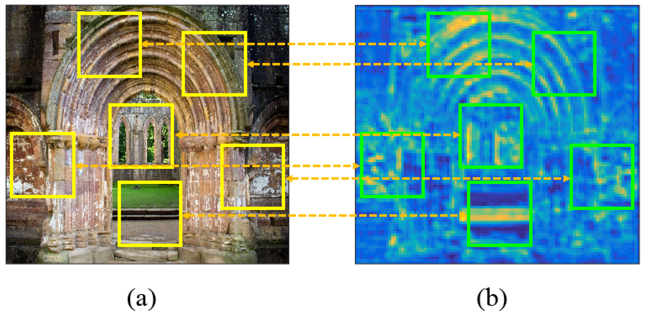
To discover the high-contrast and meaningful patches, we utilize the CSM to build the relationship between the original image and the corresponding convolutional activations. Concretely, we first transmit the original image to the VGG-19 network and obtain the CSM in the 4th convolutional layer, as shown in Figure 2b. From Figure 2b, we can see that those salient positions mainly distribute in the structural parts, and the values can reflect the importance of the local structure information. Hence, we propose the local weighted variance to reflect the contrast of the activation response at position in the 4th convolutional layer:
where defines a unit-volume Gaussian weighting window, and denote the activation response of the CSM at position in the 4th convolutional layer. Here, is the mean value of local activation responses:
To obtain the contrast in the activation-response region , we sum up all the local weighted variance within it:
The higher the value of is, the stronger the contrast of the activation-response region is. Hence, we take the value of as the criterion of high-contrast patch selection. The procedure of high-contrast patch selection is shown in Figure 2. Firstly, based on the , the high-contrast activation-response regions (the green rectangles in Figure 2b) in CSM are selected. Then, the selected high-contrast activation-response regions are mapped to the corresponding input image patches (the yellow rectangles in Figure 2a) so as to obtain the high-contrast patches. As a result, the useful patches are retained and the meaningless ones are abandoned.
2.3. Deep Activation Pooling
Suppose that F is a set of D-dimensional local features extracted from the K-selected high-contrast patches of pristine images, that is, , where is the D-dimensional feature vector of the k-th high-contrast patch. Based on these features, we learn a powerful opinion-unaware BIQA model. As shown in Figure 1d, in the training stage, we learn a PMVG model from the selected high-contrast patches. In the test stage, each selected high-contrast patch is fitted by a TMVG model, and then the TMVG model is compared with the PMVG model to obtain the local quality score of the patch. Finally, we utilize the proposed DAP to aggregate all the local quality scores to obtain the overall quality score. The specific procedure is listed as follows:
(a) We utilize a set of high-quality pristine images to train a PMVG model [19]. We first choose the CSM in the 4th convolutional layer of the VGG-19 network to select K high-contrast patches from the 90 pristine images using the high-contrast selection method mentioned in Section 2.2. Then, we extract the features for each selected high-contrast patch. Finally, based on the feature set F of the high-contrast patches, we apply the standard maximum likelihood estimation to learn a PMVG distribution:
where and represent the mean vector and the covariance matrix of F, respectively.
(b) Given a test image, we first resize the test image to the size of the pristine images, and then the high-contrast patch selection strategy is performed to obtain a set of patches. Each patch is represented as a feature vector, and each feature vector is fitted by a TMVG model. The learned TMVG model for the p-th patch where P is the number of the selected high-contrast patches of a test image) is denoted as . We compare the TMVG model of the p-th patch with the PMVG model to obtain the local quality score for the p-th patch. The procedure of learning the TMVG model for each patch is extremely costly. For simplicity, the quality score is computed using the following formula:
where is the feature vector of the p-th patch and is the covariance matrix computed from all the selected patches in the test image. Note that all the patches for one test image share the same .
(c) As we know, the contribution of each local quality score to the overall quality score is different. To emphasize the important patch scores and suppress the inessential ones, we propose the novel DAP method to obtain the overall quality score of the test image. Each activation response in the CSM describes a local part of the input image, and the high responses indicate the salient parts. We use the CSM in the 7th convolutional layer of the VGG-19 network to learn a weight for each local quality score. The weight of each local quality score is computed by adding all activation responses in the relevant activation-response region, as shown in the green rectangle of Figure 3. is the weight of the p-th patch and it is formulated as:
where represents the activation-response region and is the activation response of the CSM at position in the 7th convolutional layer. Let represent the weight set and be a set of local quality scores. The overall quality score of the test image can be obtained by:
The superiorities of our method lie in: (1) The proposed method could retain the primary structural and textual information and abandon the meaningless ones by performing the high-contrast selection; (2) the proposed DAP could automatically obtain the aggregating weights by learning the importance of local quality scores from the CSM, and therefore it overcomes the shortcomings of traditional average pooling and obtains more accurate overall quality score.
3. Experiments
In this section, we evaluate the effectiveness of the proposed method for opinion-unaware BIQA. We first introduce the evaluation protocols and databases in Section 3.1. We then describe the implementation details in Section 3.2. In Section 3.3, we compare the proposed opinion-unaware BIQA method with the representative inventive mechanisms. We validate the generalization ability of the proposed method in Section 3.4. To evaluate the proposed method more thoroughly, we also present the results on individual distortion types in Section 3.5. In Section 3.6, we study the influence of each kind of features on the final BIQA. Note that the results of blind/referenceless image spatial quality evaluator (BRISQUE), blind image integrity notator using DCT statistics (BLIINDS2), codebook representation for no-reference image assessment (CORNIA), natural image quality evaluator (NIQE) and integrated local natural image quality evaluator (IL-NIQE) are implemented by [19].
3.1. Evaluation Protocols and Databases
We utilize two indices in the experiments. The first index is the Spearman rank-order correlation coefficient (SRCC), which is between the subjective mean opinion scores (MOS) and the objective IQA scores. The second index is the Pearson linear correlation coefficient (PRCC), which is between the MOS and the objective IQA scores after a linear regression [23]. The SRCC and PRCC are used to evaluate the prediction monotonicity and consistency, respectively. The values of the SRCC and PRCC reflect the performance of the BIQA model. Typically, the higher the SRCC and PLCC values are, the better the BIQA model is.
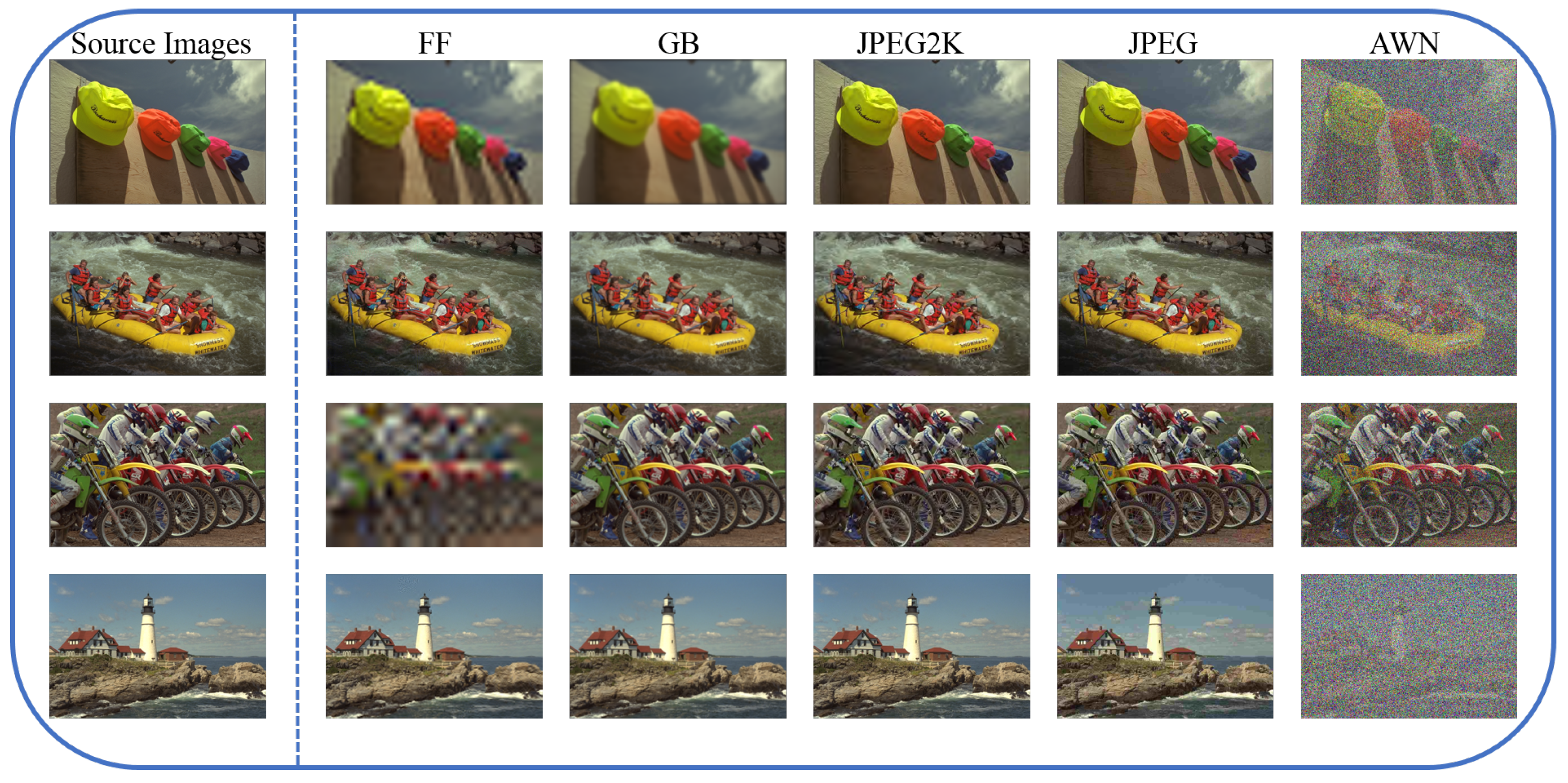
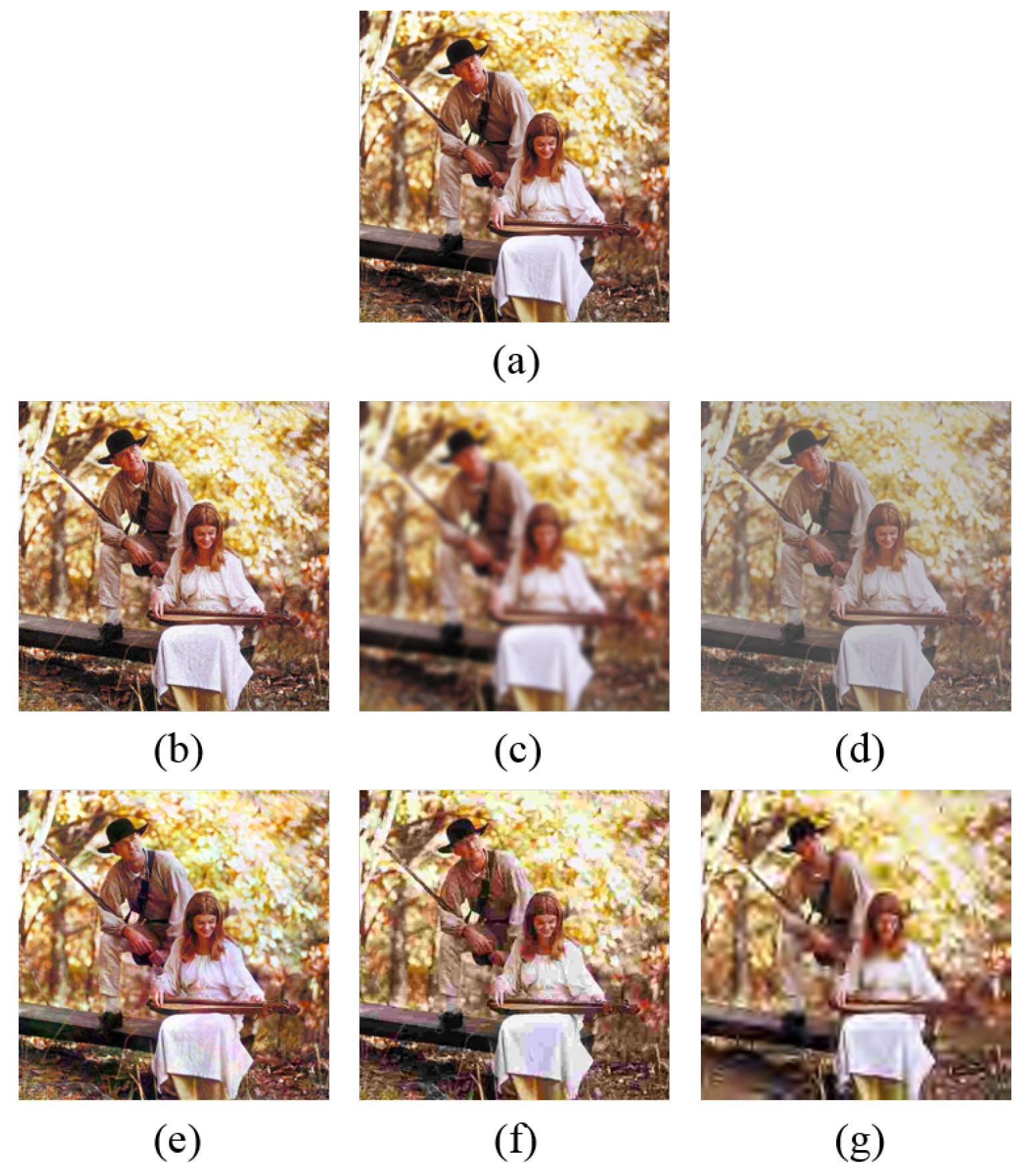
We utilize the SRCC and PRCC to evaluate the performance of the proposed method on two well-known IQA databases, the CSIQ [24] and LIVE [25] databases. The CSIQ database consists of 866 distorted images generated from 30 source images. Six types of distortions at five different levels are applied to the 30 source images, that is, additive white noise (AWN), Gaussian blur (GB), global contrast decrements (CTD), additive pink Gaussian noise (PGN), JPEG compression and JPEG2K compression. Some samples from the CSIQ database are shown in Figure 4. The LIVE database has 779 distorted images generated from 25 source images with five types of distortions at various levels. The distortions include simulated fast-fading Rayleigh channel (FF), GB, JPEG2K compression, JPEG compression and AWN. Figure 5 shows some images from the LIVE database.
3.2. Implementation Details
For fair comparison, we extract the same features as in [19] for each high-contrast patch. These features include the MSCN, MSCN products, gradients, log-Gabor filter responses and color-based features. As for a high-contrast patch, these five kinds of features are directly concatenated to obtain the feature vector of the patch, as shown in Figure 1c. The images are normalized into . The patch size and the percentage of the selected high-contrast patches for each image are empirically set to and 75%, respectively. The corresponding activation-response region sizes of the CSM in the 4th and the 7th convolutional layers are and , respectively. To verify the effectiveness, the proposed methods are compared with the representative inventive mechanisms, including three opinion-aware methods (BRISQUE [14], BLIINDS2 [26] and CORNIA [27]) and two opinion-unaware methods (NIQE [17] and IL-NIQE [19]). We also compare with HPSP+DAP, which indicates that we utilize the pristine images for selecting high-contrast patches as in [19], and the proposed DAP for learning pooling weights. The proposed method in this paper is denoted as HPSC+DAP, which means that we employ the CSM in 4th convolutional layer for high-contrast patch selection and the DAP for pooling weight learning.
In a CNN, the shallow convolutional layers usually contain structural and textural local features, while the deep convolutional layers usually contain high-level semantic information. In the opinion-unaware BIQA task, to discover the useful structural and textural information, we select the CSM in the shallow convolutional layers for high-contrast patch selection and pooling weight learning. We evaluate the performance of the proposed method when using CSM in different convolutional layers. For high-contrast patch selection, the index of convolutional layers varies from 3 to 8 with a step of 1, as shown in the rows of Table 2. For pooling weight learning, the index of convolutional layers also varies from 3 to 8 with a step of 1, as shown in the columns of Table 2. From Table 2, the experimental results indicate that the proposed method achieves the highest result when it utilizes the CSM in the 4th convolutional layer for selecting high-contrast patches and the CSM in the 7th convolutional layer for learning pooling weights.
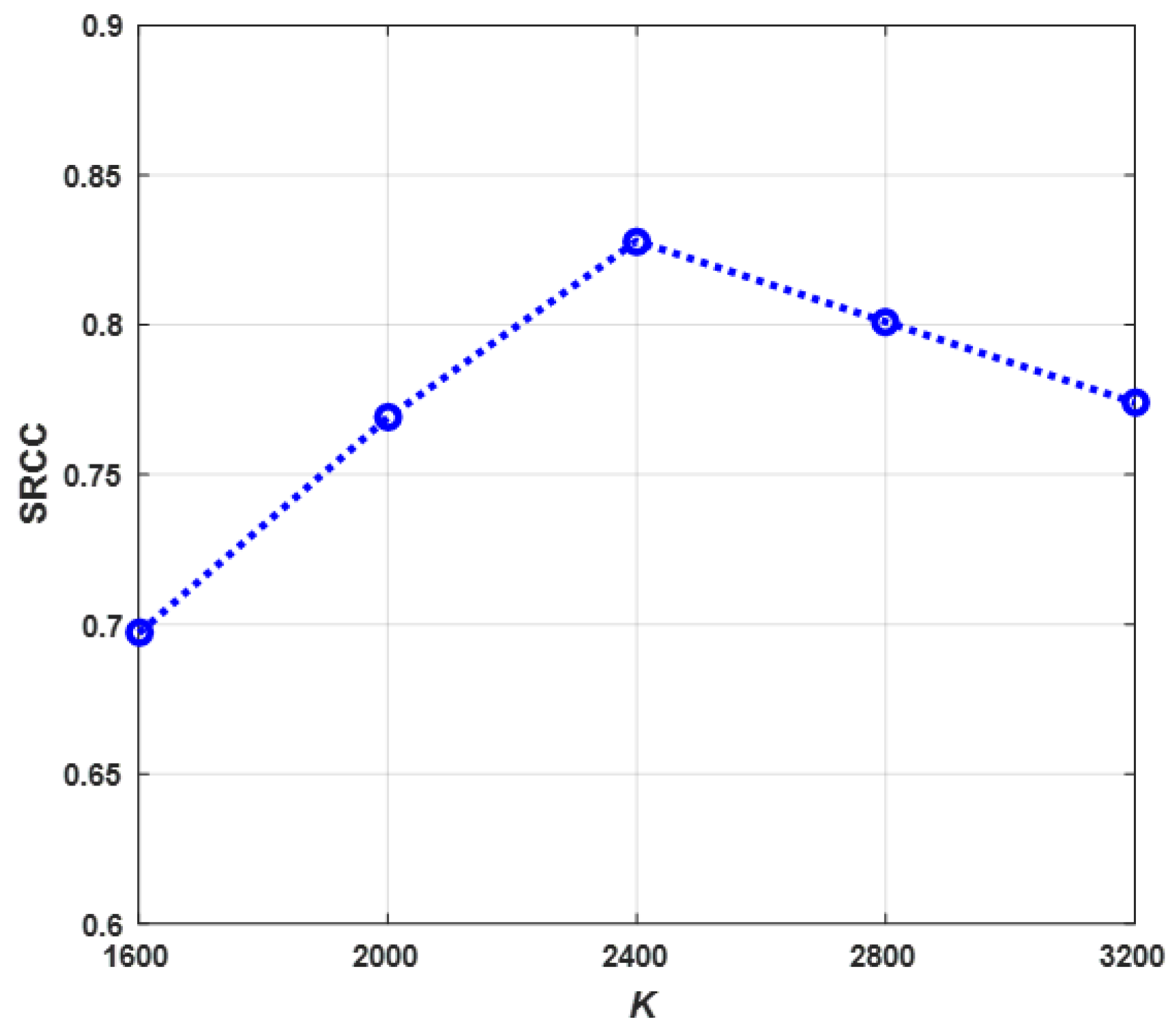
The number of the selected high-contrast activation-response regions K is an important parameter, and it affects the final results of BIQA. Hence, we investigate the influence of K. The range of K is from 1600 to 3200 with a step of 400, and the results on the CSIQ database are shown in Figure 6. The best performance is obtained when K is equal to 2400.
3.3. Performance Comparison with Other Methods
In Table 3, we compare the proposed method with three opinion-aware and two opinion-unaware methods on the CSIQ and LIVE databases. Since the opinion-aware methods learn regression models from distorted images, we partition each database into two subsets as in [19]. Specifically, distorted images correlated with 80% of the source images are used for training and the others are used for test. For fair comparison, we report the performance of the opinion-unaware methods on the partitioned test subset although they do not need training. From Table 3, we can draw several conclusions. First, the proposed HPSC+DAP is superior to all compared methods including opinion-aware methods and opinion-unaware methods. Second, compared with CORNIA, BRISQUE and BLIINDS2, which learn the regression model by using distortion images, the proposed HPSC+DAP achieves better performance without training on the LIVE database. Third, the proposed HPSC+DAP outperforms the SRCC and PRCC of the NIQE [17] by more than (0.2, 0.1) and (0.01, 0.01) on the CSIQ and LIVE databases, respectively. This is because the proposed HPSC+DAP utilizes the local TMVG model to capture local detail characteristics of distortion, while the NIQE only utilizes one global MVG model to describe an image. Fourth, the HPSP+DAP achieves better performance than IL-NIQE. The HPSP+DAP utilizes the DAP strategy to automatically emphasize the more important scores and suppress the less important ones, while the IL-NIQE method directly utilizes the average pooling to obtain the overall quality score. Fifth, the proposed HPSC+DAP obtains higher results than HPSP+DAP because the proposed HPSC+DAP utilizes the CSM in the convolutional layer, which could capture more meaningful information and remove the less important information, while the HPSP+DAP selects high-contrast patches on original images.
3.4. Performance on Generalization Ability
To validate the generalization ability of the proposed method, we compare it with other methods, and the results are shown in Table 4. In the experiment, the three opinion-aware methods, BRISQUE, BLIINDS2 and CORNIA, are trained on the LIVE database and tested on the CSIQ database. The learned opinion-unaware models, the NIQE, IL-NIQE and HPSC+DAP, are directly used to test the images on the CSIQ database. Compared with BRISQUE, BLIINDS2, CORNIA, NIQE and IL-NIQE, the proposed HPSC+DAP outperforms them by more than (0.2, 0.1), (0.2, 0.1), (0.1, 0.1), (0.2, 0.1) and (0.01, 0.01), respectively. The comparison results demonstrate that the proposed method possesses good generalization ability.
3.5. Performance on Individual Distortion Types
To evaluate the proposed method more thoroughly, we present the results on individual distortion types in Table 5. The experiments are conducted on the CSIQ and the LIVE databases. From Table 5, we can see that the proposed HPSC+DAP achieves the best results on the CTD, PGN, JPEG and JPEG2000 distortion types. On the distortion types of GB, FF and AWN, the proposed HPSC+DAP can also achieve competitive results. Hence, the proposed HPSC+DAP is powerful for opinion-unaware BIQA.
3.6. Influence of Each Kind of Features
We evaluate the performance of using four kinds of features on the CSIQ database for the proposed HPSC+DAP in order to understand the relative contribution of each kind of feature, and the results are listed in Table 6. From Table 6, we can see that each kind of feature positively contributes to the final BIQA, because using arbitrarily four kinds of features achieves lower performance than using all five kinds of features.
4. Conclusions
In this paper, we have proposed a novel method for opinion-unaware BIQA. The proposed method (1) can retain the primary structural and textural information and abandon the meaningless ones by utilizing the CSM for selecting high-contrast patches, and (2) can automatically emphasize the more important scores and suppress the less important ones by performing the DAP strategy. As a result, the proposed method obtains more accurate overall image quality scores. The proposed method has been validated on two well-known databases, that is, the CSIQ and LIVE databases, and the experimental results outperform the other previous methods in BIQA.
Acknowledgments
This work was supported by National Natural Science Foundation of China under Grant No. 61501327, No. 61711530240, Natural Science Foundation of Tianjin under Grant No. 17JCZDJC30600 and No. 15JCQNJC01700, the Fund of Tianjin Normal University under Grant No. 135202RC1703, the Open Projects Program of National Laboratory of Pattern Recognition under Grant No. 201700001 and and No. 201800002, the China Scholarship Council No. 201708120039 and No. 201708120040, and the NSFC-Royal Society Grant.
Author Contributions
All authors made significant contributions to the paper. Zhong Zhang and Hong Wang conceived, designed and performed the experiments, and wrote the paper; Shuang Liu performed the experiments and analyzed the data; Tariq S. Durrani provided the background knowledge of blind image quality assessment and reviewed the paper.
Conflicts of Interest
The authors declare no conflict of interest.
References
- Huang, Z.; Zhang, X.; Chen, L.; Zhu, Y.; An, F.; Wang, H.; Feng, S. A Hardware-efficient vector quantizer based on self-organizing map for high-speed image compression. Appl. Sci. 2017, 7, 1106. [Google Scholar] [CrossRef]
- Wang, Y.; Gau, Y.T.A.; Le, H.N.; Bergles, D.E.; Kang, J.U. Image analysis of dynamic brain activity based on gray distance compensation. Appl. Sci. 2017, 7, 858. [Google Scholar] [CrossRef]
- Kim, D.O.; Han, H.S.; Park, R.H. Gradient information-based image quality metric. IEEE Trans. Consum. Electron. 2010, 56. [Google Scholar] [CrossRef]
- Zhang, L.; Zhang, L.; Mou, X.; Zhang, D. FSIM: A feature similarity index for image quality assessment. IEEE Trans. Image Process. 2011, 20, 2378–2386. [Google Scholar] [CrossRef] [PubMed]
- Xue, W.; Zhang, L.; Mou, X.; Bovik, A.C. Gradient magnitude similarity deviation: A highly efficient perceptual image quality index. IEEE Trans. Image Process. 2014, 23, 684–695. [Google Scholar] [CrossRef] [PubMed]
- Pan, F.; Lin, X.; Rahardja, S.; Lin, W.; Ong, E.; Yao, S.; Yang, X. A locally adaptive algorithm for measuring blocking artifacts in images and videos. Signal Process Image 2004, 19, 499–506. [Google Scholar] [CrossRef]
- Liu, H.; Klomp, N.; Heynderickx, I. A no-reference metric for perceived ringing artifacts in images. IEEE Trans. Circuits Syst. Video Technol. 2010, 20, 529–539. [Google Scholar] [CrossRef]
- Liang, L.; Wang, S.; Chen, J.; Ma, S.; Zhao, D.; Gao, W. No-reference perceptual image quality metric using gradient profiles for JPEG2000. Signal Process Image 2010, 25, 502–516. [Google Scholar] [CrossRef]
- Bosse, S.; Maniry, D.; Müller, K.R.; Wiegand, T.; Samek, W. Deep neural networks for no-reference and full-reference image quality assessment. IEEE Trans. Image Process. 2018, 27, 206–219. [Google Scholar] [CrossRef] [PubMed]
- Moorthy, A.K.; Bovik, A.C. Blind image quality assessment: from natural scene statistics to perceptual quality. IEEE Trans. Image Process. 2011, 20, 3350–3364. [Google Scholar] [CrossRef] [PubMed]
- Tang, H.; Joshi, N.; Kapoor, A. Learning a blind measure of perceptual image quality. In Proceedings of the 2011 IEEE Conference on Computer Vision and Pattern Recognition, Colorado Springs, CO, USA, 20–25 June 2011; pp. 305–312. [Google Scholar]
- Li, C.; Bovik, A.C.; Wu, X. Blind image quality assessment using a general regression neural network. IEEE Trans. Neural Netw. 2011, 22, 793–799. [Google Scholar] [PubMed]
- Ma, K.; Liu, W.; Zhang, K.; Duanmu, Z.; Wang, Z.; Zuo, W. End-to-end blind image quality assessment using deep neural networks. IEEE Trans. Image Process. 2018, 27, 1202–1213. [Google Scholar] [CrossRef] [PubMed]
- Mittal, A.; Moorthy, A.K.; Bovik, A.C. No-reference image quality assessment in the spatial domain. IEEE Trans. Image Process. 2012, 21, 4695–4708. [Google Scholar] [CrossRef] [PubMed]
- Zhang, Y.; Chandler, D.M. No-reference image quality assessment based on log-derivative statistics of natural scenes. J. Electron. Imaging 2013, 22, 043025. [Google Scholar] [CrossRef]
- Xue, W.; Mou, X.; Zhang, L.; Bovik, A.C.; Feng, X. Blind image quality assessment using joint statistics of gradient magnitude and laplacian features. IEEE Trans. Image Process. 2014, 23, 4850–4862. [Google Scholar] [CrossRef] [PubMed]
- Mittal, A.; Soundararajan, R.; Bovik, A.C. Making a “completely blind” image quality analyzer. IEEE Signal Proc. Lett. 2013, 20, 209–212. [Google Scholar] [CrossRef]
- Xue, W.; Zhang, L.; Mou, X. Learning without human scores for blind image quality assessment. In Proceedings of the 2013 IEEE Conference on Computer Vision and Pattern Recognition, Portland, OR, USA, 23–28 June 2013; pp. 995–1002. [Google Scholar]
- Zhang, L.; Zhang, L.; Bovik, A.C. A feature-enriched completely blind image quality evaluator. IEEE Trans. Image Process. 2015, 24, 2579–2591. [Google Scholar] [CrossRef] [PubMed]
- Simonyan, K.; Zisserman, A. Very deep convolutional networks for large-scale image recognition. In Proceedings of the International Conference on Learning Representations (ICLR), San Diego, CA, USA, 7–9 May 2015. [Google Scholar]
- Wang, Y.; Shi, C.; Wang, C.; Xiao, B.; Qi, C. Multi-order co-occurrence activations encoded with Fisher Vector for scene character recognition. Pattern Recognit. Lett. 2017, 97, 69–76. [Google Scholar] [CrossRef]
- Cimpoi, M.; Maji, S.; Vedaldi, A. Deep filter banks for texture recognition and segmentation. In Proceedings of the 2015 IEEE Conference on Computer Vision and Pattern Recognition, Boston, MA, USA, 8–10 June 2015; pp. 3828–3836. [Google Scholar]
- Sheikh, H.R.; Sabir, M.F.; Bovik, A.C. A statistical evaluation of recent full reference image quality assessment algorithms. IEEE Trans. Image Process. 2006, 15, 3440–3451. [Google Scholar] [CrossRef] [PubMed]
- Larson, E.C.; Chandler, D.M. Most apparent distortion: full-reference image quality assessment and the role of strategy. J. Electron. Imaging 2010, 19, 011006. [Google Scholar]
- Sheikh, H.R.; Wang, Z.; Cormack, L.; Bovik, A.C. Live Image Quality Assessment Database Release 2. Available online: http://live.ece.utexas.edu./research/quality (accessed on 17 July 2007).
- Saad, M.A.; Bovik, A.C.; Charrier, C. Model-based blind image quality assessment using natural dct statistics. IEEE Trans. Image Process. 2011, 21, 3339–3352. [Google Scholar] [CrossRef] [PubMed]
- Ye, P.; Kumar, J.; Kang, L.; Doermann, D. Unsupervised feature learning framework for no-reference image quality assessment. In Proceedings of the 2011 IEEE Conference on Computer Vision and Pattern Recognition, Colorado Springs, CO, USA, 20–25 June 2011. [Google Scholar]
Figure 1.
The flowchart of the proposed method for BIQA. It is composed of (a) images and CSM, (b) selecting high-contrast patches, (c) building feature vectors, (d) learning MVG models, and (e) DAP is used to obtain the overall image quality score.
Figure 1.
The flowchart of the proposed method for BIQA. It is composed of (a) images and CSM, (b) selecting high-contrast patches, (c) building feature vectors, (d) learning MVG models, and (e) DAP is used to obtain the overall image quality score.
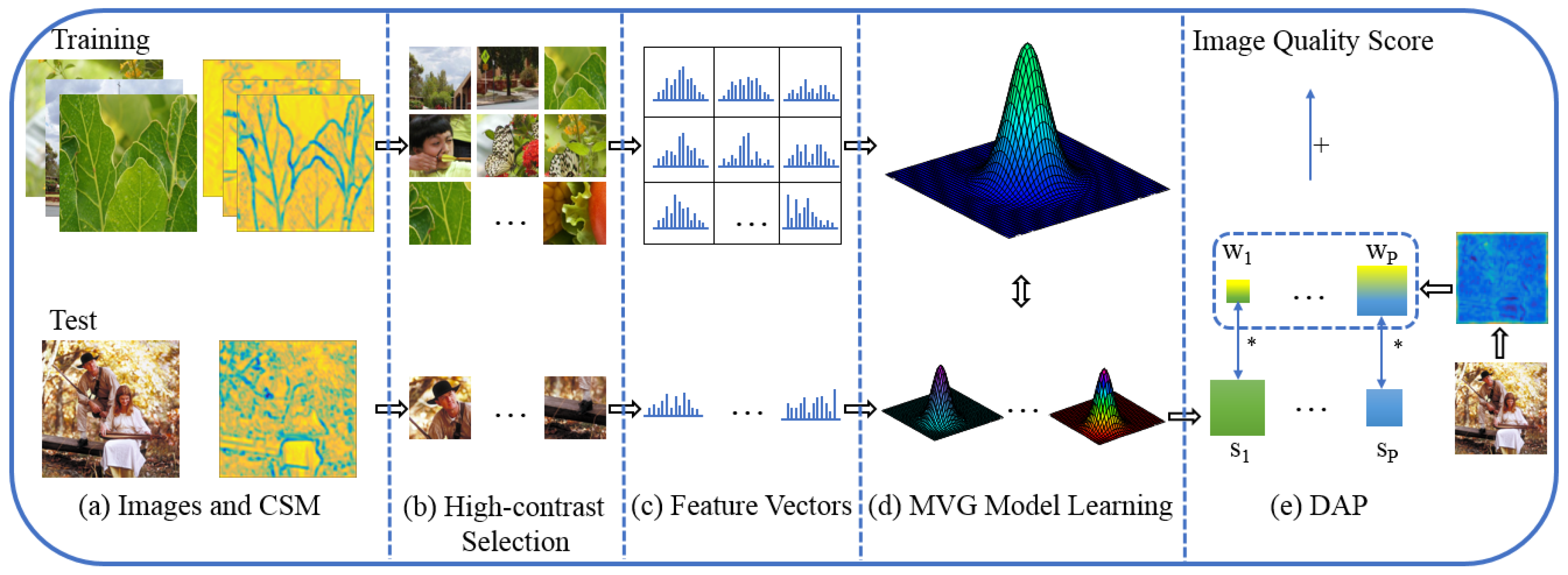
Figure 2.
(a) The input image; and (b) the CSM in 4th convolutional layer. In order to intuitively view the corresponding relationship between the input image and the CSM, we resize the CSM to the size of the input image.
Figure 2.
(a) The input image; and (b) the CSM in 4th convolutional layer. In order to intuitively view the corresponding relationship between the input image and the CSM, we resize the CSM to the size of the input image.

Figure 3.
Visualization of the DAP. (a) An image sample from the CSIQ database; (b) the CSM in the 7th convolutional layer of the VGG-19 network. The p-th yellow rectangle is used to obtain ( represents the local quality scores of the p-th patch), and the p-th green rectangle is used to compute ( is the corresponding weight of the p-th patch).
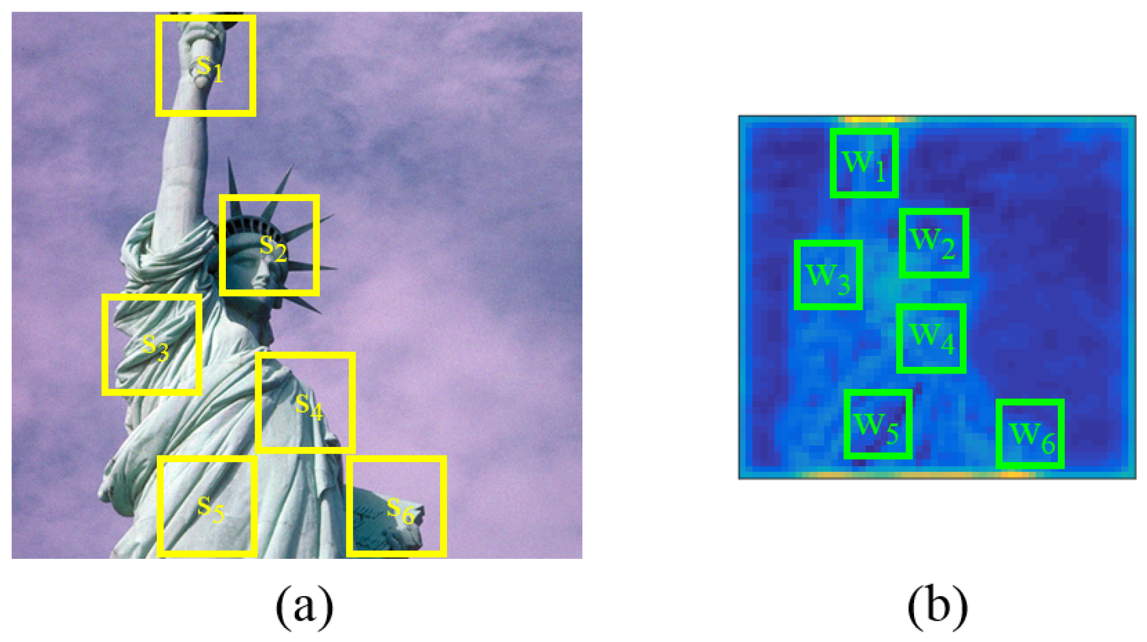
Figure 4.
Some samples from the CSIQ database.
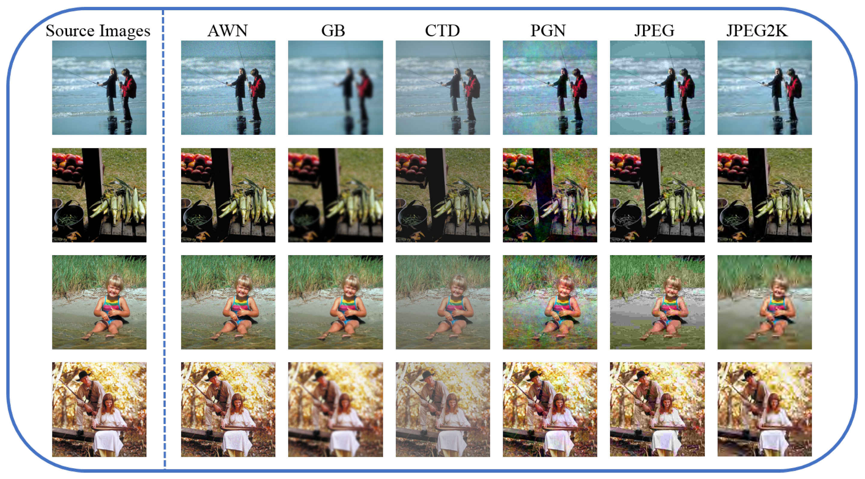
Figure 5.
Some samples from the LIVE database.

Figure 6.
The SRCC of the proposed HPSC+DAP under different K on the CSIQ database.

Figure 7.
(a) A reference image. Distorted images of (a): (b) AWN; (c) GB; (d) CTD; (e) PGN; (f) JPEG; (g) JPEG2K. The difference MOS of (b–g) are 0.325, 0.785, 0.352, 0.265, 0.586 and 0.805, respectively.
Figure 7.
(a) A reference image. Distorted images of (a): (b) AWN; (c) GB; (d) CTD; (e) PGN; (f) JPEG; (g) JPEG2K. The difference MOS of (b–g) are 0.325, 0.785, 0.352, 0.265, 0.586 and 0.805, respectively.


Table 1.
The architecture of VGG-19. The left part in “Building Blocks” indicates the size of receptive fields, and the right part indicates the number of filter banks.
Table 1.
The architecture of VGG-19. The left part in “Building Blocks” indicates the size of receptive fields, and the right part indicates the number of filter banks.
| Block Number | Convolution Stride | Spatial Padding | Building Blocks |
|---|---|---|---|
| Block1 | 1 | 1 | |
| Block2 | 1 | 1 | |
| Block3 | 1 | 1 | |
| Block4 | 1 | 1 | |
| Block5 | 1 | 1 | |
| FC-4096 | |||
| FC-4096 | |||
| FC-1000 | |||
Table 2.
The SRCC of the CSM in different convolutional layers on the CSIQ database. The best result is highlighted in bold.
Table 2.
The SRCC of the CSM in different convolutional layers on the CSIQ database. The best result is highlighted in bold.
| 3 | 4 | 5 | 6 | 7 | 8 | |
| 3 | 0.742 | 0.765 | 0.752 | 0.742 | 0.738 | 0.720 |
| 4 | 0.769 | 0.787 | 0.784 | 0.771 | 0.767 | 0.753 |
| 5 | 0.793 | 0.807 | 0.803 | 0.795 | 0.781 | 0.750 |
| 6 | 0.804 | 0.815 | 0.811 | 0.802 | 0.794 | 0.780 |
| 7 | 0.812 | 0.828 | 0.820 | 0.813 | 0.801 | 0.797 |
| 8 | 0.802 | 0.814 | 0.808 | 0.794 | 0.783 | 0.769 |
Table 3.
Evaluation results of different methods on the CSIQ and the LIVE databases. The best results are highlighted in bold.
Table 3.
Evaluation results of different methods on the CSIQ and the LIVE databases. The best results are highlighted in bold.
| BIQA Models | CSIQ | LIVE | ||
|---|---|---|---|---|
| SRCC | PRCC | SRCC | PRCC | |
| CORNIA [27] | 0.714 | 0.781 | 0.940 | 0.944 |
| BRISQUE [14] | 0.775 | 0.817 | 0.933 | 0.931 |
| BLIINDS2 [26] | 0.780 | 0.832 | 0.924 | 0.927 |
| NIQE [17] | 0.627 | 0.725 | 0.908 | 0.908 |
| IL-NIQE [19] | 0.822 | 0.865 | 0.902 | 0.906 |
| HPSP+DAP | 0.824 | 0.867 | 0.908 | 0.907 |
| Proposed HPSC+DAP | 0.829 | 0.871 | 0.919 | 0.921 |
Table 4.
Evaluation results of different methods when trained on the LIVE databases and tested on the CSIQ database. The best results are highlighted in bold.
Table 4.
Evaluation results of different methods when trained on the LIVE databases and tested on the CSIQ database. The best results are highlighted in bold.
| IQA Models | CSIQ | |
|---|---|---|
| SRCC | PRCC | |
| CORNIA [27] | 0.663 | 0.764 |
| BRISQUE [14] | 0.557 | 0.742 |
| BLIINDS2 [26] | 0.577 | 0.724 |
| NIQE [17] | 0.627 | 0.716 |
| IL-NIQE [19] | 0.815 | 0.854 |
| Proposed HPSC+DAP | 0.828 | 0.867 |
Table 5.
The SRCC of BIQA models on each individual distortion type. The best results are highlighted in bold.
Table 5.
The SRCC of BIQA models on each individual distortion type. The best results are highlighted in bold.
| Databases | Distortion Types | BRISQUE [14] | BLIINDS2 [26] | CORNIA [27] | NIQE [17] | IL-NIQE [19] | Proposed HPSC+DAP |
|---|---|---|---|---|---|---|---|
| CSIQ | AWN | 0.925 | 0.801 | 0.746 | 0.810 | 0.850 | 0.863 |
| GB | 0.903 | 0.892 | 0.917 | 0.895 | 0.858 | 0.869 | |
| CTD | 0.024 | 0.012 | 0.302 | 0.227 | 0.501 | 0.523 | |
| PGN | 0.253 | 0.379 | 0.420 | 0.299 | 0.874 | 0.891 | |
| JPEG | 0.909 | 0.900 | 0.908 | 0.882 | 0.899 | 0.916 | |
| JPEG2K | 0.867 | 0.895 | 0.914 | 0.907 | 0.906 | 0.921 | |
| LIVE | FF | - | - | - | 0.864 | 0.833 | 0.841 |
| GB | - | - | - | 0.933 | 0.915 | 0.929 | |
| JPEG2K | - | - | - | 0.919 | 0.894 | 0.920 | |
| JPEG | - | - | - | 0.941 | 0.942 | 0.947 | |
| AWN | - | - | - | 0.972 | 0.981 | 0.980 |
Table 6.
The SRCC of using different integrated features on the CSIQ databases. The “- X” means using four kinds of features other than “X”.
Table 6.
The SRCC of using different integrated features on the CSIQ databases. The “- X” means using four kinds of features other than “X”.
| Database | - MSCN | - MSCN Products | - Gradients | - Log-Gabor | - Color |
|---|---|---|---|---|---|
| CSIQ | 0.7713 | 0.7893 | 0.7462 | 0.7324 | 0.8048 |
© 2018 by the authors. Licensee MDPI, Basel, Switzerland. This article is an open access article distributed under the terms and conditions of the Creative Commons Attribution (CC BY) license (http://creativecommons.org/licenses/by/4.0/).
Share and Cite
MDPI and ACS Style
Zhang, Z.; Wang, H.; Liu, S.; Durrani, T.S. Deep Activation Pooling for Blind Image Quality Assessment. Appl. Sci. 2018, 8, 478. https://doi.org/10.3390/app8040478
AMA Style
Zhang Z, Wang H, Liu S, Durrani TS. Deep Activation Pooling for Blind Image Quality Assessment. Applied Sciences. 2018; 8(4):478. https://doi.org/10.3390/app8040478
Chicago/Turabian StyleZhang, Zhong, Hong Wang, Shuang Liu, and Tariq S. Durrani. 2018. "Deep Activation Pooling for Blind Image Quality Assessment" Applied Sciences 8, no. 4: 478. https://doi.org/10.3390/app8040478
Note that from the first issue of 2016, this journal uses article numbers instead of page numbers. See further details here.