Image Segmentation by Searching for Image Feature Density Peaks
by
 , ,
, ,
Zhe Sun
1, 
Meng Qi
1,
Jian Lian
2,
Weikuan Jia
1,*,
Wei Zou
3,
Yunlong He
1,
Hong Liu
1,4 and
Yuanjie Zheng
1,4,5,6,* 1
School of Information Science and Engineering, Shandong Normal University, Jinan 25030, China
2
Department of Electrical Engineering Information Technology, Shandong University of Science and Technology, Jinan 250031, China
3
Yantai Lanyoung Electronic Co., Ltd. Hangtian Road No. 101th, Block B 402# , Yantai 264003, China
4
Shandong Provincial Key Laboratory for Novel Distributed Computer Software Technology, Jinan 250300, China
5
Key Lab of Intelligent Computing & Information Security in Universities of Shandong, Shandong Normal University, Jinan 250300, China
6
Institute of Biomedical Sciences, Key Lab of Intelligent Information Processing, Shandong Normal University, Jinan 250300, China
*
Authors to whom correspondence should be addressed.
Appl. Sci. 2018, 8(6), 969; https://doi.org/10.3390/app8060969
Submission received: 14 May 2018
/
Revised: 2 June 2018
/
Accepted: 9 June 2018
/
Published: 13 June 2018
(This article belongs to the Special Issue Advanced Intelligent Imaging Technology)
Abstract
:Image segmentation attempts to classify the pixels of a digital image into multiple groups to facilitate subsequent image processing. It is an essential problem in many research areas such as computer vision and image processing application. A large number of techniques have been proposed for image segmentation. Among these techniques, the clustering-based segmentation algorithms occupy an extremely important position in this field. However, existing popular clustering schemes often depends on prior knowledge and threshold used in the clustering process, or lack of an automatic mechanism to find clustering centers. In this paper, we propose a novel image segmentation method by searching for image feature density peaks. We apply the clustering method to each superpixel in an input image and construct the final segmentation map according to the classification results of each pixel. Our method can give the number of clusters directly without prior knowledge, and the cluster centers can be recognized automatically without interference from noise. Experimental results validate the improved robustness and effectiveness of the proposed method.
1. Introduction
Image segmentation refers to partition an image into distinctive regions, where each region consists of pixels with similar attributes. The purpose of image segmentation is to simplify or change the representation of an image into some common features that are more meaningful and easier to analyze [1,2,3]. Over the past several decades, image segmentation has been widely used in diverse applications of computer vision and image processing, such as object detection [4], face recognition [5], image retrieval [6], and medical image analysis [7].
A large number of techniques and algorithms have been proposed for image segmentation. Color image segmentation of natural and outdoor scene is a well-studied problem due to its numerous applications in computer vision. Different methods have been already proposed in the state of the art based on different perspectives [8,9]. The most commonly used in image segmentation methods are listed roughly as follow: segmentation based on edge detection, region extraction, threshold method, and clustering techniques [10,11]. There also exists graph cut based method which performs image segmentation by using both edge and regional information [12]. Besides, segmentation may be also viewed as classification problem based on color and spatial features. In this regard, the rough set theory [13], which can extract the discriminative features from original data, has been applied to color image segmentation [14].
In particular, the K-means and fuzzy c-means (FCM) clustering are two of the most effective and popular algorithms in this field, which are carried out by classifying elements into different regions based on element similarity [15,16,17]. K-means clustering is a widely used technique with simple implementation and good convergence speed. This method aims to group pixels of a picture into K clusters, according to the similarity between a pair of data components [17]. In the segmentation process, K clustering centers are first determined, then this method intends to place them as far as possible away from each other for optimally clustering [1]. However, the clustering performance of this method depends heavily on prior knowledge, which may fail when data points described in the feature space are nonspherical clusters. Fuzzy clustering algorithm has been applied to many domains. This method superior to most hard clustering techniques in preserving original image information in the clustering process [18]. FCM is an unsupervised algorithm based on the idea that clustering the data points by minimizing the cost function iteratively and maximizing the distance between cluster centers [19,20,21]. However, the FCM algorithm is very sensitive to additive noise due to the lack of consideration of the image context, which lacks algorithm’s robustness to deal with image noise [22]. In addition, this method requires a large amount of calculation and often appears an over-segmentation phenomenon.
Alex et al. [15] propose a new clustering algorithm. It first defines two variables for each data point based on the nature of clustering centers. Then, a decision graph is designed to make the cluster centers isolated from other data points for clustering. However, the strategy in Alex et al. [15] still has drawbacks. For instance, the accuracy of the algorithm largely depends on the choice of threshold which is difficult to define effectively [23]. Besides, the cluster centers must be manually selected from the final decision graph generated by the algorithm.
In this paper, we propose a novel clustering-based method for image segmentation, which can automatically recognize the cluster centers by searching density peaks efficiently without defining the threshold. More specifically, we define a function to separate the clustering centers and other data points, change the way to calculate variables. In addition, this algorithm requires neither iteration nor prior knowledge, which can simply select the cluster centers and return the number of clusters.
2. Materials and Methods
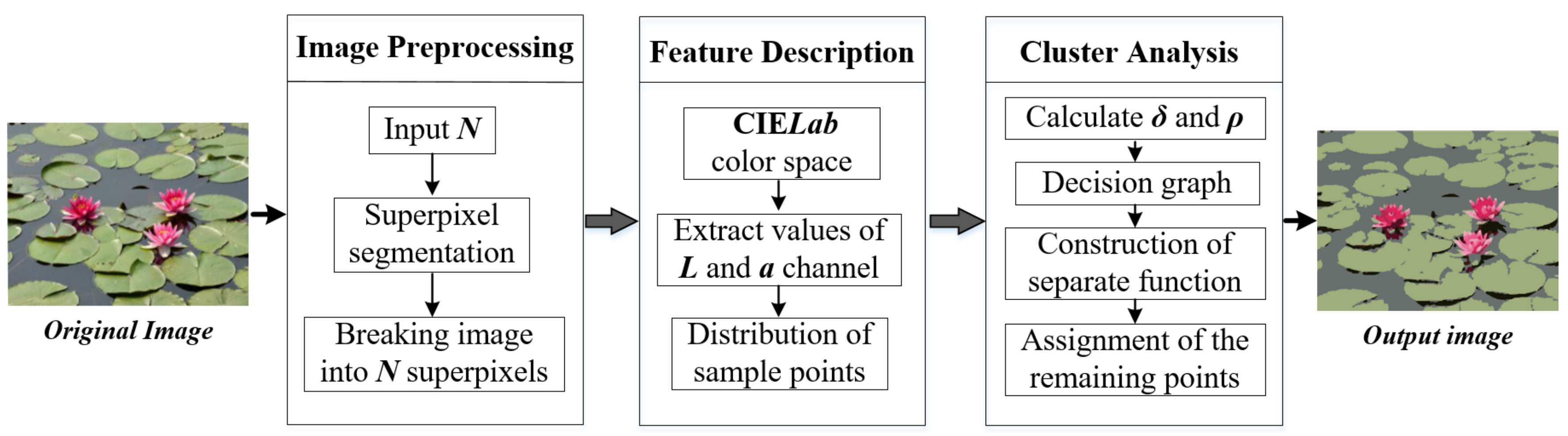
In this section, we present the technical details of our approach, which is carried out by searching for image feature density peaks. After image preprocessing and color feature extraction, the algorithm abstracts the color features into the sample distribution in cluster analysis. Then two variables are defined for each sample point separately: the local density of point i and its distance from the points with higher density. Finally, the cluster centers are recognized as points which have anomalously large values of and .
Figure 1 presents an overview of the approach. When dealing with image segmentation problems, what we need are often the picture’s feature information for each pixel, such as luminosity, color, contrast and other feature information, etc. So in the first place, we should extract this information, and store in an array or a vector digitally. Furthermore, it is crucial to find an applicable space to express these features for analyzing and quantifying in this space. Since the image size is relatively large, we need to preprocess it by using superpixel method for retaining the useful feature information and reducing data redundancy.
2.1. Superpixel Method for Image Preprocessing
The conventional segmentation approach will process each pixel one by one, which will cause a massive amount of data have trouble in analyzing, especially when the picture size is relatively large. In the present work, we use superpixel segmentation as an intermediate step to reduce the complexity of images from millions of pixels [24]. Superpixel segmentation aims to partition a picture into multiple homogeneous cells, we called superpixels, which has been widely applied to the picture analysis and simplification. Stutz et al. [25] comprehensively evaluated a variety of advanced superpixel algorithms in their studies. Among these algorithms, the simple linear iterative clustering (SLIC) can effectively adhere to image boundaries as well as or better than other schemes [26]. We employ this algorithm to divide the original image into a number of irregular blocks according to their similarity, which changes a pixel-level image into a district-level image. Each block is a perceptually consistent unit, and all pixels in a little superpixel region are most likely uniform in color. The different quantity of superpixels can be set according to the different size of the picture, and the values of the pixels contained in each superpixel region are the same. Hence each superpixel can be abstracted as a sample point. It is obviously that this way makes system requires less computation compared with other algorithms.
In this process, superpixel segmentation provides a more characteristic and significant representation easy to perceive of the digital image [27], most structures in the image are preserved. It is more helpful and meaningful for centralized processing of valid elements utilizing superpixel segmentation. There is very little loss in moving from the pixel-level map to the superpixel-level map. In the next task of image segmentation, superpixels are used as sample points for analysis. This method is illustrated by a simple example in Figure 2.
2.2. CIE Color Space for Image Feature Description
In the conventional color representation space, such as color space and color space, their channels contain not only color information but also luminosity information, which can not be extracted separately. In CIE space, because of its unique channel settings, luminosity features are stored in L channels alone, and color features are stored in a and b channels. They are independent of each other. Therefore, any operation to the image in the color space will not affect the hue. If luminosity and color features need to be extracted and adjusted, space will facilitate the operation. In addition, color space has a large range than space, which means that color information described in space can also be mapped in space, and it can make up for color distribution inhomogeneity in the other color space.
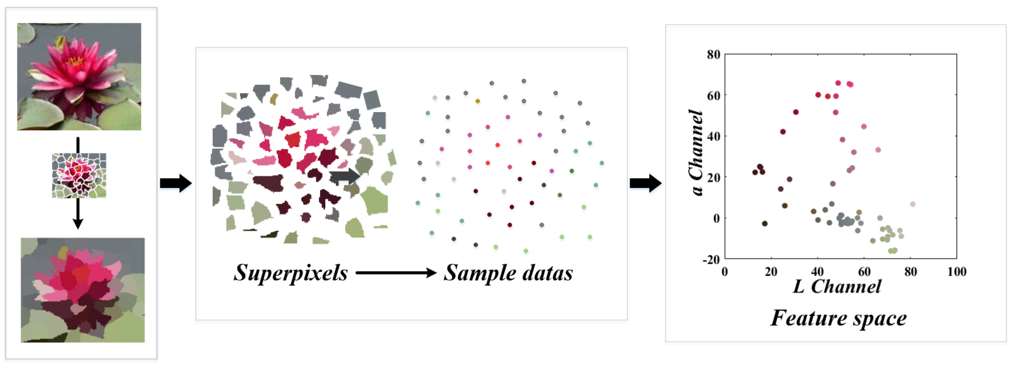
In this method, we choose the CIE color space, which consists of three channels for describing colors visible to human beings [28]. A method based on rough set for color channel selection proposed by Soumyabrata Dev et al. [14] provides ideas for the choice of color space in our work. Thus, in image segmentation, even only choose one color channel to analyze can we accomplish our task satisfactorily either. It also contributes to reducing the computation amount of the algorithm. After the superpixel segmentation is finished, we will use the planar space composed of L channel and a channel as the image feature space. With the distribution of sample points in the feature space, cluster analysis can be performed. More specifically, we take a fraction of Figure 2a and take it as an example, the above process is intuitively illustrated in Figure 3. Corresponding to the example of Figure 2, all the superpixels of this picture can be viewed as clustering sample points, and their distribution in the feature space is shown in Figure 4b.
2.3. Improvement of the Clustering Method
The novel clustering approach based on the assumption is that the cluster centers are surrounded by points with lower local density and have a relatively large distance from points with higher density [15]. The steps that required to complete this method are as follow:
For each point i, (N is the total number of superpixels) based on the basic assumption, there are only two quantities need to be computed: its distance from points of higher density, and its local density [15,23,29]. In the original clustering method, the local density is computed according to the following equation:
where
is the Euclidean distance between data point i and data point j, and is the cutoff distance. Actually, is decided based on the number of points that are closer than to point i. It’s obvious that the choice of has a huge impact on the algorithm if the value of is not appropriate, then the efficiency of the procedure will be greatly reduced. The solution of local density is an important parameter which indicates the sparseness of distribution of sample points and has a considerable influence on the final analysis results [30].
In our work, we proposed another way to compute local density without a cutoff distance. Kernel density estimation (KDE) [31] is the most commonly used density estimation method, which is a non-parametric way to estimate the probability density function of a random variable. Let us define an multivariable independent sample , whose distribution is drawn from our superpixels distribution in the feature space. In other words, the values of the sample points in the L channel and a channel are respectively stored in x and y. We intend to fit the shape of samples’ probability density function , its kernel density estimator is:
where K is kernel which is a non-negative function integrates into one. is bandwidth, which is also called window, it is a smoothing parameter whose choice will strongly influence the estimation results [32].
The kernel density estimation is to use a smooth peak function we called ’kernel’ to fit the observed data points, so as to simulate the true probability distribution curve. Kernel density estimate has many types of kernel, the Gaussian kernel function is one of the most commonly used among them, so we apply it to figure out local density .
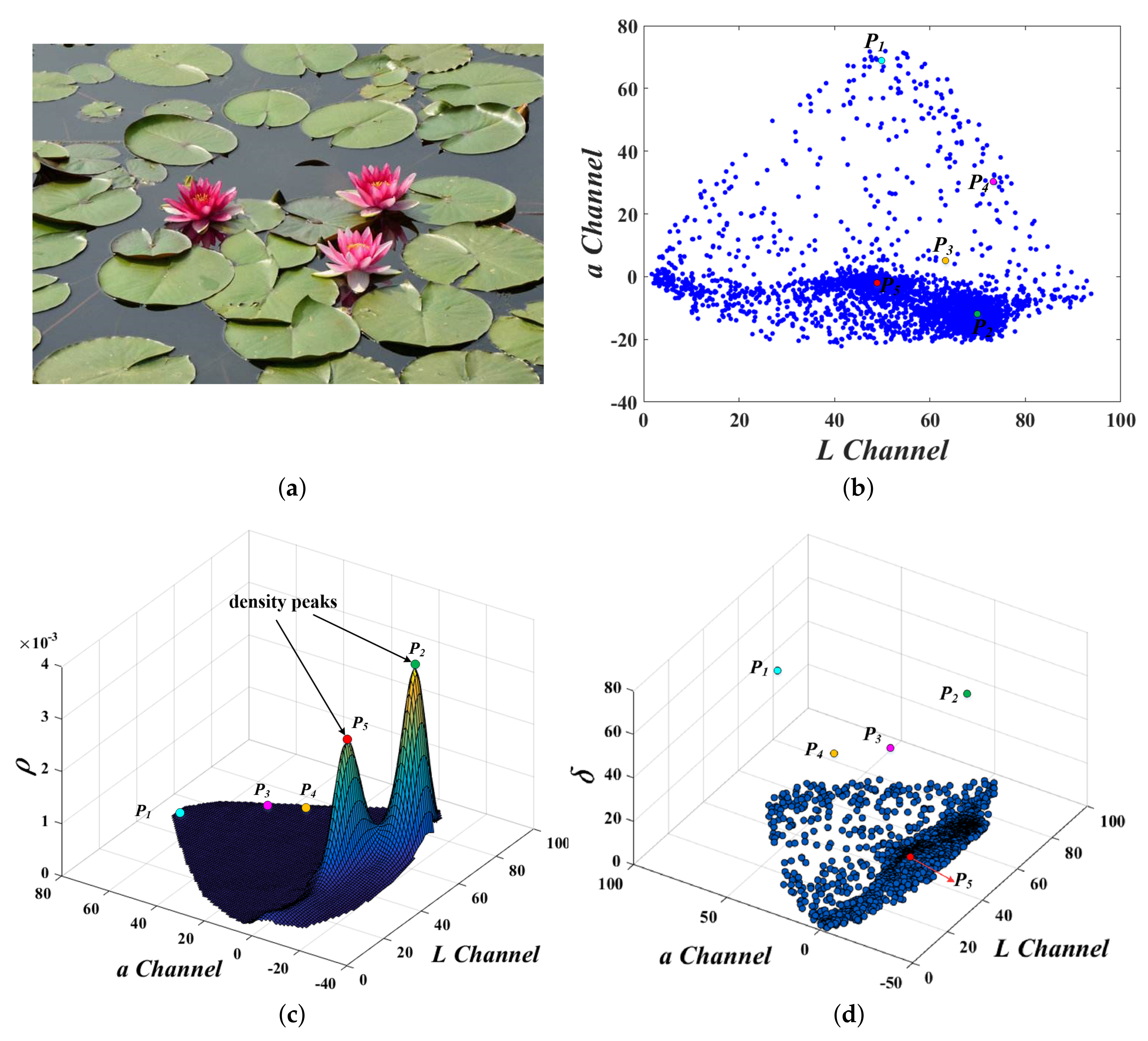
In this method, we used the kernel approach described in [16]. And we can see the 3-dimensional density estimation result clearly in Figure 4a. In addition to the following calculations, the density values and function shape also provide grounds for roughly estimating the location of the cluster centers and more comprehensively classifying sample points.
After we figure out the local density , the distance can be computed by choosing the minimum distance between the point i and any other points with higher density, we take the maximum distance between data points as its . The distance for each point i is defined as:
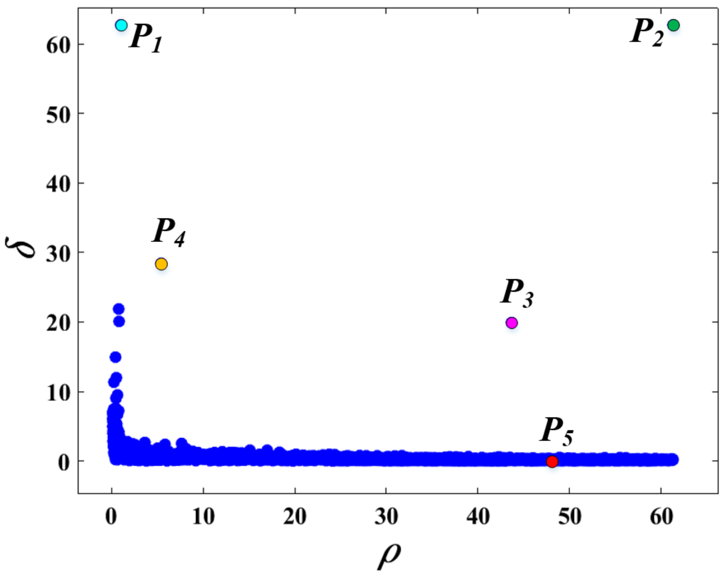
We can find an important characteristic of the cluster centers based on the results of and . The cluster centers are the points with high local density and a relatively high distance between other points with higher density, i.e. . Based on this assumption, we construct a new graph containing both the and in it, called decision graph. Figure 5 shows the decision graph, which is represented based on the both the local density and distance adopted in our method. The decision graph is designed to represent the core nature of cluster centers, horizontal axis and vertical axis respectively pull the cluster center upward and rightward, so that the cluster centers stand out.
The KDE searches the density peaks in the probability estimate function plot (Figure 4c) accurately, and in Figure 4d it is not difficult to find that there are only a few points with a large value of . Comprehensive and values, when their values of some sample points are both large, these points are most likely cluster centers. However, the final result in [15] still needs to be manually selected, which is considerably affected by human factors, different options will lead to entirely different segmentation results.
2.4. Adaptive Selection of Cluster Centers
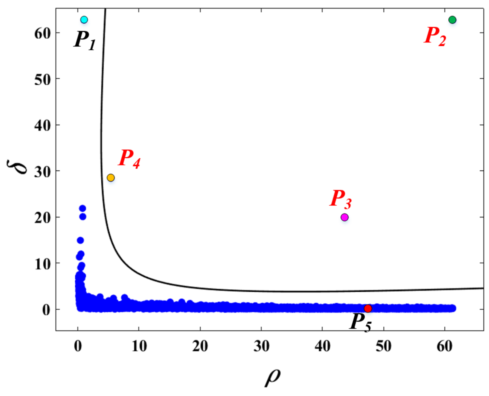
Due to the difficulty of solving the above problem, a separate function is found to assist in picking the cluster centers automatically. The measure of functions is based on the method in [33] as following:
k is a constant determined by experience, which will affect the accuracy of the algorithm to some extent. In Section 3, the exact k value and its influence on the accuracy will be discussed in detail. The points are considered as cluster centers when . Thus, the separate function can achieve the separation between cluster centers and other sample points. Therefore, the decision graph in Figure 5 can be redrawn as follows:
As shown in Figure 6, the points to the right of the curve are considered as the cluster centers. And after the cluster centers have been found, the remaining data points will be assigned to the same clusters as its nearest neighbors of higher density. Once a point is assigned to a cluster, the information regarding the classification is updated immediately, this procedure continues until no valid candidates are left to be assigned [8]. We define the of a point i as follows:
For each point, we check its candidacy firstly. This helps us to filter out the points which are not valid candidates to be analyzed and hence reduces the computational time. This step is shown in Algorithm 1.
| Algorithm 1 Assignment of remaining points |
Input: cluster centers ; the local density set and distance set for all superpixels computed from the original image.
|
Marking each pixel points with its cluster number, and the cluster number of each pixel data is the cluster number of the superpixel area to which the point belongs. And fill all pixel points with the mean color of the clusters they are belonging to. Then achieving the final segmentation based on the numbers marked through the last step, as shown in Figure 7.
3. Experiment
3.1. Data and Experimental Setting
We employed the Berkeley segmentation database (BSDS300) for evaluation of our segmentation scheme. The BSDS300 database consists of 300 natural images, each with multiple ground truth segmentations provided by different individuals. This database contains a variety of content, including landscapes, animals, buildings, and portraits, makes it a challenge for any segmentation algorithm. In addition, it has found wide acceptance as a public benchmark for testing image segmentation algorithms [34,35]. In this paper, the entire BSDS300 database is first employed to investigate the effect of several user-defined parameters and evaluate the performance of our method compared to other schemes. Then, we divided the database into 7 different subsets according to specific content in order to further evaluate the segmentation performance in preserving the salient features of the input images. The evaluation details will be discussion in Section 3.2. All of our experiments are performed on PC with Intel CoreTM i7-6700 CPU with a frequency of 3.40 GHz and 8 GB of RAM under MS Windows 10.
Following the previous works [22,36], we adopt the commonly used Probabilistic Rand index (PRI) [34,37] to measure the results of image segmentation for each image within the dataset. PRI was initially introduced for measuring the similarity between two data clusterings. It is now widely used for the comparison of segmentation algorithms using multiple ground truth images. PRI operates by comparing the compatibility of assignments between pairs of elements in the clusters. Its value between test and ground truth segmentations is computed by the sum of the number of pairs of pixels that have the same label in test S and ground truth segmentations G, and those that have different labels, divided by the total number of the couple of pixels [34]. Specifically, given a set of ground-truth segmentations , the PRI is defined as:
where is the event that pixels i and j have the same label and its probability. T is the total number of pixel pairs. We employ the sample mean to estimate , Equation (10) amounts to averaging the PRI among different ground-truth segmentations. The PRI has been reported to suffer from a small dynamic range [38,39], and PRI values across images and algorithms are often similar. In [38], this drawback is addressed by normalization with empirical estimation of its expected value.
3.2. Evaluation
We carried out a series of experiments to validate the usefulness of the output of our segmentation method. We first ran our algorithm on the entire database to investigate the effect of several user-defined parameters and to empirically choose an optimal value for these parameters. Then, we evaluate the proposed method by comparing the qualitative & quantitative performance of our method with state-of-the-art schemes. Both the quantitative and qualitative results demonstrated that our method could successfully improve segmentation accuracy.
3.2.1. Effects of Parameters
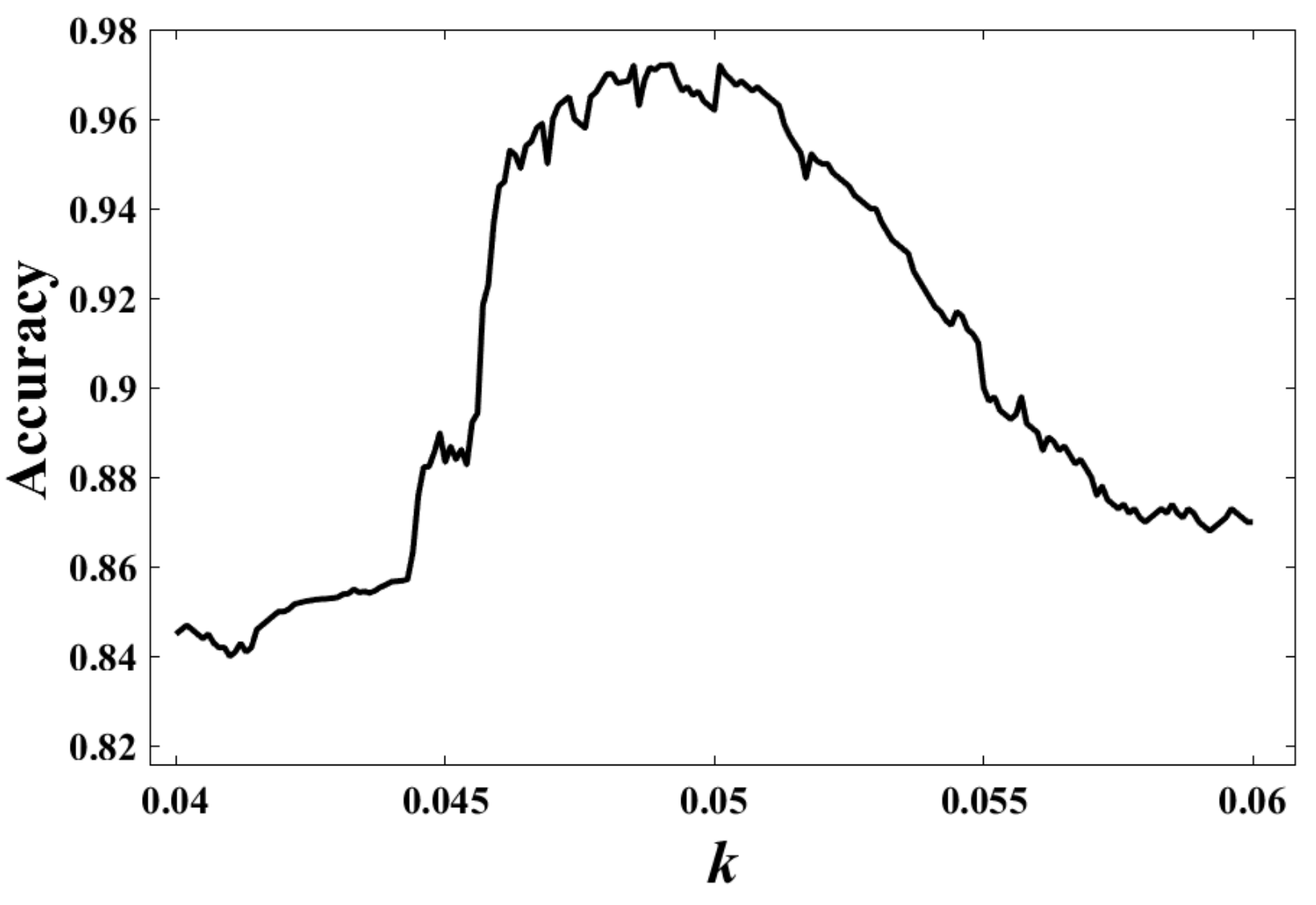
Ronneberger2015UNetConvolutionalIn our algorithm, there are practically only two parameters to control, h (bandwidth in Equation (3)) and k (constant in Equation (6)). h is a parameter which basically determines the bandwidth of smoothing window and have a clear impact on the performance. Typically, an estimate with smaller value of h might provide a better estimate to the empirical cumulative distribution function. We performed our algorithms with varied value of h, and we found that the segmentation accuracy tends to be stable when when h varied from 0.5 to 1.5. Afterwards, we compare the performance when under fixed value of k. We observed that the segmentation accuracy achieves the best when . Thus we empirically set h to be in our experiment for keeping a stable performance. Moreover, we found that the accuracy tends to be stable when k takes values between and after running our algorithm for a certain number of times. For , we found that it also has a clear impact on the segmentation performance, as shown in Figure 8, where the accuracy indicates the ratio of the total correctly classified pixels. In addition, the accuracy tends to be stable when k is 0.0462 and 0.0515, and it reaches the peak of 0.0972 when .
3.2.2. Quantitative Evaluation
To quantitatively evaluate our algorithm, we use PRI to compare the performance of the proposed method with other schemes. We first perform all methods on the entire database by following their optimal settings to do the comparison experiments. The average values of PRI computed on 300 images of BSD300 dataset are shown in 8th raw of Table 1, in which our scheme achieves the highest value. In addition, in order to further evaluate the classification performance of our method, we divided the databased into 7 subsets based on different content and characteristics appearing on images. Then the PRI counts the fraction of pairs of pixels whose labels are consistent between the computed segmentation and the ground truth, averaging across multiple ground truth segmentations to account for scale variation in human perception [40]. The PRI values for all types of images are shown in the first 7 raws of Table 1. As noted in this Table, the sensitivity of the proposed method is best with PRI = 0.897, which are also the highest value among the other two methods, and only 0.002 behind the K-means method [41] on the image 122048 type. Moreover, we have shown the average computation time for all methods, which indicates that our method can be carried out with less computational cost.
3.2.3. Qualitative Evaluation
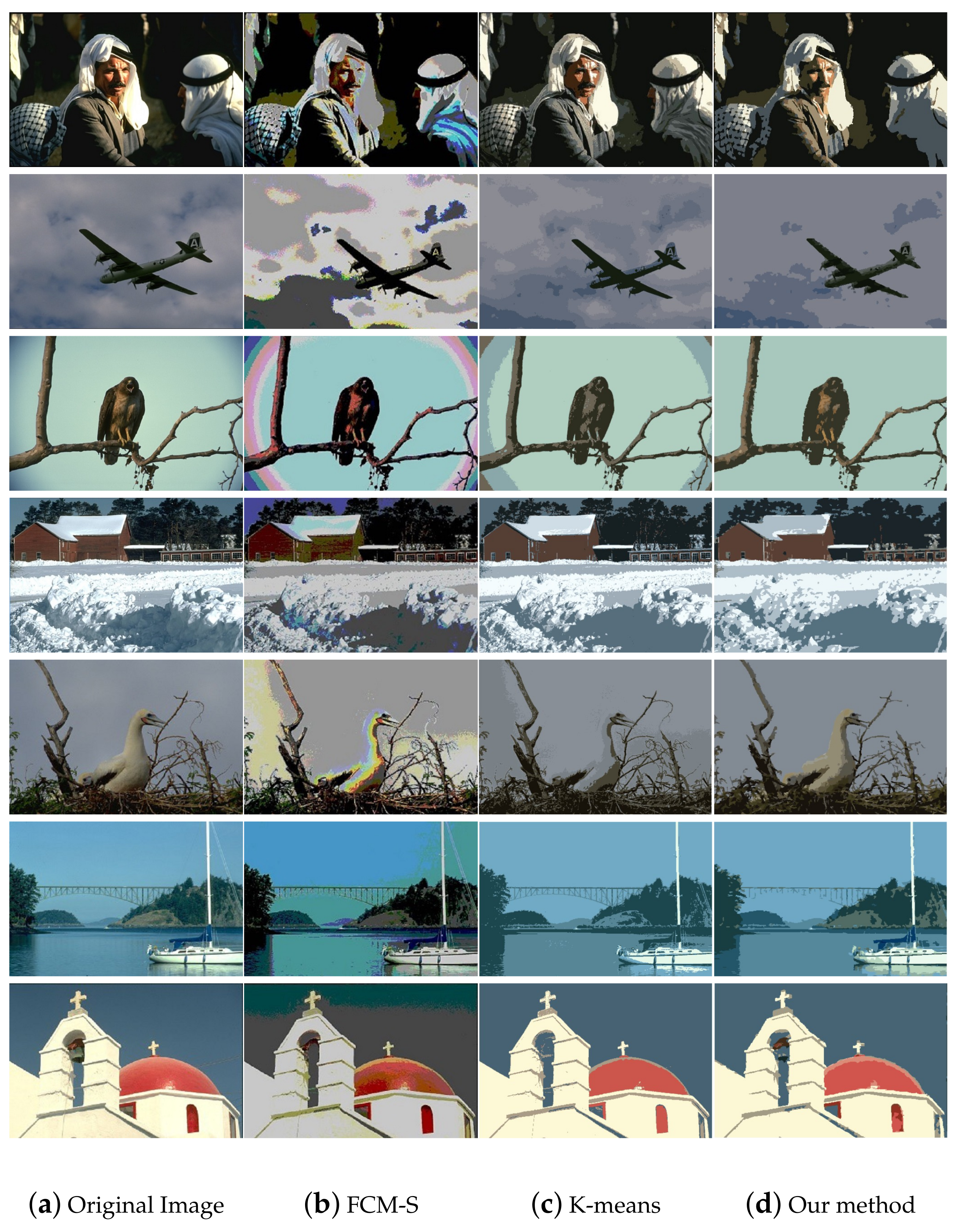
To prove the effectiveness of the proposed method, we compare our method with existing segmentation methods on the Berkeley datasets: BSDS300. We compute the results of our method on entire datasets, and then the results of FCM-S and K-means are computed by following the optimal settings in the previous work [41,42], respectively. Figure 9 shows the qualitative results of 7 images, with each one is randomly selected from one of 7 image types (corresponding to first 7 rows of Table 1). These results suggest that our method can achieve superior performance in preserving the salient features of the input images due to its excellent accuracy of pixel classification. For example, from Figure 9, it can clearly be observed that there are considerable number of pixels in the white kerchief or human face (1st row), body of the bird (5th row), and the church clock (end row) are falsely clustered as background or the part of the other objects. Comparing with the other two segmentation approaches, the proposed scheme accomplishes the segmentation requests by avoiding these classification errors through reasonably classifying these pixels. Moreover, as we can see in the 3rd row of Figure 9, there is an obvious intensity inhomogeneity occurring around the image. By contrast, the proposed scheme outperforms the FCM-S and K-means by producing more homogeneous background.
4. Discussion
In this paper, we proposed a new image segmentation method which does not require a priori knowledge and a large amount of computation. This method is based on the assumption that a cluster center is surrounded by its neighbors with lower density, and the data with a higher density than the cluster center must be far from it. The decision graph is designed to take variables into comprehensive consideration, and a separate function is automatically defined to select cluster centers, and thus the algorithm can figure out the most appropriate number of clusters according to the actual situation of different pictures in the case of unsupervised.
Image segmentation problem is challenging, many issues still need to be resolved. Our method is based on the clustering model in [15], but more of an automatic method and does not define the threshold. Superpixel segmentation methods are used to make an image preprocessing to reduce the computational complexity, and regardless of the size of the input image. Moreover, the computation time of the algorithm can always be maintained within a very reasonable range. Experiment results indicate that our method is more effective and more stable compared to state-of-the-art clustering methods.
We still have some challenges, such as the number of superpixel areas still needs more evidence to determine to avoid segmentation results are not meticulous enough, and it is also closely related to the runtime.
Author Contributions
Methodology, Z.S. and Y.Z.; Data curation, Z.S. and J.L.; Validation, Z.S. and Y.H.; Resources, H.L. and W.Z.; Writing—Original Draft Preparation, Z.S.; Writing—Review & Editing, M.Q. and W.J.
Funding
National Nature Science Foundation of China (No. 61572300); Natural Science Foundation of Shandong Province in China (ZR2017BC013, ZR2014FM001); Taishan Scholar Program of Shandong Province of China (No. TSHW201502038).
Acknowledgments
This work is supported by the National Nature Science Foundation of China (No. 61572300); Natural Science Foundation of Shandong Province in China (ZR2017BC013, ZR2014FM001); Taishan Scholar Program of Shandong Province of China (No. TSHW201502038).
Conflicts of Interest
The authors declare no conflict of interest.
References
- Chen, Z.; Qi, Z.; Meng, F.; Cui, L.; Shi, Y. Image segmentation via improving clustering algorithms with density and distance. Procedia Comput. Sci. 2015, 55, 1015–1022. [Google Scholar] [CrossRef]
- Shapiro, L.; Stockman, G.C. Computer Vision; Prentice Hall: Englewood Cliffs, NJ, USA, 2001. [Google Scholar]
- Barghout, L.; Lee, L. Perceptual Information Processing System. US Patent App. 10/618,543, 11 July 2003. [Google Scholar]
- Zhuang, H.; Low, K.S.; Yau, W.Y. Multichannel pulse-coupled-neural-network-based color image segmentation for object detection. IEEE Trans. Ind. Electron. 2012, 59, 3299–3308. [Google Scholar] [CrossRef]
- Kim, D.S.; Jeon, I.J.; Lee, S.Y.; Rhee, P.K.; Chung, D.J. Embedded face recognition based on fast genetic algorithm for intelligent digital photography. IEEE Trans. Ind. Electron. 2006, 52, 726–734. [Google Scholar]
- Kumar, V.D.; Thomas, T. Clustering of invariance improved legendre moment descriptor for content based image retrieval. In Proceedings of the 2008 International Conference on Signal Processing, Communications and Networking (ICSCN’08), Chennai, India, 4–6 January 2008; pp. 323–327. [Google Scholar]
- Pham, D.L.; Xu, C.; Prince, J.L. Current methods in medical image segmentation. Ann. Rev. Biomed. Eng. 2000, 2, 315–337. [Google Scholar] [CrossRef] [PubMed]
- Md. Abul Hasnat, O.A.; Tremeau, A. Joint Color-Spatial-Directional Clustering and Region Merging (JCSD-RM) for Unsupervised RGB-D Image Segmentation; IEEE Computer Society: Washington, DC, USA, 2016; pp. 2255–2268. [Google Scholar]
- Angelova, A.; Zhu, S. Efficient object detection and segmentation for fine-grained recognition. In Proceedings of the IEEE Conference on Computer Vision and Pattern Recognition, Portland, OR, USA, 23–28 June 2013; pp. 811–818. [Google Scholar]
- Al Aghbari, Z.; Al-Haj, R. Hill-manipulation: An effective algorithm for color image segmentation. Image Vis. Comput. 2006, 24, 894–903. [Google Scholar] [CrossRef]
- Cheng, H.; Li, J. Fuzzy homogeneity and scale-space approach to color image segmentation. Pattern Recogn. 2003, 36, 1545–1562. [Google Scholar] [CrossRef]
- Boykov, Y.Y.; Jolly, M.P. Interactive graph cuts for optimal boundary & region segmentation of objects in ND images. In Proceedings of the Eighth IEEE International Conference on Computer Vision (ICCV 2001), Vancouver, BC, Canada, 7–14 July 2001; Volume 1, pp. 105–112. [Google Scholar]
- Pawlak, Z. Rough Sets: Theoretical Aspects of Reasoning about Data; Springer Science & Business Media: New York, NY, USA, 2012; Volume 9. [Google Scholar]
- Dev, S.; Savoy, F.M.; Lee, Y.H.; Winkler, S. Rough-set-based color channel selection. IEEE Geosci. Remote Sens. Lett. 2017, 14, 52–56. [Google Scholar] [CrossRef]
- Rodriguez, A.; Laio, A. Clustering by fast search and find of density peaks. Science 2014, 344, 1492–1496. [Google Scholar] [CrossRef] [PubMed]
- Wang, J.; Wang, H. A study of 3D model similarity based on surface bipartite graph matching. Eng. Comput. 2017, 34, 174–188. [Google Scholar] [CrossRef]
- Kandwal, R.; Kumar, A.; Bhargava, S. Existing Image Segmentation Techniques. Int. J. Adv. Res. Comput. Sci. Softw. Eng. 2014, 4, 153–156. [Google Scholar]
- Zhang, H.; Wu, Q.J.; Nguyen, T.M. Image segmentation by a robust generalized fuzzy c-means algorithm. In Proceedings of the 2013 20th IEEE International Conference on Image Processing (ICIP), Melbourne, VIC, Australia, 15–18 September 2013; pp. 4024–4028. [Google Scholar]
- Naik, D.; Shah, P. A review on image segmentation clustering algorithms. Int. J. Comput. Sci. Inform. Technol. 2014, 5, 3289–3293. [Google Scholar]
- Zhang, H.; Lu, J. Creating ensembles of classifiers via fuzzy clustering and deflection. Fuzzy Sets Syst. 2010, 161, 1790–1802. [Google Scholar] [CrossRef]
- Tan, K.S.; Lim, W.H.; Isa, N.A.M. Novel initialization scheme for Fuzzy C-Means algorithm on color image segmentation. Appl. Soft Comput. 2013, 13, 1832–1852. [Google Scholar] [CrossRef]
- Zheng, Y.; Jeon, B.; Xu, D.; Wu, Q.; Zhang, H. Image segmentation by generalized hierarchical fuzzy C-means algorithm. J. Intell. Fuzzy Syst. 2015, 28, 961–973. [Google Scholar]
- Wang, S.; Wang, D.; Li, C.; Li, Y. Comment on “Clustering by Fast Search and Find of Density Peaks”. arXiv, 2015; arXiv:1501.04267. [Google Scholar]
- Mehra, J.; Neeru, N. A brief review: Super-pixel based image segmentation methods. Imp. J. Interdiscip. Res. 2016, 2, 8–12. [Google Scholar]
- Stutz, D.; Hermans, A.; Leibe, B. Superpixels: An evaluation of the state-of-the-art. Comput. Vis. Image Underst. 2018, 166, 1–27. [Google Scholar] [CrossRef] [Green Version]
- Achanta, R.; Shaji, A.; Smith, K.; Lucchi, A.; Fua, P.; Süsstrunk, S. SLIC superpixels compared to state-of-the-art superpixel methods. IEEE Trans. Pattern Anal. Mach. Intell. 2012, 34, 2274–2282. [Google Scholar] [CrossRef] [PubMed]
- Bowman, A.W.; Azzalini, A. Applied Smoothing Techniques for Data Analysis: The Kernel Approach with S-Plus Illustrations; OUP: Oxford, UK, 1997; Volume 18. [Google Scholar]
- Yan, Y.; Shen, Y.; Li, S. Unsupervised color-texture image segmentation based on a new clustering method. In Proceedings of the 2009 International Conference on New Trends in Information and Service Science (NISS’09), Beijing, China, 30 June–2 July 2009; pp. 784–787. [Google Scholar]
- Yheng, Y.; Lin, S.; Kambhamettu, C.; Yu, J.; Kang, S.B. Single-Image Vignetting Correction. IEEE Trans. Pattern Anal. Mach. Intell. 2009, 31, 2243–2256. [Google Scholar]
- Luo, C.; Zhang, X.; Zheng, Y. Chaotic Evolution of Prisoner’s Dilemma Game with Volunteering on Interdependent Networks. Commun. Nonlinear Sci. Numer. Simul. 2017, 47, 407–415. [Google Scholar] [CrossRef]
- Botev, Z.I.; Grotowski, J.F.; Kroese, D.P. Kernel Density Estimation Via Diffusio. Ann. Stat. 2010, 38, 2916–2957. [Google Scholar] [CrossRef]
- Sheather, S.J.; Jones, M.C. A Reliable Data-Based Bandwidth Selection Method for Kernel Density Estimation. J. R. Stat. Soc. 1991, 53, 683–690. [Google Scholar]
- Rosten, E.; Drummond, T. Machine Learning for High-Speed Corner Detection. In Computer Vision—ECCV 2006; Springer: Berlin/Heidelberg, Germany, 2006; pp. 430–443. [Google Scholar]
- Arbelaez, P.; Maire, M.; Fowlkes, C.; Malik, J. Contour detection and hierarchical image segmentation. IEEE Trans. Pattern Anal. Mach. Intell. 2011, 33, 898–916. [Google Scholar] [CrossRef] [PubMed]
- Donoser, M.; Urschler, M.; Hirzer, M.; Bischof, H. Saliency driven total variation segmentation. In Proceedings of the 2009 IEEE 12th International Conference on Computer Vision, Kyoto, Japan, 29 September–2 October 2009; pp. 817–824. [Google Scholar]
- Unnikrishnan, R.; Hebert, M. Measures of similarity. In Proceedings of the Seventh IEEE Workshops on Application of Computer Vision (WACV/MOTIONS’05), Washington, DC, USA, 5–7 January 2005; Volume 1, p. 394. [Google Scholar]
- Rand, W.M. Objective criteria for the evaluation of clustering methods. J. Am. Stat. Assoc. 1971, 66, 846–850. [Google Scholar] [CrossRef]
- Unnikrishnan, R.; Pantofaru, C.; Hebert, M. Toward objective evaluation of image segmentation algorithms. IEEE Trans. Pattern Anal. Mach. Intell. 2007, 29, 929–944. [Google Scholar] [CrossRef] [PubMed]
- Yang, A.Y.; Wright, J.; Ma, Y.; Sastry, S.S. Unsupervised segmentation of natural images via lossy data compression. Comput. Vis. Image Underst. 2008, 110, 212–225. [Google Scholar] [CrossRef] [Green Version]
- Rohit, S. Comparitive Analysis of Image Segmentation Techniques. Int. J. Adv. Res. Comput. Eng. Technol. 2013, 2, 2615–2619. [Google Scholar]
- Arthur, D.; Vassilvitskii, S. k-means++: The advantages of careful seeding. In Proceedings of the Eighteenth Annual ACM-SIAM Symposium on Discrete Algorithms, New Orleans, LA, USA, 7–9 January 2007; Society for Industrial and Applied Mathematics: Philadelphia, PA, USA, 2007; pp. 1027–1035. [Google Scholar]
- Chen, S.; Zhang, D. Robust image segmentation using FCM with spatial constraints based on new kernel-induced distance measure. IEEE Trans. Syst. Man Cybern. Part B (Cybern.) 2004, 34, 1907–1916. [Google Scholar] [CrossRef]
Figure 1.
Overview of our image segmentation framework.

Figure 2.
The process of superpixel pre-segmentation. (a) The original image. (b) We partition the original image into multiple homogeneous. (c) The superpixel level map. Calculating the average of the color features for each superpixel region and use that value to replace the pixel values for all points in the region. In this process, not only can maximize the retention of the effective information but can drop some unnecessary noise, the complexity of the calculation will be greatly reduced.

Figure 3.
The flowchart of Section 2.1 and Section 2.2. The small image is an interesting region selected from the original image, and this interesting region is divided into 62 superpixels. We consider each superpixel as a sample point and represent them in feature space.
Figure 3.
The flowchart of Section 2.1 and Section 2.2. The small image is an interesting region selected from the original image, and this interesting region is divided into 62 superpixels. We consider each superpixel as a sample point and represent them in feature space.

Figure 4.
(a) Original image. (b) The 2-d color feature space for all sample points from image (a), which is represented through the strategy illustrated in Figure 3. (c) Local density for sample points, which are shown as 3D shaded surface plot of the probability density function. (d) Distributions of discrete distance for 3D condition, which are computed by using Equation (5).

Figure 5.
The decision graph, which is represented based on the both the local density and distance used in our method.
Figure 5.
The decision graph, which is represented based on the both the local density and distance used in our method.

Figure 6.
Separate Function Decision Graph. The letters of final cluster centers are marked by red color.
Figure 6.
Separate Function Decision Graph. The letters of final cluster centers are marked by red color.

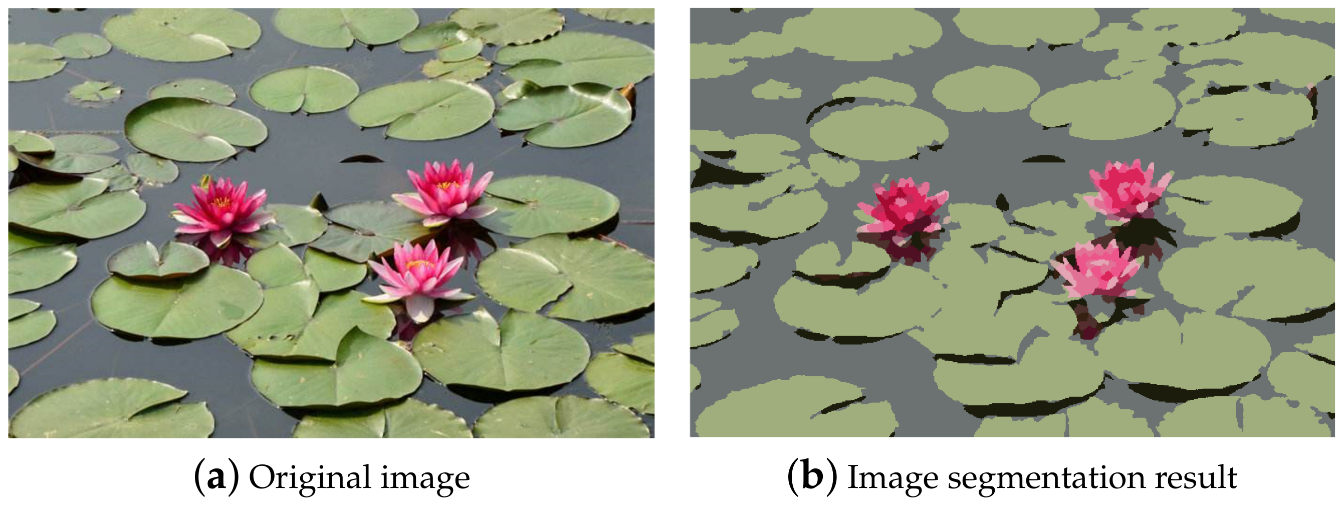
Figure 7.
The segmentation result (a) by our method on the original picture (b).

Figure 8.
Performance with different parameter values, k is an constant between 0.04 and 0.06.

Figure 9.
Results for different segmentation algorithms based on clustering. (a) Original image (b) FCM-S based segmentation (c) K-means based segmentation (d) The method we proposed.
Figure 9.
Results for different segmentation algorithms based on clustering. (a) Original image (b) FCM-S based segmentation (c) K-means based segmentation (d) The method we proposed.


Table 1.
Comparison of different method for Berkeley image dataset, Probabilistic Rand Index (PRI).
| Image Type | FCM-S | K-Means | Our Method |
|---|---|---|---|
| human | 0.510 | 0.674 | 0.672 |
| transport | 0.503 | 0.563 | 0.592 |
| intensity inhomogeneity | 0.608 | 0.653 | 0.651 |
| building 1 | 0.715 | 0.694 | 0.712 |
| animal | 0.816 | 0.803 | 0.837 |
| landscape | 0.704 | 0.783 | 0.818 |
| building 2 | 0.819 | 0.885 | 0.897 |
| Mean | 0.668 | 0.722 | 0.740 |
| average computation time | 5.782s | 4.237s | 5.331s |
© 2018 by the authors. Licensee MDPI, Basel, Switzerland. This article is an open access article distributed under the terms and conditions of the Creative Commons Attribution (CC BY) license (http://creativecommons.org/licenses/by/4.0/).
Share and Cite
MDPI and ACS Style
Sun, Z.; Qi, M.; Lian, J.; Jia, W.; Zou, W.; He, Y.; Liu, H.; Zheng, Y. Image Segmentation by Searching for Image Feature Density Peaks. Appl. Sci. 2018, 8, 969. https://doi.org/10.3390/app8060969
AMA Style
Sun Z, Qi M, Lian J, Jia W, Zou W, He Y, Liu H, Zheng Y. Image Segmentation by Searching for Image Feature Density Peaks. Applied Sciences. 2018; 8(6):969. https://doi.org/10.3390/app8060969
Chicago/Turabian StyleSun, Zhe, Meng Qi, Jian Lian, Weikuan Jia, Wei Zou, Yunlong He, Hong Liu, and Yuanjie Zheng. 2018. "Image Segmentation by Searching for Image Feature Density Peaks" Applied Sciences 8, no. 6: 969. https://doi.org/10.3390/app8060969
Note that from the first issue of 2016, this journal uses article numbers instead of page numbers. See further details here.