Signal Source Localization of Multiple Robots Using an Event-Triggered Communication Scheme

Abstract

This paper deals with the problem of signal source localization using a group of autonomous robots by designing and analyzing a decision-control approach with an event-triggered communication scheme. The proposed decision-control approach includes two levels: a decision level and a control level. In the decision level, a particle filter is used to estimate the possible positions of the signal source. The estimated position of the signal source gradually approaches the real position of signal source with the movement of robots. In the control level, a consensus controller is proposed to control multiple robots to seek a signal source based on the estimated signal source position. At the same time, an event-triggered communication scheme is designed such that the burden of communication can be lightened. Finally, simulation and experimental results show the effectiveness of the proposed decision-control approach with the event-triggered communication scheme for the problem of signal source localization.

1. Introduction

Signal source localization can be widely found in nature and society [1,2,3,4,5,6,7]. For example, some bacteria are able to find chemical or light sources through the perception of the external environment [1]. Moreover, reproducing this kind of behavior in mobile robots can be used to perform some complex missions such as monitoring environments [2,3,8,9], searching and rescuing victims [10], and so on. How to deal with the problem of signal source localization has attracted increasing interest from scientists and engineers and involves two aspects of study. One aspect is to estimate the possible positions of signal sources, while the other aspect is to control robots to locate signal sources based on the estimated positions [2,3]. For a single robot, some approaches have been proposed for the problem of signal source localization. For example, in [11], the SPSA (Simultaneous Perturbation Stochastic Approximation) method was designed to control the mobile robot to locate a signal source. In [12,13], the extremum seeking technique, originally developed for adaptive control, was also applied in signal source localization. In [14], a source probability estimation approach was proposed to control the robot to locate the signal source by using the information on signal strength and direction angle. However, the aforementioned approaches need the robot to take more time to collect measurements at different locations. Moreover, some search trajectories generated by these approaches are usually unnecessary.

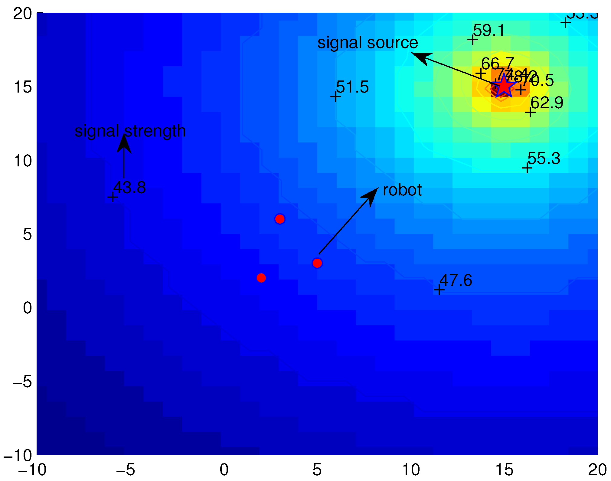
Compared with the single robot, due to the wide detection range and simultaneous sampling, multi-robot systems have received much attention for the problem of signal source localization (see Figure 1) [15,16,17,18,19,20,21]. Usually, the integrated gradient estimation of the signal strength distribution is a common method to estimate the possible position of the signal source, which means that multiple robots simultaneously obtain the measurements at different locations and give the movement direction such that some unnecessary trajectories are neglected [18,22,23]. For example, in [18], Nikolay approximated the signal strength gradient at the formation centroid via a Finite-Difference (FD) scheme and proposed distributed control strategies for localizing a noisy signal source. In [2], Lu used a radial basis function network to model the search environment and guided the robots to move toward the signal source based on gradient information provided by the environment model. Correspondingly, some cooperative control approaches [2,3] have been developed in terms of consensus control theory [23,24,25,26]. Moreover, the idea of cooperative control is further extended to deal with the management of crisis situations [27]. For example, in [28], Garca-Magariño proposed a coordination approach among citizens for locating the sources of problems by using peer-to-peer communication and a global map.

It should be pointed out that two issues may arise in the aforementioned approaches for the problem of signal source localization. One issue is that the gradient estimation method is easily influenced by noises so as to fall into local optima [29]. For this issue, a particle filter approach can be employed to deal with the uncertainty problem raised by noises. The other issue is that the communication resources in multi-robot systems are constrained, i.e., each robot has a limited communication bandwidth. For this issue, an event-triggered scheme can be used to reduce communication times for each robot. It is worth mentioning that there are some event-triggered rules that have been proposed [2,30,31,32] for multi-robot systems. However, these kinds of event-triggered rules only save computational resources. For multi-robot systems, continuous communication schemes still need to be used to hold system stability. In order to reduce both computational resources and communication burden, several event-triggered communication schemes have been designed [33,34,35,36] such that communication resources can be saved. However, there is no result available for the problem of signal source localization, which can combine the particle filter approach with the cooperative control approach with an event-triggered communication scheme. One challenge is how to design event-triggered communication rules based on the given cooperative control approach. The other challenge is how to derive stability conditions for the multi-robot systems with the proposed cooperative control approach using an event-triggered communication rule. Therefore, how to develop the decision-control approach for the problem of signal source localization in the face of the aforementioned challenges motivates the present study.

The proposed decision-control approach has two advantages. One advantage is that the use of the event-triggered communication scheme can effectively decrease the communication times and lower the updating frequency of control input such that the communication and chip resources are saved. The other advantage is that the detection information from the multi-robot system can be well used to estimate the position of the signal source by the particle filter and cooperative controller. The remainder of this paper is arranged as follows. In Section 2, we will briefly give the preliminaries on the dynamics of mobile robots and communication topologies. In Section 3, we will use a particle filter to estimate the position of the signal source and propose a cooperative control approach with an event-triggered communication scheme to coordinate the mobile robots to locate the signal source. In Section 4 and Section 5, we will show the effectiveness of the proposed decision-control approach with the event-triggered communication scheme by simulation and experimental results, respectively. Finally, we will conclude this paper in Section 6.

2. Preliminaries

2.1. Dynamics of Mobile Robots

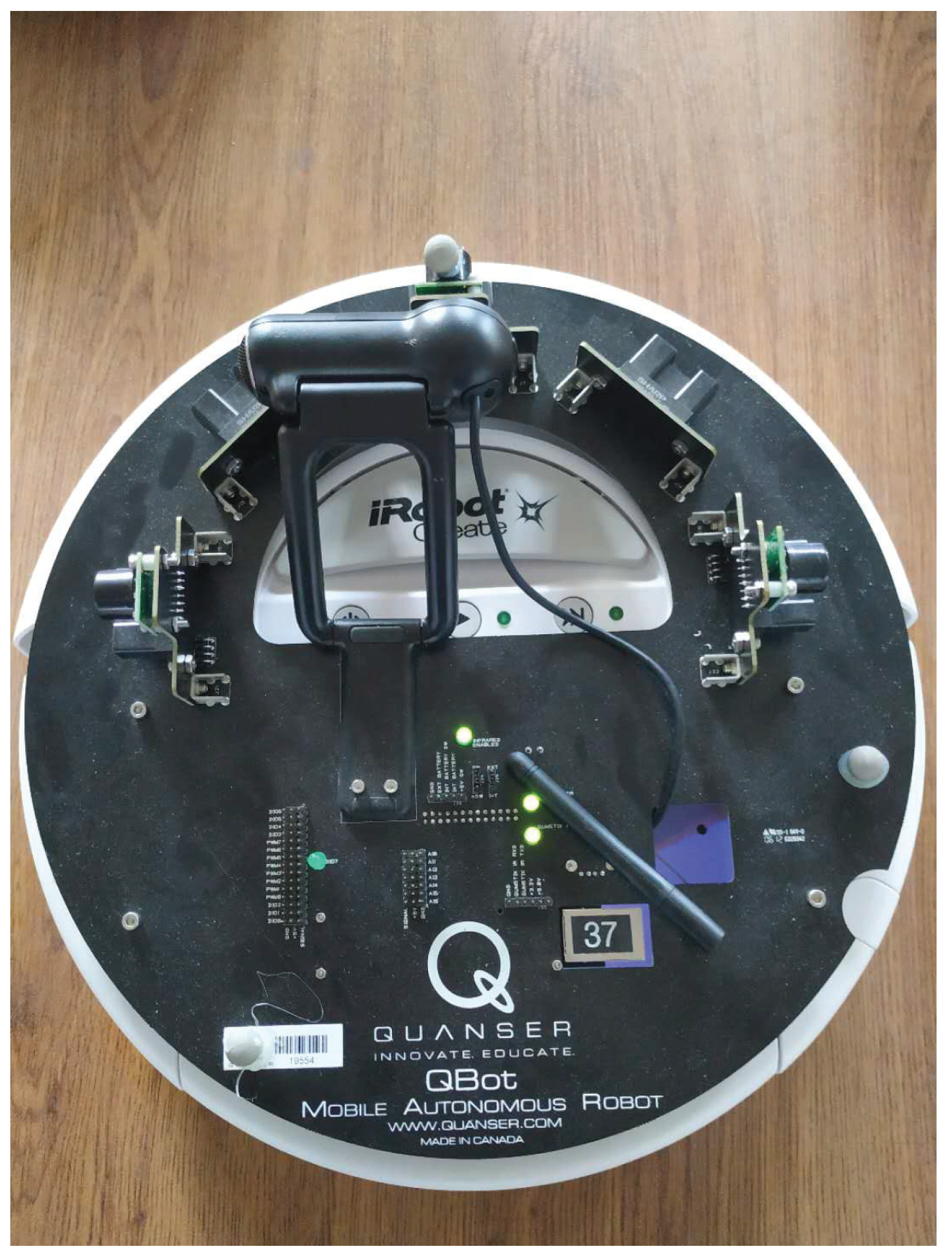
For mobile robots, such as Qbot in Figure 2, the dynamics can be described by:

$$\begin{array}{ccc}\hfill \left(\begin{array}{c}{\dot{r}}_{xi}\\ {\dot{r}}_{yi}\\ {\dot{\theta }}_i\\ {\dot{\nu }}_i\\ {\dot{\omega }}_i\end{array}\right)& =& \left(\begin{array}{c}{\nu }_i\cos {\theta }_i\\ {\nu }_i\sin {\theta }_i\\ {\omega }_i\\ 0\\ 0\end{array}\right)+\left(\begin{array}{cc}0& 0\\ 0& 0\\ 0& 0\\ \frac{1}{m_i}& 0\\ 0& \frac{1}{J_i}\end{array}\right)\left(\begin{array}{c}{F}_i\\ {\tau }_i\end{array}\right)\hfill \end{array}$$

(1)

where $r_i={(r_{xi},r_{yi})}^T$ is the position of the $i-\mathrm{th}$ robot; ${\theta }_i$ denotes the orientation; ${\nu }_i$ is the linear velocity; ${\omega }_i$ is the angular velocity; ${\tau }_i$ is the torque; $F_i$ is the force; $m_i$ is the mass; and $J_i$ is the moment of inertia. Let $y_i={(r_i,{\theta }_i,{\nu }_i,{\omega }_i)}^T$ be the state of the $i-\mathrm{th}$ robot and $I_i={(F_i,{\tau }_i)}^T$ be the control input.

Because the nonholonomic systems cannot be stabilized with continuous static state feedback, we use the “hand position” instead of “center position” of the robot [37]. It should be pointed out that “hand position” is a position and lies a fixed offset $L_i$ from the “center position”. The line between between “hand position” and “center position” is perpendicular to the wheel axis (see [37]). Let (2) be the dynamics of the “hand position” of the robot.

$$\begin{array}{c}\hfill \left\{\begin{array}{c}{\dot{x}}_i=v_i\hfill \\ {\dot{v}}_i=u_i\hfill & i\in \{1,2,\dots ,n\}\hfill \end{array}\right.\end{array}$$

(2)

where $x_i$ and $v_i$, respectively, denote the position and the velocity for the robot i at the “hand position” and n is the number of robots. The relationship between the “hand position” and the “center position” can be described by:

$$\begin{array}{ccc}\hfill x_i& =& r_i+L_i\left(\begin{array}{c}\cos {\theta }_i\\ \sin {\theta }_i\end{array}\right)\hfill \end{array}$$

(3)

$$\begin{array}{ccc}\hfill v_i& =& \left(\begin{array}{cc}\cos {\theta }_i& -L_i\sin \theta \\ \sin {\theta }_i& L_i\cos {\theta }_i\end{array}\right)\left(\begin{array}{c}{\nu }_i\\ {\omega }_i\end{array}\right)\hfill \end{array}$$

(4)

According to (3) and (4), we can obtain the position and the velocity of the “hand position” of the robot and then calculate the control law $u_i$ for the double-integrator system (2). Finally, we can obtain the control input (5) for the system (1) [37]:

$$\begin{array}{ccc}\hfill I_i& =& {\left(\begin{array}{cc}\frac{1}{m_i}\cos {\theta }_i& -\frac{L_i}{J_i}\sin {\theta }_i\\ \frac{1}{m_i}\sin {\theta }_i& \frac{L_i}{J_i}\cos {\theta }_i\end{array}\right)}^{-1}\left[u_i-\left(\begin{array}{c}-{\nu }_i{\omega }_i\sin {\theta }_i-L_i{\omega }_i^2\cos {\theta }_i\\ {\nu }_i{\omega }_i\cos {\theta }_i-L_i{\omega }_i^2\sin {\theta }_i\end{array}\right)\right]\hfill \end{array}$$

(5)

Usually, the applied torques for the left wheel and the right wheel can be calculated by:

$$\begin{array}{ccc}\hfill {\tau }_l& =& \frac{J_{wheel}}{b}\left(\frac{F_i}{m_i}-\frac{{\tau }_{i}l}{2J_i}\right)\hfill \end{array}$$

(6)

$$\begin{array}{ccc}\hfill {\tau }_r& =& \frac{J_{wheel}}{b}\left(\frac{F_i}{m_i}+\frac{{\tau }_{i}l}{2J_i}\right)\hfill \end{array}$$

(7)

where b is the radius of the wheel; l denotes the axis length between two wheels; $J_{wheel}$ is the moment of inertia of the wheel; ${\tau }_l$ and ${\tau }_r$ refer to the applied torques for the left wheel and the right wheel, respectively.

Furthermore, the virtual leader is designed, and its dynamics is given as:

$$\begin{array}{c}\hfill {\dot{x}}_0\left(t\right)=v_0\left(t\right)\end{array}$$

(8)

where $v_0\left(t\right)=v_0$ is a constant.

Remark 1.

It should be pointed out that the virtual leader is introduced to help the robot reach velocity consensus, and one can also control the final convergence velocity by setting $v_0$.

2.2. Communication Topologies

Communication is very important for the coordination of multiple robots. The robots can receive and send information by communication links. In order to describe the communication links at the mathematical level, one can usually employ graph theory to model communication topologies where the vertices denote the robot and the edges refer to communication links. The undirected and connected graph $G_n(X,E,A)$ is used to present the communication topology for mobile robots in this paper. An undirected graph is a set of vertices and a collection of edges that each connect a pair of vertices. We suppose that $G_n(X,E,A)$ is an undirected graph, which includes a set of nodes $X=x_1,x_2,\cdots ,x_n$, a set of edges $E\subseteq X\times X$ and an adjacency matrix $A=\left[a_{ij}\right]$. It should be pointed out that, if there exists an edge between the $i-\mathrm{th}$ node and the $j-\mathrm{th}$ node, then $a_{ij}=1$; otherwise, $a_{ij}=0$. In addition, $G_{n+1}$ = $G_n\cup x_0$ is an extension of graph $G_n(X,E,A)$, where $x_0$ is a fictitious node, which can represent a virtual leader. When the virtual leader’s information can be provided to the robot, there exists an edge between the virtual leader and the robot, i.e., $a_{i0}=1(i=1,\cdots ,n)$; otherwise, $a_{i0}=0$. The Laplacian matrix of the graph $G_n(X,E,A)$ is $L_{G_n}=\left[l_{ij}\right]\in {\mathbb{R}}^{n\times n}$, where $l_{ij}$ is:

$$\begin{array}{c}\hfill l_{ij}=\left\{\begin{array}{cc}{\sum }_{j=1,j\ne i}^n{a}_{ij},\hfill & \hfill i=j\\ -a_{ij},\hfill & \hfill i\ne j\end{array}\right.\end{array}$$

(9)

3. Decision-Control Approach with an Event-Triggered Communication Scheme

In this section, a particle filter is used to estimate the position of a signal source. Then, a cooperative control approach with an event-triggered communication scheme is proposed to control robots to locate the signal source. Finally, convergence analysis and velocity design of the virtual leader are given.

3.1. Decision-Making for the Position of the Signal Source

With the movement of robots, the real signal strength can be obtained by

$$\begin{array}{c}\hfill o_r(i,t)=f(x_i\left(t\right),r\left(t\right))\end{array}$$

(10)

where $o_r(i,t)$ denotes the real measured value for the i-th robot at t time; $f(x_i\left(t\right),r\left(t\right))$ is the signal transmission model depending on the position $x_i\left(t\right)$ of the i-th robot and the real position $r\left(t\right)$ of the signal source. It should be noted that $o_r(i,t)$ can be directly detected by the robot based on the signal measurement sensor.

In order to estimate the position of the signal source, a particle filter is used in terms of the real signal strength $o_r(i,t)$ and has the following steps.

(i)

We first generate N particles, which are uniformly distributed in the search range.

(ii)

According to Equation (10), the prediction signal strength $o_m(i,t)$ ($m=1,\dots ,N$) of the m-th particle for the i-th robot at time t can be described by:

$$\begin{array}{c}\hfill o_m(i,t)=f(x_i\left(t\right),p_m(i,t))+\sqrt{R}\times rand\end{array}$$

(11)

where $p_m(i,t)$ is the position of the m-th particle for the i-th robot at time t; R represents the variance of noise; $rand$ is a random number in [0,1]; $f(x_i\left(t\right),p_m\left(t\right))$ can be obtained according to the real signal transmission model.

(iii)

In terms of (10) and (11), the weight of each particle can be calculated in (12).

$$\begin{array}{c}\hfill w_m(i,t)=\frac{1}{\sqrt{2\pi R}}exp(-\frac{{(o_r(i,t)-o_m(i,t))}^2}{2R})\end{array}$$

(12)

Further, the normalizing weight is computed by:

$$\begin{array}{c}\hfill w_m^{\prime }(i,t)=\frac{w_m(i,t)}{{\displaystyle \sum _{m=1}^N}{w}_m(i,t)}\end{array}$$

(13)

(iv)

Based on the normalizing weight $w_m^{\prime }(i,t)$, we conduct a resampling process for particles, that is we remove the low weight particles and copy the high weight particles. These resampled particles $p_m^{\prime }(i,t)$ represent the probability distribution of the real state. Hence, the possible position of the signal source can be estimated by:

$$\begin{array}{c}\hfill p_s(i,t)={\displaystyle \sum _{m=1}^N}\frac{p_m^{\prime }(i,t)}{N}\end{array}$$

(14)

where $p_s(i,t)$ is the position of the estimated signal source for the i-th robot at time t. Further, considering the estimated positions from other robots, we have:

$$\begin{array}{c}\hfill p_s^{\prime }(i,t)=\frac{{\displaystyle \sum _{j=1}^n}{a}_{ij}{p}_s(j,t)}{{\displaystyle \sum _{j=1}^n}{a}_{ij}}\end{array}$$

(15)

where $a_{ij}$ is the element of the adjacency matrix A and $p_s^{\prime }(i,t)$ as the estimated position of signal source is used in the following simulations and experiments.

3.2. Cooperative Control with an Event-Triggered Communication Scheme

An event-triggered communication scheme is proposed to lower the communication burden. The event-triggered time sequence is generated iteratively by the following formula.

$$\begin{array}{c}\hfill t_{s+1}^i=\inf \{t|t>t_s^i,g_i\left(t\right)>0\}\end{array}$$

(16)

where $g_i\left(t\right)$ is described by:

$$\begin{array}{c}\hfill g_i\left(t\right)=\parallel M\parallel \parallel \alpha \left(e_{xi}\left(t\right)\right)+\beta \left(e_{vi}\left(t\right)\right)\parallel +a_{i0}\parallel \alpha \left(e_{xi0}\left(t\right)\right)+\beta \left(e_{vi0}\left(t\right)\right)\parallel -\gamma (\parallel \alpha y_i\left(t_s^i\right)\parallel +\parallel \beta z_i\left(t_s^i\right)\parallel )\end{array}$$

(17)

with:

$$\begin{array}{ccc}\hfill e_{xi}\left(t\right)& =& x_i\left(t_s^i\right)-x_i\left(t\right)\hfill \\ \hfill e_{vi}\left(t\right)& =& v_i\left(t_s^i\right)-v_i\left(t\right)\hfill \\ \hfill e_{xi0}\left(t\right)& =& x_0\left(t_s^i\right)-x_0\left(t\right)\hfill \\ \hfill e_{xi0}\left(t\right)& =& v_0\left(t_s^i\right)-v_0\left(t\right)\hfill \\ \hfill y_i\left(t_s^i\right)& =& {\displaystyle \sum _{j=0}^n}{a}_{ij}(x_j(t_s^j)-x_i\left(t_s^i\right))\hfill \\ \hfill z_i\left(t_s^i\right)& =& {\displaystyle \sum _{j=0}^n}{a}_{ij}(v_j(t_s^j)-v_j\left(t_s^i\right))\hfill \end{array}$$

where $M=L_{G_n}+diag\{a_{10},\cdots ,a_{n0}\}$; $\alpha >0$, $\beta >0$, $\gamma >0$ are the positive constants; Since $y_i\left(t_s^i\right)$ and $z_i\left(t_s^i\right)$ only are calculated at the event-triggered time, the proposed event-triggered scheme can reduce communication burdens. The event-triggered communication condition (16) has one main feature, that is whether or not the states of robots should be transmitted is determined by the errors $y_i\left(t_s^i\right)$, $z_i\left(t_s^i\right)$ between the states of its neighbors at the latest event time and the latest transmitted states and the errors $e_{xi}\left(t\right),e_{vi}\left(t\right),e_{xi0}\left(t\right),e_{xi0}\left(t\right)$ between the current states and the latest transmitted states.

Remark 2.

It is worth mentioning that the control input is updated when $g_i\left(t\right)>0$, that is the condition of the event triggering. At the same time, the new state of the i-th robot will be sent to the other robots that have communication links with the i-th robot. Besides, if the above inequality does not hold, the i-th robot does not need to send information to others while the values of $y_i\left(t_s^i\right)$ and $z_i\left(t_s^i\right)$ will not be changed. Hence, the communication resources are saved.

According to the proposed event-triggered communication scheme, the controller of the i-th robot is designed by:

$$\begin{array}{c}\hfill \begin{array}{cc}\hfill u_i\left(t\right)& ={\displaystyle \sum _{j=0}^n}{a}_{ij}(\alpha (x_j\left(t_s^j\right)-x_i\left(t_s^i\right))+\beta (v_j\left(t_s^j\right)-v_i\left(t_s^i\right)))\hfill \end{array}\end{array}$$

(18)

where $a_{ij}$ is the element of the adjacency matrix A; $x_i\left(t_s^i\right)$ and $x_j(t_s^j)$ are the positions of the i-th and the j-th robots at the event-triggering time, respectively; $v_i\left(t_s^i\right)$ and $v_j(t_s^j)$ are the velocities of the i-th and the j-th robots at the event-triggering time, respectively. It should be pointed out that the control input in (18) is determined by the position errors and velocity errors between the j-th robot and the i-th robot at the event-triggering time.

3.3. Convergence Analysis

In order to illustrate the position and velocity consensus for the multi-robot system (2) under the controller (18) with the event-triggered communication scheme (16), we first transform the model (2) in the following. Let ${\overline{x}}_i\left(t\right)=x_i\left(t\right)-x_0\left(t\right)$ and ${\overline{v}}_i\left(t\right)=v_i\left(t\right)-v_0\left(t\right)$. Then, the system (2) with the controller (18) can be rewritten as:

$$\begin{array}{c}\hfill \left\{\begin{array}{c}{\dot{\overline{x}}}_i\left(t\right)={\overline{v}}_i\left(t\right)\hfill \\ {\dot{\overline{v}}}_i\left(t\right)={\displaystyle \sum _{j=0}^n}{a}_{ij}\alpha ({\overline{x}}_j\left(t\right)-{\overline{x}}_i\left(t\right))\hfill \\ +{\displaystyle \sum _{j=0}^n}{a}_{ij}\alpha (e_{xj}\left(t\right)-e_{xi}\left(t\right))\hfill \\ +{\displaystyle \sum _{j=0}^n}{a}_{ij}\beta ({\overline{v}}_j\left(t\right)-{\overline{v}}_i\left(t\right))\hfill \\ +{\displaystyle \sum _{j=0}^n}{a}_{ij}\beta (e_{vj}\left(t\right)-e_{vi}\left(t\right))\hfill \end{array}\right.\end{array}$$

Furthermore, set:

$$\begin{array}{c}\hfill \begin{array}{c}{y}_i\left(t\right)={\displaystyle \sum _{j=0}^n}{a}_{ij}({\overline{x}}_j\left(t\right)-{\overline{x}}_i\left(t\right))\hfill \\ z_i\left(t\right)={\displaystyle \sum _{j=0}^n}{a}_{ij}({\overline{v}}_j\left(t\right)-{\overline{v}}_i\left(t\right))\hfill \\ e_i^x\left(t\right)={\displaystyle \sum _{j=0}^n}{a}_{ij}(e_{xj}\left(t\right)-e_{xi}\left(t\right))\hfill \\ e_i^v\left(t\right)={\displaystyle \sum _{j=0}^n}{a}_{ij}(e_{vj}\left(t\right)-e_{vi}\left(t\right))\hfill \end{array}\end{array}$$

Hence, the dynamics of a multi-robot system can be deduced as:

$$\begin{array}{c}\hfill \left\{\begin{array}{c}\dot{y}\left(t\right)=z\left(t\right)\hfill \\ \dot{z}\left(t\right)=-M\varphi \left(t\right)\hfill \\ \varphi \left(t\right)=\alpha y\left(t\right)+\beta z\left(t\right)+\alpha e^x\left(t\right)+\beta e^v\left(t\right)\hfill \end{array}\right.\end{array}$$

(19)

where $y\left(t\right)={[y_1\left(t\right),y_2\left(t\right),\cdots y_n\left(t\right)]}^T$ and $z\left(t\right)$, $e^x\left(t\right)$, $e^v\left(t\right)$ are similar. The following lemmas are given in order to illustrate the convergence proof.

Lemma 1.

For a multi-robot system (19) with an event-triggered communication scheme (16), the following inequality is established.

$$\begin{array}{c}\hfill {\parallel M\parallel }^2\parallel \alpha \left(e_x\left(t\right)\right)+\beta \left(e_v\left(t\right)\right){\parallel }^2+\parallel B(\alpha e_{x0}\left(t\right)+\beta e_{v0}\left(t\right)){\parallel }^2\le \frac{2{\gamma }^2}{k_1}{\parallel \varphi \left(t\right)\parallel }^2\end{array}$$

(20)

where $B=diag\{a_{10},·s{a}_{n0}\}$ and $k_1$ is a positive constant.

Proof. 

The event-triggered communication scheme (16) is listed as:

$$\begin{array}{c}\hfill \begin{array}{ccc}\hfill \parallel M\parallel \parallel \alpha e_{xi}\left(t\right)+\beta e_{vi}\left(t\right)\parallel & +a_{i0}\parallel \alpha e_{x0}\left(t\right)+\beta e_{v0}\left(t\right)\parallel \le \gamma (\parallel \alpha y_i\left(t_s^i\right)\parallel +\parallel \beta z_i\left(t_s^i\right)\parallel )\hfill & fort\in [t_s^i,t_{s+1}^i)\end{array}\end{array}$$

(21)

According to the inequalities $a_1^2+b_1^2\le {(a_1+b_1)}^2,a_1>0,b_1>0$ and $2a_1^2+2b_1^2\ge {(a_1+b_1)}^2$, the inequality (21) can be further changed as:

$$\begin{array}{c}\hfill \begin{array}{cc}\hfill {\parallel M\parallel }^2{\parallel \alpha \left(e_{xi}\left(t\right)\right)+\beta \left(e_{vi}\left(t\right)\right)\parallel }^2& +a_{i0}\parallel \alpha e_{x0}\left(t\right)+\beta e_{v0}{\left(t\right))\parallel }^2\le 2{\gamma }^2(\parallel \alpha y_i\left(t_s^i\right){\parallel }^2+\parallel \beta z_i\left(t_s^i\right){\parallel }^2)\hfill \end{array}\end{array}$$

(22)

Notice the definition of ${\varphi }_i\left(t\right)$. The variable ${\varphi }_i{\left(t\right)}^2$ is rewritten using a matrix-vector form.

$$\begin{array}{ccc}\hfill {\varphi }_i{\left(t\right)}^2=[\alpha y_i\left(t_s^i\right)& \beta z_i\left(t_s^i\right)\left]Q\right[\alpha y_i\left(t_s^i\right)& \beta z_i\left(t_s^i\right){]}^T\hfill \end{array}$$

where $Q=\left[\begin{array}{cc}1& 1\\ 1& 1\end{array}\right]$ which is a semi-positive definite matrix. We consider the sum of ${\varphi }_i{\left(t\right)}^2$, $i=1,\dots ,n$.

$$\begin{array}{c}\hfill \begin{array}{cc}\hfill {\displaystyle \sum _{i=0}^n}{\varphi }_i{\left(t\right)}^2& ={\displaystyle \sum _{i=0}^n}\left[\alpha y_i\left(t_s^i\right)\beta z_i\left(t_s^i\right)\right]Q{\left[\alpha y_i\left(t_s^i\right)\beta z_i\left(t_s^i\right)\right]}^T\hfill \\ & =ϵ{\left(t\right)}^T{I}_n\otimes Qϵ\left(t\right)\hfill \end{array}\end{array}$$

(23)

where $ϵ\left(t\right)=[\left[\alpha y_1\left(t_s^1\right)\beta z_1\left(t_s^1\right)\right],\cdots ,\left[\alpha y_n\left(t_s^n\right)\beta z_n\left(t_s^n\right)\right]]$. For the set $U=\{\sigma \in {\mathbb{R}}^{2n}:{\sigma }^T\sigma =1\}$, which is bounded and closed, one can know $\frac{ϵ\left(t\right)}{{\parallel ϵ\left(t\right)\parallel }_2}\in U$, and there exists a positive constant $k_1>0$ for ${(\frac{ϵ\left(t\right)}{{\parallel ϵ\left(t\right)\parallel }_2})}^T{I}_n\otimes Q\frac{ϵ\left(t\right)}{{\parallel ϵ\left(t\right)\parallel }_2}$.

$$\begin{array}{c}\hfill k_1=\underset{\frac{ϵ\left(t\right)}{{\parallel ϵ\left(t\right)\parallel }_2}\in U}{min}{\left(\frac{ϵ\left(t\right)}{{\parallel ϵ\left(t\right)\parallel }_2}\right)}^T{I}_n\otimes Q\frac{ϵ\left(t\right)}{{\parallel ϵ\left(t\right)\parallel }_2}\end{array}$$

Then, in terms of Equation (23) and the minimum value $k_1$, the following inequality is established.

$$\begin{array}{c}\hfill \begin{array}{ccc}\hfill {\displaystyle \sum _{i=0}^n}{\varphi }_i{\left(t\right)}^2& \ge k_1{\parallel ϵ\left(t\right)\parallel }_2^2\hfill & =k_1{\displaystyle \sum _{i=1}^n}(\parallel \alpha y_i\left(t_s^i\right){\parallel }^2+\parallel \beta z_i\left(t_s^i\right){\parallel }^2\left)\right)\end{array}\end{array}$$

(24)

Finally, by combining (22) with (24), the inequality (25) holds.

$$\begin{array}{c}\hfill \begin{array}{cc}\hfill {\parallel M\parallel }^2{\parallel \alpha \left(e_x\left(t\right)\right)+\beta \left(e_v\left(t\right)\right)\parallel }^2& +\parallel D(\alpha e_{x0}\left(t\right)+\beta e_{v0}\left(t\right)){\parallel }^2\le \frac{2{\gamma }^2}{k_1}{\parallel \varphi \left(t\right)\parallel }^2\hfill \end{array}\end{array}$$

(25)

 ☐

Lemma 2.

For a multi-robot system (19) with an event-triggered communication scheme (16), the following inequality is established.

$$\begin{array}{c}\hfill \parallel \alpha e^x\left(t\right)+\beta e^v\left(t\right)\parallel \le \sqrt{\frac{8{\gamma }^2}{k_1-8{\gamma }^2}}\parallel \alpha y\left(t\right)+\beta z\left(t\right)\parallel \end{array}$$

where $k_1>8{\gamma }^2$ and is constant.

Proof. 

From the definitions of $e^x$, $e^v$ and M, the following inequalities are derived.

$$\begin{array}{c}\hfill \begin{array}{cc}\hfill \parallel \alpha e^x\left(t\right)+\beta e^v\left(t\right)\parallel & \le \parallel M(\alpha e_x\left(t\right)+\beta e_v\left(t\right))\parallel +\parallel B((\alpha e_{x0}\left(t\right)+\beta e_{v0}\left(t\right))\parallel \hfill \\ & \le \parallel M\parallel \parallel (\alpha e_x\left(t\right)+\beta e_v\left(t\right))\parallel +\parallel B((\alpha e_{x0}\left(t\right)+\beta e_{v0}\left(t\right))\parallel \hfill \end{array}\end{array}$$

(26)

Further, according to the definition of $\parallel \varphi \left(t\right)\parallel$ in (19), we can establish a new inequality.

$$\begin{array}{cc}\hfill {\parallel \varphi \left(t\right)\parallel }^2& ={\displaystyle \sum _{i=1}^n}{(\alpha y_i\left(t\right)+\beta z_i\left(t\right)+\alpha e_i^x\left(t\right)+\beta e_i^v\left(t\right))}^2\hfill \\ & \le {\displaystyle \sum _{i=1}^n}(2{(\alpha y_i\left(t\right)+\beta z_i\left(t\right))}^2+2{(\alpha e_i^x\left(t\right)+\beta e_i^v\left(t\right))}^2)\hfill \\ & \le {2\parallel \alpha y\left(t\right)+\beta z\left(t\right)\parallel }^2+2\parallel \alpha e^x\left(t\right)+\beta e^v\left(t\right){)\parallel }^2\hfill \\ & \le {2\parallel \alpha y\left(t\right)+\beta z\left(t\right)\parallel }^2+{4(\parallel M\parallel }^2\parallel \alpha e_x\left(t\right)+\beta e_v\left(t\right){)\parallel }^2\hfill \\ & +\parallel B(\alpha e_{x0}\left(t\right)+\beta e_{v0}\left(t\right)){\parallel }^2)\hfill \end{array}$$

(27)

By Lemma 1 and the inequality (27), we obtain the inequality (28).

$$\begin{array}{cc}\hfill {\parallel M\parallel }^2\parallel \alpha \left(e_x\left(t\right)\right)& +\beta \left(e_v\left(t\right)\right){\parallel }^2+\parallel B(\alpha e_{x0}\left(t\right)+\beta e_{v0}\left(t\right)){\parallel }^2\le \frac{2{\gamma }^2}{k_1}{\parallel \varphi \left(t\right)\parallel }^2\hfill \\ & \le \frac{4{\gamma }^2}{k_1}{\parallel \alpha y\left(t\right)+\beta z\left(t\right)\parallel }^2+\frac{8{\gamma }^2}{k_1}{(\parallel M\parallel }^2\parallel \alpha e_x\left(t\right)+\beta e_v\left(t\right){)\parallel }^2\hfill \\ & +\parallel B(\alpha e_{x0}\left(t\right)+\beta e_{v0}\left(t\right)){\parallel }^2)\hfill \end{array}$$

(28)

Simplify the inequality (28) as:

$$\begin{array}{c}\hfill \parallel M\parallel \parallel \alpha e_x\left(t\right)+\beta e_v\left(t\right))\parallel +\parallel B(\alpha e_{x0}\left(t\right)+\beta e_{v0}\left(t\right))\parallel \\ \hfill \le \sqrt{\frac{8{\gamma }^2}{k_1-8{\gamma }^2}}\parallel \alpha y\left(t\right)+\beta z\left(t\right)\parallel \end{array}$$

(29)

Since $k_1>8{\gamma }^2$, in terms of (26) and (29), the following inequality holds.

$$\begin{array}{c}\hfill \parallel \alpha e^x\left(t\right)+\beta e^v\left(t\right)\parallel \le \sqrt{\frac{8{\gamma }^2}{k_1-8{\gamma }^2}}\parallel \alpha y\left(t\right)+\beta z\left(t\right)\parallel \end{array}$$

 ☐

Finally, we can give the following theorem for the multi-robot system (2) with the proposed communication scheme and controller. In addition, Zeno-behaviors denote that there is an infinite number of discrete transitions in a finite period of time in the multi-robot system. The following theorem can guarantee that the multi-robot system (2) with the proposed communication scheme and controller does not show Zeno-behaviors before consensus is achieved.

Theorem 1.

Consider the event-triggered communication scheme (16) and the cooperative controller (18) for a multi-robot system (2). Suppose that the undirected communication topology $G_n(W,E,A)$ is connected with at least one $a_{i0}$ not being zero. Let $k=\frac{1}{2}({\sum }_{j=1}^n{a}_{ij}-{\sum }_{j=1}^n{a}_{ji})+a_{i0}$. The variable $u_{min}$ denotes the minimum eigenvalue of $M+M^T$. The positive constant $k_1$ can be found in Lemma 1. If the inequalities $\beta >\sqrt{\alpha /u_{min}}$, $\gamma <\sqrt{k_1/8}$, $\delta <\frac{{\beta }^2{u}_{min}-\alpha }{2{\beta }^2}$ where $\delta =\parallel M\parallel \sqrt{\frac{8{\gamma }^2}{k_1-8{\gamma }^2}}$ hold, the cooperative controller (18) with the event-triggered communication scheme (16) can guarantee that $x_i\left(t\right)\to x_0\left(t\right)$ and $v_i\left(t\right)\to v_0\left(t\right),\forall i\in 1,\cdots ,n$. In addition, the multi-robot system does not show Zeno-behaviors before consensus is achieved.

Proof. 

We have three steps to prove the theorem. First, it is proven that the following function $V\left(t\right)$ in (30) is a Lyapunov function. Second, it is proven that the system (2) with the event-triggered communication scheme (16) and the cooperative controller (18) is asymptotically stable. Finally, it is proven that the multi-robot system does not show Zeno-behaviors before consensus is reached.

We construct a Lyapunov functional as:

$$\begin{array}{c}V\left(t\right)=0.5\xi {\left(t\right)}^T\left(\begin{array}{cc}\alpha \beta (M+M^T)& \alpha I\\ \alpha I& \beta I\end{array}\right)\xi \left(t\right)\end{array}$$

(30)

where $\xi \left(t\right)=[y{\left(t\right)}^T,z{\left(t\right)}^T]$ and I is a unit matrix of n order. Let:

$$\begin{array}{c}\mathsf{\Omega }=\left(\begin{array}{cc}\alpha \beta (M+M^T)& \alpha I\\ \alpha I& \beta I\end{array}\right)\end{array}$$

where $M+M^T$ is a real symmetric matrix, and we can diagonalize it as ${\beta }^{-1}\mathsf{\Lambda }\beta$, where $\mathsf{\Lambda }$ = $diag$ $\{u_1,u_2,\cdots ,u_n\}$ is a diagonal matrix and $u_i$ is the eigenvalue of $M+M^T$. Thus, $\mathsf{\Omega }$ can be written as:

$$\begin{array}{c}\mathsf{\Omega }={\left(\begin{array}{cc}\beta & 0\\ 0& \beta \end{array}\right)}^{-1}\overline{\mathsf{\Omega }}\left(\begin{array}{cc}\beta & 0\\ 0& \beta \end{array}\right)\end{array}$$

where:

$$\begin{array}{c}\overline{\mathsf{\Omega }}=\left(\begin{array}{cc}\alpha \beta \mathsf{\Lambda }& \alpha I\\ \alpha I& \beta I\end{array}\right)\end{array}$$

Then, we solve its eigenvalue by:

$$\begin{array}{c}det(\lambda I_{2n}-\overline{\mathsf{\Omega }})=det\left(\begin{array}{cc}\lambda I-\alpha \beta \mathsf{\Lambda }& -\alpha I\\ -\alpha I& \lambda I-\beta I\end{array}\right)\end{array}$$

The eigenvalues of $\overline{\mathsf{\Omega }}$ are:

$$\begin{array}{c}{\lambda }_{i\pm }=\frac{\beta +\alpha \beta u_i\pm \sqrt{{(\beta +\alpha \beta u_i)}^2-4(\alpha {\beta }^2{u}_i-{\alpha }^2)}}{2}\end{array}$$

where ${\lambda }_{i+}$ and ${\lambda }_{i-}$ are the eigenvalues of $\overline{\mathsf{\Omega }}$, which are associated with $u_i$. Thus, if the condition $\beta >\sqrt{\alpha /u_{min}}$ is satisfied, the matrix $\mathsf{\Omega }$ is a positive definite matrix, that is the Lyapunov function $V\left(t\right)⩾0$. The derivative of $\dot{V}\left(t\right)$ is as:

$$\begin{array}{c}\begin{array}{cc}\hfill \dot{V}\left(t\right)& =y{\left(t\right)}^T\alpha \beta (M+M^T)z\left(t\right)+z{\left(t\right)}^T\alpha Iz\left(t\right)\hfill \\ & +y{\left(t\right)}^T\alpha I\dot{z}\left(t\right)+z{\left(t\right)}^T\beta I\dot{z}\left(t\right)\hfill \\ & =-z{\left(t\right)}^T({\beta }^{2}M-\alpha I)z\left(t\right)-y{\left(t\right)}^T{\alpha }^{2}My\left(t\right)\hfill \\ & -(\alpha y{\left(t\right)}^T+\beta z{\left(t\right)}^T)M(\alpha e^z\left(t\right)+\beta e^v\left(t\right))\hfill \end{array}\end{array}$$

We can get the following inequality as:

$$\begin{array}{c}\hfill \dot{V}\left(t\right)\le -z{\left(t\right)}^T({\beta }^{2}M-\alpha I)z\left(t\right)-y{\left(t\right)}^T{\alpha }^{2}My\left(t\right)\\ \hfill {+\parallel \alpha y\left(t\right)}^T+\beta z{\left(t\right)}^T\parallel \parallel M\parallel \parallel \alpha e^z\left(t\right)+\beta e^v\left(t\right)\parallel \end{array}$$

(31)

From Lemma 1 and (30), we can give the following result.

$$\begin{array}{c}\begin{array}{cc}\hfill \dot{V}\left(t\right)& \le -z{\left(t\right)}^T({\beta }^{2}M-\alpha I)z\left(t\right)-y{\left(t\right)}^T{\alpha }^{2}My\left(t\right)+\delta {\parallel \alpha y\left(t\right)+\beta z\left(t\right)\parallel }^2\hfill \\ & \le -z{\left(t\right)}^T({\beta }^{2}M-\alpha I-2\delta {\beta }^{2}I)z\left(t\right)-y{\left(t\right)}^T({\alpha }^{2}M-2\delta {\alpha }^{2}I)y\left(t\right)\hfill \end{array}\end{array}$$

where $\delta =\parallel M\parallel \sqrt{\frac{8{\gamma }^2}{k_1-8{\gamma }^2}}$. Since $\beta >\sqrt{\alpha /u_{min}}$, $\gamma <\sqrt{k_1/8}$ and $\delta <\frac{{\beta }^2{u}_{min}-\alpha }{2{\beta }^2}$, the inequality $\dot{V}\left(t\right)\le 0$ holds. It shows that the system $\left(y\right(t),z(t\left)\right)$ will asymptotically converge to $(0_n,0_n)$.

It is assumed that the velocity and acceleration of the robot are bounded by $s_v$ and $s_a$. The variable $e_{xi}\left(t_s^i\right)$ is zero, and $x_i\left(t_s^i\right)$ is constant for $t\in [t_s^i,t_{s+1}^i)$. Then, the following inequality is established.

$$\begin{array}{c}\begin{array}{c}\hfill |e_{xi}\left(t\right)|\le |{\int }_{t_s^i}^t{\dot{e}}_{xi}\left(t\right)d\tau |\le {\int }_{t_s^i}^t|{\dot{e}}_{xi}\left(t\right)|d\tau ={\int }_{t_s^i}^t|{\dot{x}}_i\left(t\right)|d\tau \le s_v(t-t_s^i),t\in [t_s^i,t_{(s+1)}^i)\end{array}\end{array}$$

In the same way, the following inequality is established.

$$\begin{array}{c}\begin{array}{c}\hfill |e_{vi}\left(t\right)|\le s_a(t-t_s^i)\end{array}\end{array}$$

Moreover, we have $\parallel M\parallel \ast |\alpha \left(e_{xi}\left(t\right)\right)+\beta \left(e_{vi}\left(t\right)\right)|+a_{i0}|\alpha (x_0\left(t_s^i\right)-x_0\left(t\right))+\beta (v_0\left(t_s^i\right)-v_0\left(t\right))|\le ((\parallel M\parallel +1)\alpha s_v+(\parallel M\parallel +1)\beta s_a)(t-t_s^i)$. According to the event-triggered communication scheme, we obtain $\parallel M\parallel \ast |\alpha \left(e_{xi}\left(t\right)\right)+\beta \left(e_{vi}\left(t\right)\right)|+a_{i0}|\alpha (x_0\left(t_s^i\right)-x_0\left(t\right))+\beta (v_0\left(t_s^i\right)-v_0\left(t\right))|-\gamma (|\alpha y_i\left(t_s^i\right)|+|\beta z_i\left(t_s^i\right)|)>0$ at $t=t_{s+1}^i$. Hence, we derive $(t_{s+1}^i-t_s^i)>\frac{\gamma (|\alpha y_i\left(t_s^i\right)|+|\beta z_i\left(t_s^i\right)|)}{(\parallel M\parallel +1)\alpha s_v+(\parallel M\parallel +1)\beta s_a}>0$. We can draw the conclusion that Zeno-behaviors are excluded for the multi-robot system before consensus is reached. ☐

3.4. Velocity Design of the Virtual Leader

According to Theorem 1, one can see that how to design the velocity $v_0\left(t\right)$ of the virtual leader is important, since the velocity of the virtual leader has an impact on the movement direction of the multi-robot system. Hence, the velocity of the virtual leader is as:

$$\begin{array}{c}{v}_0\left(t\right)=\lambda (p_s^{\prime }(0,t)-x_0\left(t\right))\end{array}$$

(32)

where $\lambda$ is a positive constant as a step factor. If the virtual leader is installed in the i-th robot, we have $p_s^{\prime }(0,t)=p_s^{\prime }(i,t)$. Therefore, we design Algorithm 1 for signal source localization.

Algorithm 1 Decision-control approach with an event-triggered communication scheme.

/*Initialization*/     Initialize the parameters of the particle filter N, R and $w_m(i,t)$, $(m=1,2,\dots ,N)$;     Initialize the parameters $\alpha$, $\beta$ and $\gamma$ of the consensus control (18) and the event-triggered rule (16),     the position $x_i\left(0\right)$ and the velocity $v_i\left(0\right)$ of the i-th robot;     /*Main Body*/     repeat         Receive its neighbors’ information;         Detect the new signal strength $o_r(i,t)$ at the position $x_i\left(t\right)$;         Calculate the prediction signal strength $o_m(i,t)$ ($m=1,\dots ,N$) based on (11);         Give the normalizing weight in (13), and obtain the estimated position of signal source in terms of (15);         Compute the event-triggered condition in (16) and (17);         if $g_i\left(t\right)>0$ then                 Send the estimated position of signal source $p_s^{\prime }(i,t)$, the position of the robot $x_i\left(t\right)$ and the velocity of the robot $v_i\left(t\right)$ to its neighbors;         end if         if $g_i\left(t\right)\le 0$ then                 Calculate the control input in (18);                 According to (5), obtain the force and torque $I_i$, and give the applied torques for the left wheel ${\tau }_l$ and the right wheel ${\tau }_r$ in (6) and (7), respectively.         end if     until The termination condition is satisfied.

4. Simulation Results

In this section, we use two cases to show the effectiveness of the proposed decision-control approach for signal source localization.

4.1. Simulation Environment

This subsection briefly describes the simulation environment where a static electromagnetic signal field is used. Correspondingly, due to different noise errors, two cases are considered.

For Case 1, the electromagnetic signal field can be established by using the following function.

$$\begin{array}{c}\hfill f_1(x,r)=10\times \log \left(0.001\right)-1.96\times \log \left(\parallel x-r\parallel \right)+\sqrt{5}\times rand\end{array}$$

(33)

where x is any position in the search environment; r is the position of the signal source; $rand$ is a random number in $[0,1]$.

For Case 2, a big noise is considered where the electromagnetic signal field can be established by applying the following function.

$$\begin{array}{c}\hfill f_2(x,r)=10\times \log \left(0.001\right)-1.96\times \log \left(\parallel x-r\parallel \right)+\sqrt{8}\times rand\end{array}$$

(34)

The simulation environment is built in MATLAB, where the search space is a square area with 30 m × 30 m, and other parameters can be found in

Table 1. Parameters of the simulation environment.

Parameters	Values
Sampling time	0.001 s
Noise variance R	5, 8
Total run time	20 s for two cases
Communication distance	5 m
The number of robots n	3
The velocity range of robots	[−3 m/s, 3 m/s]

.

4.2. Cooperative Control and Performance Metrics

In order to avoid collisions, we further extend the cooperative controller (18) as:

$$\begin{array}{c}\hfill u_i\left(t\right)={\displaystyle \sum _{j=0}^n}{a}_{ij}(\alpha ((x_j(t_s^j)-d_j)-(x_i(t_s^i)-d_i))+\beta (v_j(t_s^j)-v_i(t_s^i)))\end{array}$$

(35)

where $d_i$ and $d_j$ are the given safety distances for the i-th and j-th robots, respectively. The controller can effectively coordinate multiple robots and hold formation. The parameters of the proposed decision-control approach can be found in

Table 2. The parameters of the proposed decision-control approach.

Parameters	Value
$\alpha$	17
$\beta$	22
$\gamma$	0.1
$\lambda$	0.001
N	10,000

. The position of signal source is [15 m, 15 m]. Moreover, the safety distances are:

$$\begin{array}{c}\hfill d={\left[\begin{array}{ccc}0& 1& 0\\ 0& 0& 1\end{array}\right]}^T\end{array}$$

and $d_0=[1/3,1/3]$. The initial velocities of robots are:

$$\begin{array}{c}\hfill v={\left[\begin{array}{ccc}0.1& 0.1& 0.1\\ 0.1& 0.1& 0.1\end{array}\right]}^T\end{array}$$

In order to evaluate the proposed decision-control approach, we use two performance metrics: one is the communication frequency, while the other is the localization error.

The communication frequency is calculated by:

$$\begin{array}{ccc}{fre}_i& =& \frac{Event-TriggeredNumber}{TotalSamplingNumber}\times 100\%\end{array}$$

(36)

where $fr{e}_i$ denotes the communication frequency of the i-th robot. “Event-Triggered Number” refers to the communication times of the i-th robot. Note that if the event-triggered rule (16) is violated, a new control input needs to be calculated; otherwise, the previous control input is unchanged. “Total Sampling Number” stands for the total sampling times in a run. Hence, $fr{e}_i$ is a quantitative evaluation metric that is used to evaluate communication burden.

The localization error ($LE$) is computed by:

$$\begin{array}{ccc}L{E}_i& =& \parallel p_s^{\prime }(i,t)-r\left(t\right)\parallel \end{array}$$

(37)

where $p_s^{\prime }(i,t)$ is the estimated position of the signal source for the i-th robot value at time t; $r\left(t\right)$ is the real position of the signal source. $L{E}_i$ can be utilized to evaluate the localization accuracy.

4.3. Case 1: The Variance of Noise $R=5$

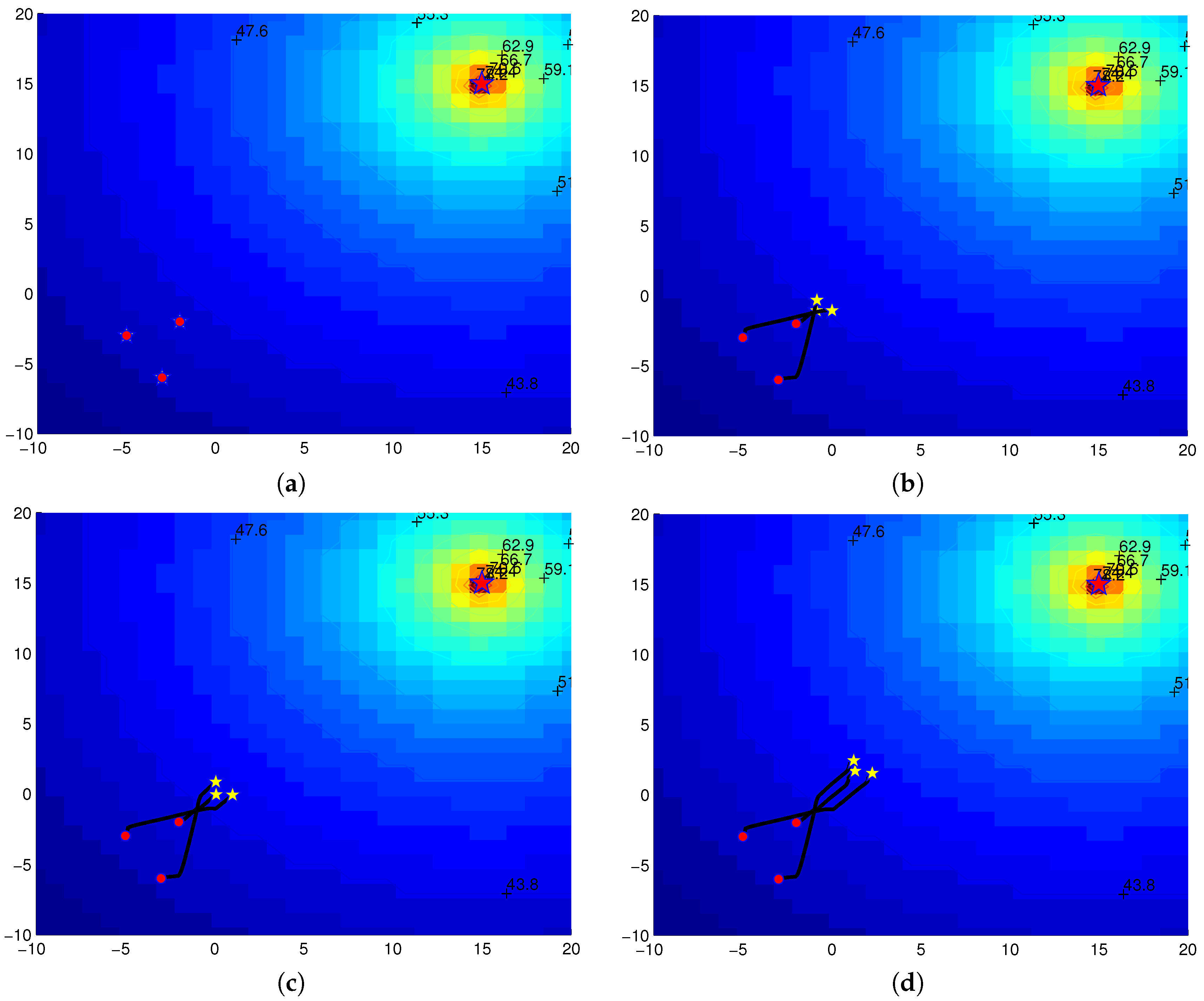
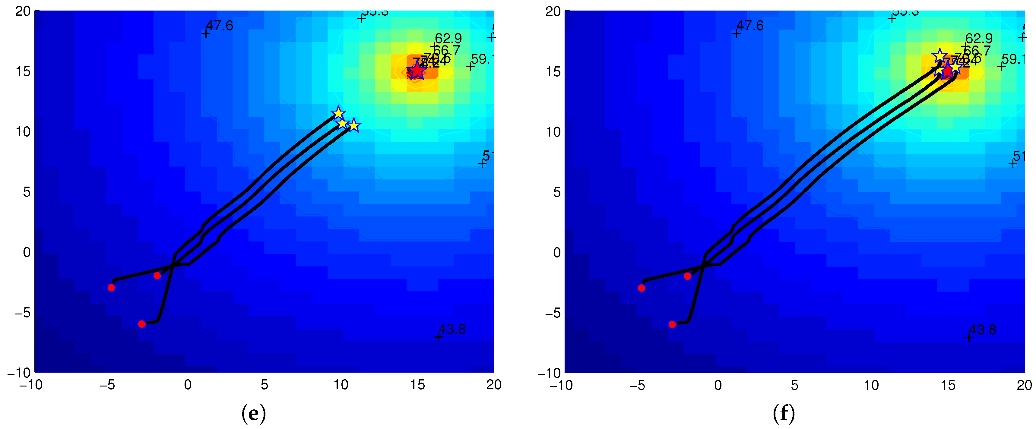
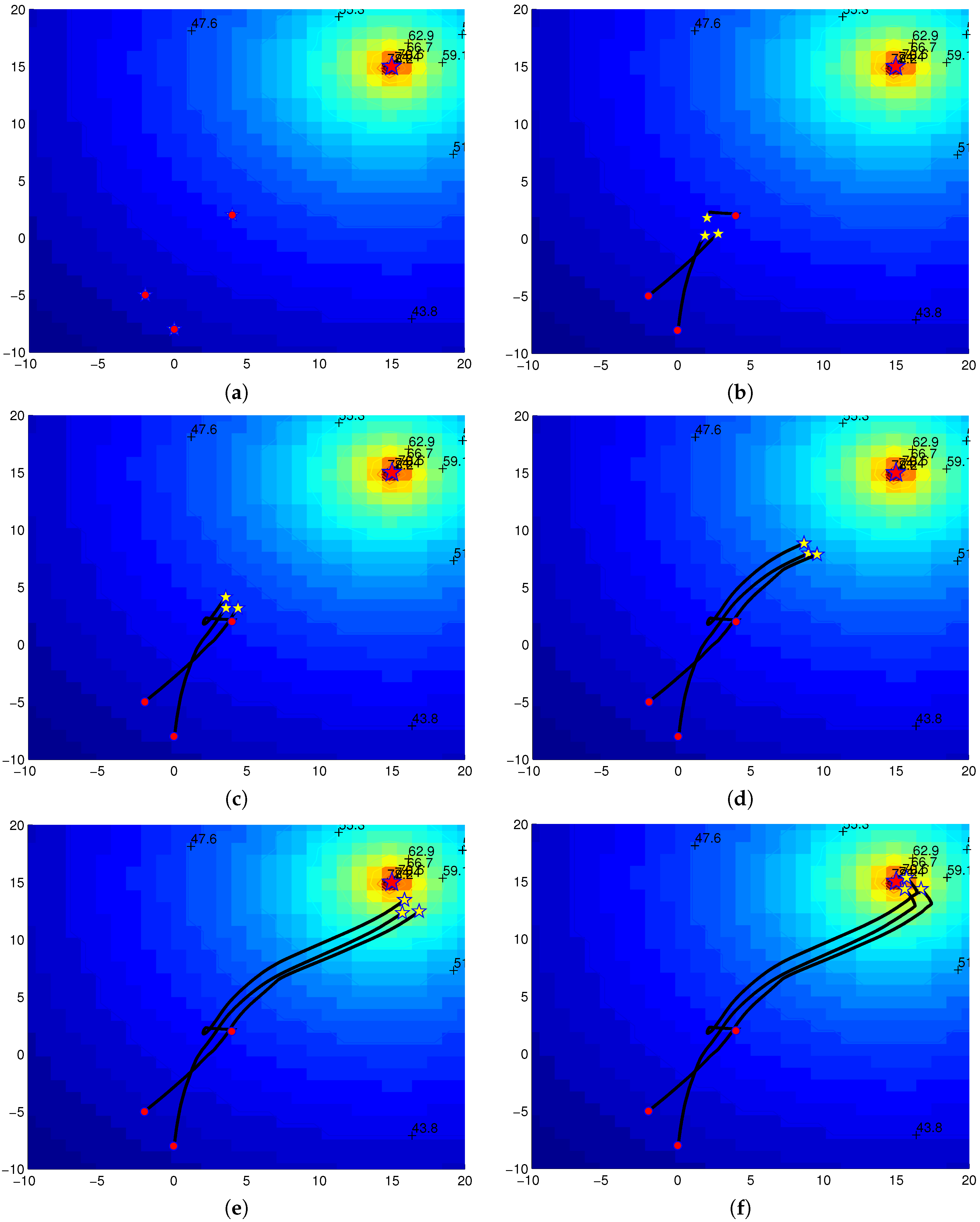
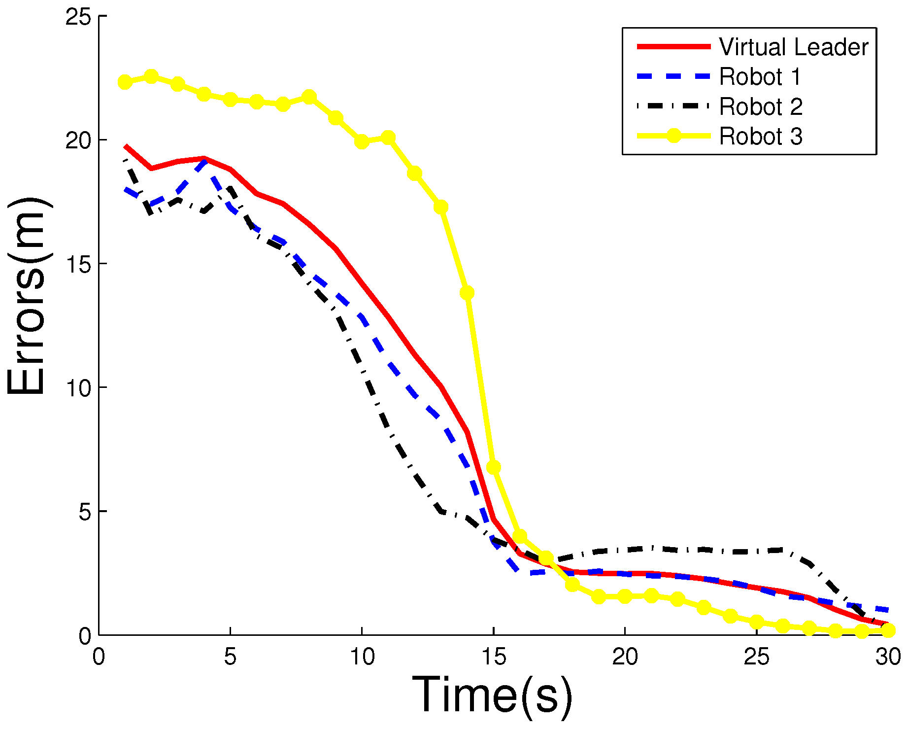
For Case 1, we consider the situation, i.e., the noise variance error $R=5$. Figure 3a–f shows the movement trajectories of robots in one run, from which one can see that the robots can locate the signal source. Moreover, one can see that the red points denote the initial positions; the black lines are the trajectories of three robots; the yellow small stars are the current positions; and the red big star refers to the signal source. Correspondingly, the localization errors $LE$ are illustrated in Figure 4, where one can see that the localization errors $LE$ gradually become small with the movement of robots. Finally, the statistical results for communication frequencies $fre$ and localization errors $LE$ can be found in

Table 3. Mean (standard deviation) results in communication frequency (%) and localization error (m) based on 30 runs for Case 1.

Robots	${\mathit{fre}}_{\mathit{i}}$	${\mathit{LE}}_{\mathit{i}}$
Robot 1	1.81 (0.44)	0.22 (0.16)
Robot 2	8.50 (0.48)	0.25 (0.20)
Robot 3	7.52 (0.53)	0.64 (0.71)

, where 30 runs are conducted, and the corresponding results are small to reflect the effectiveness of the proposed decision-control approach.

4.4. Case 2: The Variance of Noise $R=8$

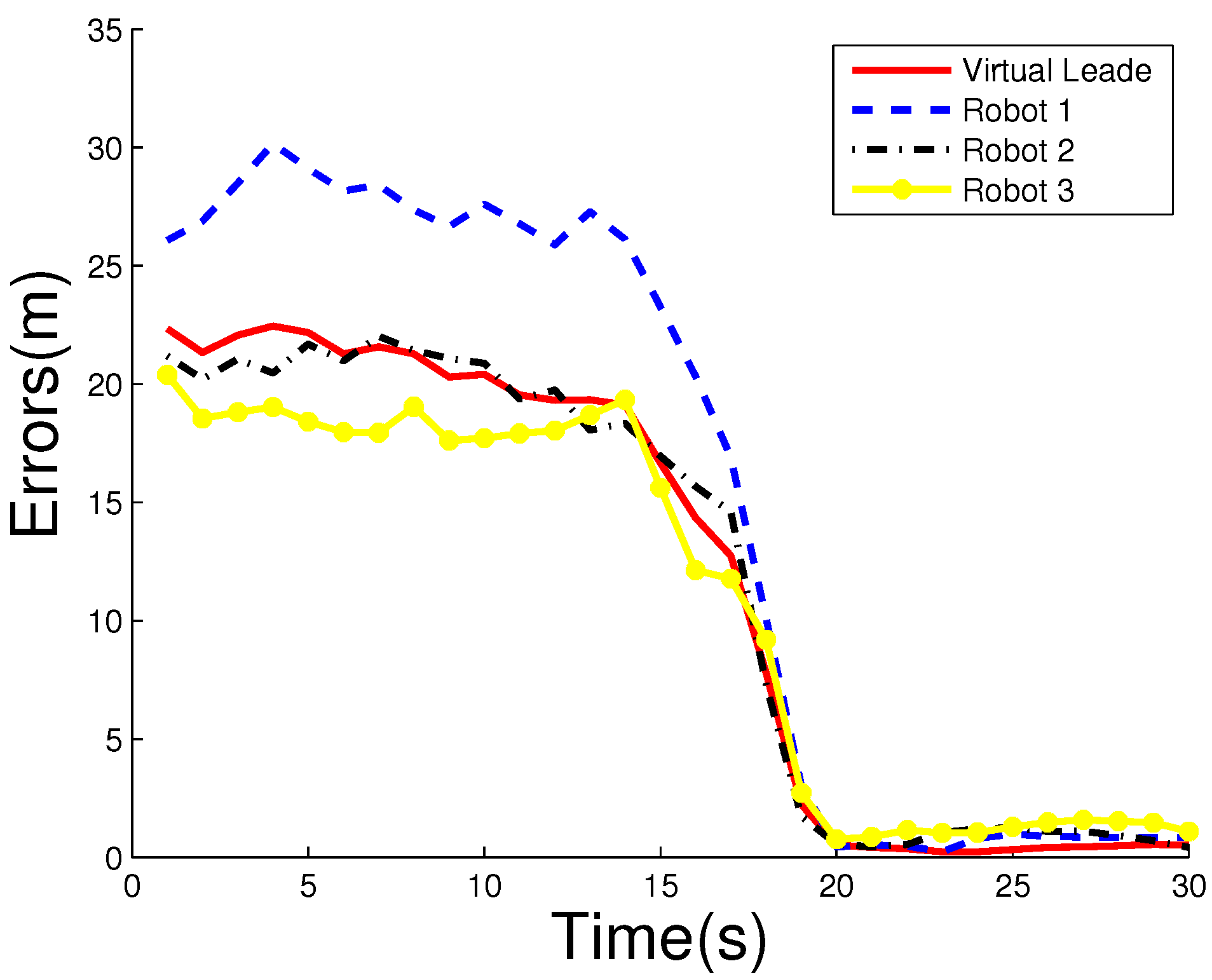
For Case 2, the noise variance error $R=8$ is set in order to evaluate the noise influence on the proposed decision-control approach. The movement trajectories of three robots in one run are illustrated in Figure 5. From this figure, one can see that the three robots can coordinate their behaviors and locate the signal source. Correspondingly, Figure 6 shows the localization errors $LE$, where one can see that the localization errors $LE$ quickly become small such that the signal source is found when the search time approaches 30 s. Finally, we conduct 30 runs and obtain the statistical results for communication frequencies $fr{e}_i$ and localization errors $L{E}_i$, shown in

Table 4. Mean (standard deviation) results in communication frequency (%) and localization error (m) based on 30 runs for Case 2.

Robots	${\mathit{fre}}_{\mathit{i}}$	${\mathit{LE}}_{\mathit{i}}$
Robot 1	1.37 (0.54)	1.07 (0.44)
Robot 2	8.55 (0.50)	1.69 (1.08)
Robot 3	8.07 (0.59)	0.70 (0.71)

. From this table, one can see that the communication frequencies and the localization errors are small, which means that the communication burden is lightened and the proposed decision-control approach can predict the position of signal source under big noise well.

5. Experimental Results

In this section, the proposed decision-control approach is validated by the real experiments where the three Qbot robots are used to locate the signal source.

5.1. Experimental Setup

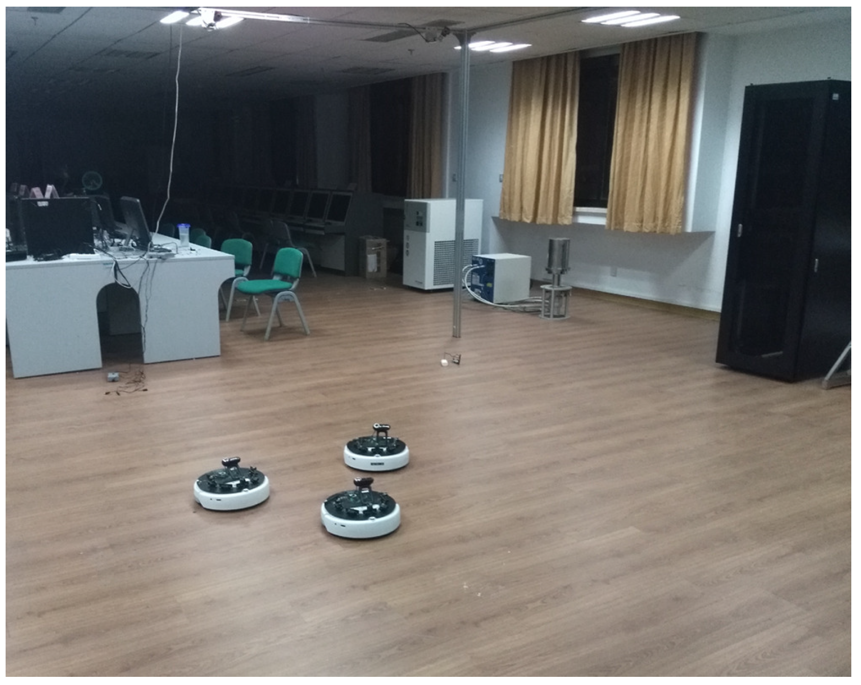
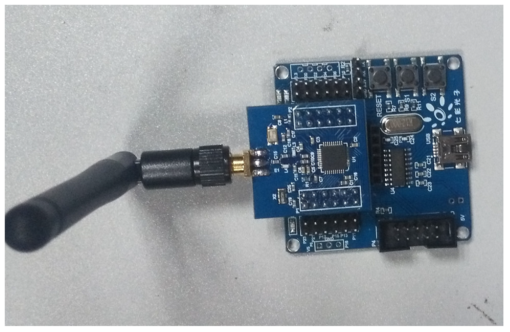
The real experimental environment is shown in Figure 7. Qbot is a differential drive wheeled mobile robot, equipped with two motors, a wireless communication module, an infrared and sonar sensor array and a Logitech Quickcam Pro 9000 USB camera. Moreover, the wireless modules use the ZigBee communication protocol. An electromagnetic module is used as a signal source, shown in Figure 8. At the same time, we employ the OptiTrack system to accurately locate the position of the Qbot. For the robot communication, the Qbots can build a local area network to communicate with each other and establish links with the computer host.

The following function is used to predict the position of the electromagnetic signal source.

$$\begin{array}{c}\hfill f(x,r)=10\times \log \left(0.001\right)-1.96\times \log (\parallel (x-r)\parallel )\end{array}$$

(38)

where r is the particle position for the particle filter. The parameters of Qbot robots are shown in

Table 5. The parameters of Qbot mobile robots.

${\mathit{m}}_{\mathit{i}}$ (kg)	${\mathit{L}}_{\mathit{i}}$ (m)	${\mathit{J}}_{\mathit{i}}$ (kg ${\mathbf{m}}^2$)	b (m)	l (m)	${\mathit{J}}_{\mathit{wheel}}$ (kg ${\mathbf{m}}^2$)
2.92	0.126	0.05	0.03	0.252	0.002

. The parameters of the proposed decision-control approach can be found in Table 2.

5.2. Experimental Results

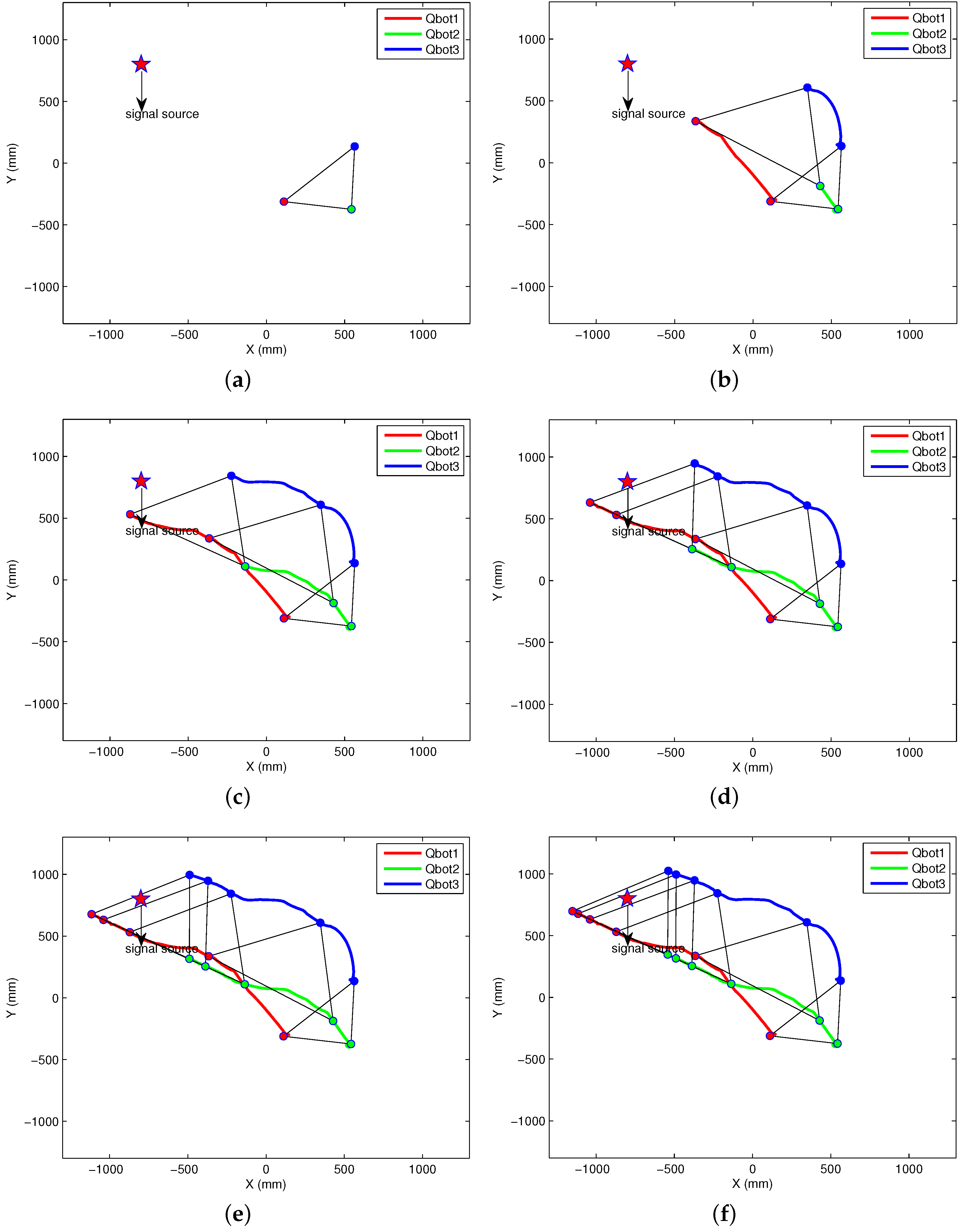
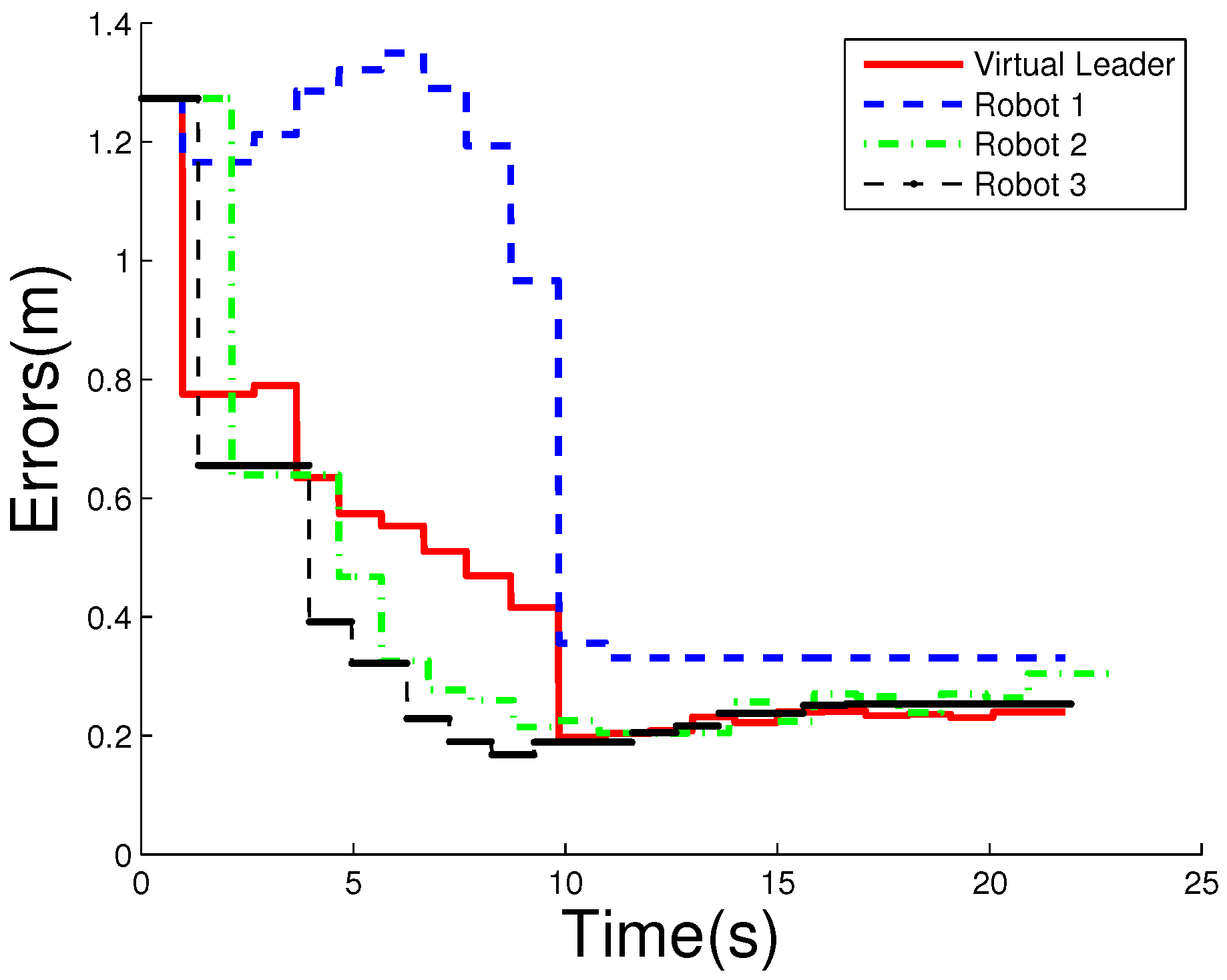
In this subsection, we control three robots to locate an electromagnetic signal source by employing the proposed decision-control approach. The experiments are conducted 30 times. Figure 9 and Figure 10 show movement trajectories and localization errors in one run, respectively. In Figure 9, one can see that three robots can locate the electromagnetic signal source and hold a safe distance from each other, where the different colors denote the different trajectories of robots. Moreover, in Figure 10, the localization errors for three robots are shown, from which one can see that the localization errors are small. Finally, the statistical results for performance metrics are given in

Table 6. Mean (standard deviation) results in communication frequency (%) and localization error (m) based on 30 runs.

Robots	${\mathit{fre}}_{\mathit{i}}$	${\mathit{LE}}_{\mathit{i}}$
Robot 1	6.21 (0.34)	0.30 (0.08)
Robot 2	12.56 (1.05)	0.46 (0.17)
Robot 3	11.64 (1.23)	0.27 (0.07)

, where communication frequencies for three robots are low such that communication burden is well lightened. In addition, the location errors in Table 6 are also small, which implies that the proposed particle filter can predict the position of the electromagnetic signal source well and the proposed decision-control approach can control three robots to keep formation to detect signals well.

6. Conclusions

We have proposed a decision-control approach with the event-triggered communication scheme for the problem of signal source localization. This proposed decision-control approach includes two levels. In the decision level, we have designed a particle filter approach, which is used to estimate the position of signal source. The designed particle filter can guide the movement of robots well under a search environment with big noises. At the control level, we have proposed a cooperative control approach with an event-triggered communication scheme. The proposed event-triggered communication scheme can save communication resources and lighten the communication burden. The simulation and experimental results have illustrated the effectiveness of the proposed decision-control approach.

References

- Lux, R.; Shi, W. Chemotaxis-guided movements in bacteria. Crit. Rev. Oral Biol. Med. 2004, 15, 207–220. [Google Scholar] [CrossRef] [PubMed]
- Lu, Q.; Han, Q.-L.; Zhang, B. Cooperative control of mobile sensor networks for environmental monitoring: An event-triggered finite-time control scheme. IEEE Trans. Cybern. 2017, 47, 4134–4147. [Google Scholar] [CrossRef] [PubMed]
- Lu, Q.; Liu, S.; Xie, X.; Wang, J. Decision-making and finite-time motion control for a group of robots. IEEE Trans. Cybern. 2013, 43, 738–750. [Google Scholar] [PubMed]
- Zhang, X.; Fang, Y.; Sun, N. Visual servoing of mobile robots for posture stabilization: From theory to experiments. Int. J. Robust Nonlinear Control 2015, 25, 1–15. [Google Scholar] [CrossRef]
- Zhang, X.; Fang, Y.; Liu, X. Motion-estimation-based visual servoing of nonholonomic mobile robots. IEEE Trans. Robot. 2011, 27, 1167–1175. [Google Scholar] [CrossRef]
- Wang, Y.-L.; Han, Q.-L. Network-based modeling and dynamic output feedback control for unmanned marine vehicles. Automatica 2018, 91, 43–53. [Google Scholar] [CrossRef]
- Wang, Y.-L.; Han, Q.-L.; Fei, M.; Peng, C. Network-based T-S fuzzy dynamic positioning controller design for unmanned marine vehicles. IEEE Trans. Cybern. 2018. [Google Scholar] [CrossRef]
- Sukhatme, G.S.; Dhariwal, A.; Zhang, B. Design and development of a wireless robotic networked aquatic microbial observing system. Environ. Eng. Sci. 2007, 24, 205–215. [Google Scholar] [CrossRef]
- Kumar, V.; Rus, D.; Singh, S. Robot and sensor networks for first responders. IEEE Pervasive Comput. 2004, 3, 24–33. [Google Scholar] [CrossRef] [Green Version]
- Ferreira, N.L.; Couceiro, M.S.; Araujo, A. Multi-sensor fusion and classification with mobile robots for situation awareness in urban search and rescue using ROS. In Proceedings of the 2013 IEEE International Symposium on Safety, Security, and Rescue Robotics, Linkoping, Sweden, 21–26 October 2013; pp. 1–6. [Google Scholar]
- Azuma, S.I.; Sakar, M.S.; Pappas, G.J. Stochastic source seeking by mobile robots. IEEE Trans. Autom. Control 2012, 57, 2308–2321. [Google Scholar] [CrossRef] [Green Version]
- Zhang, C.; Arnold, D.; Ghods, N. Source seeking with non-holonomic unicycle without position measurement and with tuning of forward velocity. Syst. Control Lett. 2007, 56, 245–252. [Google Scholar] [CrossRef]
- Liu, S.J.; Krstic, M. Stochastic source seeking for nonholonomic unicycle. Automatica 2012, 46, 1443–1453. [Google Scholar] [CrossRef]
- Song, D.; Kim, C.Y.; Yi, J. Simultaneous localization of multiple unknown and transient radio sources using a mobile robot. IEEE Trans. Robot. 2012, 28, 668–680. [Google Scholar] [CrossRef]
- Bachmayer, R.; Leonard, N.E. Vehicle networks for gradient descent in a sampled environment. In Proceedings of the 41st IEEE Conference on Decision and Control, Las Vegas, NV, USA, 10–13 December 2002; pp. 112–117. [Google Scholar]
- Moore, B.J.; Canudas-De-Wit, C. Source seeking via collaborative measurements by a circular formation of agents. In Proceedings of the 2010 American Control Conference, Baltimore, MD, USA, 30 June–2 July 2010; pp. 1292–1302. [Google Scholar]
- Ogren, P.; Fiorelli, E.; Leonard, N.E. Cooperative control of mobile sensor networks: Adaptive gradient climbing in a distributed environment. IEEE Trans. Autom. Control 2004, 49, 1292–1302. [Google Scholar] [CrossRef]
- Atanasov, N.A.; Ny, J.L.; Pappas, G.J. Distributed algorithms for stochastic source seeking with mobile robot networks. J. Dyn. Syst. Meas. Control 2014, 137, 031004/1–031004/9. [Google Scholar] [CrossRef]
- Li, S.; Kong, R.; Guo, Y. Cooperative distributed source seeking by multiple robots: Algorithms and experiments. IEEE/ASME Trans. Mechatron. 2014, 19, 1810–1820. [Google Scholar] [CrossRef]
- Zhang, X.; Fang, Y.; Li, B.; Wang, J. Visual servoing of nonholonomic mobile robots with uncalibrated camera-to-robot parameters. IEEE Trans. Ind. Electron. 2017, 64, 390–400. [Google Scholar] [CrossRef]
- Zhang, X.; Wang, R.; Fang, Y.; Li, B.; Ma, B. Acceleration-level pseudo-dynamic visual servoing of mobile robots with backstepping and dynamic surface control. IEEE Trans. Syst. Man Cybern. Syst. 2017. [Google Scholar] [CrossRef]
- Oyekan, J.; Gu, D.; Hu, H. Hazardous substance source seeking in a diffusion based noisy environment. In Proceedings of the 2012 International Conference on Mechatronics and Automation (ICMA), Chengdu, China, 5–8 August 2012; pp. 708–713. [Google Scholar]
- Ge, X.; Han, Q.-L.; Yang, F. Event-based set-membership leader-following consensus of networked multi-agent systems subject to limited communication resources and unknown-but-bounded noise. IEEE Trans. Ind. Electron. 2017, 64, 5045–5054. [Google Scholar] [CrossRef]
- Cao, Y.; Yu, W.; Ren, W.; Chen, G. An overview of recent progress in the study of distributed multi-agent coordination. IEEE Trans. Ind. Inform. 2013, 9, 427–438. [Google Scholar] [CrossRef]
- Jiang, Y.; Zhang, H.; Chen, J. Sign-consensus of linear multi-agent systems over signed directed graphs. IEEE Trans. Ind. Electron. 2017, 64, 5075–5083. [Google Scholar] [CrossRef]
- Valcher, M.E.; Zorzan, I. On the consensus of homogeneous multi-agent systems with positivity constraints. IEEE Trans. Autom. Control 2017, 62, 5096–5110. [Google Scholar] [CrossRef]
- Garca-Magario, I.; Gutirrez, C.; Fuentes-Fernndez, R. The INGENIAS development kit: A practical application for crisis-management. In Proceedings of the 10th International Work-Conference on Artificial Neural Networks (IWANN 2009), Salamanca, Spain, 10–12 June 2009; Volume 5517, pp. 537–544. [Google Scholar]
- Garca-Magario, I.; Gutirrez, C. Agent-oriented modeling and development of a system for crisis management. Expert Syst. Appl. 2013, 40, 6580–6592. [Google Scholar] [CrossRef]
- Zou, R.; Kalivarapu, V.; Winer, E.; Oliver, J. Particle swarm optimization-based source seeking. IEEE Trans. Autom. Sci. Eng. 2015, 12, 865–875. [Google Scholar] [CrossRef]
- Li, H.; Liao, X.; Huang, T. Event-triggering sampling based leader-following consensus in second-order multi-agent systems. IEEE Trans. Autom. Control 2015, 60, 1998–2003. [Google Scholar] [CrossRef]
- Xie, D.; Xu, S.; Zhang, B. Consensus for multi-agent systems with distributed adaptive control and an event-triggered communication strategy. IET Control Theory Appl. 2016, 10, 1547–1555. [Google Scholar] [CrossRef]
- Zhu, W.; Jiang, Z.P. Event-based leader-following consensus of multi-agent systems with input time delay. IEEE Trans. Autom. Control 2015, 60, 1362–1367. [Google Scholar] [CrossRef]
- Dimarogonas, D.V.; Johansson, K.H. Event-triggered control for multi-agent systems. In Proceedings of the 48th Decision and Control, 2009 Held Jointly with the 2009 28th Chinese Control Conference, Shanghai, China, 15–18 December 2009; pp. 7131–7136. [Google Scholar]
- Dimarogonas, D.V.; Frazzoli, E.; Johansson, K.H. Distributed event-triggered control for multi-agent systems. IEEE Trans. Autom. Control 2012, 57, 1291–1297. [Google Scholar] [CrossRef]
- Fan, Y.; Feng, G.; Wang, Y. Distributed event-triggered control of multi-agent systems with combinational measurements. Automatica 2013, 49, 671–675. [Google Scholar] [CrossRef]
- Zhang, H.; Feng, G.; Yan, H. Observer-Based Output Feedback Event-Triggered Control for Consensus of Multi-Agent Systems. IEEE Trans. Ind. Electron. 2014, 61, 4885–4894. [Google Scholar] [CrossRef]
- Lawton, J.R.T.; Beard, R.W.; Young, B.J. A decentralized approach to formation maneuvers. IEEE Trans. Robot. Autom. 2003, 19, 933–941. [Google Scholar] [CrossRef] [Green Version]
Figure 1.
Search environment where the red point denotes the robot, and the red star is the signal source. The colors of the background represent the signal strength and are also labeled by the numbers.
Figure 2.
The Qbot robot.
Figure 3.
Movement trajectories of three robots for Case 1 where the red points denote the initial positions, the black lines are the trajectories of three robots, the yellow small stars are the current positions and the red big star refers to the signal source. The colors of the background represent the signal strength and are also labeled by the numbers. The signal strength increases with the decrease of the distance from the source. (a) t = 0 s; (b) t = 5 s; (c) t = 10 s; (d) t = 15 s; (e) t = 20 s; (f) t = 30 s.
Figure 4.
The curves for the localization errors for Case 1.
Figure 5.
Movement trajectories of three robots for Case 2 where the red points denote the initial positions, the black lines are the trajectories of three robots, the yellow small stars are the current positions and the red big star refers to the signal source. The colors of the background represent the signal strength and are also labeled by the numbers. The signal strength increases with the decrease of the distance from the source. (a) t = 0 s; (b) t = 5 s; (c) t = 10 s; (d) t = 15 s; (e) t = 20 s; (f) t = 30 s.
Figure 6.
The curves for the localization errors for Case 2.
Figure 7.
Experimental environment.
Figure 8.
An electromagnetic signal source.
Figure 9.
Movement trajectories of three robots where the red, blue and green lines denote the trajectories of three robots. (a) t = 0 s; (b) t = 4 s; (c) t = 8 s; (d) t = 12 s; (e) t = 16 s; (f) t = 20 s.
Figure 10.
The curves for the localization errors.