1. Introduction
Since the first laser developments, Holographic Data Storage Systems (HDSS) have been a promising and appealing technology for true 3D storage of information and associative memory retrieval [
1,
2]. There are some scientific and technological challenges to fulfill when a HDSS is developed [
3,
4].
Our group evaluated the introduction of some novelties in the HDSS. One of these is the introduction of a parallel-aligned liquid crystal on silicon (PA-LCoS) microdisplay [
5]. The PA-LCoS acts as data pager, and we designed some modulation schemes for it [
6]. In this paper, we present a characterization method that allows us to evaluate the limitations introduced by different elements in our optical system.
In previous works, we developed a characterization method for PA-LCoS, enabling to characterize the flicker effects produced because of the digital addressing technology, and also to characterize the retardance introduced [
7]. In the literature, other degradation phenomena have also been detected and analyzed related not only with modern PA-LCoS microdisplays but also with previous liquid crystal displays (LCD). An important one is the anamorphic and frequency dependent effect [
8,
9,
10,
11] that causes a reduction in the performance depending on the spatial frequency and on the orientation of the image displayed. In this sense, the anamorphic frequency dependent effect is exhibited by liquid crystal displays (LCDs) [
8,
9,
11] and by modern LCoS devices, both digital [
10] and analogically [
11] driven. In LCDs, it was demonstrated [
9] that the anamorphic phenomenon was directly related with the electronics driving the device. In general, the electrical signal corresponding to an image addressed to the display is produced by multiplexing the rows composing the image, where each row contains the voltage value to be applied to each of the pixels in the row. As a result, the horizontal (or pixel) frequency in the electrical signal is much larger than the vertical (or row) frequency. The limited bandwidth of the electronics driver will then produce a low-pass filtering for the horizontal frequency components in the image, especially if the image contains fast variations along the horizontal. This low-pass filtering of the electrical signal is then reflected on the reduction of the phase modulation range available when displaying phase-only diffractive optical elements [
8]. The anamorphic and frequency dependent phenomenon has also been reported when using the LCD in the amplitude-only regime [
3,
12,
13,
14,
15]. The authors were interested on the characterization of the modulation transfer function (MTF) of the LCD for its application in optical processing [
12,
13,
14]. In [
3] (p. 247) and [
15], the LCD is applied in holographic data storage, which is also the focus of the present paper.
Besides the effects produced by the limited electronics bandwidth already described, interpixel effects in the LC layer may also cause a reduction in the spatial frequency bandwidth. These interpixel effects are the fringing-field (i.e., appearance of tangential components in the applied electric field) and vicinity LC adherence effects that appear as a result of the competition between the tangential components of the applied field and the intermolecular forces within the liquid crystals (i.e., avoiding abrupt changes in the orientation) [
16,
17,
18,
19,
20,
21,
22]. These interpixel effects are becoming more and more important in modern LCoS devices as the pixel size is becoming increasingly small, even smaller than 4 µm [
22], thus decreasing the ratio between the pixel size and the LC layer thickness (i.e., the cell gap). We also note that vicinity LC adherence effects exhibit an anamorphic behavior, as described in numerical simulations by Wang et al. [
18], depending on whether the applied electric voltage gradient is along the LC director at the alignment layers or perpendicular.
Our first goal in this paper is to identify if the anamorphic and frequency dependent phenomenon affects our particular application, which in the present case is the application of PA-LCoS microdisplays to holographic data storage. We also need to test other limitations such as the maximum resolution of the optical system, aberrations, etc. We want to know the origin of these limitations to change the setup to improve the performance and to know our practical data storage capacity.
In this paper, we focus in the complete optical system. Thus, we evaluate the limitations due to the lenses, the ones added by the PA-LCoS microdisplay, and the illumination. All this work is necessary prior to the introduction of the holographic material, which adds additional degradation effects. The methodology that we propose is not only able to provide a global characterization of the HDSS, but also to perform a local and quantitative characterization across the aperture of the system. This local characterization is very useful to evaluate nonuniformity of the illumination, spatial variant response of the LCoS device, and misalignments of the elements in the system.
As we are managing a binary data storage system, to study the influence of the different elements, we measured the Bit Error Rate (BER) or the Quality factor (Q-factor), figures of merit defined for digital data transmission systems. We analyzed the errors retrieved in the reconstructed image by means of a CCD camera.
We show how the introduction of the material affects the performance. We used Polyvinyl Alcohol Acrylamide (PVA/AA) that was produced, characterized and modeled by our group [
23]. These preliminary results show us how to improve the process of producing and depositing PVA/AA for holographic data storage applications.
2. Experimental Setup
In our HDSS, we used a convergent processor architecture for the object beam. This setup is also known as VanderLugt correlator [
24]. This alternative provided us some flexibility. It allowed a wider freedom when selecting lenses to be used, because it is not necessary that the focal lengths match, as is the case in the classical 4-f system. Furthermore, the areal density on the recording material can be varied without the need to change the lenses, as explained in [
25].
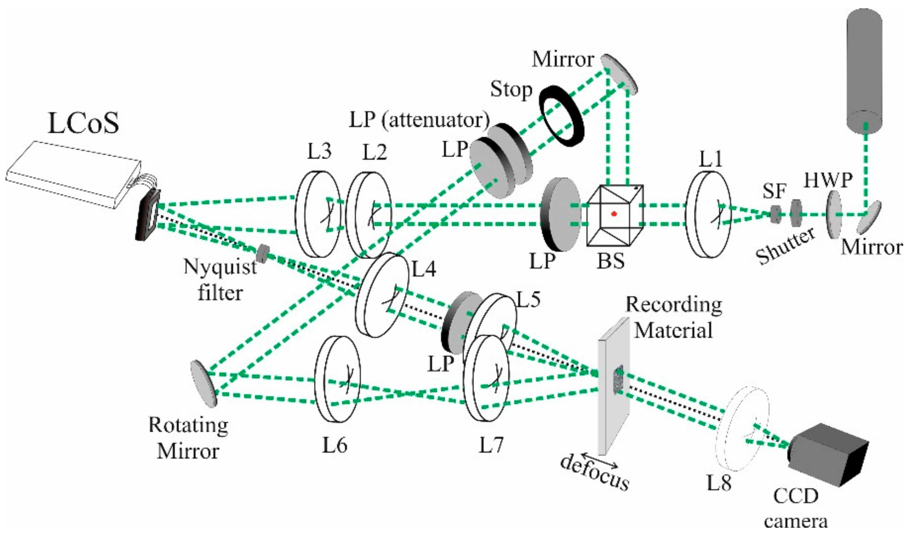
In
Figure 1, we show the complete experimental setup. The object beam follows the path formed by lenses L2 to L5. Along the same optical axis, we have lens L8 to form the image of the data page onto the CCD camera plane. Path formed by lenses L6 and L7 is the reference beam. In our discussion about limitations, we only refer to the object beam combined with lens L8.
In the object beam, we introduced the data page by means of the PA-LCoS. The display was placed after the L3 lens. We used a divergent lens L2, so that the combination of L2 and L3 enables to modify the convergence angle of the beam onto the LCoS. The beam impinges onto the PA-LCoS while it is converging. The Fourier transform forms at the convergence plane, where we placed a Nyquist filter to control the Fourier Transform orders that we store. Lenses L4 and L5 form a relay system to image the Nyquist filter plane, which contains our information, onto the recording plane. In the present work, we did not use the filtering option by the Nyquist filter, since our focus was the study of the anamorphic and optical limitations of our system.
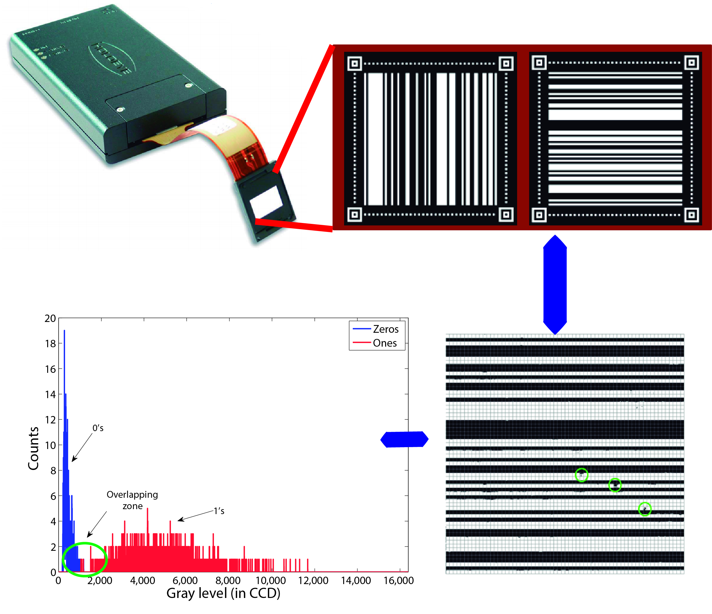
The PA-LCoS used in this work is a commercially available PA-LCoS microdisplay, model PLUTO distributed by the company HOLOEYE. It is filled with a nematic liquid crystal, with 1920 × 1080 pixels and 0.7'' diagonal. The fill factor is 87% and its pixel pitch is 8.0 μm. It is important to remark the pixel pitch, because it defines the information bit size for different resolutions. The incident angle to separate impinging and reflecting object beam is 11.5°, and it is fixed during all the experiment.
We used different numbers of pixels in the PA-LCoS to form a bit of information. These bit sizes were: 8 × 8, 4 × 4, 3 × 3, and 2 × 2 pixels. This means that, for every bit of information, we used, respectively, 64, 16, 9 and 4 pixels in the PLUTO device. Thus, they have, respectively, a 64 μm, 32 μm, 24 μm, and 16 μm length in each side for the square that forms the information bit. In this work, we aggregated the bits in the shape of linear stripes, arranged in a vertical or horizontal orientation, because we wanted to test if the reduction in the performance of the HDSS system is related to an anamorphic effect in the PA-LCoS. In this context, the bit size defines the minimum stripe width. In the data analysis, for statistical reasons, we considered individual bits of information, instead of individual stripes, to calculate the Bit Error Rate: in this way, we ensured that we have enough information to statistically analyze the image. We addressed LCoS data pages with 512 × 512 pixels. If we would consider stripes as a block of information, we would only have 64 information blocks for 8 × 8 pix. size, 128 for 4 × 4, etc. Considering individual bits, we have 4096 bits of information for 8 × 8 pix. size, 16,384 for 4 × 4, etc.
To retrieve information, we used a CCD camera. We used the PCO.1600 model from PCO.imaging company. This is a high dynamic 14-bit cooled CCD camera with a resolution of 1600 × 1200 pixels, and a pixel size of 7.4 × 7.4 μm2. The magnification of the PA-LCoS plane onto the camera plane is about a factor of two. Therefore, there is no limitation from the CCD camera since the image built on the CCD plane is oversampled.
3. Characterization Method
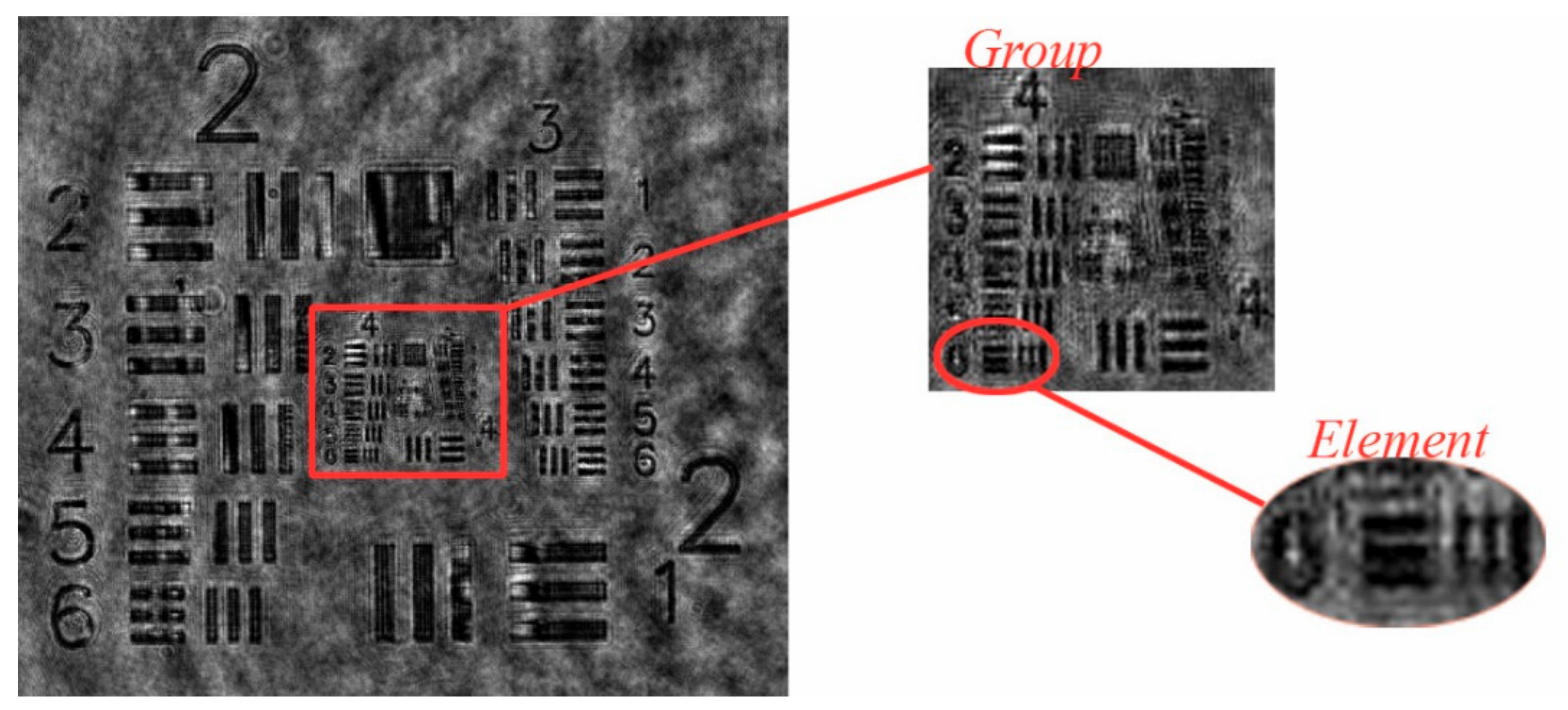
When analyzing the data storage system, we find various sources of limitations. The initial one is produced by the aperture of the lenses. For that reason, we have to test the resolution capability of our setup by using a standard 1951 USAF test target. So, the first step for characterizing the optical system is to obtain the resolving power of the complete optical system composed of lenses L4, L5 and L8. To do that, we relay the image from the PA-LCoS plane onto the CCD camera but we place a negative 1951 USAF resolution test chart instead of our PA-LCoS device, and we capture the reflected image with the help of the CCD camera. Reference beam is blocked and no recording material is introduced.
In
Figure 2, we show the retrieved image of the 1951 USAF resolution test target. From this image, we conclude that our limit is Group 4 element 6 for both horizontal and vertical orientation, which corresponds to a resolution of 28.50 lp/mm or equivalently 35.09 μm per line pair. This a line width of 17.54 μm, which, translated into pixels in our PA-LCoS, means that a stripe width of two pixels (8 + 8 μm) cannot be resolved.
Once we calculated our optical system resolution limit, we introduced the PA-LCoS instead of the USAF resolution test target. We evaluated whether there were additional limitations related with the well-known anamorphic effects presented by this kind of microdisplays [
10,
11,
22]. To do that, in our optical system, we prepared some test patterns with different resolutions and with two orientations, vertical and horizontal.
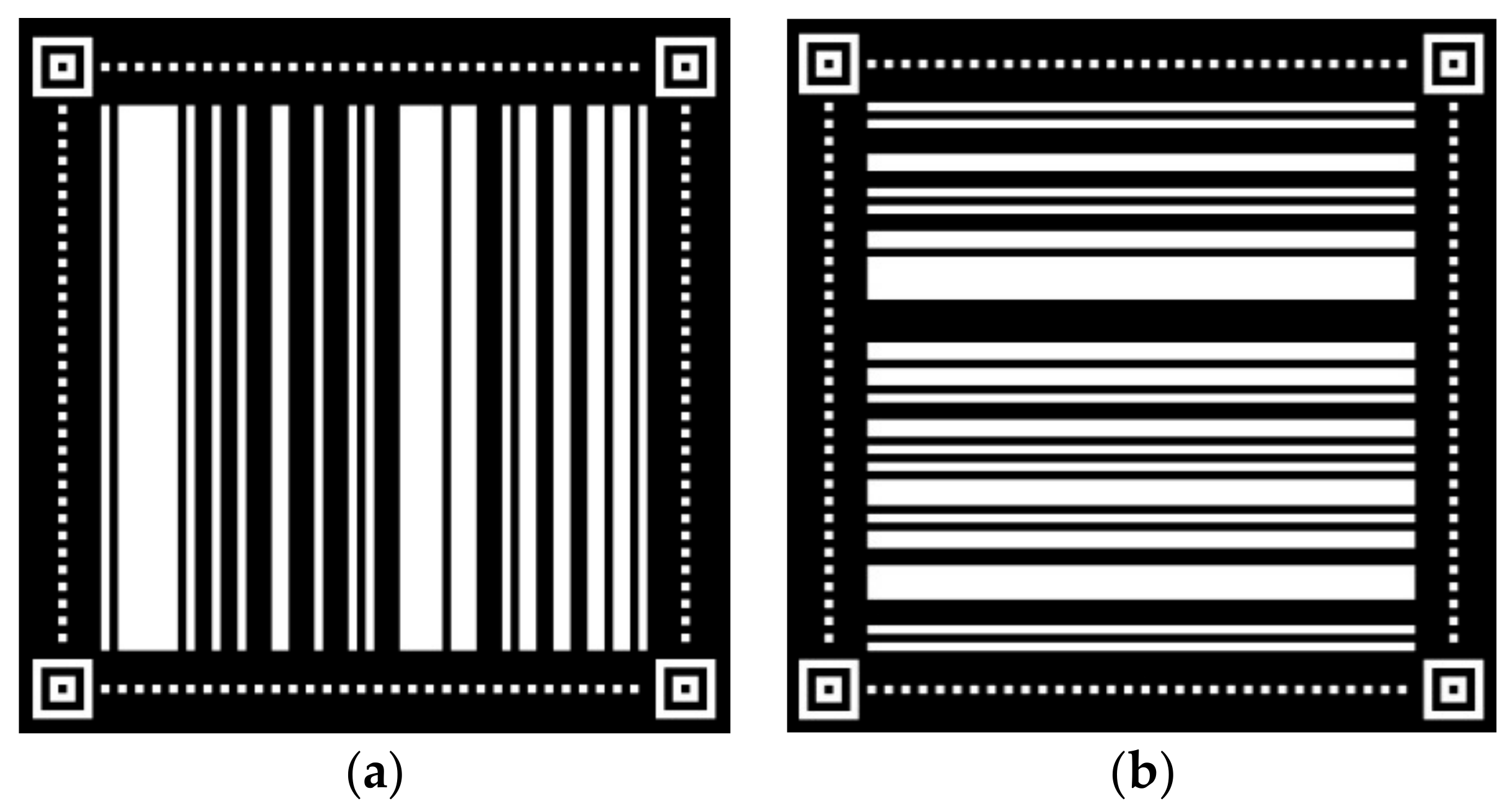
The images have the aspect presented in
Figure 3, where we show the pattern that corresponds with a bit size of 8 × 8 pixels in the PA-LCoS. We alternated between black and white stripes of a selected width. The position and width of the stripeswere generated in a random way to avoid periodic diffractive effects. We added fiducial marks for centering and rotation, and to detect the position of the information bits. These marks also enabled evaluating the quality of the image or distortion during the capture. The width of the lines composing the fiducial marks was always 8 pixels, which was our reference to evaluate the resolution used in the data page in the case we do not know it.
We configured our setup for binary intensity modulation (BIM) [
6]. To do that, we uploaded to the PA-LCoS an electrical configuration that offers a 180° retardance range, with a good linearity, and permitted obtaining the maximum contrast and less flicker, as we analyzed in [
26]. The maximum contrast would be produced when the polarizers in the object beam are crossed with respect to each other and they form a 45° angle with respect to the alignment direction of the LC director in the PA-LCoS display.
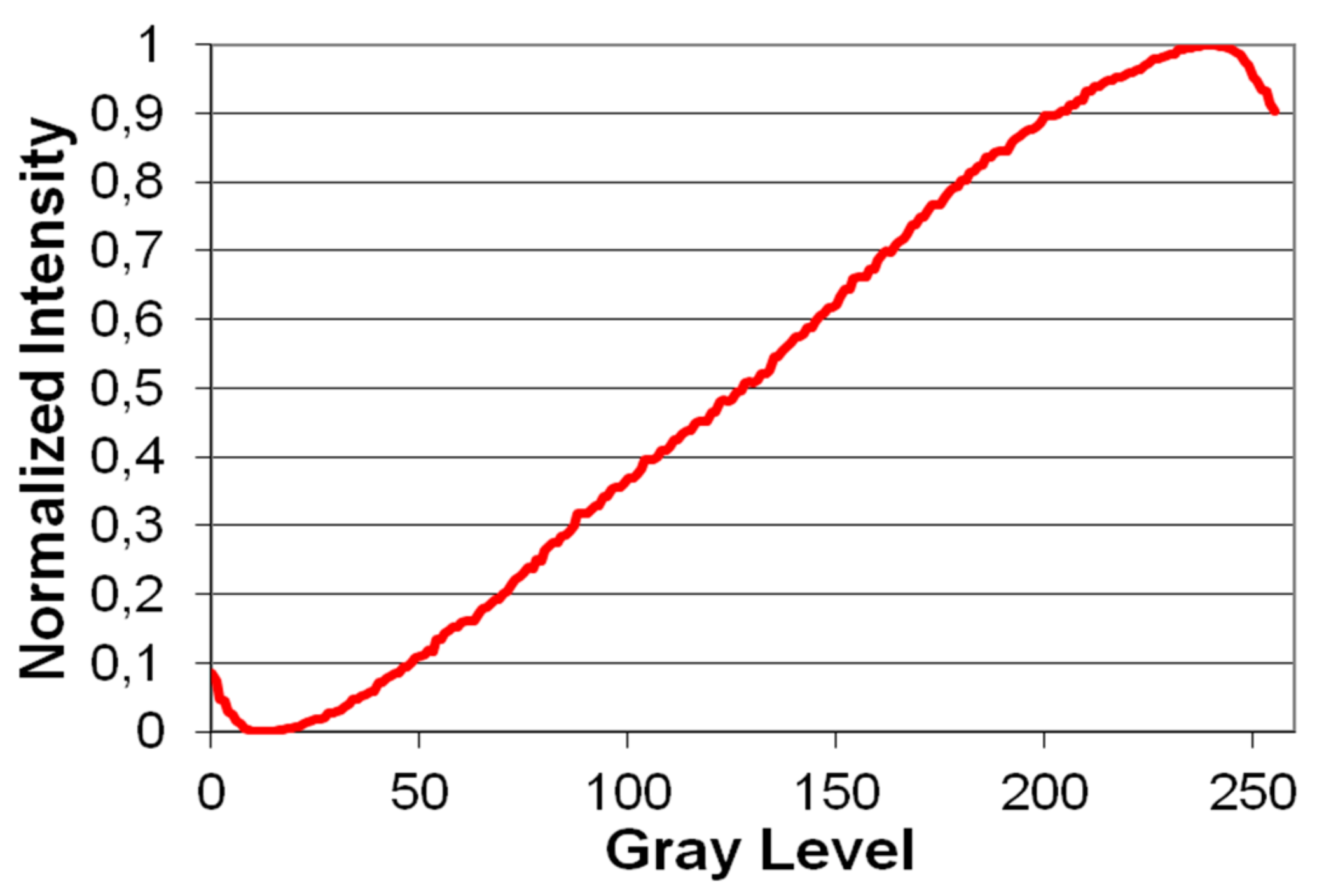
In
Figure 4, we show the calibration measurements done for the PA-LCoS. These calibration measurements were obtained with the configuration described above, and the 11.5° incident angle commented in the setup description. As we used BIM, we only used two values of gray level. These values have to offer the maximum contrast. In
Figure 4, we selected gray level 14 as black level (lowest intensity) and gray level 248 as white level (highest intensity).
To analyze the errors introduced by the optical system, we illuminated the PA-LCoS (see
Figure 1) and, through lenses L4, L5 and L8, we produced the image of the data page onto the CCD camera [
25]. The image data obtained was then digitally analyzed [
6]. We note that positions for lenses L4, L5 and L8 are the same as in the previous characterization step with the USAF resolution test target and there is no recording material in the system.
After capturing the image with the CCD camera and before processing the image to convert it into a binary image, we extracted the region of the image that contains the data, i.e., the stripes region. To detect this region, we used fiducial marks. These marks allowed calculating the scale factor introduced, the rotation, and the possible distortion effects produced by the optical setup. The rotation can be corrected by software to prepare the image to extract the data.
We applied some processing operations in the captured image to retrieve the information stored. These processing operations were also applied when we proceeded, afterwards, with the characterization of the complete system in conjunction with recording material. Since we used a binary image, we selected the best threshold value to distinguish between the 0 level and the 1 level. For that reason, we thresholded the image by selecting the appropriate value of the gray level to separate the 0s from the 1s. We analyzed various values to select the level that minimizes the detected errors, and for every gray level we calculate the BER. The CCD has a bit depth of 14 bits, which means that we have values from 0 to 16384.
One possibility is to calculate the BER by counting directly the falsely detected bits in the image. To this goal, we first applied a thresholding. In this way, we obtained a binary image. Then, we compared the bits in the binary image obtained with the bits in the original data set displayed in the PA-LCoS, which must to be done for every threshold gray level considered. In the thresholded image, the bit is composed of a block of CCD pixels. We considered the value of the central CCD pixel as the value for the bit. By counting the number of errors, we could calculate the BER. This BER was calculated by dividing the number of errors by the total number of bits. The total number of bits depends on the resolution selected, which means that for a 8 × 8 bit size we have 64 × 64 (4096) bits of information, 128 × 128 (16,384) bits for 4 × 4 bit size, 170 × 170 (28,900) bits for 3 × 3 bit size and 256 × 256 (65,536) bits for a 2 × 2 bit size.
This form of calculating the BER can be useful as a first approximation but it depends too much on the specific image captured. Therefore, it is better to calculate the Q-factor, which offers an estimation measure for the quality of the signal-to-noise ratio. This Q-factor is calculated from the probability distribution of 1s and 0s from the unprocessed images. As long as we can infer the positions of the 1s and 0s, we can obtain a histogram of 1s and 0s and calculate this Q-factor that it is typically used in digital systems in fiber optics communications [
27,
28,
29]. Q-factor is given by,
where
μ1 and
μ0 are the mean value in the histograms produced for the gray level distribution of ON and OFF bits, respectively, and
σ1 and
σ0 are the corresponding standard deviations. If the histograms are approximated as Gaussian distributions, the relation between BER and Q-factor is given by,
where
erf is the error function [
27,
28,
29], which is tabulated in various mathematical handbooks [
30,
31]. These values show the capacity of the optical system to recover the digital information introduced. We needed a raw BER in the range of 10
−3 to assure a complete information recovery after introducing error correction codes.
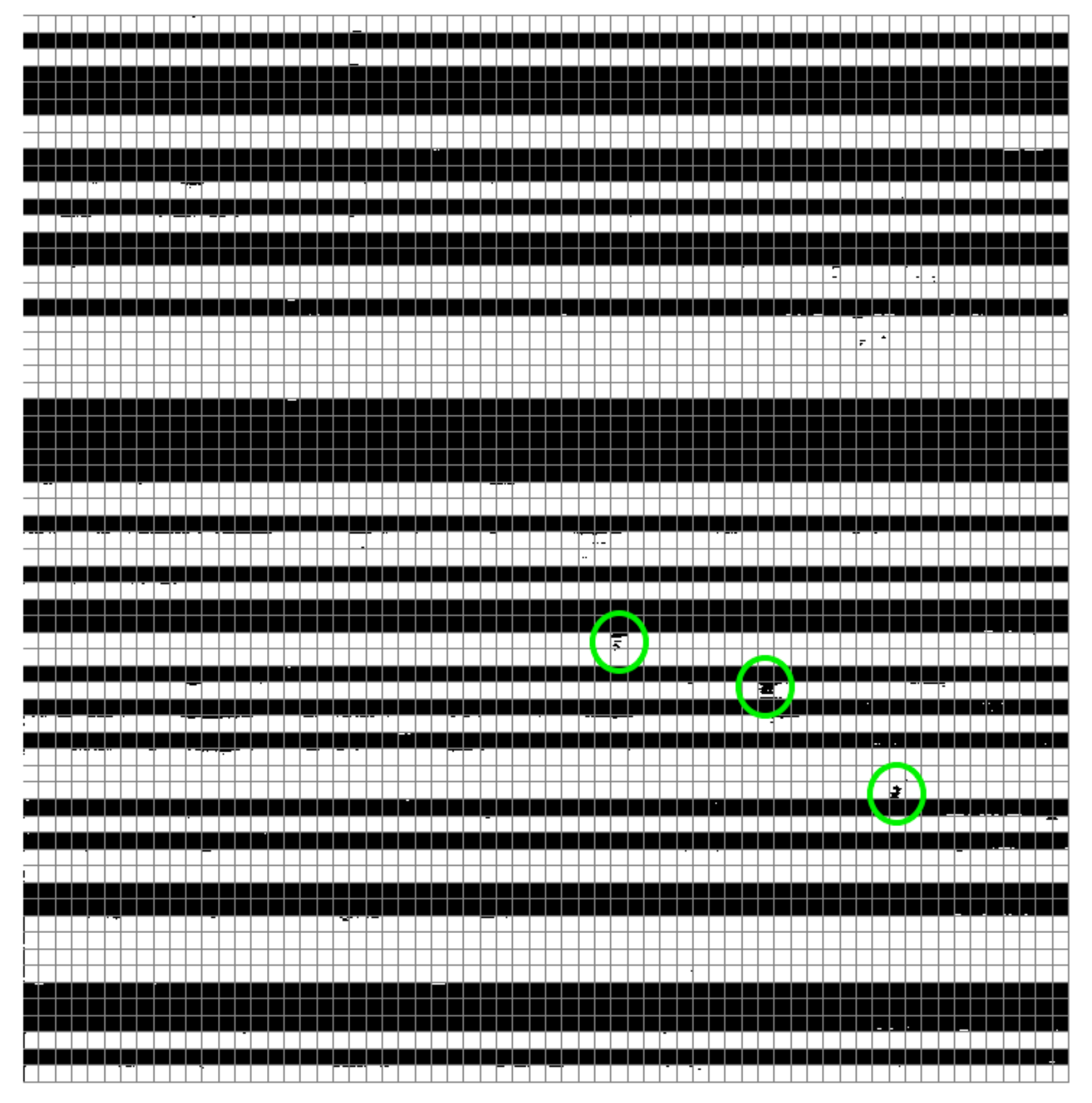
In
Figure 5, we show a thresholded image captured for a data page with a pixel size of 8 × 8 (8 × 8 pixels in the PA-LCoS for each bit of information).
Figure 5 also shows the division of the image in bits, given by the overlain grid pattern. We present this image to illustrate that, even though the images proposed in the study only have information in a specific direction (horizontal or vertical), to allow a statistical analysis, we analyzed the image at a bit level.
Figure 5 represents the best thresholded image detected for an 8 × 8 data page; to make the bits more visible, we have used the biggest bit size. These 8 × 8 pixels per bit are referred to the image displayed in the PA-LCoS. The image shown in
Figure 5 is the image captured by the CCD: in this case, every bit of information is formed by 16 × 16 CCD pixels, because of the lens image magnification (about ×2) and considering the different pixel size in the PA-LCoS and in the CCD. In the image, we easily identify the wrong CCD pixels within the error bits (encircled in
Figure 5).
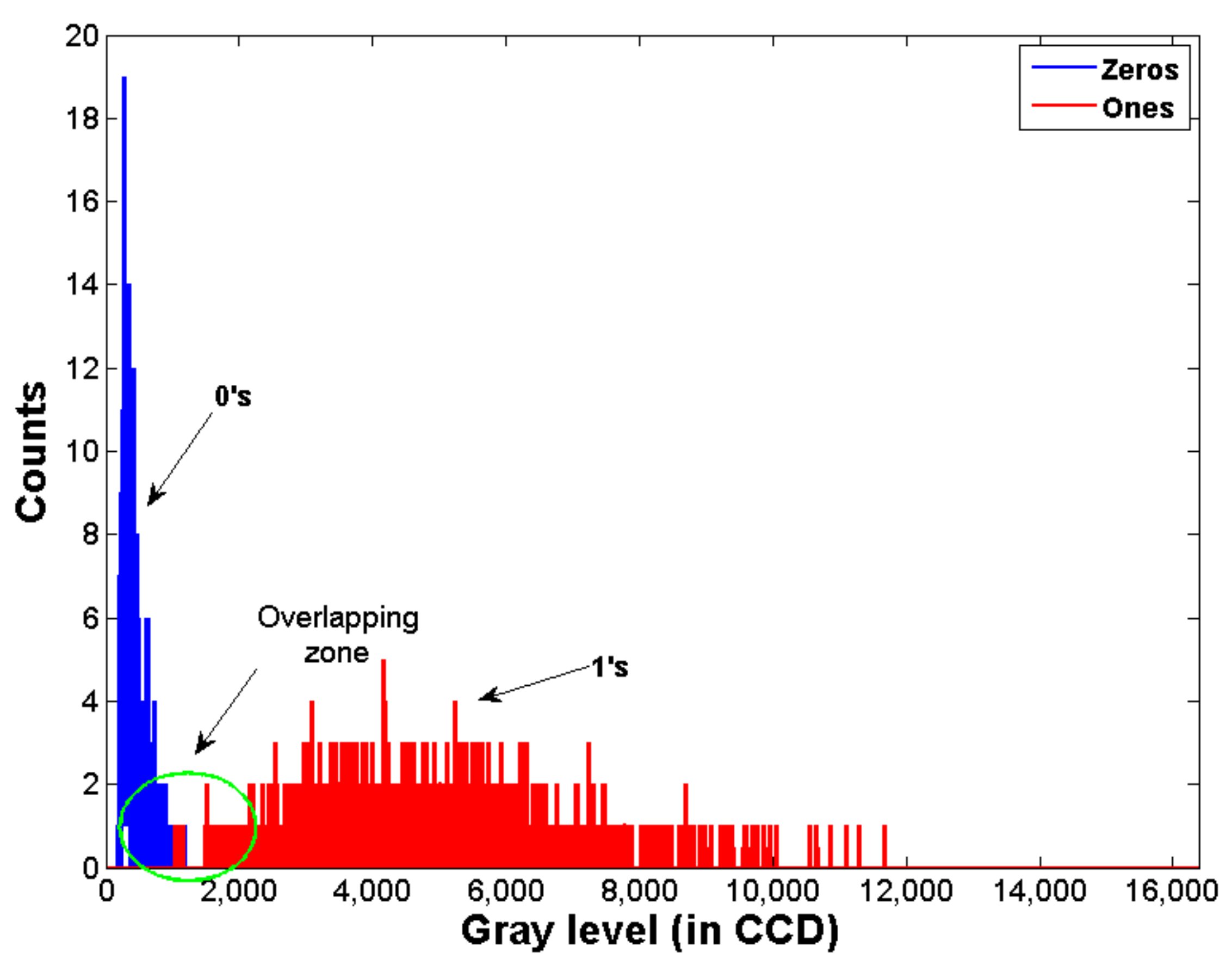
To calculate the Q-factor in Equation (1), which permits us a more reliable BER calculation, we needed more statistical information. To use this figure of merit, we divided into bits the original image, before applying any threshold on it, and we associated the gray level with the position of an ON or an OFF state (1 or 0). Then, we took the value measured by the CCD and countrf the number of bits at that level.
Figure 6 shows the distribution of the different gray levels where we have identified the ON and OFF states. We see that there is a zone where the histograms of levels ON and OFF overlap. This zone contains the best level to threshold the image to minimize the number or errors. The extension of the zone, where the states overlap, also defines the number of errors that we encounter in the analysis.
4. Results
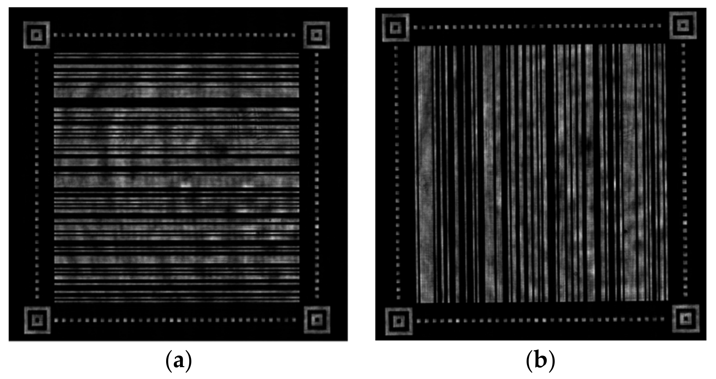
In this section, we present the results for the different images obtained. As we have mentioned, we used bit aggregates in the shape of linear stripes oriented vertically and horizontally to test the anamorphic effects. In addition, we changed the resolution in the image displayed: we used as information unit a group of pixels in the PA-LCoS. In
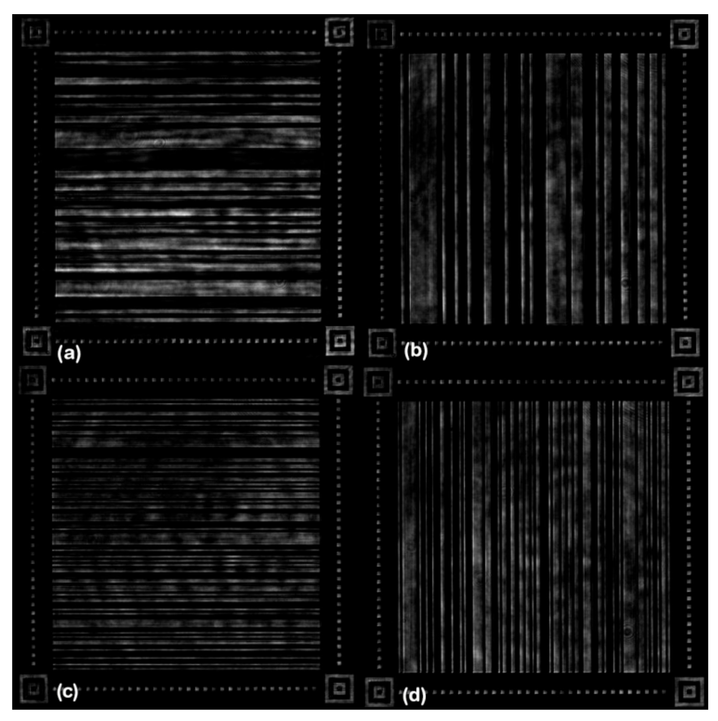
Figure 7, we plot the images captured by the CCD camera when addressing the stripe data shape onto the PA-LCoS, respectively, for horizontal and vertical orientation for a bit size of 4 × 4 pixels. These are the original images before the thresholding operation.
The first thing to notice is the irregular illumination observed. This produces and image where a unique threshold level for the entire image does not exist. As we can vary the threshold level to make an image binarization, we can obtain some figures of merit to analyze the irregular illumination observed, and we can calculate the number of errors for all the threshold levels considered.
The images depicted in
Figure 7 are the ones captured by our CCD camera with a bit depth of 14 bits, so we have 16,384 possible gray levels. As long as we avoid saturating the CCD, we do not need to consider a full variation of all levels when we try to seek for the best threshold level. It is usually enough to consider a variation of 6000 levels, which is more than the typical extent of the overlapping zone (see
Figure 6).
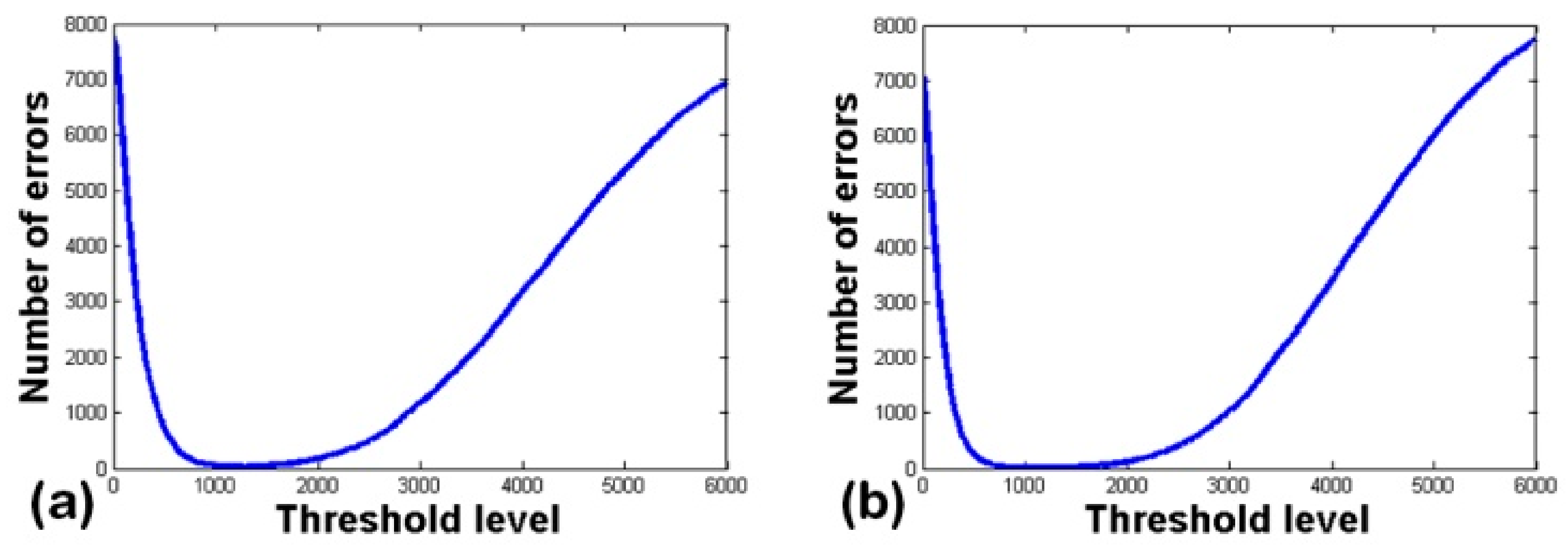
Figure 8 presents the evolution in the number of errors counted as a function of the threshold level. The graph width gives us an idea about how sensitive is the information reconstruction to the threshold level. In fact, we observe how the number of errors decreases to a minimum and then rises again. The minimum level of light is not zero, since there always exists a thermal noise or a residual light intensity, thus it will be enough to start analyzing from a threshold level greater than 100, in our case we consider 200. The best threshold level would be the one that minimizes the number of errors. To be sure that we have selected the best threshold, we have to obtain a curve with an evolution, as the one reflected in either
Figure 8a,b, which means that the number of error decreases until a minimum point and then the number of error rises again. That shape means that we have selected a range large enough to contain the threshold level that minimizes the number or errors.
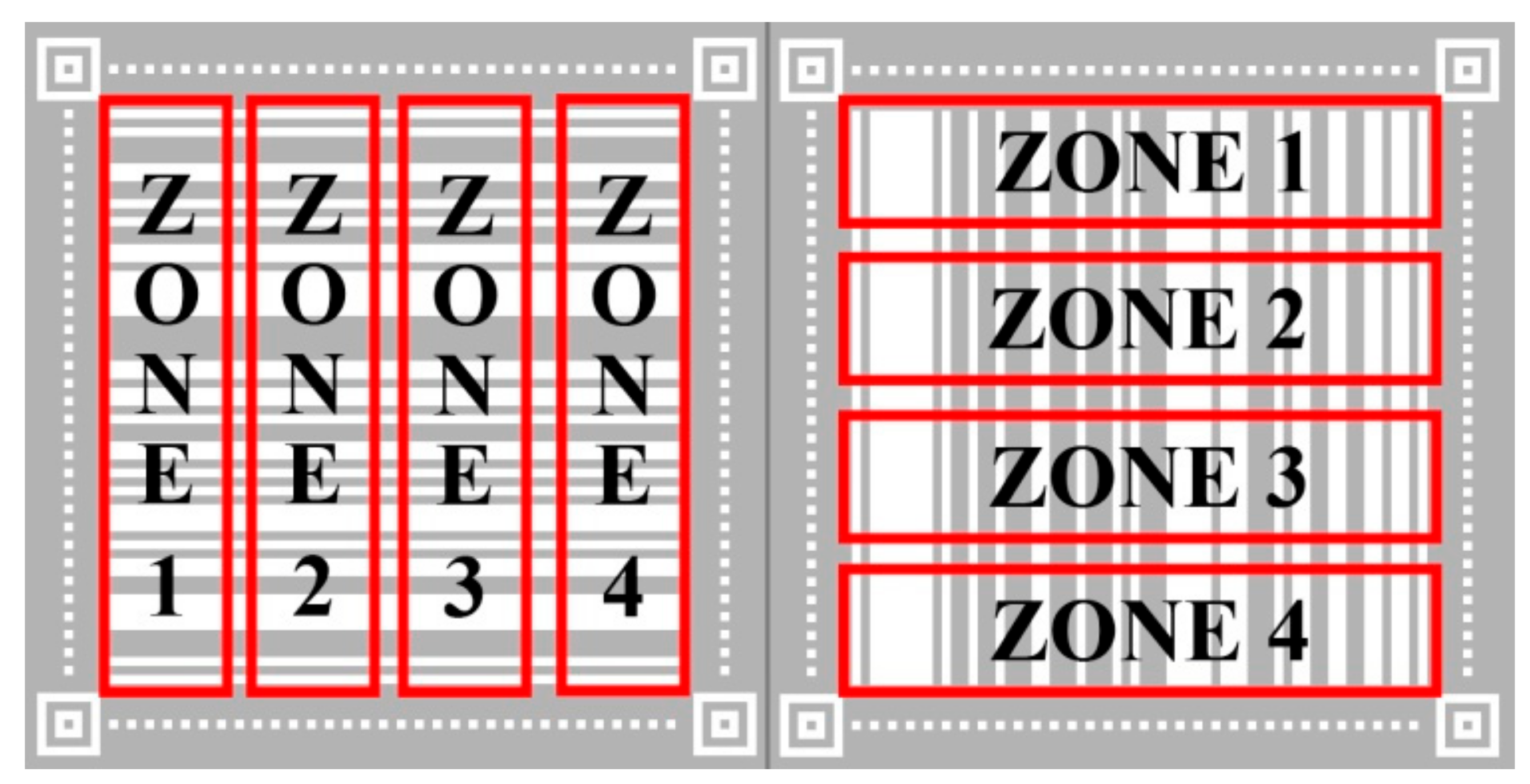
To analyze the illumination influence, we now divide the image into four zones. Each of them can be analyzed in the same way described for the full image. In
Figure 9, we show how we have defined the zones for the different orientations. Each zone is a different set of data to extract statistical results, as presented in the previous section.
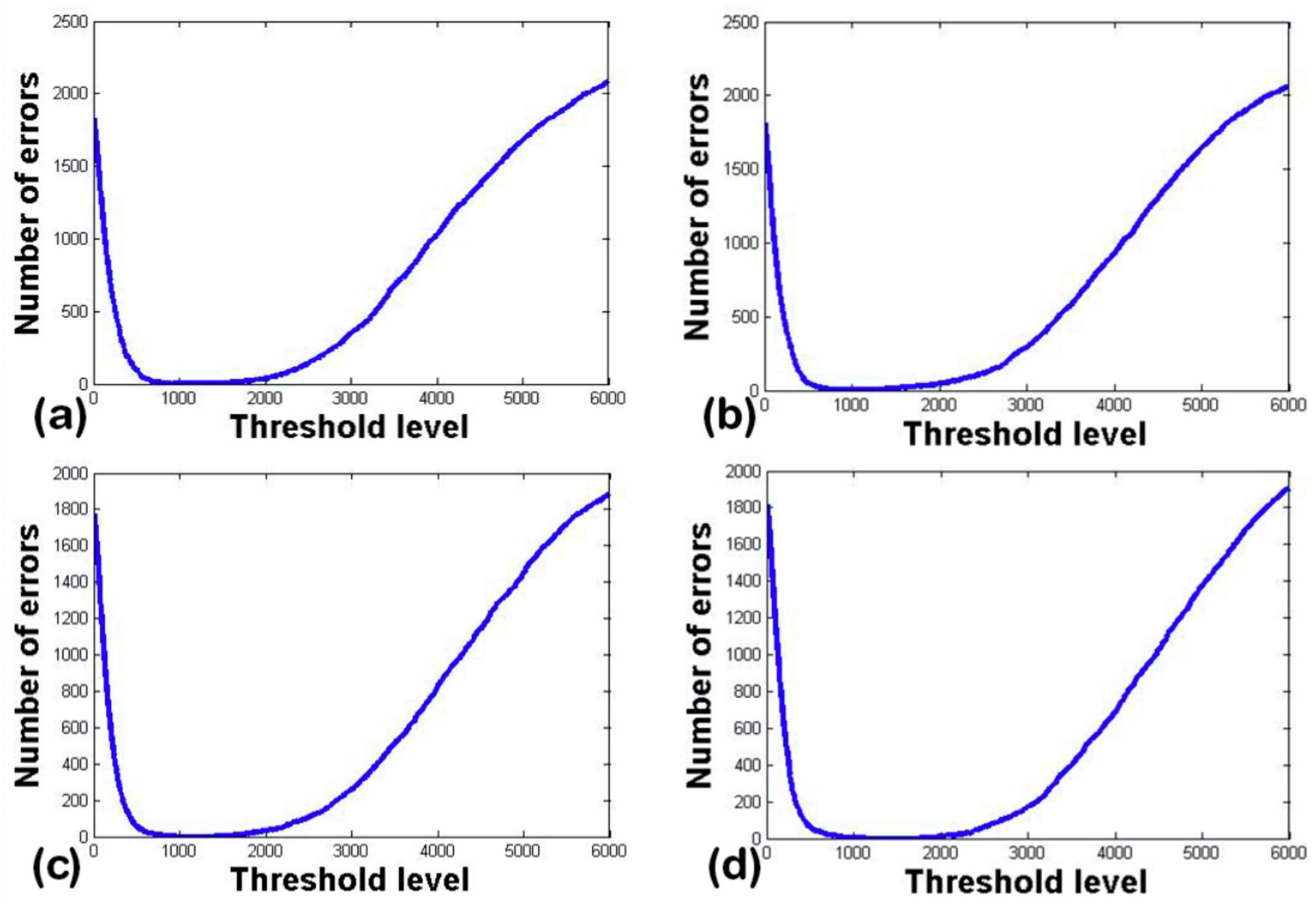
Figure 10 shows the different graphs for the zones defined in
Figure 9 for vertical stripes. These zones have the same shape, but we can observe that they have slightly different best threshold levels for every zone. As long as the graph shape is preserved, the differences do not produce a significant increase in the number of errors.
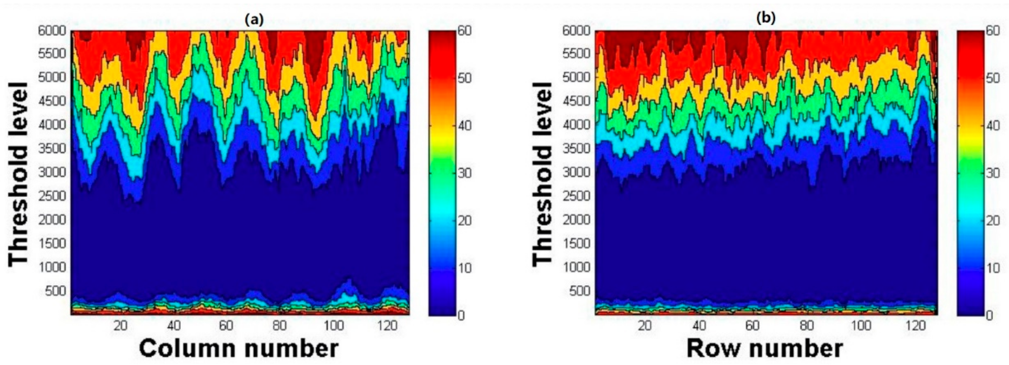
To maintain the possibility to compute statistical results, we do not reduce the size of the zones to look for illumination inhomogeneities. Reducing the size of the zones decreases the number of information bits available to calculate histograms. Nevertheless, as a qualitative evaluation tool, we have calculated the number of errors for every column (horizontal stripes) or row (vertical stripes). In this way, we see that there are columns (or rows) in which we identify all 0s and 1s correctly. This kind of graphs allows us to study and evaluate the illumination, but it is not statistically significant to calculate Q-factor or BER per row (or column), because we only have 128 bits of data for each column or row in an image that use 4 × 4 pixels per bit. In the best case, we would have 512 bits per column when using 1 × 1 pixel per bit.
In
Figure 11, the number of errors is pseudocolored: blue represents few errors than red. We show the number of errors detected in a specific column in
Figure 11a (row in
Figure 11b). The column number is represented in the X-axis (when we use vertical stripes, this number refers to a specific row), and the evolution in the number of errors as a function of the threshold level is represented in the Y-axis. This representation gives us some clues about the illumination and how sensitive is the threshold level selection. A wider blue zone, which is correlated with the large valley in
Figure 8, implies that the selection of the threshold level is less critical. The ripples shown in
Figure 11 come from the illumination inhomogeneities: we can see that the horizontal orientation (
Figure 11a) is more sensitive to these inhomogeneities.
For the different bit sizes and linear stripes orientations, we provide specific quantitative results in tabular form.
Table 1 and
Table 2 shows the data page as a whole, and
Table 3 and
Table 4 shows them in terms of the local characterization in four regions across the aperture of the data page.
First, in
Table 1 and
Table 2, we show the measured Q-factor and BER for the different bit sizes and orientations considered. The Q-factor is calculated using Equation (1), and the data were obtained from the histograms (
Figure 8 and
Figure 10). The BER was obtained applying Equation (2). We have also included the number of errors, counting directly, associated with the optimum threshold level. The first thing that we note is that the bit size of 2 × 2 pixels presents a very high BER and a low Q-factor. This is because this bit size is in the resolution limit of our system, as we calculated from the 1951 USAF resolution test target shown in
Figure 2. Therefore, this resolution is out of our scope due to the limitations imposed by the optical system, not to the LCoS display.
Table 1 also reflect that the BER is in the order of 10
−3 or below before introducing error correction codes. This fact indicates that the reconstruction without errors is possible [
28,
29].
From the results in
Table 1 and
Table 2, we also see that the Q-factor and BER values are better, i.e., less image degradation, for the vertical stripes images. This contradicts the results in diffractive optical elements displayed on LCoS devices [
8,
10,
11] where diffraction efficiency becomes smaller for vertically oriented elements, i.e., periodicity along the columns of the LCoS. One possible explanation for this difference is that in the HDSS application in the paper, where BIM data pages are introduced, there is wider tolerance to the anamorphic effects introduced by LCoS devices. Now, we do not display periodic diffractive elements and the figure of merit is not diffraction efficiency. In our present case, the binary intensity contrast between the ON and OFF levels in the LCoS is the important magnitude and this has a limited dependency with the orientation of the non-periodic stripes displayed.
We divided the data image into various zones, as presented in
Figure 9, to analyze the Q factor and the BER by zones. This kind of analysis helps us to detect problems in the uniformity of the illumination, or errors due to deformations in the image.
In
Table 3 and
Table 4, we show the Q-factor obtained in the different zones. In horizontal stripes (
Table 3), Zone 1 corresponds to the left part on the image. We observe that. for every bit size. the worst Q-factor is obtained in Zone 3. Nevertheless, for vertical stripes (
Table 4), we see that the Q-factor decreases with the number of the zone, that means from top to the bottom (
Figure 9, left). This kind of analysis allows us to measure the illumination inhomogeneity: if the difference is too high, we would have to improve the experimental setup to avoid this source of error.
We present results for the complete reconstruction process. When we introduce the photopolymer, new distortion elements appear. The manufacturing process can introduce ripples and deformations due to continuous exchange of water molecules between material and environment. In addition, the natural crystallization may affect the recording process [
32].
In
Figure 12, we show the image captured by the CCD during the reconstruction process. We show the reconstructed images for the 8 × 8 and 4 × 4 bit sizes to compare with the results obtained without material. The degradation effects increase the BER, and lower the Q-factor accordingly, as can be observed in
Table 5 and
Table 6, for the analysis of the reconstructed data pages with the horizontal (
Table 5) and vertical patterns (
Table 6) with the recording material.
Comparing the results in
Table 5 and
Table 6, when the material is introduced, with the corresponding results in
Table 1 and
Table 2, we see that the number of errors increases by one order of magnitude, which makes the resolutions under a pixel size of 4 × 4 out of the values that can be recovered with an error correction code. Perhaps, the non-uniformity illumination is influencing in the registration process, but it is even more likely that slight non-uniformity in the deposition of the material has a relevant role in the degradation of the BER.
We expect that the BER obtained for a single hologram will not be affected by multiplexing as long as the Bragg selectivity (in the case of angular multiplexing) is maintained, as long as we do not saturate the dynamic range of the material and maintain an appropriate relation between diffraction efficiency and the number of holograms stored [
33].
5. Conclusions
In this paper, we present a method to discover the limits of an Holographic Data Storage System, with an emphasis on the existence of anamorphic and frequency dependent effects due the PA-LCoS microdisplay. We defined two figures of merit to evaluate the possibilities of doing an exact reconstruction: Q-factor and BER.
We discovered that the anamorphic effect does not influence the results when a non-periodic pattern is used. This effect seems to have an influence when we used periodic diffractive optical elements [
34]. We evaluated two figures of merit, BER and Q-factor, exposed in Equations (1) and (2), which serve to predict that, without using recording material, we can reconstruct data pages with a resolution of 3 × 3 pixels per bit in a reliable way. The fact that the BER is in the order of 10
−3 or below indicates that our HDSS can be used to store and retrieve data with a high data density.
The different graphs that we obtain with this characterization method also allow us to see illumination problems that have to be solved to improve the performance. To do that, we divided the image into four zones. This local evaluation can be done without adding elements to the experimental setup. We can also extract qualitative information about illumination by analyzing the image column by column (or row by row). We consider that the method is easy to implement and useful to detect limitations and problems in Holographic Data Storage Systems in a systematic way.
We analyzed the BER when the holographic material is introduced and, despite the increased number of errors, the BER is good enough to consider that the data can be recovered. However, we need to improve the homogeneity in the material deposition, or even try to use a commercial material such as Bayfol
®, which is made industrially and is protected with a film that prevents material degradation and guaranties uniformity [
35].

 ,
, 


