Bi-Level Planning Model of Charging Stations Considering the Coupling Relationship between Charging Stations and Travel Route

 ,
, 
Abstract
:
1. Introduction
- -
- In this study, we consider the coupling relationship between EV users’ travel routes and the location of charging stations. The shortest path would be the best choice, however, when it could cannot meet the traveling demand, we search other routes passing the fast charging stations within a certain deviation so as to analyze the trip feasibility.
- -
- In order to simulate the process of users heading for charging stations to charge, we accord priority consideration to charging when the state of charge (SOC) is less than the range anxiety threshold, and then to charge on relatively sufficient battery. Following this method, we obtain the number of EVs charged at each station, which enables us to achieve a more reliable and practical sizing result.
- -
- Based on the charging times and deviation, we propose the concept of the satisfaction index. The satisfaction index can reflect the convenience that the location of the charging stations would bring to the users.
- -
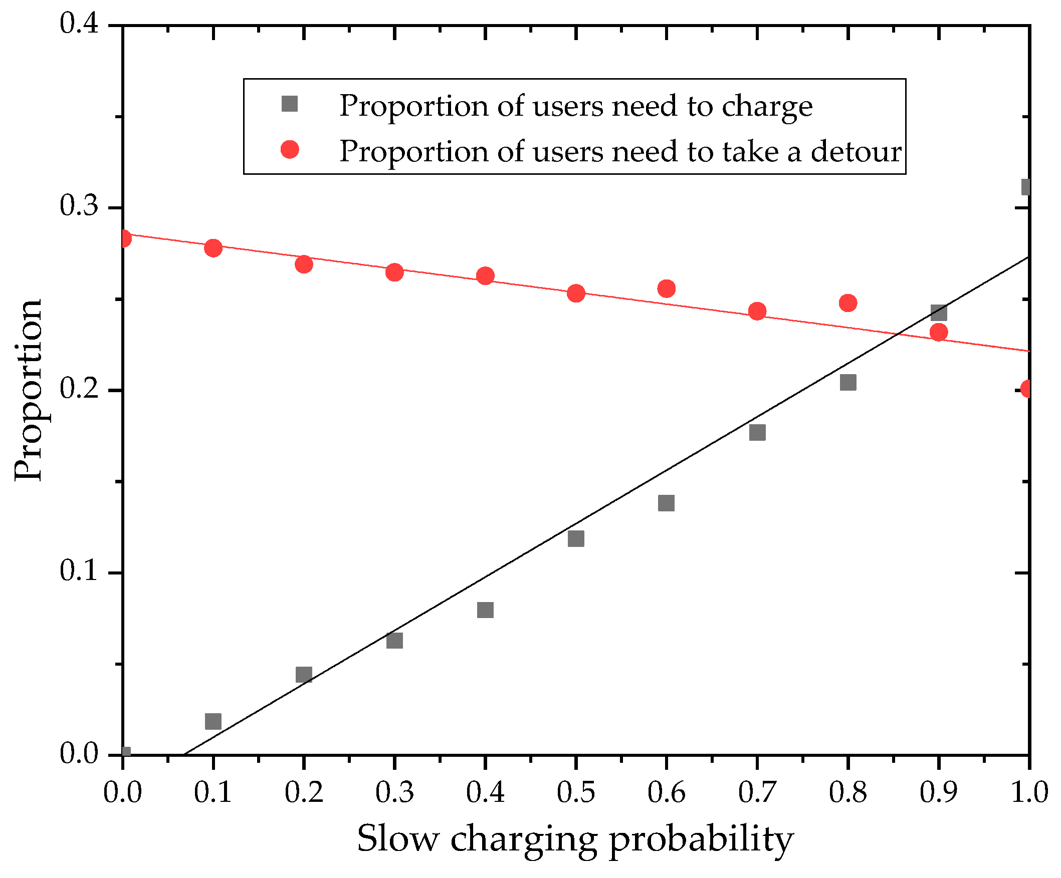
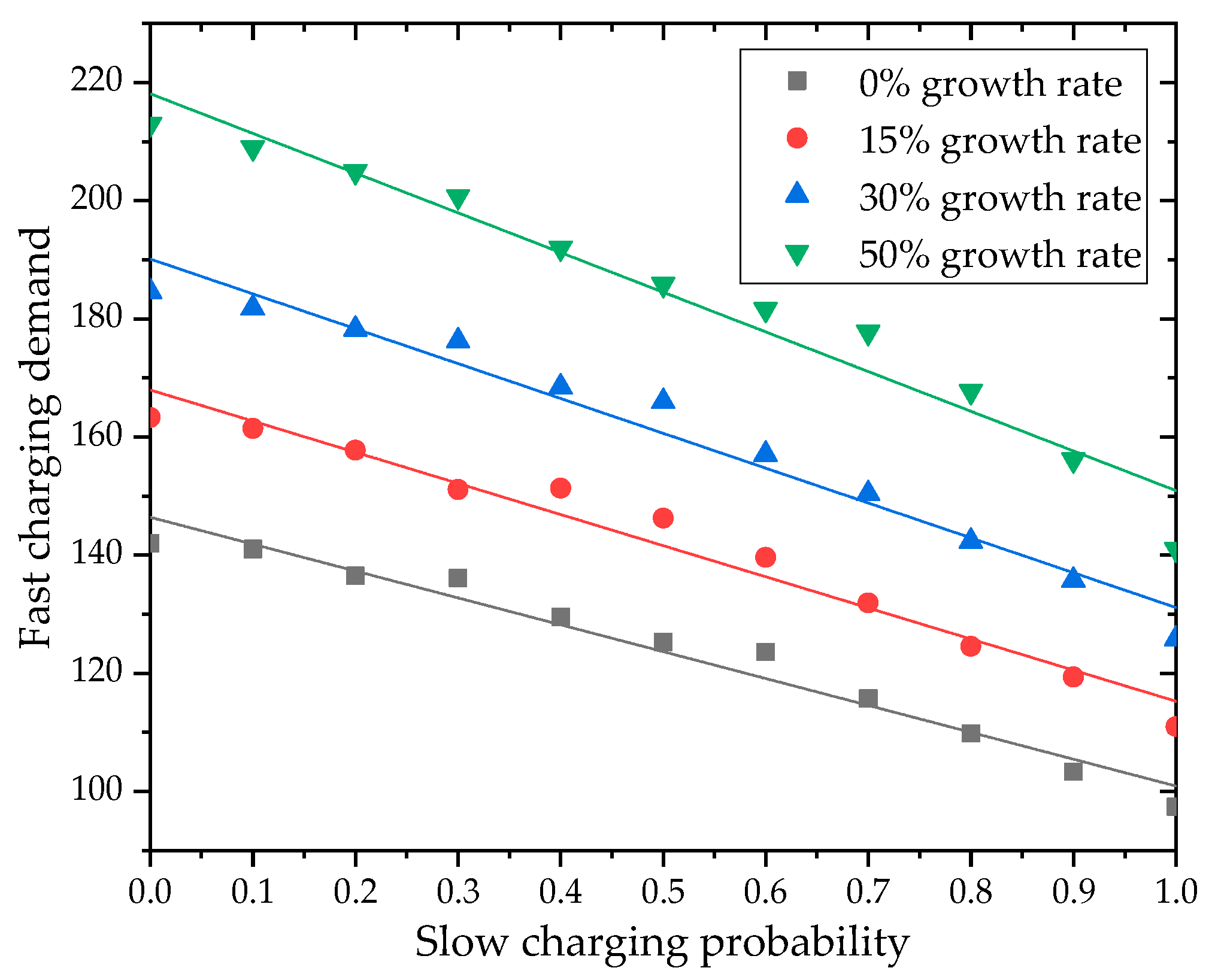
- In this research, we combine slow charging in the public parking lot and fast charging in the fast charging station, and research the impact of the increase of EV ownership and coverage of slow chargers on the fast charging demand and the travel success ratio.
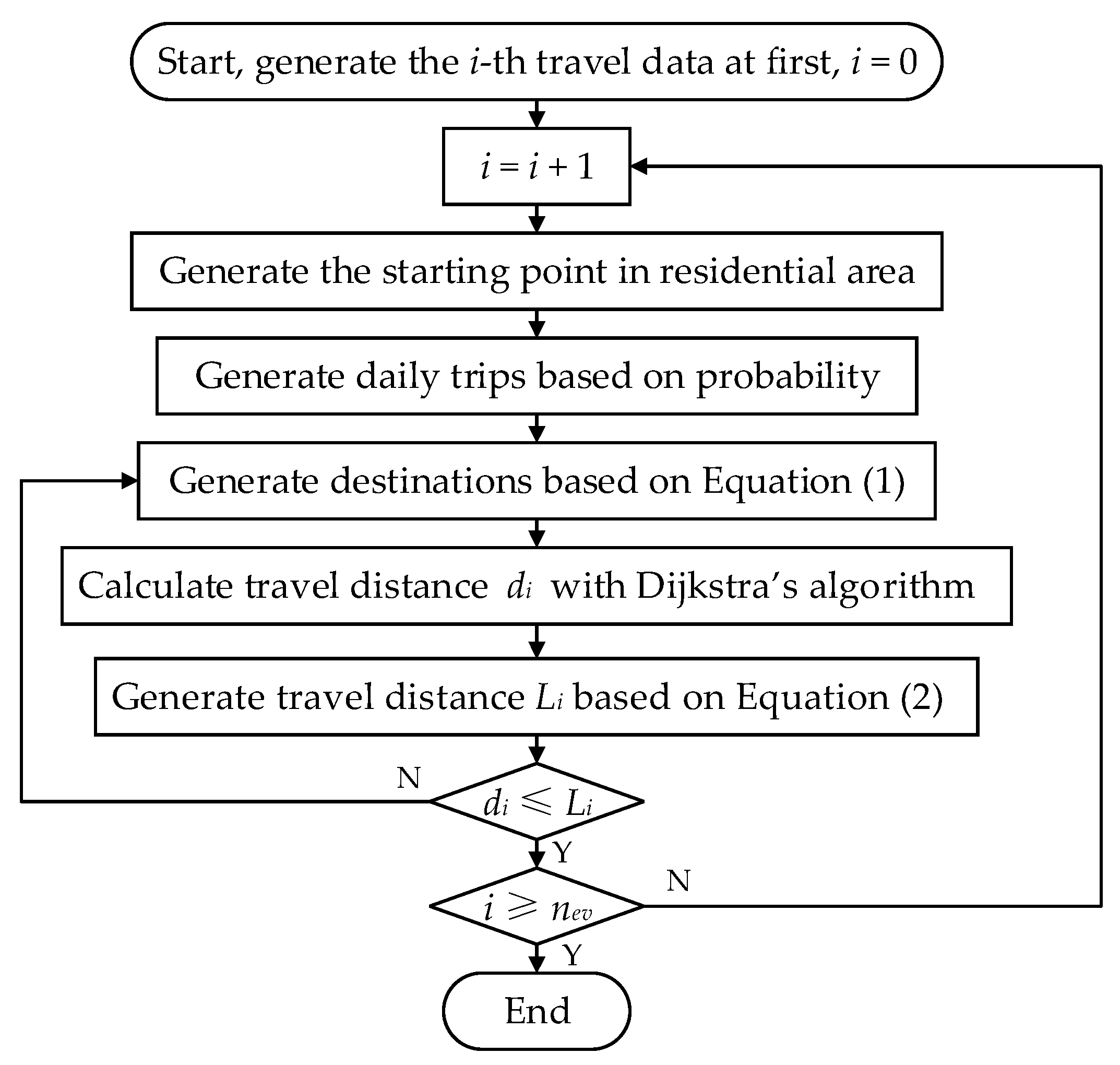
2. Uncertainty Modeling of Travel Pattern
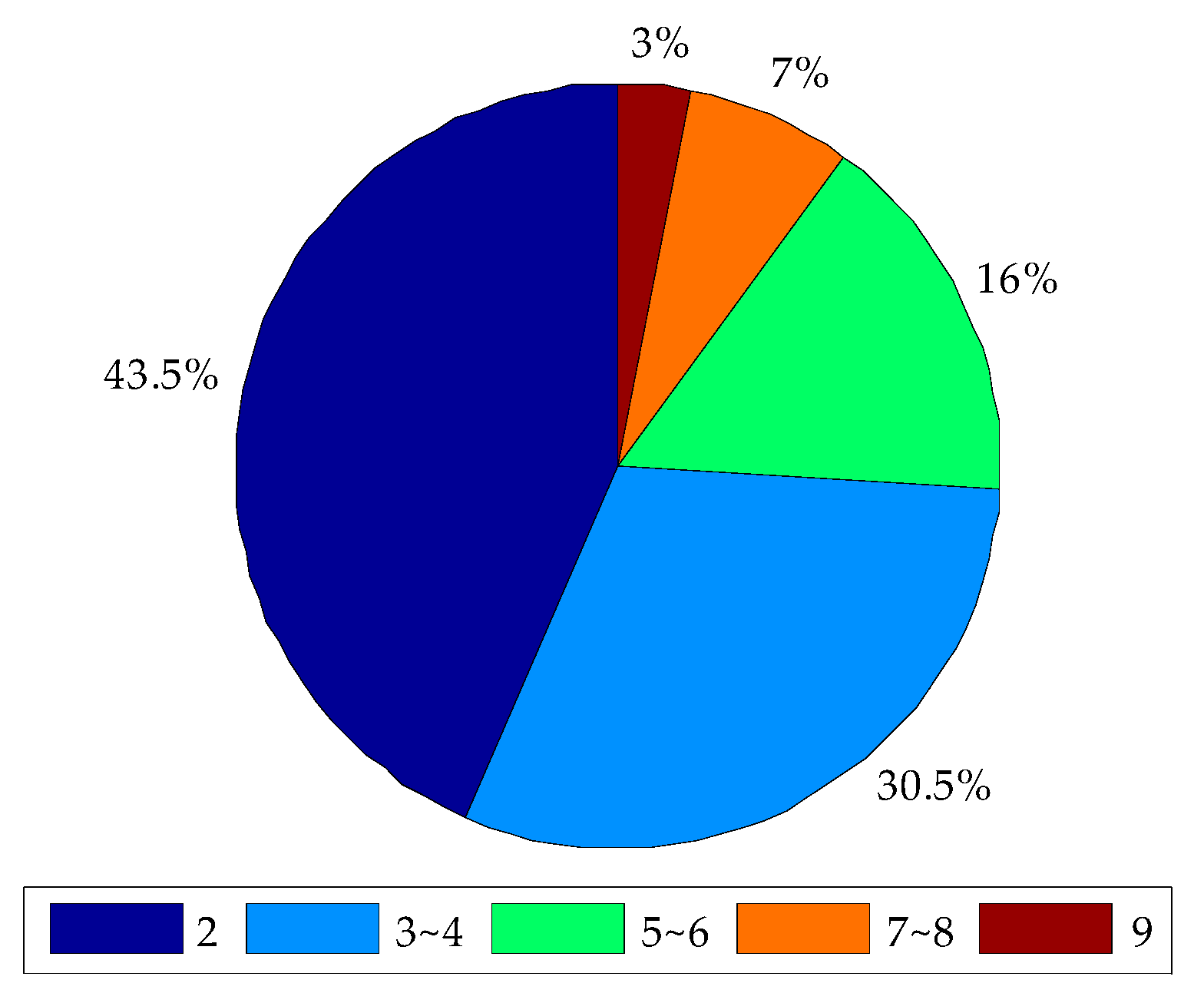
2.1. Daily Trips
2.2. Destination of Trip
2.3. Travel Distance
3. Coupling Relationship between Charging Stations and Travel Route
3.1. Impact of Charging Stations on Travel Route
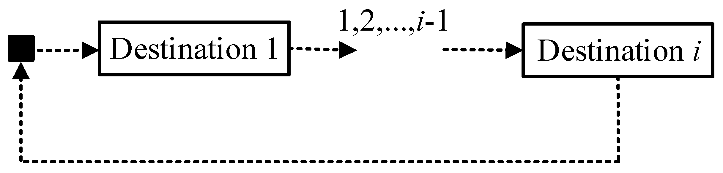
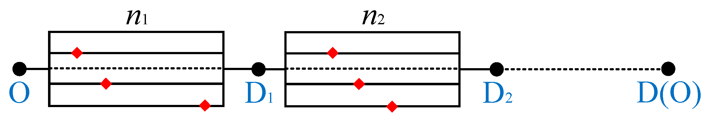
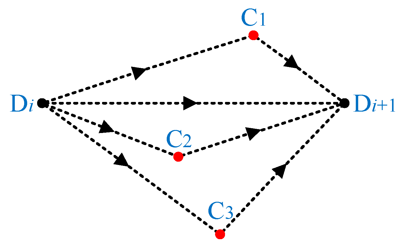
3.2. Potential Trip Chains Considering the Location of Charging Stations
3.3. Feasibility Analysis of Trip Chains
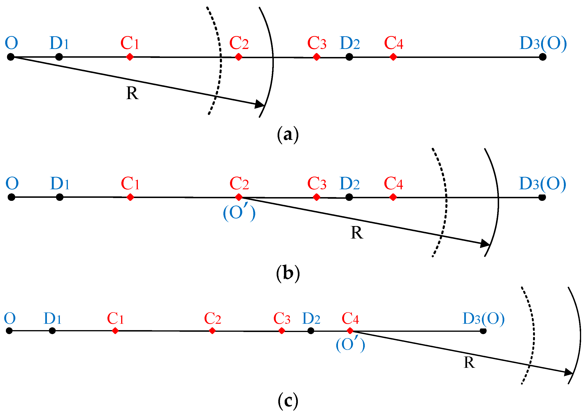
- When d ≤ R which indicates that the traveling distance is smaller than the maximum travel range of EVs, charging is not necessary, thus the trip is a success; and
- When d > R which indicates that the traveling distance exceeds the maximum travel range of EVs, charging is necessary and we need to the judge whether the trip is a success and analyze which charging station(s) the user needs to charge at.
- If there is no charging station found in the range of (0,R), the user cannot reach the next destination. The trip chain is deemed a failure.
- If there are any charging stations found in the range of (R’,R), we will opt for the charging station closer to the start point. As the battery runs at a lower level, the user will become anxious and choose to charge immediately.
- If there are any charging stations found in the range of (0,R’), we will choose the charging station farthest from the starting point. As the vehicle could still provide sufficient power, the charging demand is not that urgent. The time cost in the charging station would be lower for the user and she/he could charge more if she/he charges at a low-power state, thus, leading to a higher probability of a successful trip.
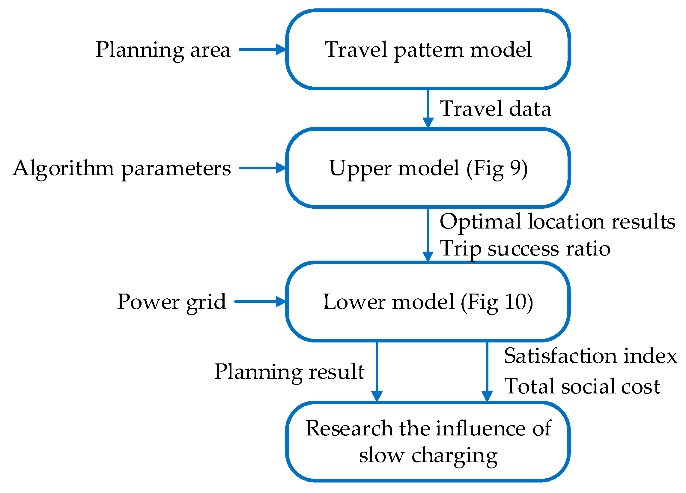
4. Upper Model Based on the Travel Success Ratio
4.1. Model Formulation
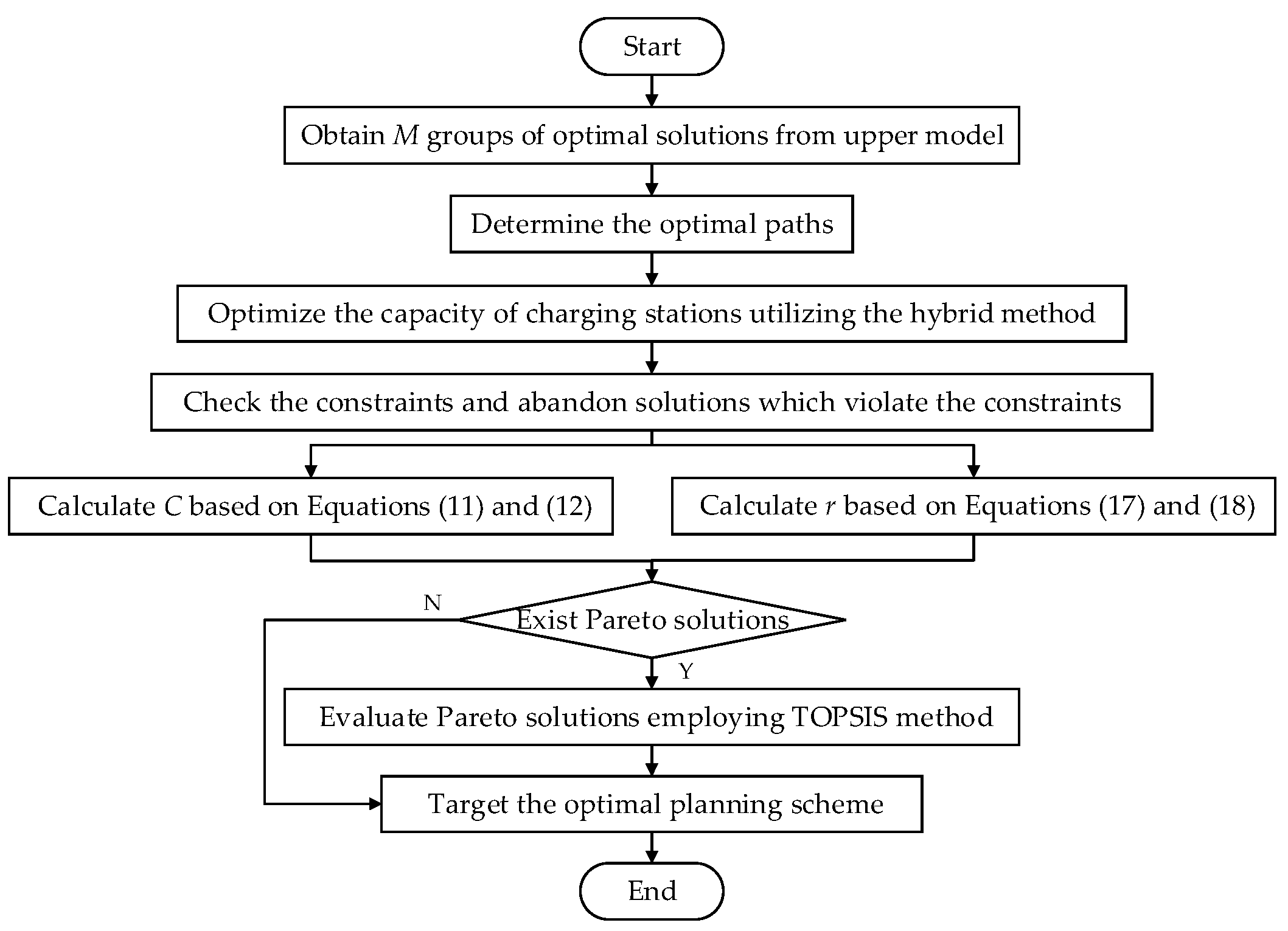
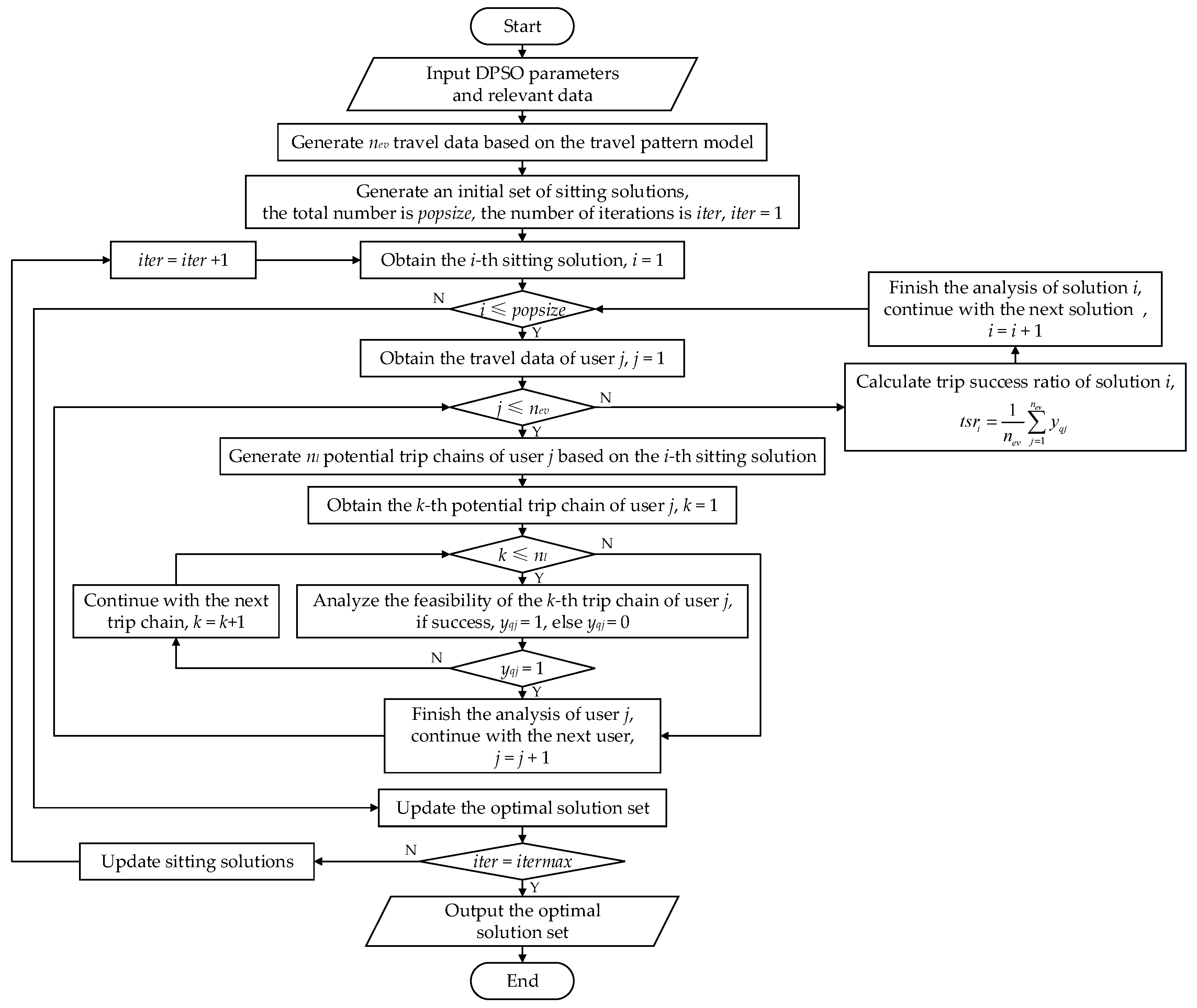
4.2. Solution Method
5. Lower Model Based on the Satisfaction Index and Total Social Cost
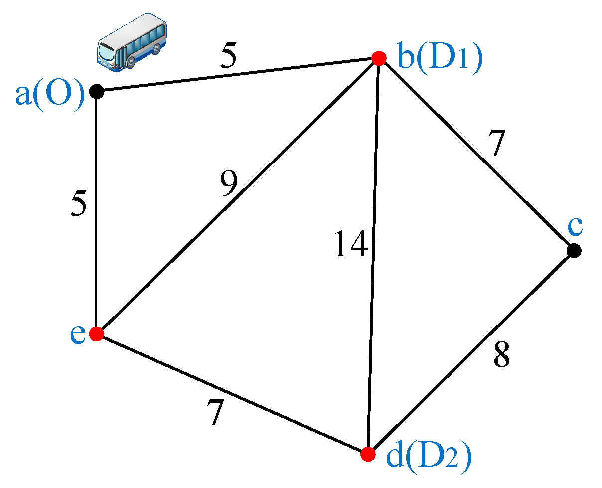
5.1. Determination of the Optimal Path
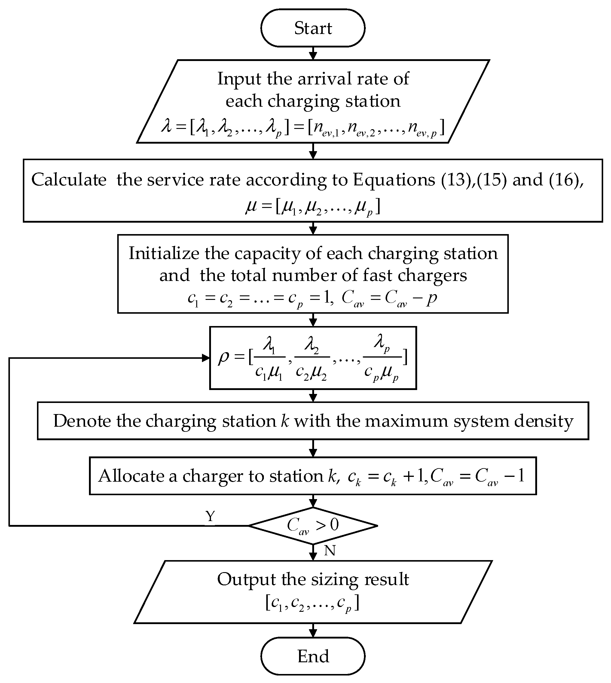
5.2. Sizing Model Based on the Hybrid Method
5.3. Grid Constraints
5.4. Satisfaction Index
5.5. Total Social Cost
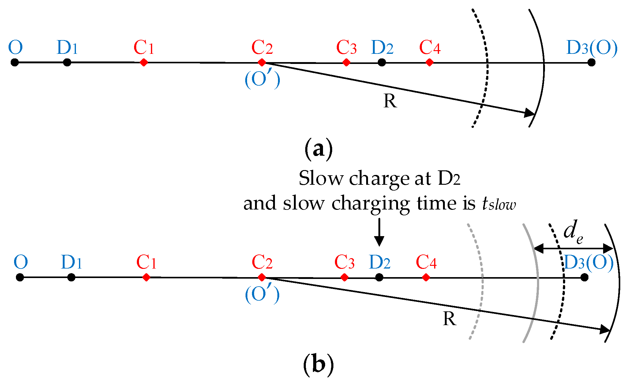
6. Feasibility Analysis Considering Slow Charging at Destinations
7. Case Study
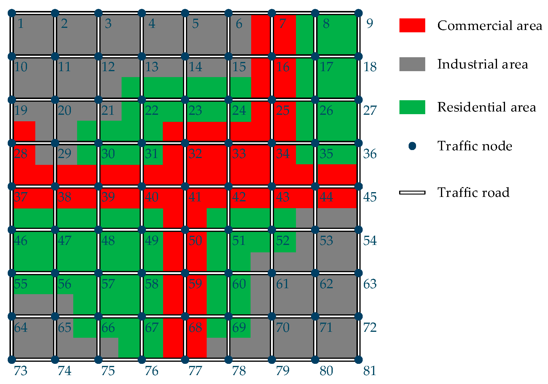
7.1. Planning Area
7.2. Simulation Results Considering Only Fast Charging
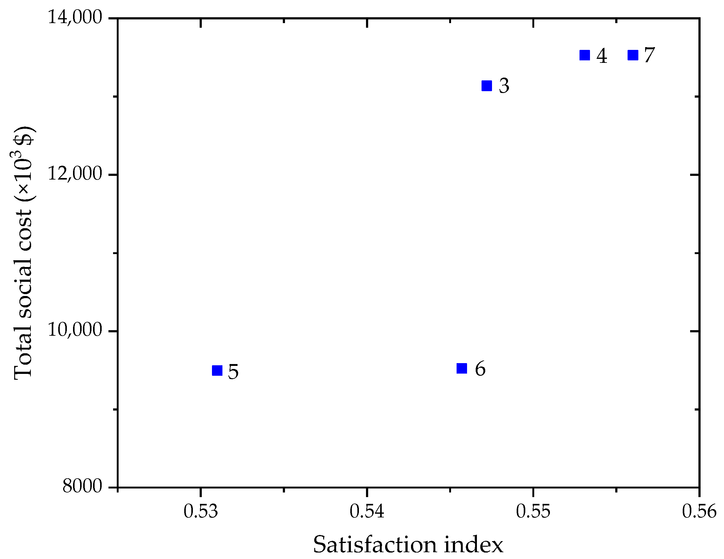
7.3. Simulation Results Using FCLM
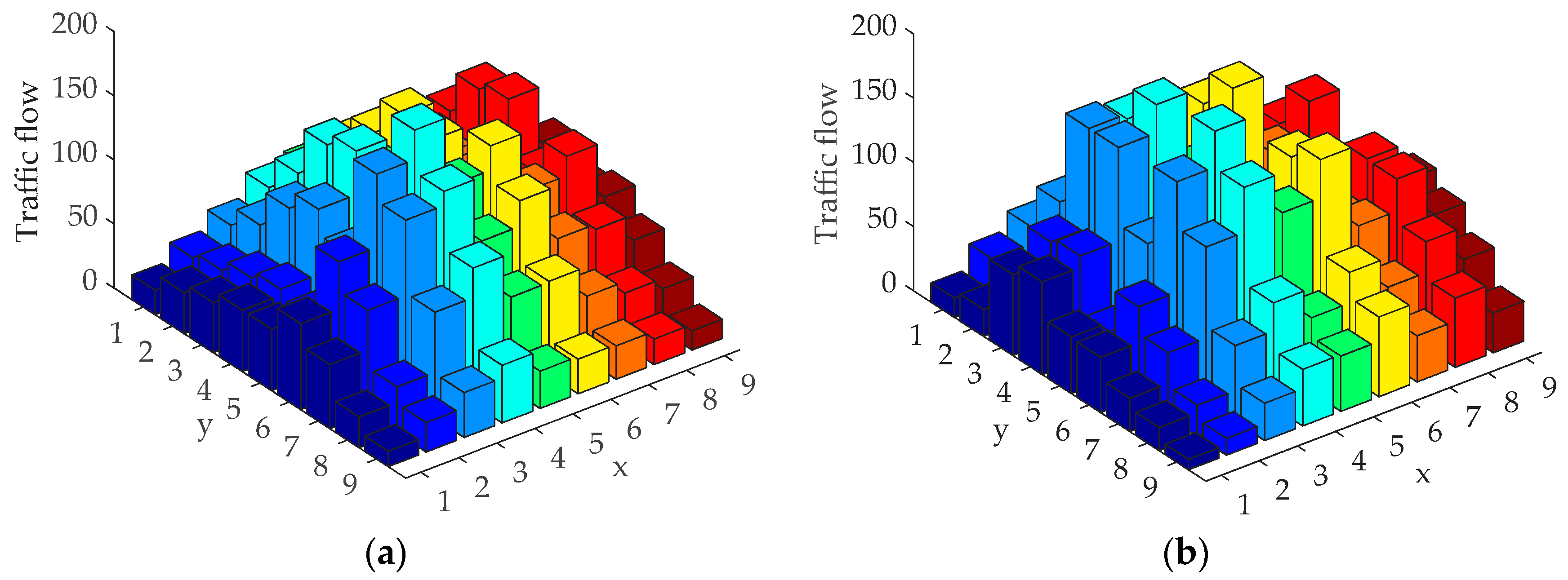
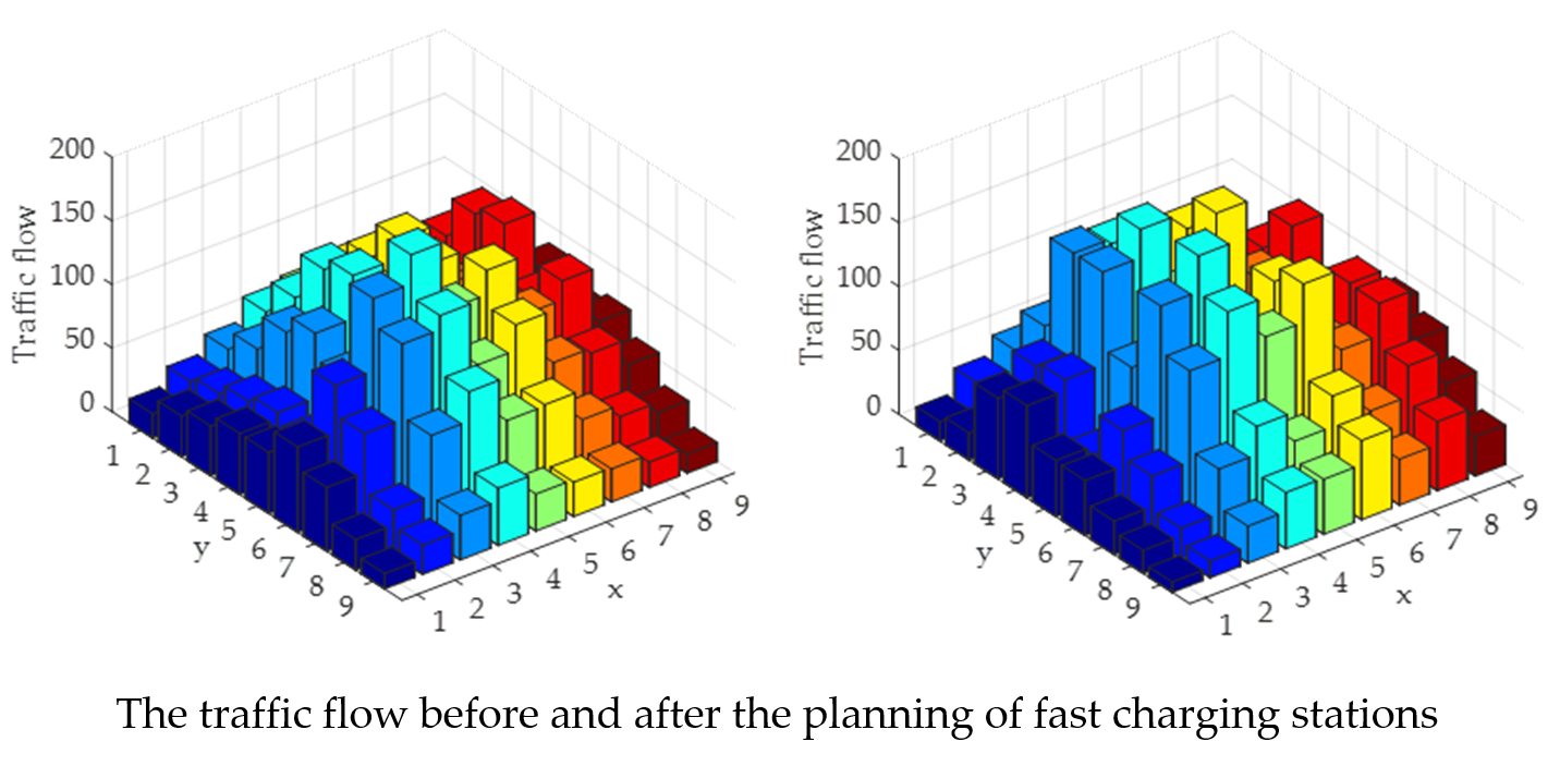
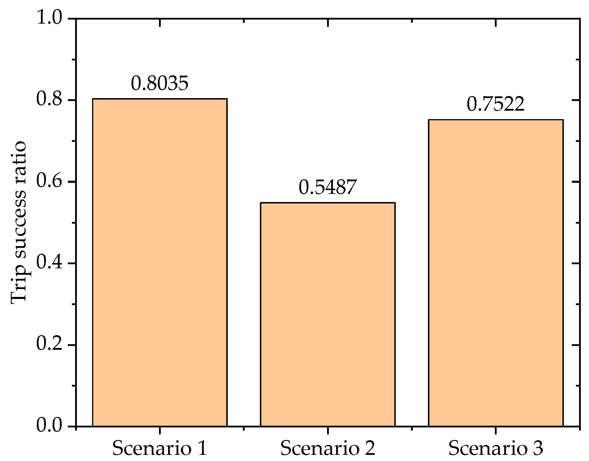
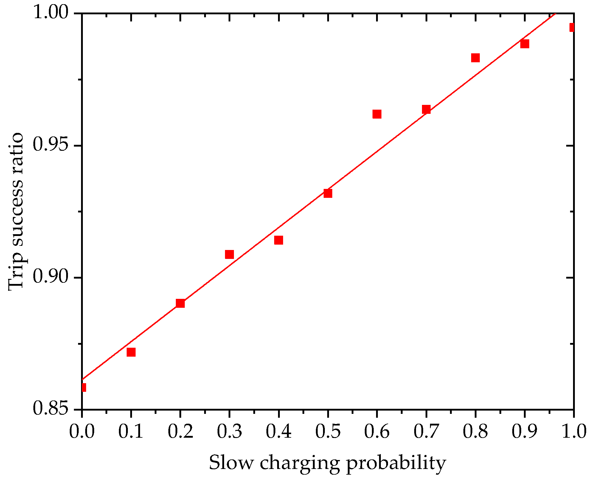
7.4. Simulation Results Considering Slow Charging at Destinations
8. Conclusions
Author Contributions
Funding
Conflicts of Interest
References
- Chen, Q.; Liu, N.; Wang, C.; Zhang, J. Optimal power utilizing strategy for pv-based ev charging stations considering real-time price. In Proceedings of the 2014 IEEE Conference and Expo Transportation Electrification Asia-Pacific (ITEC Asia-Pacific), Beijing, China, 31 August–3 September 2014; pp. 1–6. [Google Scholar]
- U.S. Environmental Protection Agency. Greenhouse Gas Emissions from the U.S. Transportation Sector: 1990–2003. Available online: http://www.epa.gov/otaq/climate/420r06003.pdf (accessed on 18 April 2018).
- Christensen, T.B.; Wells, P.; Cipcigan, L. Can innovative business models overcome resistance to electric vehicles? Better place and battery electric cars in denmark. Energy Policy 2012, 48, 498–505. [Google Scholar] [CrossRef]
- Aziz, M.; Oda, T. Simultaneous quick-charging system for electric vehicle. Energy Procedia 2017, 142, 1811–1816. [Google Scholar] [CrossRef]
- Nie, Y.; Ghamami, M.; Zockaie, A.; Xiao, F. Optimization of incentive polices for plug-in electric vehicles. Transp. Res. Part B 2016, 84, 103–123. [Google Scholar] [CrossRef]
- Kontou, E.; Yin, Y.; Lin, Z.; He, F. Socially optimal replacement of conventional with electric vehicles for the us household fleet. Int. J. Sustain. Transp. 2017, 11, 749–763. [Google Scholar] [CrossRef]
- Singer, M. Consumer Views on Plug-In Electric Vehicles—National Benchmark Report; National Renewable Energy Laboratory: Golden, CO, USA, 2016. [Google Scholar]
- Aziz, M.; Oda, T.; Mitani, T.; Watanabe, Y.; Kashiwagi, T. Utilization of electric vehicles and their used batteries for peak-load shifting. Energies 2015, 2015, 3720–3738. [Google Scholar] [CrossRef]
- Lojowska, A.; Kurowicka, D.; Papaefthymiou, G.; Lou, V.D.S. Stochastic modeling of power demand due to evs using copula. IEEE Trans. Power Syst. 2012, 27, 1960–1968. [Google Scholar] [CrossRef]
- Mu, Y.; Wu, J.; Jenkins, N.; Jia, H.; Wang, C. A spatial–temporal model for grid impact analysis of plug-in electric vehicles. Appl. Energy 2014, 114, 456–465. [Google Scholar] [CrossRef]
- Liang, H.; Sharma, I.; Zhuang, W.; Bhattacharya, K. Plug-in electric vehicle charging demand estimation based on queueing network analysis. In Proceedings of the Pes General Meeting | Conference & Exposition, National Harbor, MD, USA, 27–31 July 2014; pp. 1–5. [Google Scholar]
- Bae, S.; Kwasinski, A. Spatial and temporal model of electric vehicle charging demand. IEEE Trans. Smart Grid 2012, 3, 394–403. [Google Scholar] [CrossRef]
- Andrenacci, N.; Ragona, R.; Valenti, G. A demand-side approach to the optimal deployment of electric vehicle charging stations in metropolitan areas. Appl. Energy 2016, 182, 39–46. [Google Scholar] [CrossRef]
- Dong, X.; Mu, Y.; Jia, H.; Wu, J.; Yu, X. Planning of fast ev charging stations on a round freeway. IEEE Trans. Sustain. Energy 2016, 7, 1452–1461. [Google Scholar] [CrossRef]
- Ip, A.; Fong, S.; Liu, E. Optimization for allocating bev recharging stations in urban areas by using hierarchical clustering. In Proceedings of the International Conference on Advanced Information Management and Service, Seoul, Korea, 30 November–2 December 2010; pp. 460–465. [Google Scholar]
- Frade, I.; Ribeiro, A.; Gonçalves, G.; Antunes, A.P. Optimal location of charging stations for electric vehicles in a neighborhood in Lisbon, Portugal. Transp. Res. Rec. J. Transp. Res. Board 2011, 2252, 91–98. [Google Scholar] [CrossRef]
- Sadeghi-Barzani, P.; Rajabi-Ghahnavieh, A.; Kazemi-Karegar, H. Optimal fast charging station placing and sizing. Appl. Energy 2014, 125, 289–299. [Google Scholar] [CrossRef]
- Xiang, Y.; Liu, J.; Li, R.; Li, F.; Gu, C.; Tang, S. Economic planning of electric vehicle charging stations considering traffic constraints and load profile templates. Appl. Energy 2016, 178, 647–659. [Google Scholar] [CrossRef] [Green Version]
- Wang, G.; Xu, Z.; Wen, F.; Wong, K.P. Traffic-constrained multiobjective planning of electric-vehicle charging stations. IEEE Trans. Power Deliv. 2013, 28, 2363–2372. [Google Scholar] [CrossRef]
- Berman, O.; Larson, R.C.; Fouska, N. Optimal location of discretionary service facilities. Transp. Sci. 1992, 26, 201–211. [Google Scholar] [CrossRef]
- Hodgson, M.J. A billboard location model. Geogr. Environ. Modeling 1997, 1, 25–45. [Google Scholar]
- Hodgson, M.J. A flow-capturing location-allocation model. Geogr. Anal. 2010, 22, 270–279. [Google Scholar] [CrossRef]
- Wang, S.; Dong, Z.Y.; Luo, F.; Meng, K.; Zhang, Y. Stochastic collaborative planning of electric vehicle charging stations and power distribution system. IEEE Trans. Ind. Inform. 2016, 14, 321–331. [Google Scholar] [CrossRef]
- Yao, W.; Zhao, J.; Wen, F.; Dong, Z.; Xue, Y.; Xu, Y.; Meng, K. A multi-objective collaborative planning strategy for integrated power distribution and electric vehicle charging systems. IEEE Trans. Power Syst. 2014, 29, 1811–1821. [Google Scholar] [CrossRef]
- Kong, C.; Jovanovic, R.; Bayram, I.; Devetsikiotis, M. A hierarchical optimization model for a network of electric vehicle charging stations. Energies 2017, 10, 675. [Google Scholar] [CrossRef]
- Riemann, R.; Wang, D.Z.W.; Busch, F. Optimal location of wireless charging facilities for electric vehicles: Flow-capturing location model with stochastic user equilibrium. Transp. Res. Part C 2015, 58, 1–12. [Google Scholar] [CrossRef]
- Chung, S.H.; Kwon, C. Multi-period planning for electric car charging station locations: A case of korean expressways. Eur. J. Oper. Res. 2015, 242, 677–687. [Google Scholar] [CrossRef]
- Kuby, M.; Lim, S. The flow-refueling location problem for alternative-fuel vehicles. Soc.-Econ. Plan. Sci. 2005, 39, 125–145. [Google Scholar] [CrossRef]
- Awasthi, A.; Venkitusamy, K.; Padmanaban, S.; Selvamuthukumaran, R.; Blaabjerg, F.; Singh, A.K. Optimal planning of electric vehicle charging station at the distribution system using hybrid optimization algorithm. Energy 2017, 133, 70–78. [Google Scholar] [CrossRef]
- Davidov, S.; Pantoš, M. Planning of electric vehicle infrastructure based on charging reliability and quality of service. Energy 2017, 118, 1156–1167. [Google Scholar] [CrossRef]
- Nie, Y.; Ghamami, M. A corridor-centric approach to planning electric vehicle charging infrastructure. Transp. Res. Part B 2013, 57, 172–190. [Google Scholar] [CrossRef]
- Huang, Y.; Li, S.; Qian, Z.S. Optimal deployment of alternative fueling stations on transportation networks considering deviation paths. Netw. Spat. Econ. 2015, 15, 183–204. [Google Scholar] [CrossRef]
- Dong, J.; Liu, C.; Lin, Z. Charging infrastructure planning for promoting battery electric vehicles: An activity-based approach using multiday travel data. Transp. Res. Part C 2014, 38, 44–55. [Google Scholar] [CrossRef]
- He, F.; Yin, Y.; Zhou, J. Deploying public charging stations for electric vehicles on urban road networks. Transp. Res. Part C 2015, 60, 227–240. [Google Scholar] [CrossRef]
- Yang, J.; Dong, J.; Hu, L. A data-driven optimization-based approach for siting and sizing of electric taxi charging stations. Transp. Res. Part C 2017, 77, 462–477. [Google Scholar] [CrossRef]
- Micari, S.; Polimeni, A.; Napoli, G.; Andaloro, L.; Antonucci, V. Electric vehicle charging infrastructure planning in a road network. Renew. Sustain. Energy Rev. 2017, 80, 98–108. [Google Scholar] [CrossRef]
- Zhang, L.; Shaffer, B.; Brown, T.; Samuelsen, G.S. The optimization of dc fast charging deployment in california. Appl. Energy 2015, 157, 111–122. [Google Scholar] [CrossRef]
- Wu, D.; Aliprantis, D.C.; Gkritza, K. Electric energy and power consumption by light-duty plug-in electric vehicles. IEEE Trans. Power Syst. 2011, 26, 738–746. [Google Scholar] [CrossRef]
- U.S. Department of Transportation. National Household Travel Survey (NHTS). Available online: http://nhts.ornl.gov/download.shtml (accessed on 1 January 2018).
- Liu, Z.; Zhang, W.; Wang, Z. Optimal planning of charging station for electric vehicle based on quantum pso algorithm. Proc. CSEE 2012, 32, 39–45. [Google Scholar]
- Steen, D.; Le, A.T.; Carlson, O.; Bertling, L. Assessment of electric vehicle charging scenarios based on demographical data. IEEE Trans. Smart Grid 2012, 3, 1457–1468. [Google Scholar] [CrossRef]
- Grahn, P.; Munkhammar, J.; Widén, J.; Alvehag, K.; Söder, L. Phev home-charging model based on residential activity patterns. IEEE Trans. Power Syst. 2013, 28, 2507–2515. [Google Scholar] [CrossRef]
- Hu, S.R.; Wang, C.M. Vehicle detector deployment strategies for the estimation of network origin–destination demands using partial link traffic counts. IEEE Trans. Intell. Transp. Syst. 2008, 9, 288–300. [Google Scholar]
- Qian, K.; Zhou, C.; Allan, M.; Yuan, Y. Modeling of load demand due to ev battery charging in distribution systems. IEEE Trans. Power Syst. 2011, 26, 802–810. [Google Scholar] [CrossRef]
- Lotfifard, S.; Kezunovic, M.; Mousavi, M.J. Voltage sag data utilization for distribution fault location. IEEE Trans. Power Deliv. 2011, 26, 1239–1246. [Google Scholar] [CrossRef]
- Liu, W.; Niu, S.; Xu, H.; Li, X. A new method to plan the capacity and location of battery swapping station for electric vehicle considering demand side management. Sustainability 2016, 8, 557. [Google Scholar] [CrossRef]
- Ge, S.; Feng, L.; Liu, H. The planning of electric vehicle charging station based on grid partition method. In Proceedings of the International Conference on Electrical and Control Engineering, Yichang, China, 16–18 September 2011; pp. 2726–2730. [Google Scholar]
- Islam, M.M.; Shareef, H.; Mohamed, A. Optimal siting and sizing of rapid charging station for electric vehicles considering bangi city road network in malaysia. Turkish J. Electr. Eng. Comput. Sci. 2016, 24, 3933–3948. [Google Scholar] [CrossRef]
- Zhang, H.; Hu, Z.; Xu, Z.; Song, Y. An integrated planning framework for different types of pev charging facilities in urban area. IEEE Trans. Smart Grid 2017, 7, 2273–2284. [Google Scholar] [CrossRef]


| Tour Type | H-H | H-O | H-W | O-H | O-O | O-W | W-H | W-O | W-W |
|---|---|---|---|---|---|---|---|---|---|
| Proportion/% | 11.80 | 25.93 | 10.08 | 26.58 | 11.27 | 1.53 | 8.89 | 2.62 | 1.30 |
| Parameter | Value | Unit |
|---|---|---|
| p | 4 | - |
| ncmax | 2 | - |
| Pev | 15 [25] | kWh |
| Pslow | 3.5 [23] | kW |
| ω | 15 [23] | kWh/100 km |
| η | 0.9 [46] | - |
| R | 100 | km |
| λ | 0.1 | - |
| dmin | 10 | km |
| Pch | 96 [47] | kW |
| s | 30 [48] | m2 |
| Cav | 100 | - |
| Ccon | 208.33 [17] | $/kW |
| Station Level | Fixed Investment Cost/×103 $ | Minimum Number of Chargers |
|---|---|---|
| 1 | 1061 | 45 |
| 2 | 800 | 30 |
| 3 | 477 | 15 |
| 4 | 323 | 8 |
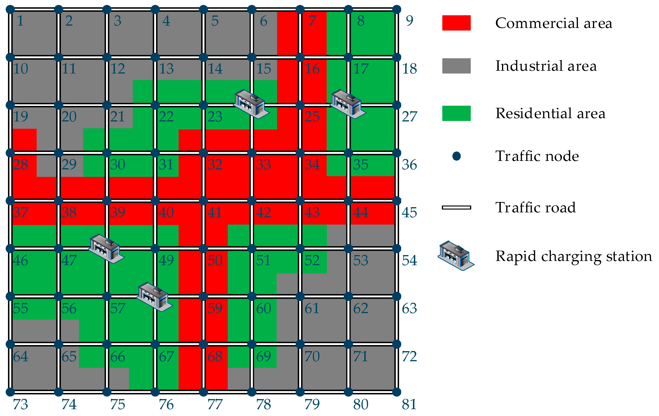
| Area Type | Residential Area | Industrial Area | Commercial Area |
|---|---|---|---|
| Land rental cost ($/m2) [40] | 330 | 109 | 1070 |
| Time cost ($/h) | 5.76 [49] | 5.25 | 3.82 |
| Feasible Solutions | Siting Results | Number of Chargers | Rank of Charging Stations |
|---|---|---|---|
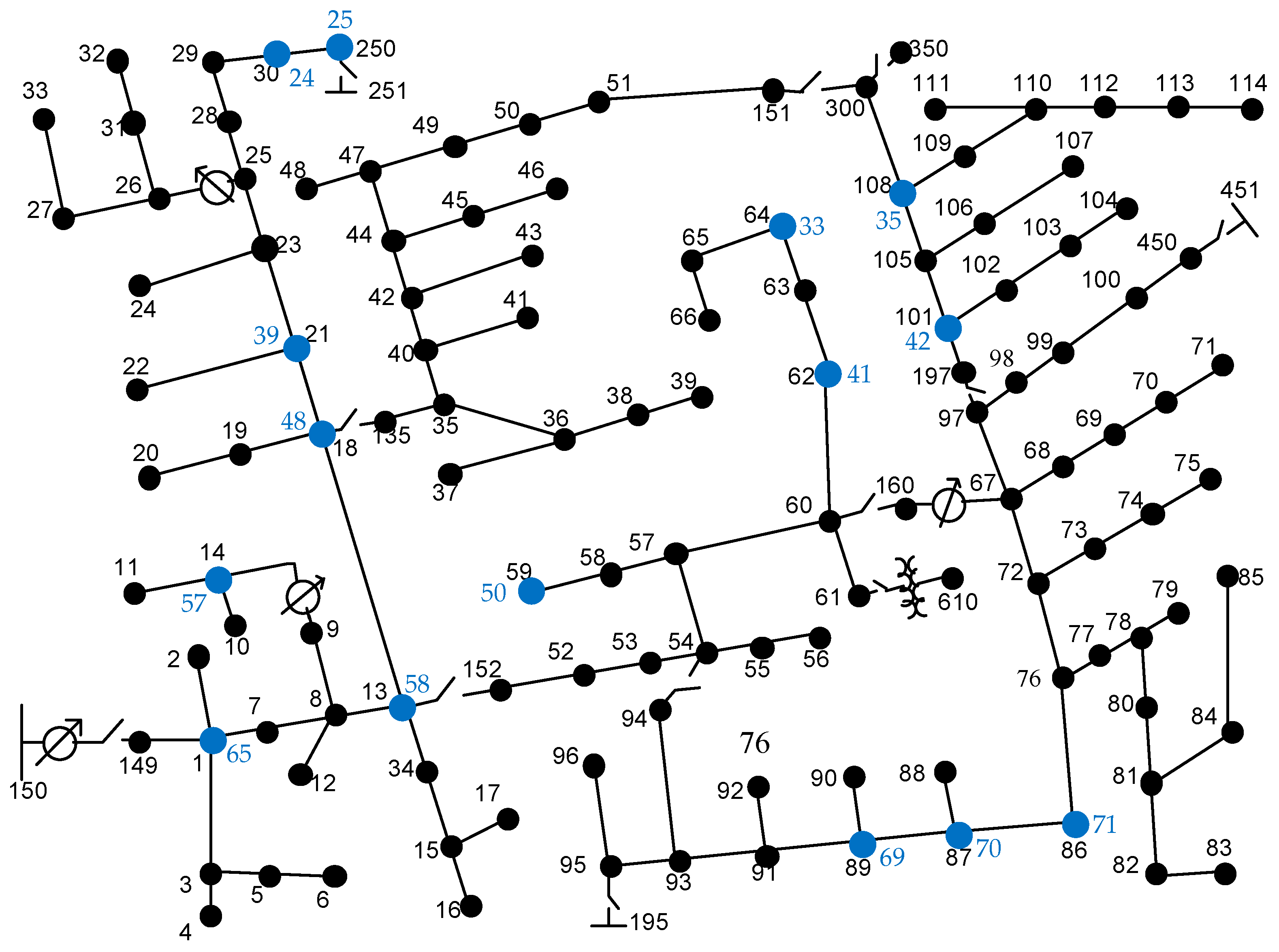
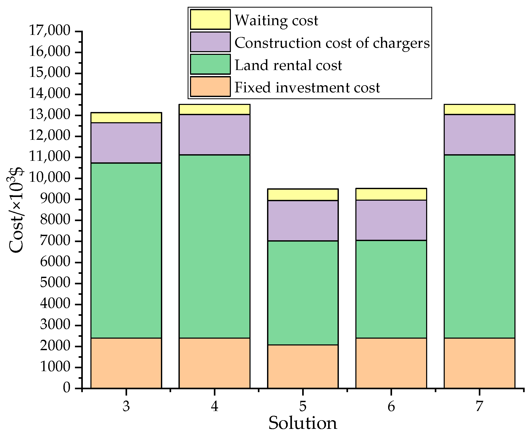
| 1 | 25, 33, 41, 57 | 29, 23, 24, 24 | 3, 3, 3, 3 |
| 2 | 25, 42, 41, 57 | 34, 18, 22, 26 | 2, 3, 3, 3 |
| 3 | 48, 25, 58, 70 | 36, 32, 24, 8 | 2, 2, 3, 4 |
| 4 | 48, 25, 58, 69 | 36, 32, 24, 8 | 2, 2, 3, 4 |
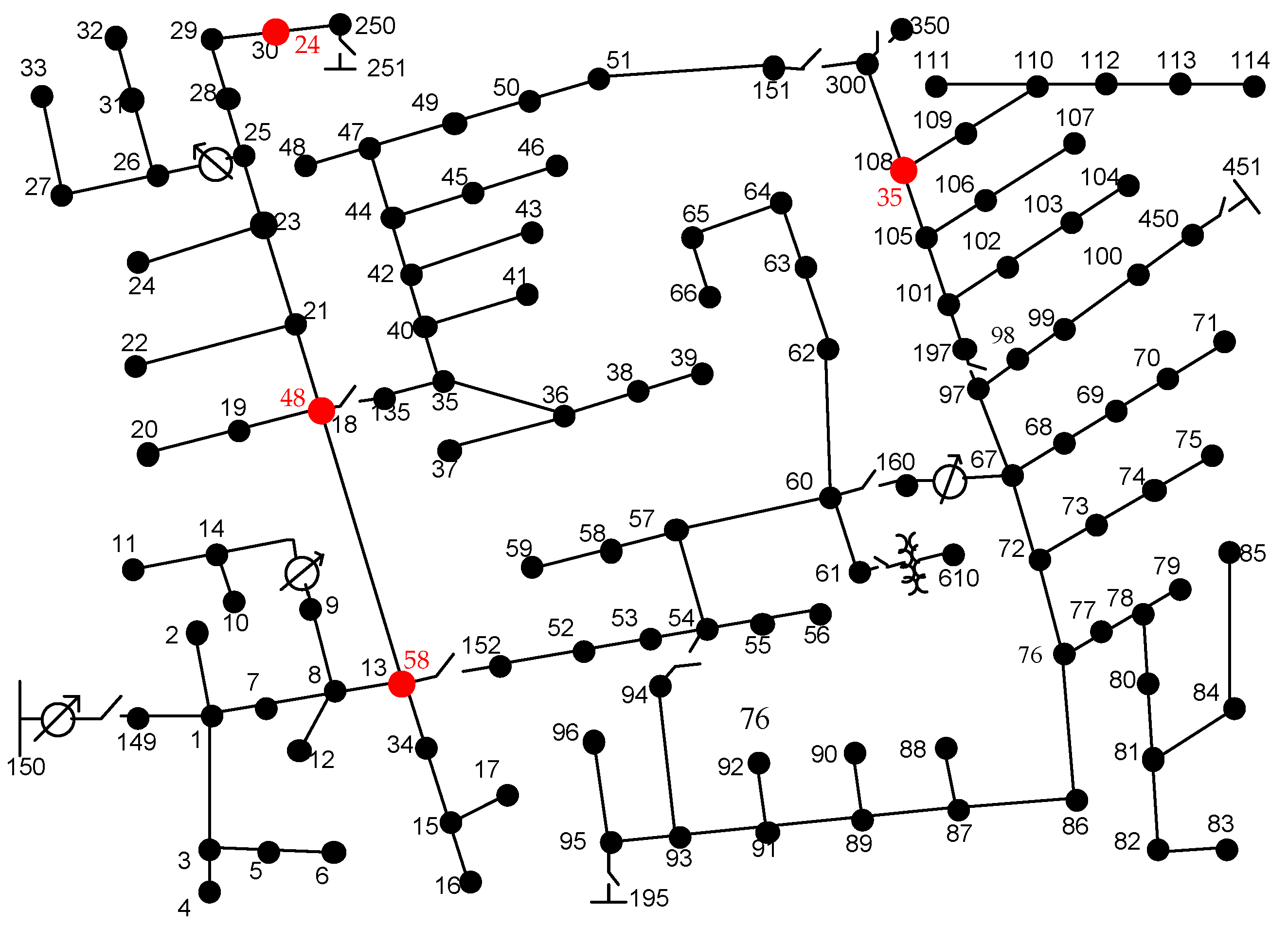
| 5 | 48, 24, 35, 58 | 39, 29, 13, 19 | 2, 3, 4, 3 |
| 6 | 48, 24, 71, 58 | 35, 35, 9, 21 | 2, 2, 4, 3 |
| 7 | 48, 25, 69, 58 | 38, 34, 8, 20 | 2, 2, 4, 3 |
| 8 | 41, 57, 35, 39 | 37, 32, 23, 8 | 2, 2, 3, 4 |
| 9 | 25, 50, 42, 65 | 38, 26, 13, 23 | 2, 3, 4, 3 |
© 2018 by the authors. Licensee MDPI, Basel, Switzerland. This article is an open access article distributed under the terms and conditions of the Creative Commons Attribution (CC BY) license (http://creativecommons.org/licenses/by/4.0/).
Share and Cite
Zang, H.; Fu, Y.; Chen, M.; Shen, H.; Miao, L.; Zhang, S.; Wei, Z.; Sun, G. Bi-Level Planning Model of Charging Stations Considering the Coupling Relationship between Charging Stations and Travel Route. Appl. Sci. 2018, 8, 1130. https://doi.org/10.3390/app8071130
Zang H, Fu Y, Chen M, Shen H, Miao L, Zhang S, Wei Z, Sun G. Bi-Level Planning Model of Charging Stations Considering the Coupling Relationship between Charging Stations and Travel Route. Applied Sciences. 2018; 8(7):1130. https://doi.org/10.3390/app8071130
Chicago/Turabian StyleZang, Haixiang, Yuting Fu, Ming Chen, Haiping Shen, Liheng Miao, Side Zhang, Zhinong Wei, and Guoqiang Sun. 2018. "Bi-Level Planning Model of Charging Stations Considering the Coupling Relationship between Charging Stations and Travel Route" Applied Sciences 8, no. 7: 1130. https://doi.org/10.3390/app8071130