Turning Gait Planning Method for Humanoid Robots

Abstract

The most important feature of this paper is to transform the complex motion of robot turning into a simple translational motion, thus simplifying the dynamic model. Compared with the method that generates a center of mass (COM) trajectory directly by the inverted pendulum model, this method is more precise. The non-inertial reference is introduced in the turning walk. This method can translate the turning walk into a straight-line walk when the inertial forces act on the robot. The dynamics of the robot model, called linear inverted pendulum (LIP), are changed and improved dynamics are derived to make them apply to the turning walk model. Then, we expend the new LIP model and control the zero moment point (ZMP) to guarantee the stability of the unstable parts of this model in order to generate a stable COM trajectory. We present simulation results for the improved LIP dynamics and verify the stability of the robot turning.

1. Introduction

The basic functionality required for humanoid robots is the ability to achieve various human movements. There are several existing methods for the planning and control of walking without revolving around the axis perpendicular to the horizontal plane [1,2,3,4,5]. The more challenging problem inherent to controlling a biped robot is maintaining its stability when it is moving. A widely used method for determining the stability of the robots is whether the zero moment point (ZMP) is in the supporting area [6,7]. In the trajectory planning method, the ZMP is seen as a linear inverted pendulum (LIP) which is a simplified model. The robot is regarded as a point, and the entire mass is concentrated at the center of the mass. Another trajectory planning method considers the humanoid robot as a seven-link model. The position of the ZMP can be calculated by the state of the COM of every link rod including the position, the velocity and the acceleration [8]. By comparing the ZMP trajectories, the trajectory with the highest stability margin is selected as the off-line trajectory. These methods have unique advantages and disadvantages. Recently, newer gait-planning methods [9,10,11,12,13] have been developed that do not rely on the ZMP and have indeed produced marked improvements in humanoid robot walking.

However, it is also very important for humanoid robots to be able to turn while walking at a high speed. For the robot to achieve various types of locomotion and efficiently complete any given task, it must be capable of turning while walking at a high speed. When the robot turns at a very low speed, the trajectory of the center of mass can be generated by the traditional LIP. However, the robot is likely to tip over during fast turns, but only if the trajectory is only generated by the LIP. Unlike straight-line walk (or “linear walk”), the so-called “turning walk” requires highly complex dynamical systems. During turning walk, the COM moves as it does during linear walk but while simultaneously performing circular motions, so in the world reference, the robot can not be seen as a particle. There are two choices that can be chosen to deal with the turning walk. One is to establish the humanoid robot whole body dynamics model in the world reference. The other is to translate the turning walk into the straight-line walk by choosing an appropriate non-inertial reference, and, in the non-inertial reference, the LIP model can also be used to generate the trajectory while the dynamics of the LIP are changed. There is an extended model of the LIP that is applied to the trajectory planning of the robot. The most popular model is the spring loaded inverted pendulum (SLIP) [14,15,16] which is used in robot running. In robot running, the LIP model causes big collisions to the ground, so in order to reduce the force that is generated by the collisions, the SLIP is proposed and has produced a good effect.

Previous researchers have indeed explored dynamic turning. The most famous example is the ASIMO robot, which can turn while walking and even while running. Soichiro Suzuki [17] achieved a quasi-passive turn walk by utilizing a mechanical oscillator. There has also been research into slip turns; Kanehiro presented a novel hierarchical controller for walking torque-controlled humanoid robots [18,19] which is capable of executing quick slip-turns on a HRP-4C on its toes. Koeda at al. achieved slip-turns in the HOAP-2 robot [20,21,22,23]. Their method minimizes the turning angle based on variations in friction across the floor. Despite these valuable contributions, there has been relatively little research on turning while the robot is walking.

Most research has applied straight-line walking models directly to the turning walks [24]. This method does not take into account the effect of the robot’s own rotation on the actual ZMP so in the lateral direction, the actual ZMP will be different form the planned ZMP. Due to the large model error, the robot will be easily unstable. So, the proposed method can reduce the model error to guarantee the stability of the robot. The main contribution of the paper is that our method takes into account the rotation factors in the turning process without increasing the complexity of the dynamics. So, the model is more accurate and the trajectory can be generated very fast.

The remainder of the paper is organized as follows. In Section 2, we analyze the scope of application of LIP and the limitations of the LIP during turning walk. Then, we introduce a non-inertial reference that can convert the turning walk to the straight-line walk. In Section 3, we establish the improved LIP model in the non-inertial reference and extend its dynamics. Then, we analyze the stable component and unstable component of the LIP and get the trajectory of the center of mass (COM) by ensuring boundedness of COM trajectories for a given reference ZMP trajectory. In Section 4, we give the trajectory planning of the foot and convert the COM trajectory under non-inertial system to the trajectory in a world coordinate system which can be used in the control of the robot based on the current state. In Section 5, results from the simulations and experiments are presented to verify the feasibility of the proposed method.

2. Non-Inertial Reference in Turning Walk

In the translational movement, the robot can be seen as a mass point because when it is treated as a rigid, the motion of the COM can represent the motion of the whole body. However, in the turning walk, there is not only translational movement but also rotation around the axis perpendicular to the horizontal plane. So, the motion of the COM cannot represent the motion of the whole robot which will make the robot fall down. In this paper, we introduce the non-inertial reference in which the motion of the turning walk is the straight-line walk.

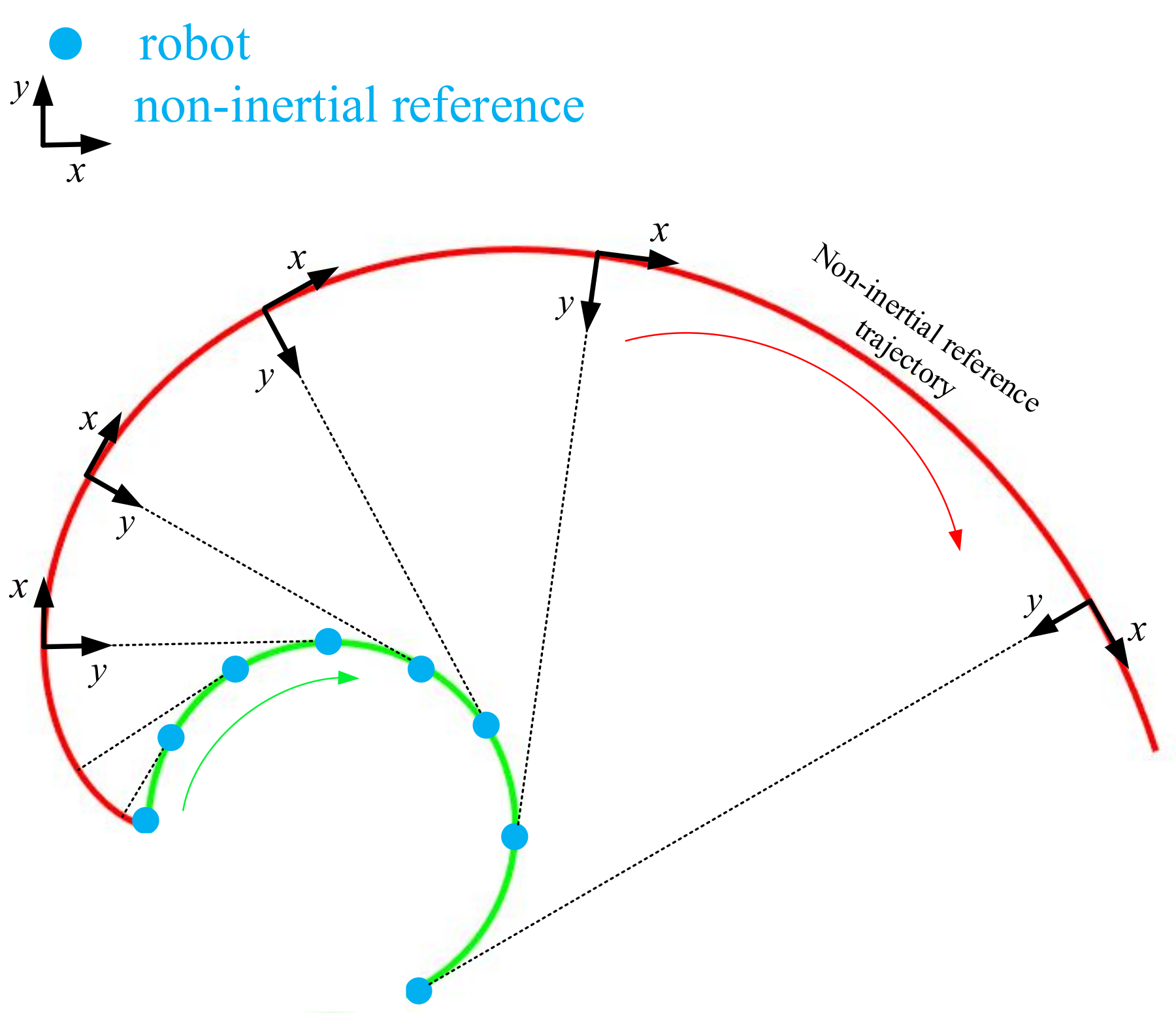
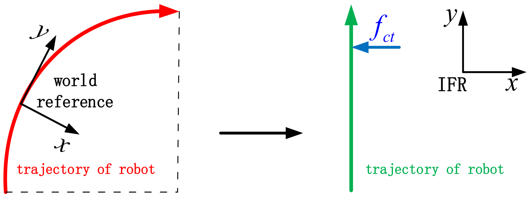
The motion of the non-inertial reference in the turning walking is shown in Figure 1, where the green curve represents the robot trajectory and the red curve represents the non-inertial reference. The non-inertial trajectory is defined as involute. The reference frame not only moves along the curve but also rotates which makes the Y-axis always point to the robot. In this paper, we call this the “involute reference frame” (IRF). In the IRF, the motion of the robot can be described similarly to straight-line walk.

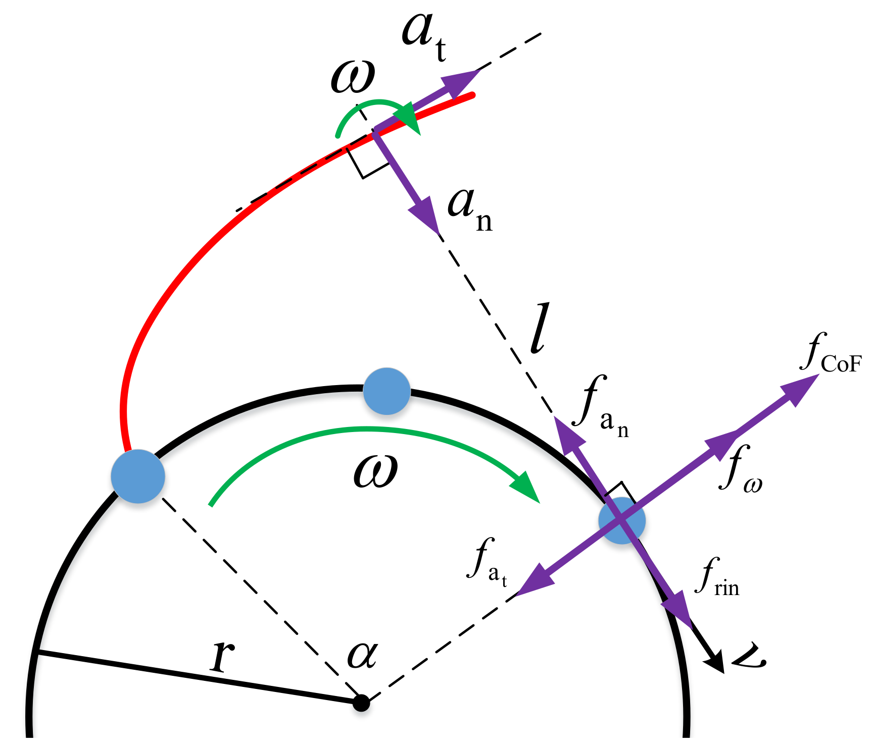
For the IRF, its motion has tangential acceleration, normal acceleration, and centripetal acceleration that rotates synchronously with circular motion. The motion of the object moving in the IRF is affected by inertial forces. The motion of the IRF and the inertial forces acting on the robot are shown in Figure 2. $a_t$ is the tangential acceleration; $a_n$ is the normal acceleration; and $\omega$ is the angular velocity. $f_{a_n}$ is generated due to normal acceleration, $f_{a_t}$ is generated due to tangential acceleration and $f_{rin}$ is generated due to centripetal acceleration. $f_{CoF}$ is the coriolis force. $f_{\omega }$ is the force generated due to the changing rate of angular velocity. All the inertial force expressions can be obtained as shown in Formula (1). l is the distance that the robot walks in the forward direction and is also the length between the origin of the IRF and the tangent point of the circle.

$$\left\{\begin{array}{c}{f}_{{\mathrm{a}}_{\mathrm{n}}}=m{\omega }^{2}r\hfill \\ f_{{\mathrm{a}}_{\mathrm{t}}}=m(\dot{\omega }l+\omega \dot{r})\hfill \\ f_{\mathrm{rin}}=m{\omega }^{2}r\hfill \\ f_{\mathrm{CoF}}=2m\omega v\hfill \\ f_{\omega }=m\dot{\omega }r.\hfill \end{array}\right.$$

(1)

where m is the mass of the object moving in the non-inertial frame, and r is the turning radius. The directions of the inertial centrifugal force ($f_{\mathrm{rin}}$) and normal force ($f_{{\mathrm{a}}_{\mathrm{n}}}$) are opposite, so the effect of the two forces cancels out. It is only necessary to calculate the $f_{\omega }$, $f_{\mathrm{rin}}$ and $f_{\mathrm{CoF}}$ in the IRF. Through the relationship between the physical quantities shown in Formula (2), we can simplify this force based on the involute properties in Formula (3).

$$l=\alpha r,v=\omega r,\dot{\alpha }=\omega$$

(2)

$$\left\{\begin{array}{c}{f}_{\mathrm{CoF}}=2m{\omega }^{2}r\hfill \\ f_{\omega }=m\dot{v}\alpha \hfill \\ f_{{\mathrm{a}}_{\mathrm{t}}}=m(\dot{v}\alpha +\frac{v^2}{r}).\hfill \end{array}\right.\left(3\right)$$

where v is the velocity in the forward direction related to the IRF and it is also the tangential velocity of circular motion related to the global reference. $\alpha$ is the angle that the robot turns. $f_{a_t}$ is a changing force which is determined by the acceleration and velocity of the object.

In Formula (4), through the the vector superposition of these inertial forces, $f_{\mathrm{sum}}$ is the resultant of inertial force applied to an object moving in the IRF, and its direction is the same as that of $f_{{\mathrm{a}}_{\mathrm{t}}}$

$$\begin{array}{c}{\mathbf{f}}_{\mathrm{sum}}={\mathbf{f}}_{\mathrm{CoF}}+{\mathbf{f}}_{{\mathrm{a}}_{\mathrm{t}}}+{\mathbf{f}}_{{\mathrm{a}}_{\mathrm{n}}}+{\mathbf{f}}_{\mathrm{rin}}+{\mathbf{f}}_{\omega }\\ f_{\mathrm{sum}}=m\left(\frac{v^2}{r}\right).\end{array}$$

(4)

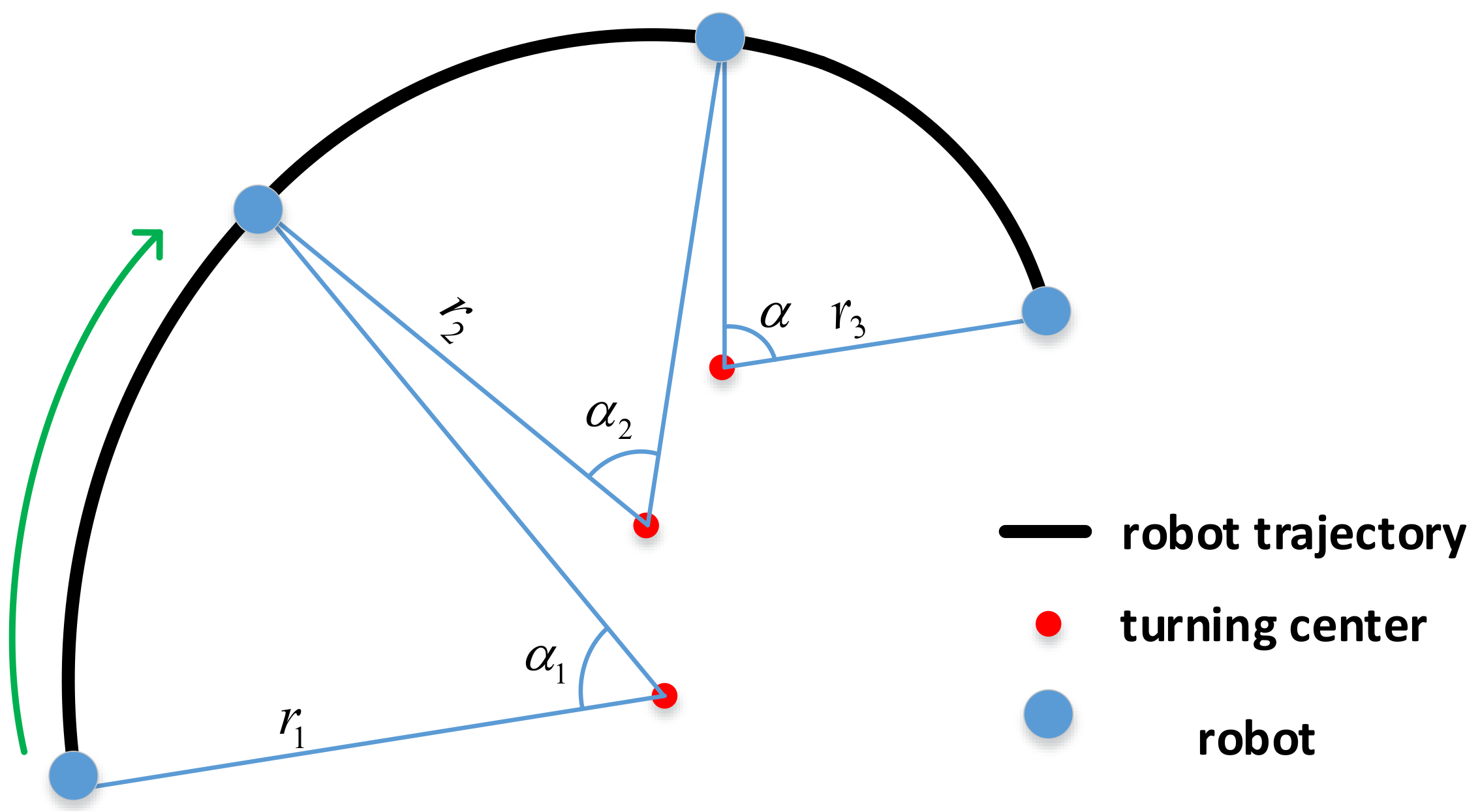
The discussion above centers around a scenario in which the turning radius is constant. During turning walk, however, the radius must change so that the robot can reach its target destination. Turning walk can be divided into several movements across a constant radius, where the expression of the resultant force does not change. As shown in Figure 3, if the radius is $r_1$, the force is $f_{\mathrm{sum}}^{\prime }=m\frac{v^2}{r_1}$. Similarly, $r_2$, $r_3$, and so on.

3. Turning Gait Planning in the Non-Inertial Reference (IRF)

3.1. Planning of the COM Trajectory

In order to make the description more intutive, we first define three directions related to the robot. The forward direction is called the y direction. The leftward and rightward direction is called the x direction. The vertical direction is called the z direction.

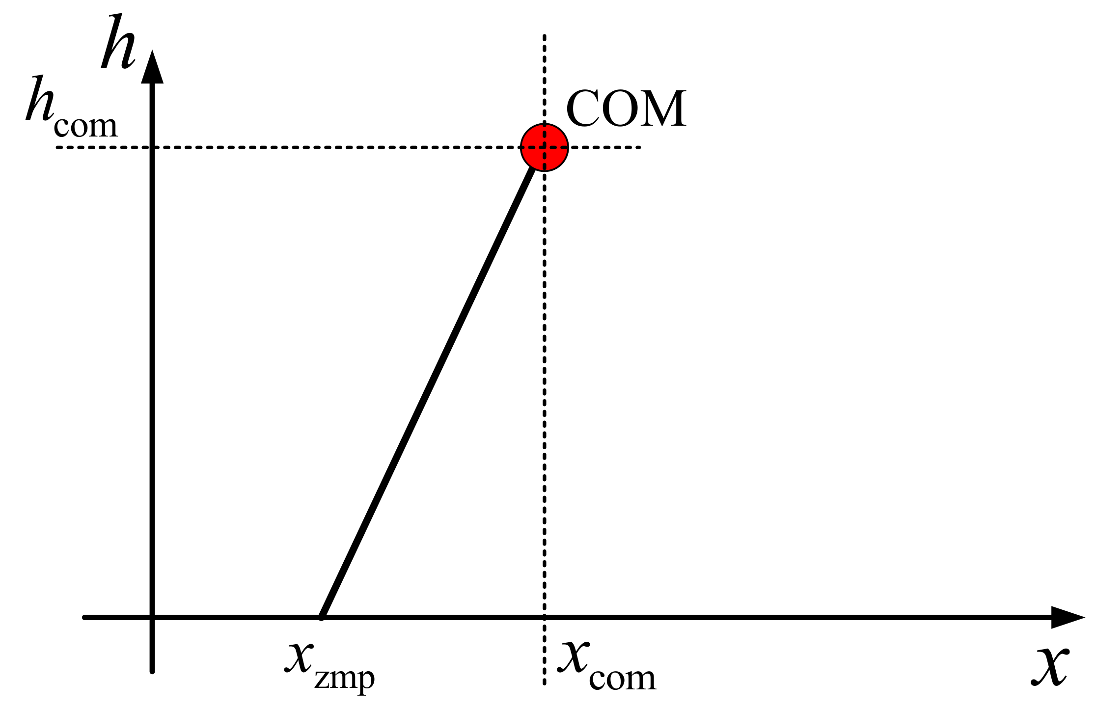
As the basic model of the robot walking, the LIP model simplifies the complex dynamic model of the robot. As is shown in Figure 4, the trajectory of the COM can represent the robot motion when the robot only moves in translation.

$${\ddot{x}}_{\mathrm{com}}={\omega }^2(x_{\mathrm{com}}-x_{\mathrm{zmp}}).$$

(5)

Here, $\omega =\sqrt{\frac{g}{h_{\mathrm{com}}}}$. $h_{\mathrm{com}}$ is the height of the COM. $x_{\mathrm{zmp}}$ is the position of the ZMP which can be planned ahead. $x_{\mathrm{com}}$ is the position of the COM. The input of the LIP model is the $x_{\mathrm{zmp}}$ and the output is the $x_{\mathrm{com}}$. This model is applicable when the robot does not rotate around the z-axis.

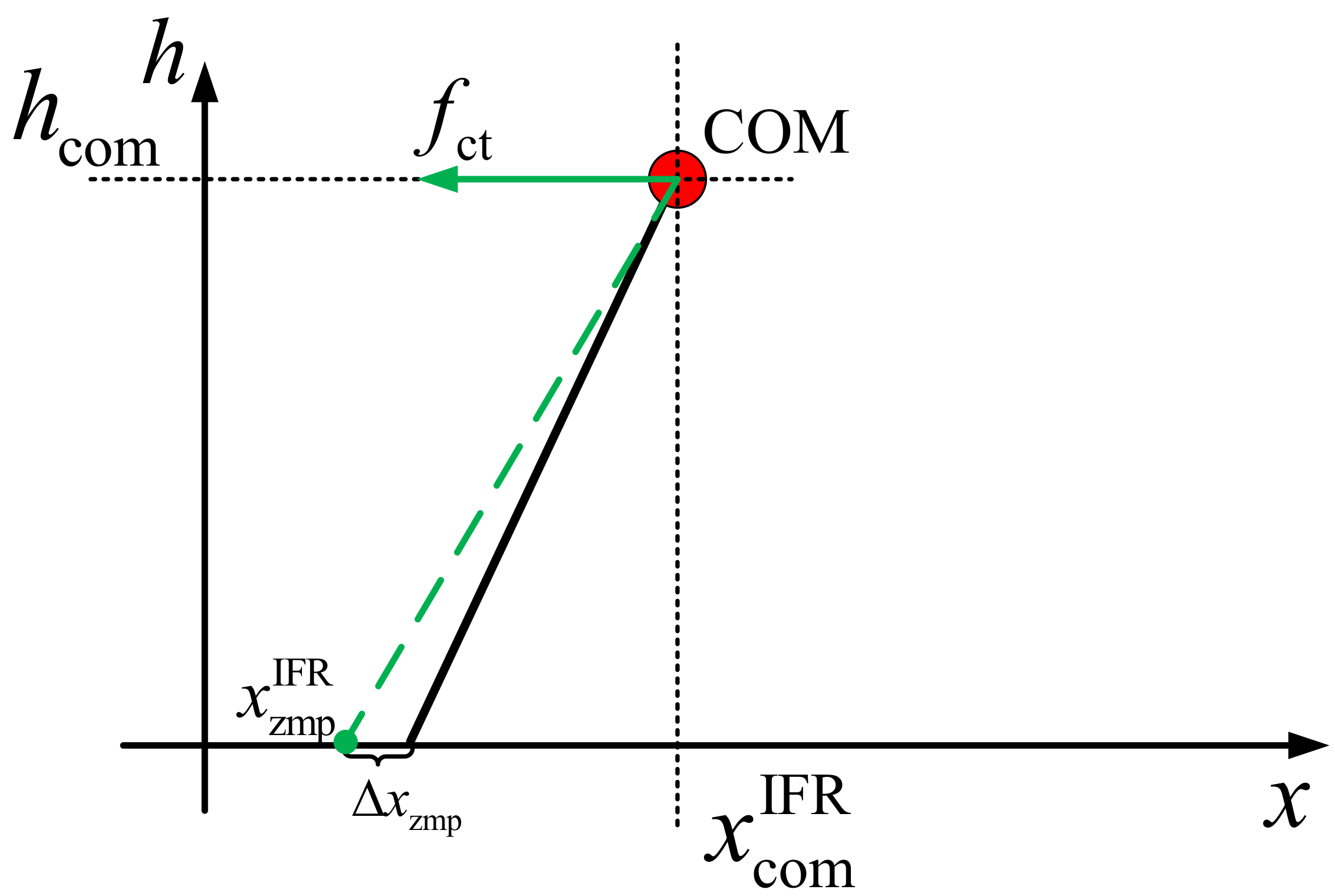
When compared with the straight-line walk, the system for the turning walk is more complex. For the turning walk, because of the existence of $f_{a_n}$, $f_{a_t}$, $f_{rin}$, and $f_{\omega }$. we must improve the traditional LIP model. As we can know from Section II, for the y direction in the IRF, the resultant of the inertial force is zero, so the traditional LIP is still applicable. However, for the x direction in the IRF, the resultant force is $f_{sum}$, so we can get the model of the turning walk from Figure 5. In this section, we call the $f_{\mathrm{sum}}$ force another name, $f_{ct}$, in order to simplify the subsequent derivation.

Because of force $f_{ct}$, the ZMP moves by a short distance. Based on this new model, we can then obtain the new dynamics.

$${\ddot{x}}_{\mathrm{com}}^{\mathrm{IRF}}={\omega }^2[x_{\mathrm{com}}^{\mathrm{IRF}}-(x_{\mathrm{zmp}}+\frac{\dot{y}{{}_{\mathrm{com}}^{\mathrm{IRF}}}^2}{{\omega }^2{r}_{\mathrm{com}}})],$$

(6)

where $r_c$ is the turn radius of the COM. $x_{\mathrm{zmp}}^{\mathrm{IRF}}$ is the ZMP position in the IRF, and $x_{\mathrm{com}}^{\mathrm{IRF}}$ is the COM position in the IRF. The $x_{\mathrm{zmp}}^{\mathrm{IRF}}$ position of the new ZMP has changed compared to that in the straight-line walk, as shown in Formula (7):

$$x_{\mathrm{zmp}}^{\mathrm{IRF}}=x_{\mathrm{zmp}}+\frac{\dot{y}{{}_{\mathrm{com}}^{\mathrm{IRF}}}^2}{{\omega }^2{r}_{\mathrm{com}}}.$$

(7)

So, the new LIP model can be expressed as follows:

$${\ddot{x}}_{\mathrm{com}}^{\mathrm{IRF}}={\omega }^2(x_{\mathrm{com}}^{\mathrm{IRF}}-x_{\mathrm{zmp}}^{\mathrm{IRF}}),$$

(8)

We can, therefore, treat turning walk as straight walk when we add the ZMP deviation: The new state space of the LIP system can then be expressed as $x^{\mathrm{IRF}}={[x_{\mathrm{com}}^{\mathrm{IRF}},{\dot{x}}_{\mathrm{com}}^{\mathrm{IRF}},x_{\mathrm{zmp}}^{\mathrm{IRF}}]}^T$. The input of the system is the velocity of the ZMP:

$${\dot{x}}^{\mathrm{IRF}}=\left[\begin{array}{ccc}0& 1& 0\\ {\omega }^2& 0& -{\omega }^2\\ 0& 0& 0\end{array}\right]x^{\mathrm{IRF}}+\left[\begin{array}{c}0\\ 0\\ 1\end{array}\right]{\dot{x}}_{\mathrm{zmp}}^{\mathrm{IRF}},$$

(9)

After doing the above simplification, turning walk can be converted into straight-line walk in the IRF when the straight-line walk is applied to a force ($f_{ct}$), as shown in Figure 6. Because the velocity of the COM in the y direction is not constant, the force $f_{ct}\left(\mathrm{t}\right)$ will also change all the time. According to Formula (7), we know that the $\Delta x_{\mathrm{zmp}}\left(\mathrm{t}\right)$ is also not constant:

$$f_{ct}\left(\mathrm{t}\right)=\mathrm{m}{\omega }^2(x_{\mathrm{zmp}}^{\mathrm{IRF}}\left(\mathrm{t}\right)-x_{\mathrm{zmp}}\left(\mathrm{t}\right))=\mathrm{m}{\omega }^2\Delta x_{\mathrm{zmp}}\left(t\right),$$

(10)

where m is the mass of the robot.

Through changes in the coordinates, this model can be divided into two components [7,25]. One is the stable mode and the other is the unstable mode, as is shown in Formula (11):

$$\begin{array}{c}{x}_{\mathrm{un}}=\frac{\omega x_{\mathrm{com}}^{\mathrm{IRF}}-{\dot{x}}_{\mathrm{com}}^{\mathrm{IRF}}}{\omega }\hfill \\ x_{\mathrm{st}}=\frac{\omega x_{\mathrm{com}}^{\mathrm{IRF}}+{\dot{x}}_{\mathrm{com}}^{\mathrm{IRF}}}{\omega }.\hfill \end{array}$$

(11)

We can then obtain an expression for $x_{\mathrm{un}}$, as shown in Formula (12). Formula (12) is a first-order differential equation, and its eigenvalue is an integrity, so this mode is a divergent system. The input of the subsystem is the position of the ZMP because the value of $\omega$ is constant:

$${\dot{x}}_{\mathrm{un}}\left(t\right)-\omega x_{\mathrm{un}}\left(t\right)=-\omega x_{\mathrm{zmp}}^{\mathrm{IRF}}\left(t\right).$$

(12)

In order to match the state space shown in Formula (9), the input of the system is the velocity of the ZMP. We can rewrite the expression in the Formula (13) when the radius of the COM is approximately constant:

$${\dot{x}}_{\mathrm{un}}\left(t\right)-\omega x_{\mathrm{un}}\left(t\right)=-\omega {\int }_0^t{\dot{x}}_{\mathrm{zmp}}^{\mathrm{IRF}}\left(t\right)dt\approx -\omega {\int }_0^t({\dot{x}}_{\mathrm{zmp}}\left(t\right)+\frac{2{\dot{y}}_{\mathrm{zmp}}^{\mathrm{IRF}}\left(t\right){\ddot{y}}_{\mathrm{zmp}}^{\mathrm{IRF}}\left(t\right)}{{\omega }^2{r}_{\mathrm{com}}})dt.$$

(13)

In the IRF, there is no inertial force in the forward direction y so the dynamics are the same as in the straight-line walk. We can calculate the ${\dot{y}}_{\mathrm{zmp}}^{\mathrm{IRF}}$ and ${\ddot{y}}_{\mathrm{zmp}}^{\mathrm{IRF}}$ based on the traditional LIP model ahead of time. Although $x_{\mathrm{un}}$ is divergent, we can find a ZMP trajectory whose initial condition satisfies $x_{\mathrm{un}}\left(t_{initial}\right)=\omega {\int }_{t_{initial}}^{\infty }{e}^{-\omega (t-t_{\mathrm{initial}})}{x}_{\mathrm{zmp}}^{\mathrm{IRF}}\left(t\right)dt$ to make the trajectory of the COM stable. According to the definition of $x_{\mathrm{un}}$, each control cycle $t_{initial}=k\delta$ can be used as the initial time for future trajectory planning. k can be $1,2\cdots n$, and $\delta$ is the control cycle. We can obtain the relationship between the state space and the velocity of ZMP to find this initial condition and the ZMP trajectory which is shown in Formula (14):

$$\frac{\omega x_{\mathrm{com}}^{\mathrm{IRF}}-{\dot{x}}_{\mathrm{com}}^{\mathrm{IRF}}}{\omega }=-\omega {\int }_{t_{\mathrm{initial}}}^{\infty }{e}^{-\omega (t-t_{\mathrm{initial}})}{\int }_{t_{\mathrm{initial}}}^{\infty }{\dot{x}}_{\mathrm{com}}^{\mathrm{IRF}}dtdt.$$

(14)

Here, we can obtain the relationship between the current state space of the COM, including the position and velocity and the future velocity of the ZMP. As is mentioned above, ZMP should be always in the supporting area to guarantee the stability of the robot, so the constraints of the velocity of ZMP are shown as Formula (15):

$$x_{\mathrm{zmp}}^{min}\left(t\right)\le x_{\mathrm{zmp}}^{\mathrm{IRF}}\left(t_{initial}\right)+{\int }_{t_{\mathrm{initial}}}^t{\dot{x}}_{\mathrm{zmp}}^{\mathrm{IRF}}\left(\tau \right)d\tau \le x_{\mathrm{zmp}}^{max}\left(t\right).$$

(15)

There are a lot of solutions to the COM trajectories that can satisfy the stable conditions for Formula (14). Through the optimal control theory, the input of the system is the velocity of ZMP, and we can reduce the value of the COM velocity deviating from the average speed, thus reducing the change in the COM velocity. We define the cost function (f) as the Formula (16):

$$f({\dot{x}}_{\mathrm{com}}^{\mathrm{IRF}}\left(t\right),t)={\int }_{t_{\mathrm{initial}}}^{\infty }{({\dot{x}}_{\mathrm{com}}^{\mathrm{IRF}}\left(t\right)-x_{\mathrm{com}}^{\mathrm{average}})}^{2}dt.$$

(16)

We discretize Formula (16) and obtain Formula (17):

$$f({\dot{x}}_{\mathrm{com}}^{\mathrm{IRF}}(k+j),k)=\sum _{j=0}^{j=N}{({\dot{x}}_{\mathrm{com}}^{\mathrm{IRF}}(k+j)-x_{\mathrm{com}}^{\mathrm{average}})}^2\delta ,$$

(17)

where N is the number of sampling points, and ${\dot{x}}_{\mathrm{com}}^{\mathrm{IRF}}((k+j)$ is the predicted COM velocity at the $j$th sampling point. The control variable is the ZMP velocity. We should thus derive the relationship between the velocities of the COM and the ZMP.

We can use the recursive method to predict the COM velocity after the velocities within the predicted time are known. These expressions are shown as Formula (18):

$$\begin{array}{c}{\dot{x}}_{\mathrm{com}}^{\mathrm{IRF}}(k+1)\hfill \\ ={\dot{x}}_{\mathrm{com}}^{\mathrm{IRF}}\left(k\right)+{\ddot{x}}_{\mathrm{com}}^{\mathrm{IRF}}\left(k\right)\delta ={\dot{x}}_{\mathrm{com}}^{\mathrm{IRF}}\left(k\right)+{\omega }^2(x_{\mathrm{com}}^{\mathrm{IRF}}\left(k\right)-x_{\mathrm{zmp}}^{\mathrm{IRF}}\left(k\right))\delta ,\hfill \\ {\dot{x}}_{\mathrm{com}}^{\mathrm{IRF}}(k+2)\hfill \\ ={\dot{x}}_{\mathrm{com}}^{\mathrm{IRF}}(k+1)+{\ddot{x}}_{\mathrm{com}}^{\mathrm{IRF}}(k+1)\delta \hfill \\ ={\dot{x}}_{\mathrm{com}}^{\mathrm{IRF}}(k+1)+{\omega }^2(x_{\mathrm{com}}^{\mathrm{IRF}}(k+1)-x_{\mathrm{zmp}}^{\mathrm{IRF}}\left(k\right)-{\dot{x}}_{\mathrm{zmp}}^{\mathrm{IRF}}\left(k\right)\delta )\delta ,\hfill \\ ⋮\hfill \\ {\dot{x}}_{\mathrm{com}}^{\mathrm{IRF}}(k+N)\hfill \\ ={\dot{x}}_{\mathrm{com}}^{\mathrm{IRF}}(k+N-1)+{\ddot{x}}_{\mathrm{com}}^{\mathrm{IRF}}(k+N-1)\delta \hfill \\ =\stackrel{·}{{\dot{x}}_{\mathrm{com}}^{\mathrm{IRF}}(k+N-1)}+{\omega }^2(x_{\mathrm{com}}^{\mathrm{IRF}}(k+N-1)-x_{\mathrm{zmp}}^{\mathrm{IRF}}\left(k\right)\hfill \\ -\stackrel{·}{{\dot{x}}_{\mathrm{zmp}}^{\mathrm{IRF}}\left(k\right)\delta -\cdots -{\dot{x}}_{\mathrm{zmp}}^{\mathrm{IRF}}(k+N-2)\delta })\delta .\hfill \end{array}$$

(18)

We therefore have the cost function, the stability constraint, and the ZMP constraint. We can obtain the ZMP velocity as the input for the new LIP model. We can, therefore, plan the ZMP and COM trajectories.

3.2. Foot Position and Allowable ZMP Region Planning

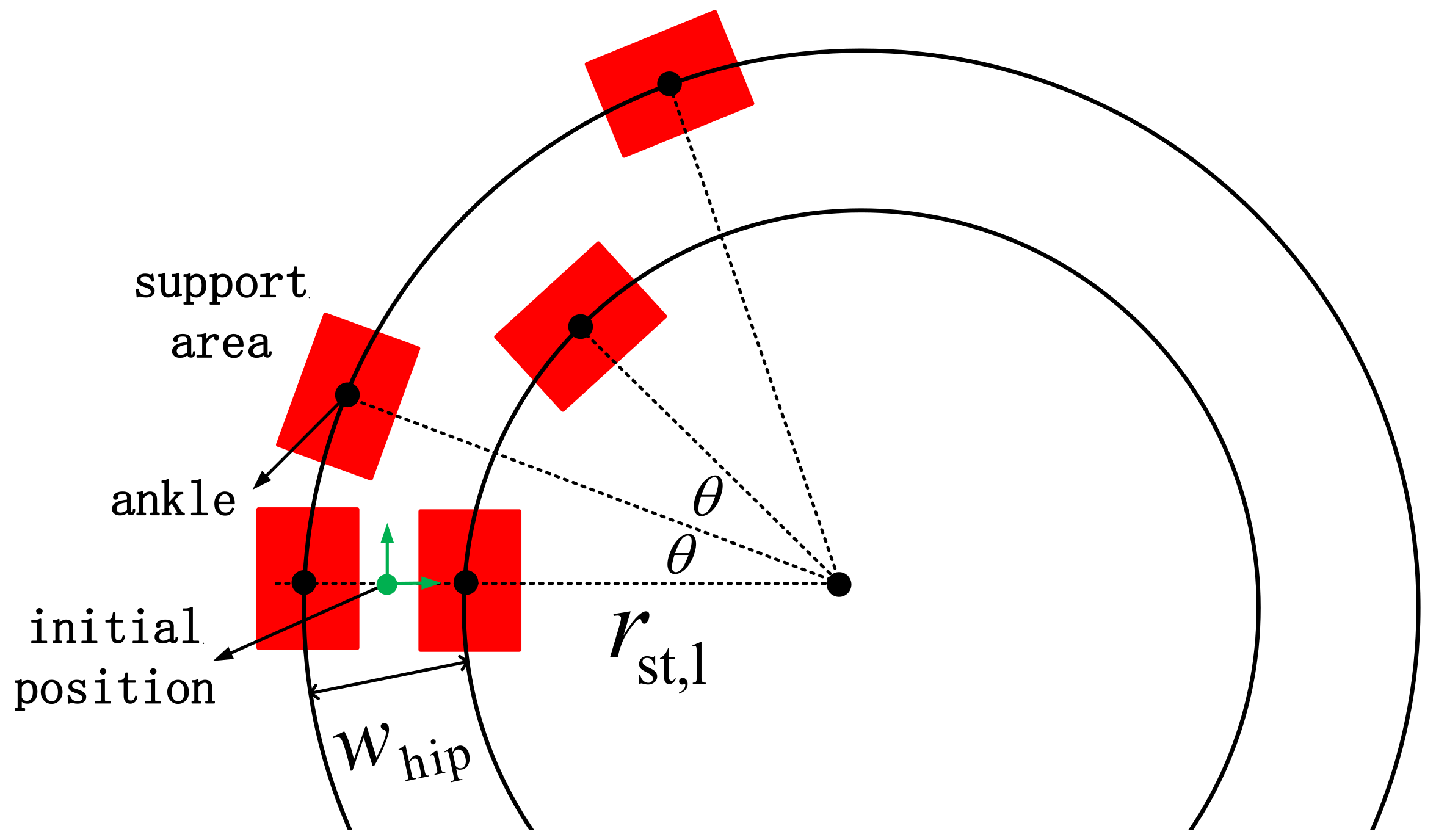
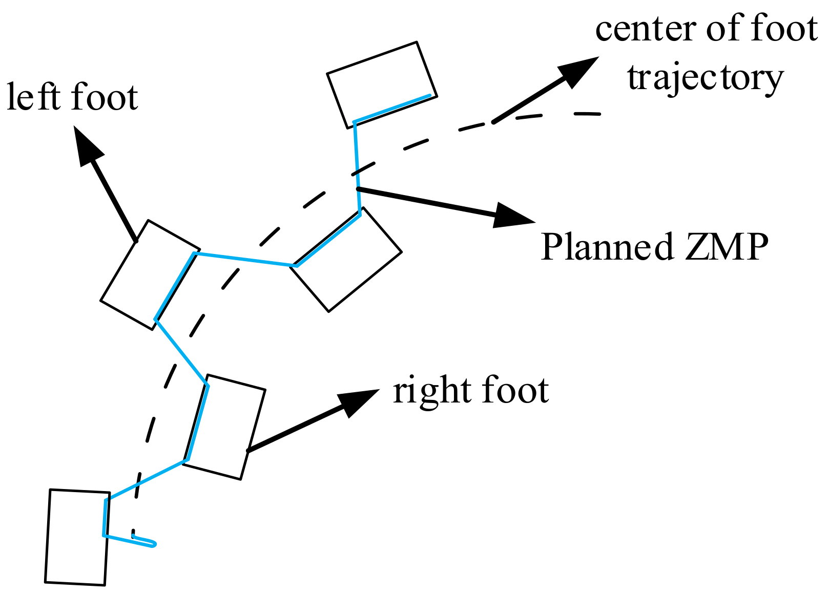
The foot position determines the area supporting the robot, so it must be determined first. For the turning walk, we use a circular curve interpolation to generate the foot trajectory, which is shown in Figure 7. In the single support period, the foot position of the swinging leg will follow the curve of the circle.

At this stage, we know the foot step, the walking cycle period, and the turning angle. In turning walk, the foot steps of the two legs are not the same. Therefore, we must first calculate the right foot radius ($r_{\mathrm{st},\mathrm{r}}$). The foot step is approximately equal to the arc length.

The radius of the left foot should be calculated as shown in Formula (19) in order to calculate the right foot radius:

$$r_{\mathrm{st},\mathrm{l}}=l_{\mathrm{st},\mathrm{l}}/\theta .$$

(19)

Suppose now that the robot turns right while walking. Here, $l_{\mathrm{st},\mathrm{l}}$ is the right foot step, and $\theta$ is the turning angle. The right foot radius is $r_{\mathrm{st},\mathrm{r}}=r_{\mathrm{st},\mathrm{l}}+w_{\mathrm{hip}}$. We can also obtain the right foot step as $l_{\mathrm{st},\mathrm{r}}=\theta (r_{\mathrm{st},\mathrm{l}}+w_{\mathrm{hip}})$, and $w_{\mathrm{hip}}$ is the distance between two feet. The foot trajectory is then generated by spline interpolation. The foot position can be calculated when the turning angle ($\theta \left(t\right)$) is known. The turning angle ($\theta \left(t\right)$) is obtained by cubic spline interpolation. This can guarantee that the foot speed at the beginning and end of the single support period is zero.

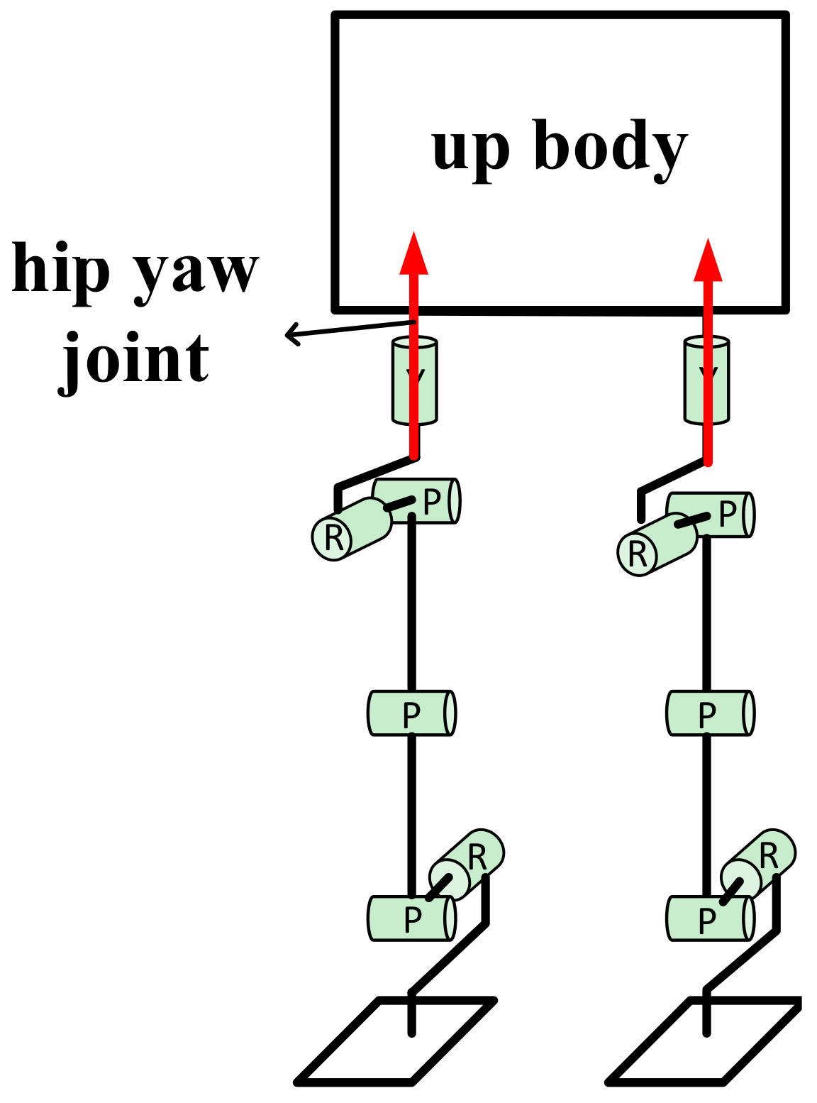
In straight-line walking, the foot coordinate only has translation related to the hip coordinate, so the hip yaw joint does not turn, but in turning walk, besides the translation, the foot coordinate also has rotation related to the hip coordinate, so the hip yaw joint will play a role in coordinate rotation shown in Figure 8.

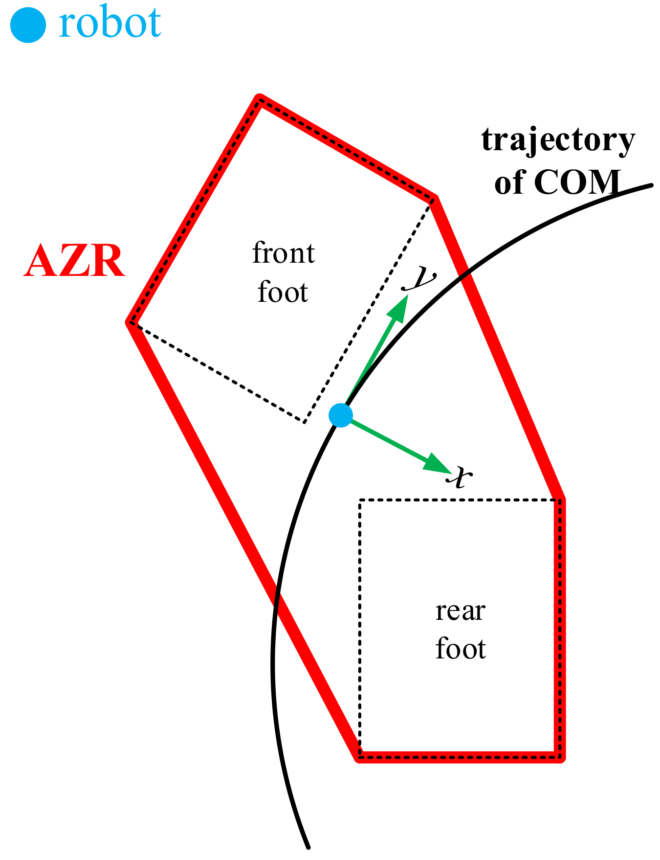
After the foot positions have been determined, the next step is planning the allowable ZMP region (AZR). This is a prerequisite for planning the ZMP trajectory. The AZR is the polygon that is surrounded by the supporting feet. However, for turning walk, the front foot direction differs from that of the rear foot. Therefore, in the double support period, the AZR is as shown in Figure 9.

The directions of the x and y coordinates are the same as those in the IRF. We suppose that the robot is at the position shown in Figure 9, and the position of AZR at the world coordinate reference is also known. So, we should express the AZR in the IRF. After we have determined the $\alpha$ and the position of $y_{\mathrm{com}}^{\mathrm{IRF}}$, we can easily obtain the expression of the AZR in the IRF through the positive kinematics.

4. Transformation from the IRF to the World Coordinate Reference

For the humanoid robot walk, what we need is the trajectory in the world coordinate reference so we need to convert the trajectory in the IRF into the trajectory under the world coordinate reference.

In the turning walk, the forward direction of the COM is always the tangential direction of the COM circle, so the COM direction is always changing. Once we have planned the foot position and the allowable ZMP region (AZR) in the world reference, we need to express them in the world coordinate reference. In the IRF, the distance passed through in the forward direction is the arc length of the turning walk in the world coordinate reference. First, we know that the radius of the COM differs from the radius of the foot. The radius of the average COM trajectory ($r_{\mathrm{c}}$) is in the range between the radii of the two feet. We can then obtain $r_{\mathrm{c}}$ from Formula (20). $w_{\mathrm{hip}}$ is the width of the robot hip:

$$r_{\mathrm{c}}=r+w_{\mathrm{hip}}/2.$$

(20)

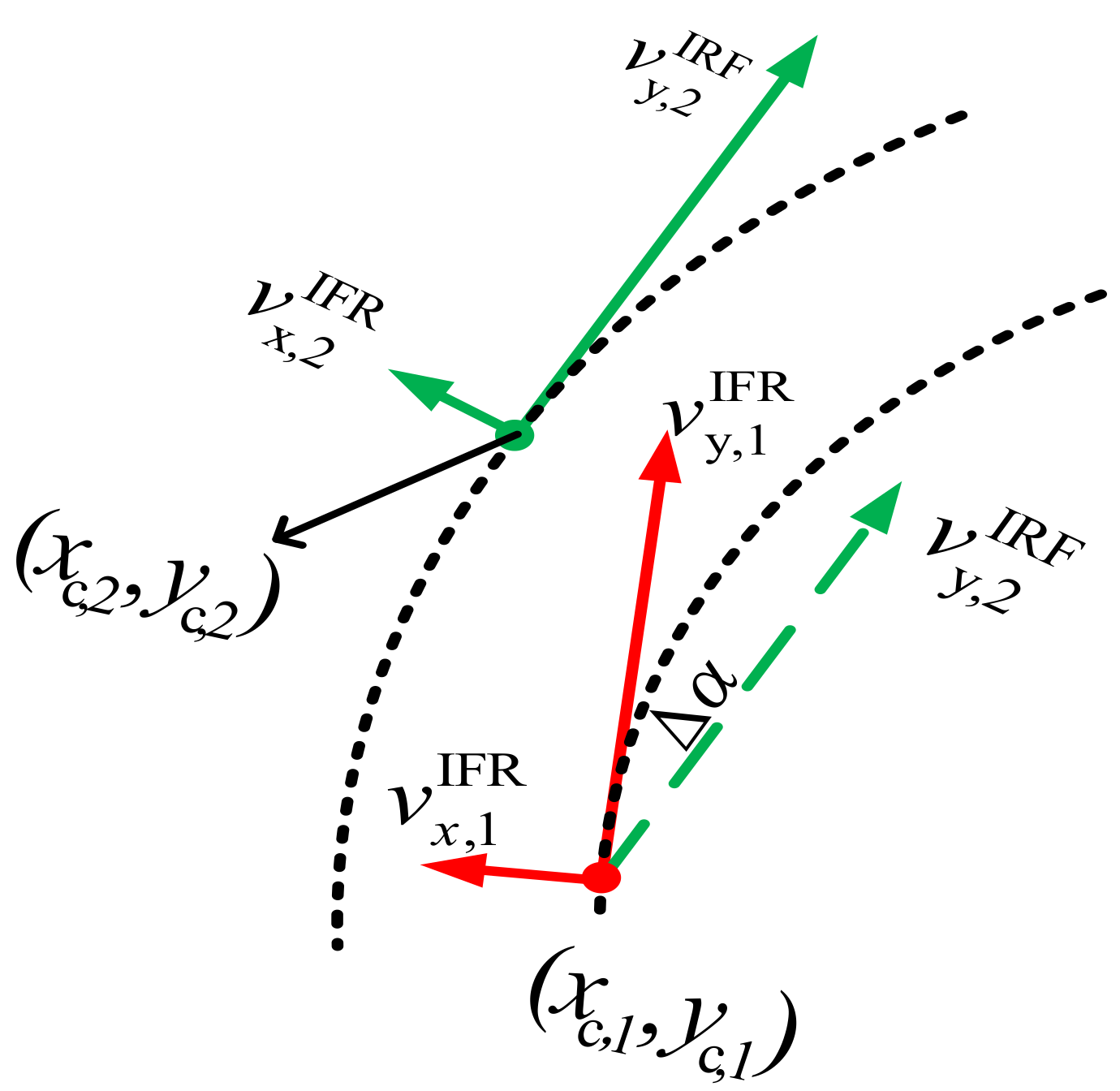
In one control cycle, the change in the angle of the COM direction ($\Delta \alpha$) can also be calculated as shown in Figure 10.

$$\Delta \alpha =\frac{y_{\mathrm{c},1}+v_{\mathrm{y},1}·\delta }{r_{\mathrm{c}}+x_{\mathrm{c},1}+v_{\mathrm{x},1}·\delta }-\frac{y_{\mathrm{c},1}}{r_{\mathrm{c}}+x_{\mathrm{c},1}},$$

(21)

where, $v_{x,1}^{IRF}$, $v_{y,1}^{IRF}$ are the velocities of the COM in the IRF at the current moment. $x_{\mathrm{c},1}$, $y_{\mathrm{c},1}$ is the position of the COM in the world coordinate reference at the current moment. $v_{x,2}^{IRF}$, $v_{y,2}^{IRF}$, $x_{\mathrm{c},2}$ and $y_{\mathrm{c},2}$ have the same meaning in the next control period. $\delta$ is the control cycle which depends on the controller’s operating speed. However, we can establish the relationship between the position in the world coordinate reference and the velocities in the IRF. The expression is shown in Formula (22):

$$\left[\begin{array}{c}{x}_{\mathrm{c},2}\\ y_{c,2}\end{array}\right]=\left[\begin{array}{c}{x}_{\mathrm{c},1}\\ y_{c,1}\end{array}\right]+\delta \left[\begin{array}{cc}cos\left(\alpha \right)& sin\left(\alpha \right)\\ -sin\left(\alpha \right)& cos\left(\alpha \right)\end{array}\right]\left[\begin{array}{c}{v}_{{}_{\mathrm{x},1}}^{\mathrm{IRF}}\\ v_{\mathrm{y},1}^{\mathrm{IRF}}\end{array}\right],$$

(22)

where

$$\alpha =\sum \Delta {\alpha }_i.$$

Turning Walk Planning Method

We can now provide an outline of the turning walk algorithm. First, we require the input data, including the foot steps and the turning angle. This information is then used to calculate the turning radius, the trajectory of the foot. and the AZR over the entire time span. What we need to know is the position and velocity of the COM and the ZMP position. In the initialization stage, these values are determined by hand, while future values are calculated by the model of the new LIP model.

The general $k-\mathrm{th}$ iteration proceeds as follows:

• Use the new cost function with stability and ZMP constraints to compute the ZMP velocity based on the new LIP model in the preceding section;
• Based on the planned ZMP velocity, we then obtain the ZMP position and can also get the position and velocity of COM in the IRF;
• Compute $\Delta \alpha$ based on the COM position and velocity;
• Based on $\Delta \alpha$, we can calculate the COM velocity and the ZMP position in the world coordinate reference. This is the turning walk data. We then return to the first step.

5. Simulations and Experiments

We now present some simulations of the BHR-6 humanoid robot of Beijing Institute of Technology to illustrate the performance of the turning gait planning method. The robot parameters are shown in

Table 1. Parameters of robot BHR-6.

Parameters	Value
Degrees of freedom	23
Weight	50.0 kg
Height	1.65 m
Foot length	24 cm
Foot width	14 cm
Hip width	15 cm
Contact type	Point contact

. We also present some comparisons between two different walking speeds. Through comparing different walking speeds, we can determine the function of the proposed gait planning method.

The planned ZMP as-obtained by the cost function (f) is shown in Figure 11. We set the walking step to $T_{\mathrm{step}}=1.2\mathrm{s}$ and sampling cycle to $T_{\mathrm{sample}}=0.004$ s. The walking step was $D_{\mathrm{step}}=0.33$ m, and the turning radius was $r_c=1.06$ m; these are the planning results in the global reference frame. The ZMP was in the boundary of the supporting area and continued moving forward whether in the double supporting period or single supporting period. This planning result is similar to that of linear walking.

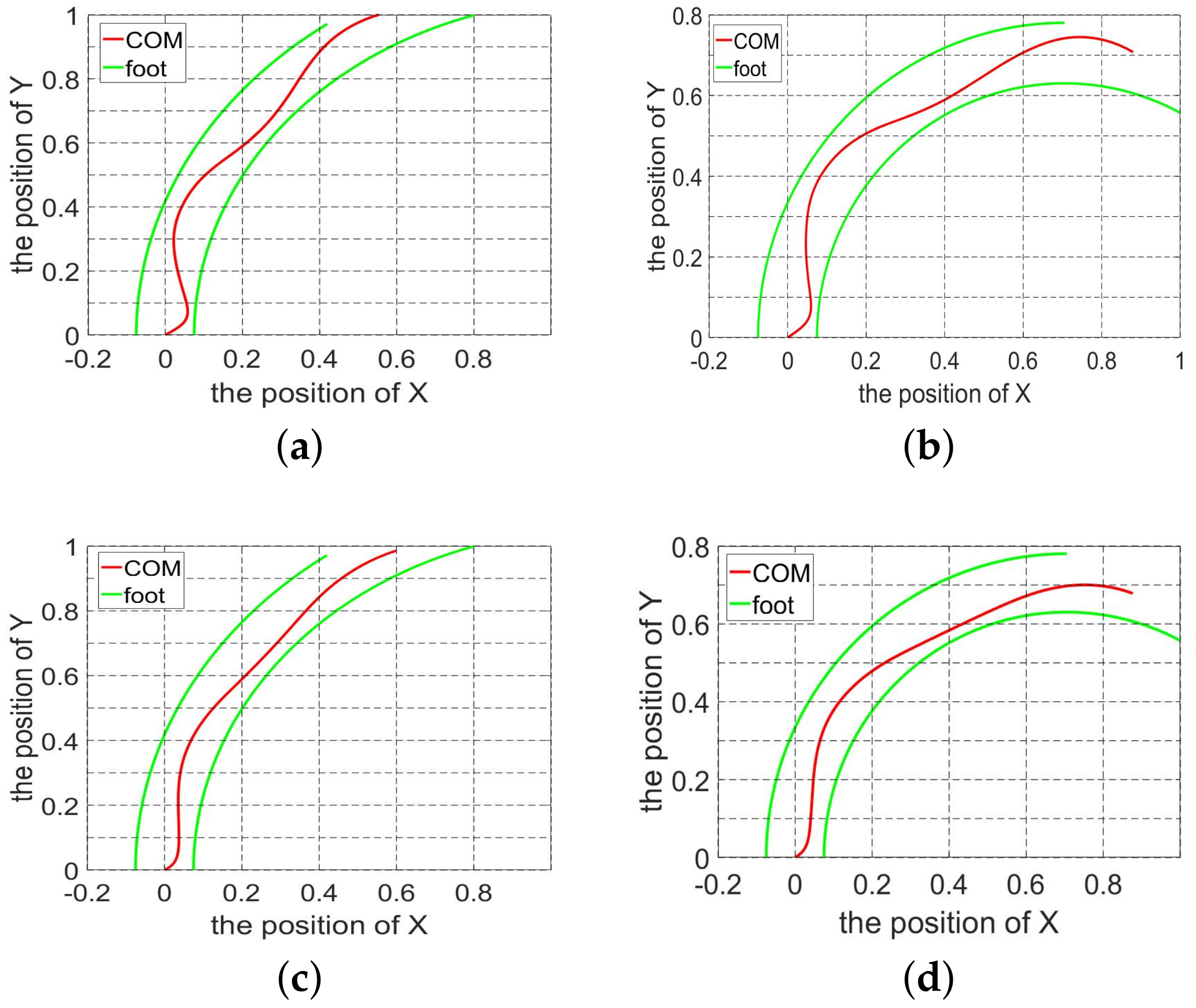
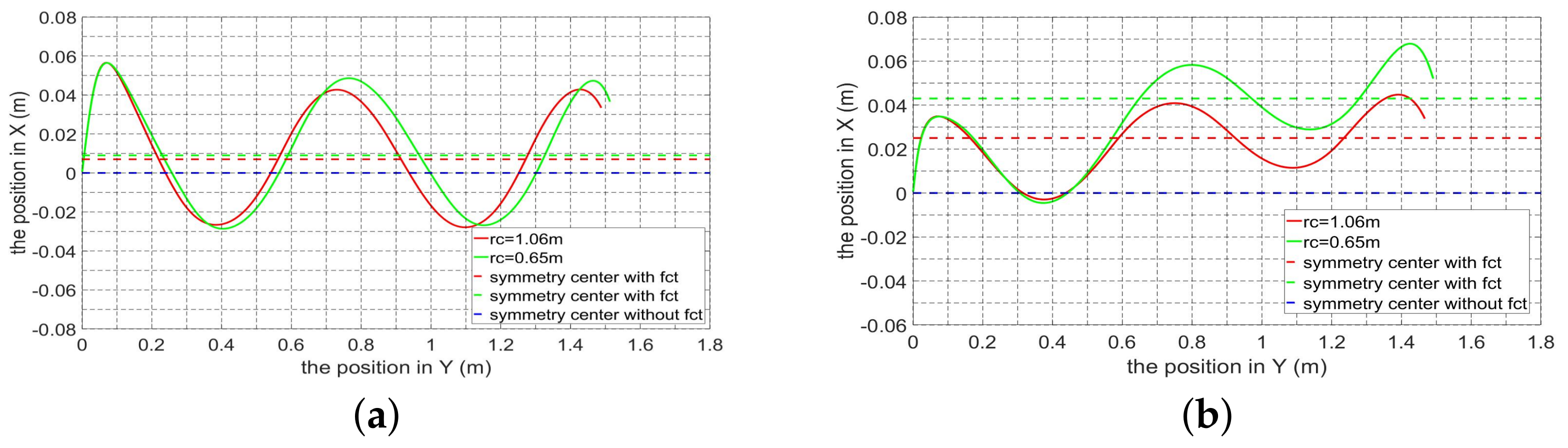
Once the ZMP trajectory was planned, the new trajectory was generated based on the new LIP model expressed in Formula (6). The formula is easy to be discretized. We simulated two walking speed trajectories with different radii and walking speeds to test the practicability of this method. As shown in Figure 12, the trajectory was generated as the robot turned to the right. As opposed to straight-line walk, turning walk creates a trajectory offset to the direction in which the robot is moving. When the robot turns right, the trajectory of COM will shift to the right and for left turns, it will shift to the left. As shown in Figure 13, the faster the robot moves, the more the trajectory is offset. The foot width of our BHR-6 was 14 cm but when the robot walking speed was 2 km per hour, the offset achieved $4.5$ cm with the radius $r_{\mathrm{c}}=0.67$ m. When the robot walks as slowly $1\mathrm{km}/\mathrm{h}$, the offset fell to $0.8$ cm with the same turn radius. For the same walking speed, the offsets caused by different radii were also different. For the walking speed $2\mathrm{km}/\mathrm{h}$ per hour, the offset was $2.5$ cm with the radius $r_{\mathrm{c}}=1.06$ m. When the robot walks slowly, the centroid shift caused by centripetal force can be neglected and the trajectory can be planned in the same manner as for straight-line walking.

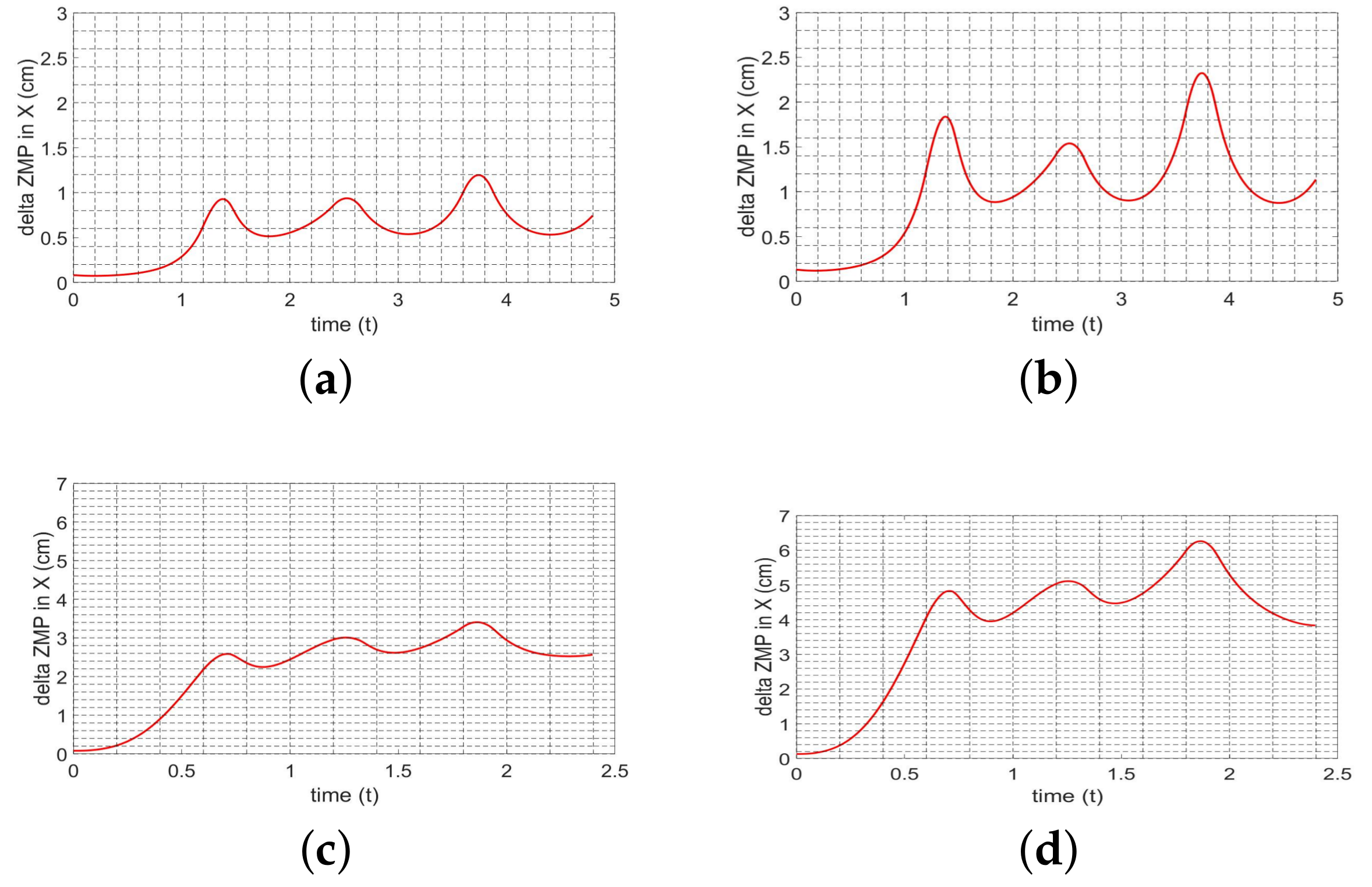
We reached the results shown in Figure 14 by calculating the $\Delta zmp$. Thus we can see the influence of robot rotation on the robot’s ZMP position. Both walking speed and turning radius had significant impacts on the offset of the ZMP. A decrease in the radius and increase in walking speed caused $\Delta zmp$ to increase. As shown in Figure 14d, when the radius was $0.67$ m and the walking speed was 2 km per hour, the greatest offset of ZMP was $6.2$ cm; this offset markedly affects the planning of the reference ZMP trajectory.

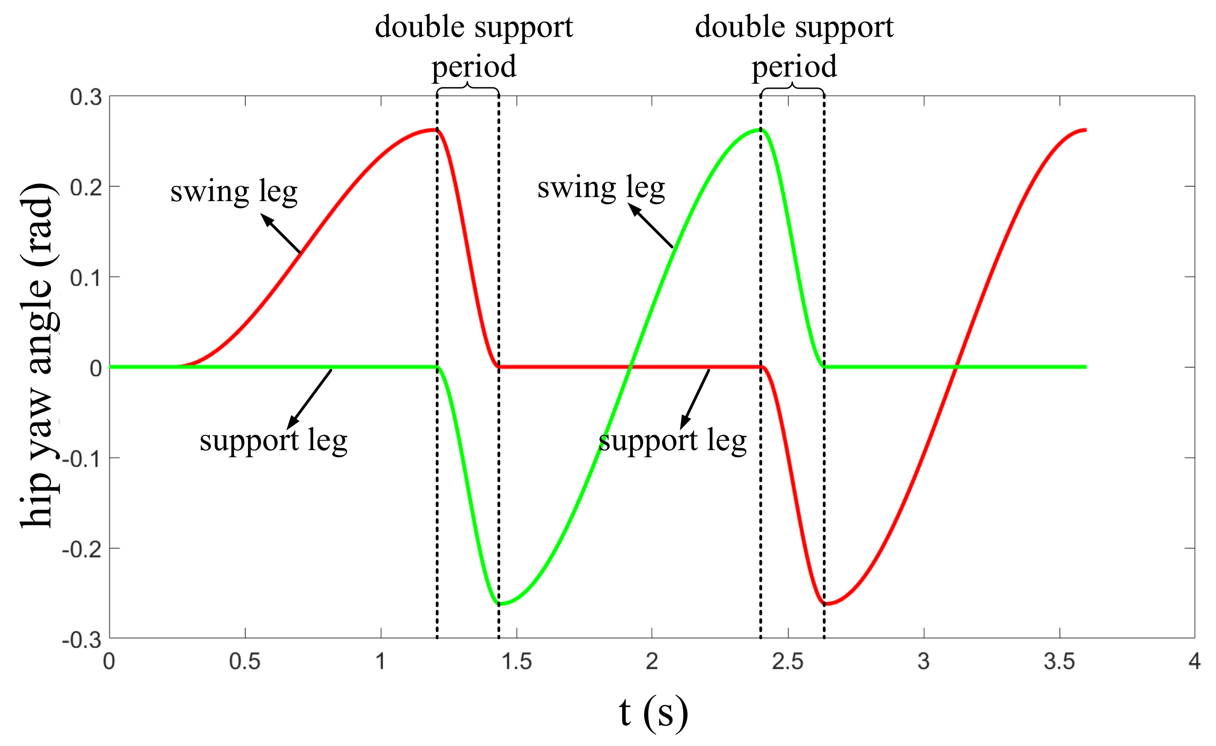
As opposed to straight-line walk, during turning walk, the hip yaw joints underwent major rotation at the angle shown in Figure 15. During a single support period, the supporting leg does not turn, and only the swinging leg turns. This means that the body does not turn. During a double support period, both hip yaw joints turn, and the body turns through an angle. Because the support area in the double support period is much larger than that in the single support period, the robot is less likely to slide on the ground when it turns fast. These phenomena correspond with the foot position planning results.

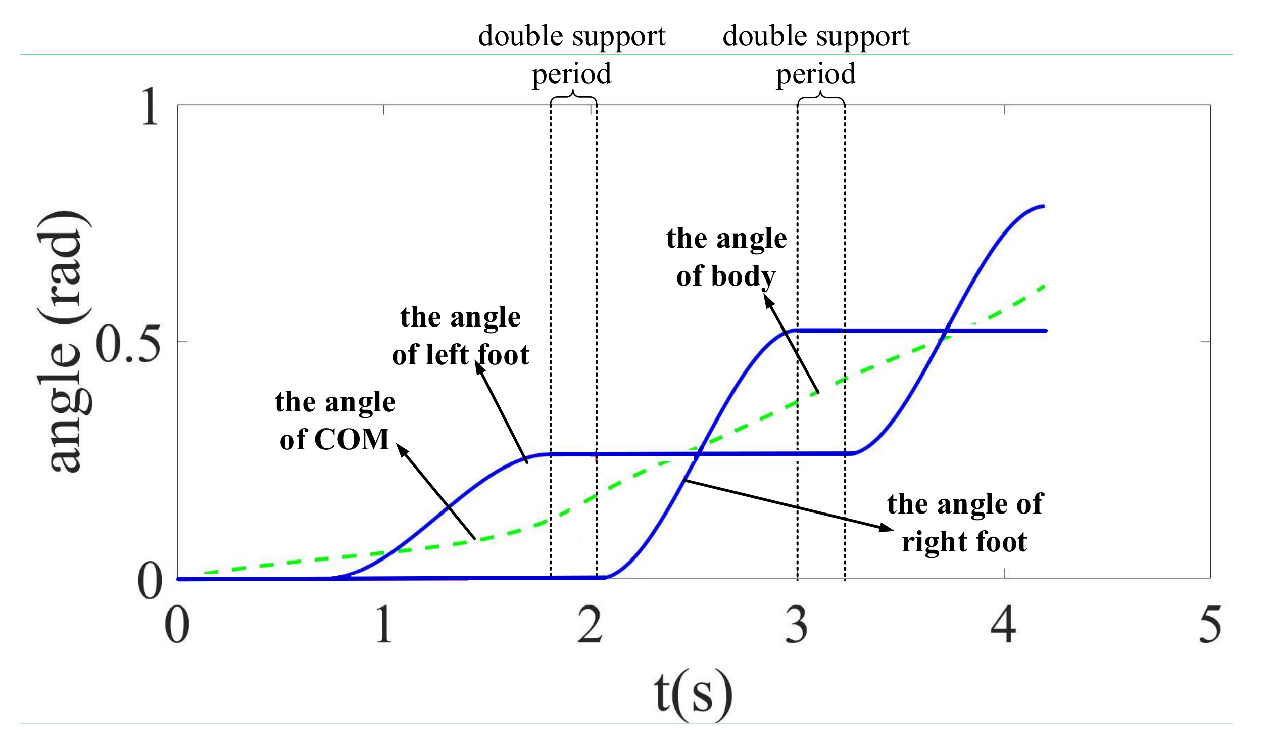
There are a few angles that must be defined properly for the purpose of turning walk. In Figure 16, the green line marks the COM angle (tangent direction of the turning motion) which equals the value of the upbody angle. It was obtained based on Formula (21) and Formula (22). The blue line is the foot angle, and the foot angle is planned before plotting the COM trajectory. In the single support period, the foot of the swing leg turns while the support leg maintains its previous state and in the double support period, the foot maintains its previous state. All these angles increase at the same average speed in one walk cycle so that at the end of every walk cycle, the direction of the feet and upbody is the same.

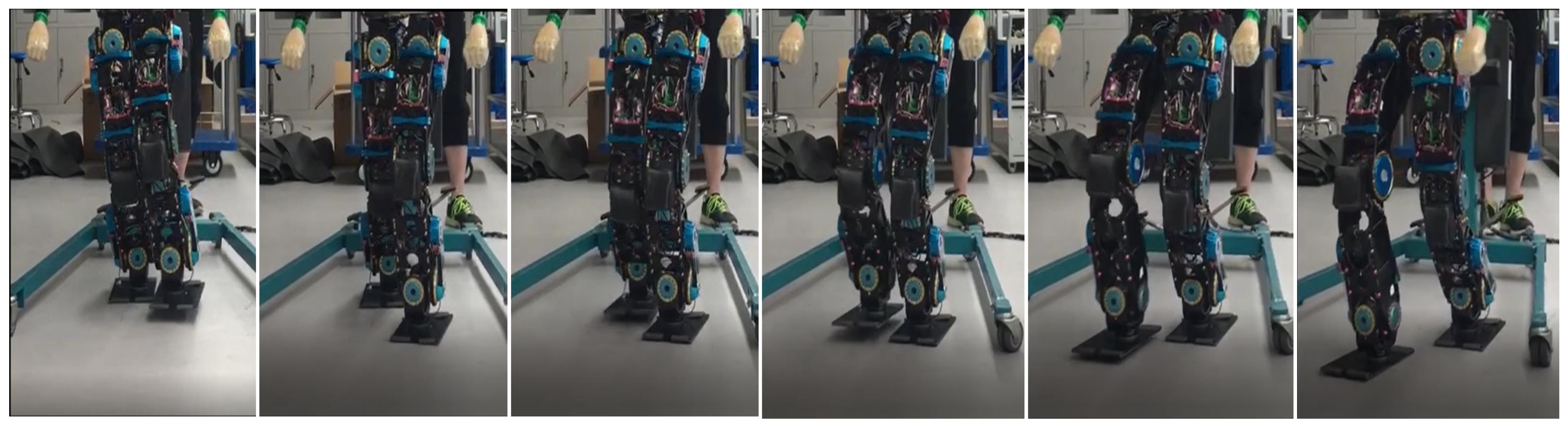
We next applied the proposed method to an actual humanoid robot identical to the one modeled in the simulation platform and under the same parameters as the simulation. As shown in Figure 17, $D_{\mathrm{step}}=0.33\mathrm{m},T_{\mathrm{step}}=1.2$ s, and the robot achieved turning walk at a speed of 1 km/h.

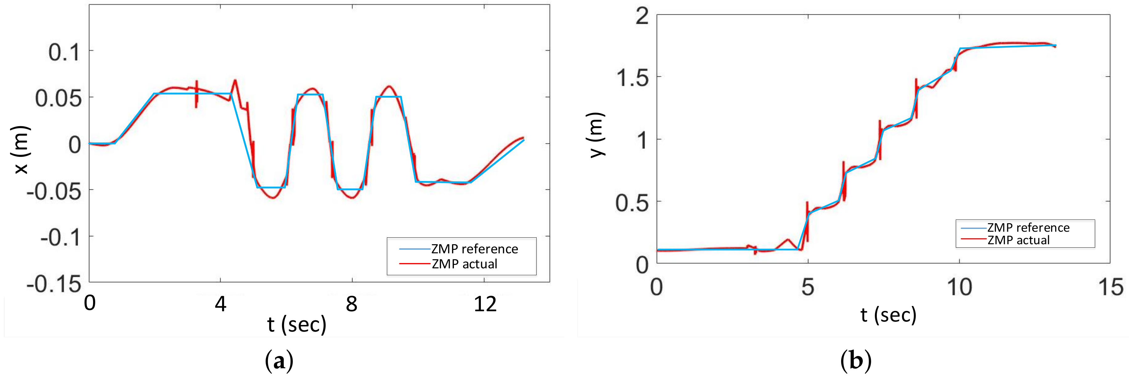
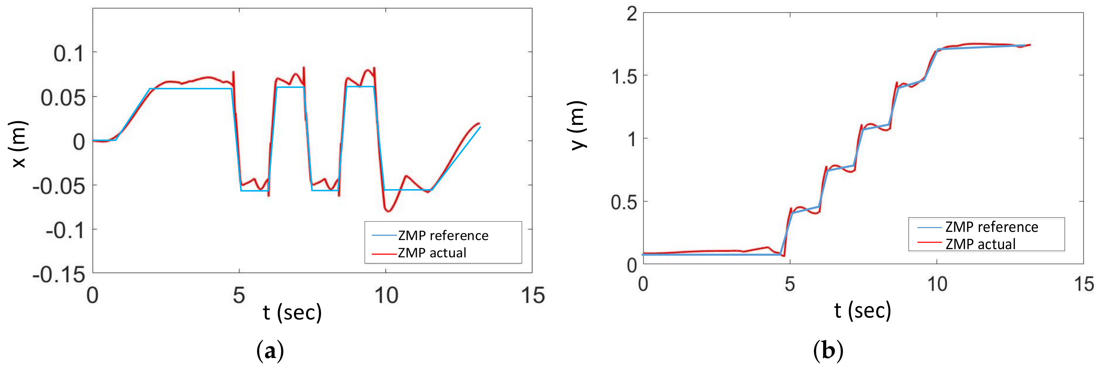
Then, we measured the actual ZMP of the robot calculated by the force sensors and converted it to the IRF, as shown in Figure 18. Another experiment was also done which generated the robot’s COM trajectory directly by the LIP as is shown in Figure 19. By using the proposed method, The actual ZMP trajectory of the robot was able to better follow the planned ZMP both in the lateral direction and the longitudinal direction. This agrees with the results of the simulation results. In the simulation shown in Figure 13, the COM trajectory deviated to one side in order to make the actual ZMP trajectory follow the planned ZMP trajectory. However, the traditional LIP does not take into account the effect of the robot’s own rotation on the actual ZMP, so in the lateral direction, the actual ZMP is offset to one side by a distance form the planned ZMP. In addition, in the longitudinal direction, there are no changes in dynamics, so the actual ZMP can also follow the planned ZMP well.

6. Conclusions

In view of the limitations of the current LIP model in the gait planning of robot turning, we presented a turning walk method for humanoid robots that can reduce the error between the model and the actual robot. This method not only makes the model accurate, but also avoids complex dynamic analysis. By introducing the IRF, the dynamics of the turning walk model were also simplified using the LIP model with centripetal forces acting in the left and right directions. We performed some simulations and experiments to verify the correctness of the proposed method. The results proved that this method can achieve a stable turning walk.

The proposed method involves coordinate system transformations between world coordinate references and the IRF. So when the robot’s COM coordinate and the world coordinate are relatively rotated horizontally, this means the robot will turn and the proposed method will play a part.

Working from another perspective, the straight-line walk can be seen as a special case of the turn walk. For the straight-line walk, the turn radius can be seen as infinity $r_{\mathrm{c}}=\infty$. We can obtain Formula (5) from Formula (6), and $\Delta \alpha$ in Formula (21) has no value, so all the formulas are the same as those in the straight-line walk.

The results show that our method is more effective during rapid turning of a robot which can greatly improve the efficiency of the robot movement. However, for turns with small radii, the calculated turning angle is large, so the robot will easily slip when the robot is also carrying out a fast turn. For the robot slip turn, there has been some research, as is shown in the first section, so the robot can make a slip turn in order to improve efficiency of the turn.

References

- Wieber, P.B. Trajectory free linear model predictive control for stable walking in the presence of strong perturbations. In Proceedings of the IEEE-RAS International Conference on Humanoid Robots, Genova, Italy, 4–6 December 2006; pp. 137–142. [Google Scholar]
- Pratt, J.; Carff, J.; Drakunov, S.; Goswami, A. Capture point: A step toward humanoid push recovery. In Proceedings of the IEEE-RAS International Conference on Humanoid Robots, Genova, Italy, 4–6 December 2006; pp. 200–207. [Google Scholar]
- Herdt, A.; Perrin, N.; Wieber, P.B. Walking without thinking about it. In Proceedings of the IEEE/RSJ International Conference on Intelligent Robots and Systems, Taipei, Taiwan, 18–22 October 2010; pp. 190–195. [Google Scholar]
- Morisawa, M.; Kajita, S.; Kanehiro, F.; Kaneko, K.; Miura, K.; Yokoi, K. Balance control based on capture point error compensation for biped walking on uneven terrain. In Proceedings of the IEEE-RAS International Conference on Humanoid Robots (Humanoids), Osaka, Japan, 29 November–1 December 2012; pp. 734–740. [Google Scholar]
- Deits, R.; Tedrake, R. Footstep planning on uneven terrain with mixed-integer convex optimization. In Proceedings of the IEEE-RAS International Conference on Humanoid Robots, Madrid, Spain, 18–20 November 2014; pp. 279–286. [Google Scholar]
- Kajita, S.; Kanehiro, F.; Kaneko, K.; Fujiwara, K.; Harada, K.; Yokoi, K.; Hirukawa, H. Biped walking pattern generation by using preview control of zero-moment point. In Proceedings of the International Conference on Robotics and Automation, Taipei, Taiwan, 14–19 September 2003; Volume 2, pp. 1620–1626. [Google Scholar]
- Lanari, L.; Hutchinson, S.; Marchionni, L. Boundedness issues in planning of locomotion trajectories for biped robots. In Proceedings of the IEEE-RAS International Conference on Humanoid Robots, Madrid, Spain, 18–20 November 2014; pp. 951–958. [Google Scholar]
- Huang, Q.; Yokoi, K.; Kajita, S.; Kaneko, K.; Arai, H.; Koyachi, N.; Tanie, K. Planning walking patterns for a biped robot. IEEE Trans. Robot. Autom. 2001, 17, 280–289. [Google Scholar] [CrossRef] [Green Version]
- Koolen, T.; Boer, T.D.; Rebula, J.; Goswami, A.; Pratt, J. Capturability-based analysis and control of legged locomotion, Part 1: Theory and application to three simple gait models. Int. J. Robot. Res. 2012, 31, 1094–1113. [Google Scholar] [CrossRef]
- Mombaur, K.; Truong, A.; Laumond, J.P. From Human to Humanoid Locomotion—An Inverse Optimal Control Approach; Kluwer Academic Publishers: Norwell, MA, USA, 2010. [Google Scholar]
- Faraji, S.; Pouya, S.; Ijspeert, A. Robust and Agile 3D Biped Walking With Steering Capability Using a Footstep Predictive Approach. In Proceedings of the Robotics Science and Systems (RSS), Berkeley, CA, USA, 12–16 July 2014. [Google Scholar]
- Sulistijono, I.A.; Setiaji, O.; Salfikar, I.; Kubota, N. Fuzzy walking and turning tap movement for humanoid soccer robot EFuRIO. In Proceedings of the IEEE International Conference on Fuzzy Systems, Barcelona, Spain, 18–23 July 2010; pp. 1–6. [Google Scholar]
- Hu, Y.; Mombaur, K. Bio-Inspired Optimal Control Framework to Generate Walking Motions for the Humanoid Robot iCub Using Whole Body Models. Appl. Sci. 2018, 8, 278. [Google Scholar] [CrossRef]
- Han, B.; Luo, X.; Liu, Q.; Zhou, B.; Cheng, X. Hybrid control for SLIP-based robots running on unknown rough terrain. Robotica 2014, 32, 1065–1080. [Google Scholar] [CrossRef]
- Shahbazi, M.; Babuska, R.; Lopes, G.A.D. Unified Modeling and Control of Walking and Running on the Spring-Loaded Inverted Pendulum. IEEE Trans. Robot. 2016, 32, 1178–1195. [Google Scholar] [CrossRef]
- Poulakakis, I. Spring Loaded Inverted Pendulum embedding: Extensions toward the control of compliant running robots. Robot. Autom. 2010, 58, 5219–5224. [Google Scholar]
- Cao, Y.; Suzuki, S.; Hoshino, Y. Turn Control of a Three-Dimensional Quasi-Passive Walking Robot by Utilizing a Mechanical Oscillator. Engineering 2014, 6, 93–99. [Google Scholar] [CrossRef]
- Miura, K.; Kanehiro, F.; Kaneko, K.; Kajita, S.; Yokoi, K. Slip-Turn for Biped Robots. IEEE Trans. Robot. 2013, 29, 875–887. [Google Scholar] [CrossRef]
- Miura, K.; Kanehiro, F.; Harada, K.; Kaneko, K.; Yokoi, K.; Kajita, S. Slip turn generatioin of humanoid robots based on an analysis of friction model. In Emerging Trends in Mobile Robotics; World Scientific: Singapore, 2015; pp. 761–768. [Google Scholar]
- Miura, K.; Kanehiro, F.; Kaneko, K.; Kajita, S.; Yokoi, K. Quick slip-turn of HRP-4C on its toes. In Proceedings of the IEEE International Conference on Robotics and Automation, Saint Paul, MN, USA, 14–18 May 2012; pp. 3527–3528. [Google Scholar]
- Koeda, M.; Ueno, M.; Serizawa, T. Shuffle Parallel Translation and Pivot Turn of Humanoid Robot in Dynamics Simulator. In Proceedings of the International Conference on Artificial Intelligence, Modelling and Simulation (AIMS), Kota Kinabalu, Malaysia, 3–5 December 2013; pp. 217–220. [Google Scholar]
- Hashimoto, K.; Yoshimura, Y.; Kondo, H.; Lim, H.-O.; Takanishiet, A. Realization of quick turn of biped humanoid robot by using slipping motion with both feet. In Proceedings of the IEEE International Conference on Robotics and Automation, Shanghai, China, 9–13 May 2011; pp. 2041–2046. [Google Scholar]
- Peng, S.; Shui, H.; Ma, H. A simulation and experiment research on turning gait planning of blackmann-II humanoid robot. In Proceedings of the IEEE International Conference on Control and Automation, Xiamen, China, 9–11 June 2010; pp. 719–724. [Google Scholar]
- Kajita, S.; Hirukawa, H.; Harada, K.; Yokoi, K. Introduction to Humanoid Robotics; Springer Publishing Company: Berlin, Germany, 2014. [Google Scholar]
- Scianca, N.; Cognetti, M.; de Simone, D.; Lanari, L.; Oriolo, G. Intrinsically stable MPC for humanoid gait generation. In Proceedings of the IEEE-RAS 16th International Conference on Humanoid Robots, Cancun, Mexico, 15–17 November 2016; pp. 601–606. [Google Scholar]
Figure 1.
Non-inertial Reference in turning walking.
Figure 2.
Force analysis in a non-inertial frame.
Figure 3.
Different radii of the robot turning walk.
Figure 4.
Linear inverted pendulum of the robot.
Figure 5.
Model of the linear inverted pendulum (LIP) of the robot’s turning walk in the x direction.
Figure 6.
Transformation between straight and turning walk.
Figure 7.
Foot position planning.
Figure 8.
Hip yaw joint.
Figure 9.
AZR of the double support period.
Figure 10.
Rotation angle of the center of mass (COM) coordinate system.
Figure 11.
ZMP planning for the robot turning walk.
Figure 12.
COM trajectories: (a) km/h, (b) , (c) , (d) .
Figure 13.
COM trajectories in the involute reference frame (IRF) (a) km/h, (b) km/h.
Figure 14.
The value of the : (a) km/h, (b) km/h, (c) km/h, (d) km/h.
Figure 15.
Hip yaw angle characteristics.
Figure 16.
Angle data for gait planning.
Figure 17.
Experiments in the real humanoid robot.
Figure 18.
ZMP reference vs. actual with proposed method (a): Lateral ZMP, (b): Longitudinal zero moment point (ZMP).
Figure 19.
ZMP reference vs. actual with previous LIP (a): Lateral ZMP, (b): Longitudinal ZMP.