Trajectory Tracking between Josephson Junction and Classical Chaotic System via Iterative Learning Control

Abstract

This article addresses trajectory tracking between two non-identical systems with chaotic properties. To study trajectory tracking, we used the Rossler chaotic and resistive-capacitive-inductance shunted Josephson junction (RCLs-JJ) model in a similar phase space. In order to achieve goal tracking, two stages were required to approximate target tracking. The first stage utilizes the active control technique to transfer the output signal from the RCLs-JJ system into a quasi-Rossler system. Next, the RCLs-JJ system employs the proposed iterative learning control scheme in which the control signals are from the drive system to trace the trajectory of the Rossler system. The numerical results demonstrate the validity of the proposed method and the tracking system is asymptotically stable.

1. Introduction

Chaotic phenomena in semi-conductor devices found in the radio-frequency-base (rf-base) resistive-capacitive shunted Josephson Junction (RCs-JJ) were described by Kautz and Monaco [1] in the numerical study of three system parameters. Many studies have exhibited the chaotic behavior in superconducting resistive-capacitive-inductance Josephson Junction (RCLs-JJ) systems [2,3,4]. The properties of RCLs-JJ including the homo-clinic, hetero-clinic, and super-harmonic bifurcations have been investigated to be excited by these varying parameters [5]. The damped pendulum equation describes the junction behavior and demonstrates the chaotic strange attractor in the phase space [6]. Synchronization is a significant topic, which was based on studying the tracking trajectory in chaotic systems. A non-linear controller by utilizing the back-stepping technique has been investigated to control bifurcation in the RCLs-JJ system [7]. The chaos synchronization between two identical RCLs-JJ systems has been examined in which a number of different techniques to design the controller such as using active control [8], utilizing a common chaos to drive RCLs-JJ system approaching synchronization [9], applying the back-stepping [10,11,12,13], and using the time-delay feedback control [14], respectively. In other studies, the controller design or controller rule is directly determined by the Lyapunov function [11,12] and the RCLs-J junctions array synchronization [12].

Recently, the reconstruction of chaotic systems is similar to chaotic synchronization where the chaotic system was reconstructed from the unknown input [15,16,17]. The chaotic systems synchronization utilized unknown inputs observed in the Takagi-Sugeno (T-S) fuzzy model [15]. The Takagi-Sugeno (T-S) fuzzy model with unknown inputs applied the Lyapunov function and the Linear Matrix Inequalities (LMI) constraint approaching a zero synchronization error in secure communication [16]. The evolutionary algorithms based on the measured data without any internal partial knowledge to reconstruct chaotic systems and demonstrates the numerical results in Reference [17].

In many studies, synchronization systems in the state space model for superconductor devices were described in identical RCLs-Josephson junction systems. Classical non-identical system synchronization is not meant to handle a superconducting system. Accordingly, many trajectory tracking studies have rarely been directly based on the RCLs-JJ system and classical chaotic systems together. This article focuses on the trajectory tracking between two non-identical systems in which one of the systems is the classical chaos system of the Rossler and the other is the RCLs-JJ model in state space representing a mesoscopic system. In this research, two stages tracking the trajectory method uses the RCLs-JJ system in the state space model to trace the trajectory of the Rossler system. The first tracking stage utilizes the active control technique [18] to transfer the RCLs-JJ system into the quasi-Rossler system. In the next stage, the proposed iterative learning control law approaches the trajectory of the Rossler system by correcting the repetition tolerance from the preceded output information between the quasi-Rossler system and the Rossler system [12]. The RCLs-JJ system becomes the quasi-Rossler system and employs the iterative learning control (ILC) procedure to control signals from the Rossler system to trace the trajectory of the drive system. However, most ILC research update rules are designed based on the linear ILC law. The varying reference input [19] is very different from the chaotic signals, which are unexpected. Nevertheless, chaotic systems are unpredictable and can be synchronized [20,21] by designing a controller. The challenges involve extracting the message embedded within the chaotic signal from the normal signal of the regular system such as a digital encoding system. A chaotic signal cannot implement the code by the obvious method. The chaotic synchronization should lead to a secure communication system by using a synchronized chaotic electronic circuit [22].

In this study, the chaotic tracking trajectory that utilized the ILC method based on the Josephson junction chaos can also employ other methods such as a backstepping controller [7], an active control [8], a common chaos driving by Rossler [9], and LMI [16] and we examine the results. This article provides two main contributions. The first is a real-time feedforward procedure that uses iterative learning to modify the trajectory error between systems for tracking two non-identical systems. A few studies have been published on two different chaotic systems directly tracking or synchronizing. However, reports are especially rare for Josephson Junction systems and classical chaotic systems. Another contribution is the utility of the synchronization or minimum tracking error leads to the secure communication system by applying the Josephson Junction systems into quantum chaotic systems to deliver the message in the communication system.

The organization of this paper is explained. The next section describes the Rossler Chaotic and RCL-Shunted Josephson Junction system. Section 3 outlines the simulation results and provides an example to demonstrate the proposed learning control law in the RCLs-JJ system to trace the path of the Rossler system. Lastly, this paper highlights the future applications and conclusions in Section 4.

2. Rossler Chaotic and RCL-Shunted Josephson Junction System

2.1. System Description and Transformation

The Rossler chaotic system has an initial condition X₀, which is the drive system in a general form.

$$\dot{\mathit{X}}=\mathit{A}\mathit{X}+\mathit{b}=\left[\begin{array}{ccc}0& -1& -1\\ 1& a& 0\\ 0& 0& x_1-c\end{array}\right]\left[\begin{array}{c}{x}_1\\ x_2\\ x_3\end{array}\right]+\left[\begin{array}{c}0\\ 0\\ b\end{array}\right]$$

(1)

$\mathit{X}={\left[\begin{array}{ccc}{x}_1,& x_2,& x_3\end{array}\right]}^T$ is the state vector. The RCLs-JJ can be expressed by Equation (2) with initial conditions Y₀ = [0 0 0]^T.

$$\dot{\mathit{Y}}=\mathit{B}\mathit{Y}+\mathit{b}\psi \left(y_1\right)+{\mathit{U}}^{\left(k\right)}$$

(2)

where $\mathit{Y}={\left[\begin{array}{ccc}{y}_1& y_2& y_3\end{array}\right]}^T$ and

$$\mathit{B}=\left[\begin{array}{ccc}0& 1& 0\\ 0& -\frac{g\left(y_2\right)}{{\beta }_C}& \frac{1}{{\beta }_C}\\ 0& \frac{1}{{\beta }_L}& -\frac{1}{{\beta }_L}\end{array}\right],\hspace{1em}\mathit{b}=\left[\begin{array}{c}0\\ \frac{1}{{\beta }_C}\\ 0\end{array}\right],\hspace{1em}\psi \left(y_1\left(t\right)\right)=i_N-\sin \left(y_1\right).$$

(3)

where $g\left(y_2\right)$ is given by

$$g\left(y_2\right)=\{\begin{array}{l}0.366 \mathrm{as} \left|y_2\right|>2.9\\ 0.061 \mathrm{as} \left|y_2\right|\le 2.9,\end{array}$$

(4)

k in Equation (2) is the iterative number that uses the iterative learning control law (ILC) as shown in the equation below.

$${\mathit{U}}^{\left(k\right)}={\left[\begin{array}{ccc}{v}_{\mathrm{a}}& v_{\mathrm{b}}& v_{\mathrm{c}}\end{array}\right]}^{\mathrm{T}}+{\left[\begin{array}{ccc}{u}_1^{\left(k\right)}& u_2^{\left(k\right)}& u_3^{\left(k\right)}\end{array}\right]}^{\mathrm{T}}$$

(5)

The ILC rule is a sequence of the control input signal for the response system as ${\left\{{\mathit{U}}^{\left(k\right)}\right\}}_{k=1,2,\cdots }$.

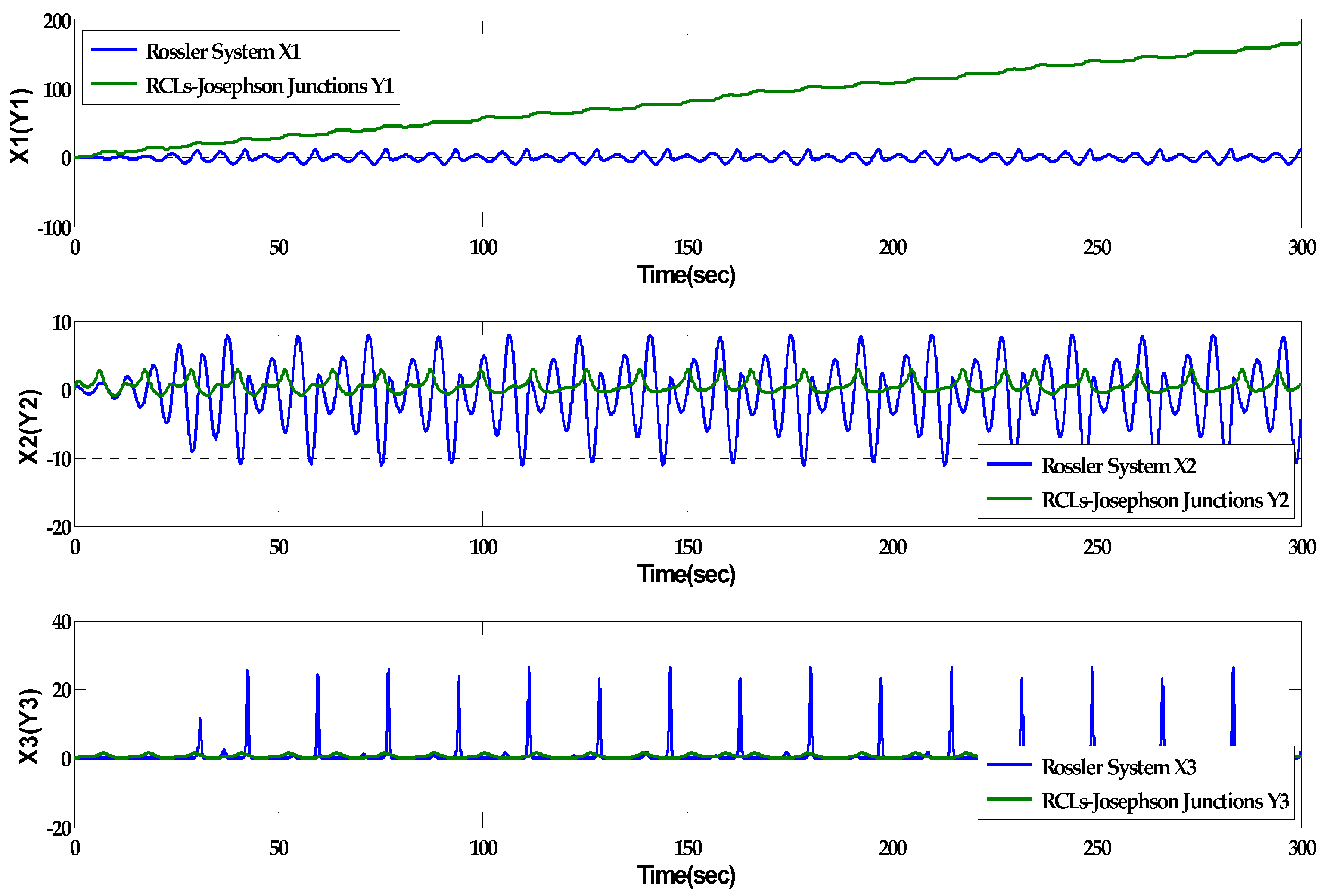
Equations (1) and (2) are nearly non-identical nonlinear systems, which is seen by their trajectory in Figure 1.

Figure 1 displays the time response of the state of two distinct systems known as the Rossler and the RCLs-JJ systems with different initial states. The trajectory error between the systems in each state should be enormous in Figure 1. The nonlinear system in Equation (2) should be transferred to the quasi-Rossler system to track the trajectory of the system in Equation (1). Therefore, the active control technique [23,24] is utilized in Equation (2).

According to the active control technique, the description of the system in Equation (2) and the dynamic transformation between the drive in Equation (1) and the response system in Equation (2) is shown in the equation below.

$$\mathit{z}=\left[\begin{array}{c}{z}_a\\ z_b\\ z_c\end{array}\right]=\left[\begin{array}{c}{y}_1-x_1\\ y_2-x_2\\ y_3-x_3\end{array}\right]$$

(6)

$$\begin{array}{l}\dot{\mathit{z}}=\left[\begin{array}{c}{\dot{z}}_a\\ {\dot{z}}_b\\ {\dot{z}}_c\end{array}\right]=\left[\begin{array}{c}{\dot{y}}_1-{\dot{x}}_1\\ {\dot{y}}_2-{\dot{x}}_2\\ {\dot{y}}_3-{\dot{x}}_3\end{array}\right]\\ =\left[\begin{array}{c}{z}_b+2x_2+x_3\\ \frac{-1}{{\beta }_{\mathrm{C}}}g\left(y_2\right)z_b+\frac{1}{{\beta }_C}{z}_c+\frac{1}{{\beta }_{\mathrm{C}}}\left[i_N-\sin (y_1)\right]-x_1-\left(a+\frac{g\left(y_2\right)}{{\beta }_{\mathrm{C}}}\right)x_2-\frac{x_3}{{\beta }_{\mathrm{C}}}\\ \frac{1}{{\beta }_{\mathrm{L}}}{z}_b-\frac{1}{{\beta }_{\mathrm{L}}}{z}_c+\frac{1}{{\beta }_{\mathrm{L}}}\left(x_2-x_3\right)-x_1{x}_3-c{x}_3-b\end{array}\right]+\left[\begin{array}{c}{v}_{\mathrm{a}}\\ v_{\mathrm{b}}\\ v_{\mathrm{c}}\end{array}\right]\end{array}$$

(7)

where ${\left[\begin{array}{ccc}{v}_a& v_b& v_c\end{array}\right]}^T$ is the active control function that eliminates the terms that have no $z_i$ for i = a, b, c. As a result, the active control function can be determined by the equation below.

$$\left[\begin{array}{c}{v}_a\\ v_b\\ v_c\end{array}\right]=\left[\begin{array}{c}-2x_2-x_3\\ \frac{-1}{{\beta }_{\mathrm{C}}}\left[i_N-\sin (y_1)\right]+x_1+\left(a+\frac{g\left(y_2\right)}{{\beta }_{\mathrm{C}}}\right)x_2+\frac{x_3}{{\beta }_{\mathrm{C}}}\\ \frac{-1}{{\beta }_{\mathrm{L}}}\left(x_2-x_3\right)+x_1{x}_3+c{x}_3+b\end{array}\right]+\left[\begin{array}{c}{w}_{\mathrm{a}}\\ w_{\mathrm{b}}\\ w_{\mathrm{c}}\end{array}\right]$$

(8)

where ${\left[\begin{array}{ccc}{w}_a& w_b& w_c\end{array}\right]}^T$ is the error term in the active control procedure. Substituting Equation (8) into (7), Equation (7) was transformed into the formula below.

$$\dot{\mathit{z}}=\left[\begin{array}{c}{\dot{z}}_a\\ {\dot{z}}_b\\ {\dot{z}}_c\end{array}\right]=\left[\begin{array}{c}{z}_b\\ \frac{-1}{{\beta }_{\mathrm{C}}}g\left(y_2\right)z_b-\frac{1}{{\beta }_C}{z}_c\\ \frac{1}{{\beta }_{\mathrm{L}}}{z}_b-\frac{1}{{\beta }_{\mathrm{L}}}{z}_c\end{array}\right]+\left[\begin{array}{c}{w}_a\\ w_b\\ w_c\end{array}\right]$$

(9)

The matrix form of Equation (8) can be rewritten as the formula below.

$$\dot{\mathit{z}}=\left[\begin{array}{c}{\dot{z}}_a\\ {\dot{z}}_b\\ {\dot{z}}_c\end{array}\right]=\mathit{A}\left[\begin{array}{c}{z}_a\\ z_b\\ z_c\end{array}\right]+\left[\begin{array}{c}{w}_{\mathrm{a}}\\ w_{\mathrm{b}}\\ w_{\mathrm{c}}\end{array}\right]$$

(10)

Suppose the matrix A has eigenvalues $\left({\lambda }_a,{\lambda }_{b,}{\lambda }_c\right)=\left(-1,-1,-1\right)$. Then the characteristic equations of A are demonstrated by the equation below.

$$\left[\begin{array}{ccc}-1& -1& 0\\ 0& -1+\frac{1}{{\beta }_{\mathrm{C}}}g\left(y_2\right)& \frac{1}{{\beta }_{\mathrm{C}}}\\ 0& \frac{-1}{{\beta }_{\mathrm{L}}}& -1+\frac{1}{{\beta }_{\mathrm{L}}}\end{array}\right]\left[\begin{array}{c}{z}_a\\ z_b\\ z_c\end{array}\right]=\left[\begin{array}{c}{w}_a\\ w_b\\ w_c\end{array}\right]$$

(11)

The solution of ${\left[\begin{array}{ccc}{w}_a& w_b& w_c\end{array}\right]}^T$ is shown below.

$$\left[\begin{array}{c}{w}_a\\ w_b\\ w_c\end{array}\right]=\left[\begin{array}{c}-z_a-z_b\\ -\left(1-\frac{1}{{\beta }_{\mathrm{C}}}g\left(y_2\right)\right)z_b+\frac{1}{{\beta }_{\mathrm{C}}}{z}_c\\ \frac{-1}{{\beta }_{\mathrm{L}}}{z}_b-\left(1-\frac{1}{{\beta }_{\mathrm{L}}}\right)z_c\end{array}\right]$$

(12)

Equation (9) used Equation (12) to become ${\left[\begin{array}{ccc}{\dot{z}}_a& {\dot{z}}_b& {\dot{z}}_c\end{array}\right]}^T={\left[\begin{array}{ccc}-z_a& -z_b& -z_c\end{array}\right]}^T$. By substituting Equations (12) and (8) into the RCLs-Josephson Junction system in Equation (2) with an iterative learning control rule and changing the variable x to variable y, the system became the formula below.

$$\dot{\mathit{Y}}=\left[\begin{array}{c}-y_2-y_3-z_a\\ y_1+a{y}_2-z_b\\ y_1{x}_3-c{y}_3-z_c\end{array}\right]+{\mathit{U}}^{\left(k\right)}=\left[\begin{array}{ccc}0& -1& -1\\ 1& a& 0\\ 0& 0& y_1-c\end{array}\right]\left[\begin{array}{c}{y}_1\\ y_2\\ y_3\end{array}\right]+\left[\begin{array}{c}0\\ 0\\ b\end{array}\right]-\left[\begin{array}{c}{z}_a\\ z_b\\ z_c\end{array}\right]+\left[\begin{array}{c}{u}_1^{\left(k\right)}\\ u_2^{\left(k\right)}\\ u_3^{\left(k\right)}\end{array}\right]$$

(13)

After the active control procedure, the RCLs-JJ system becomes a quasi-Rossler chaotic system so that the trajectory tracing between different systems traces the trajectory under identical systems.

2.2. Trajectory Tracking between Systems via the Iterative Learning Control

The RCLs-JJ system has now became the quasi-Rossler chaotical system. The ILC procedure and control signal from the drive system utilizes the response system to track the drive system. When an appropriated ${\left\{U^{\left(k\right)}\right\}}_{k=1,2,\cdots }$ is found and the iteration number k is sufficient, the tracked error dynamic system should be equal to zero, that is ${\dot{e}}^{\left(k\right)}\left(t\right)=\underset{k\to \infty }{\lim }\left|\dot{X}\left(t\right)-\dot{Y}\left(t\right)\right|=0$. The tracking trajectory has changed to two similar systems.

In many studies, the synchronization between identical systems employ the control signal from the drive system [25,26,27]. Accordingly, The RCLs-JJ system in Equation (2) uses the control signals from the drive system, x₁ and x₃, which can be rewritten as the equation below.

$$\dot{\mathit{Y}}=\left[\begin{array}{c}{\dot{y}}_1\\ {\dot{y}}_2\\ {\dot{y}}_3\end{array}\right]=\left[\begin{array}{c}{x}_2\\ \frac{1}{{\beta }_{\mathrm{C}}}\left[i_N-g\left(y_2\right)x_2-\sin (y_1)-x_3\right]\\ \frac{1}{{\beta }_{\mathrm{L}}}\left(x_2-x_3\right)\end{array}\right]+{\mathit{U}}^{\left(k\right)}$$

(14)

The control signals from the Rossler system of Equation (14) are similar to the quasi-Ross system in Equation (13) and the iterative learning control law ${\mathit{U}}^{\left(k\right)},$ which is defined by error dynamics. The dynamic error system between the Rossler system in Equation (1) and the quasi-Rossler system in Equation (13) can be exhibited by the formula below.

$$\begin{array}{cc}\hfill \dot{\mathit{e}}=\left[\begin{array}{c}-e_1-e_2\\ e_1+a{e}_2\\ x_3{e}_1-c{e}_3\end{array}\right]& -\left[\begin{array}{c}{z}_a\\ z_b\\ z_c\end{array}\right]+\left[\begin{array}{c}{u}_1^{\left(k\right)}\\ u_2^{\left(k\right)}\\ u_3^{\left(k\right)}\end{array}\right]\hfill \\ & =\left[\begin{array}{ccc}0& -1& -1\\ 1& a& 0\\ 0& 0& -c\end{array}\right]\left[\begin{array}{c}{e}_1\\ e_2\\ e_3\end{array}\right]+\mathit{M}\left(x_i,y_{\mathrm{j}}\right)\mathit{G}\left(\mathit{e}\right)-\left[\begin{array}{c}{z}_a\\ z_b\\ z_c\end{array}\right]+\left[\begin{array}{c}{u}_1^{\left(k\right)}\\ u_2^{\left(k\right)}\\ u_3^{\left(k\right)}\end{array}\right]\hfill \end{array}$$

(15)

The ILC rule ${\mathit{u}}^{\left(k\right)}$ is outlined in References [16,21].

$${\mathit{u}}^{\left(k\right)}={\mathit{B}}_2{\Delta }^{\left(k\right)}+{\mathit{B}}_1{\mathit{u}}^{\left(k-1\right)}$$

(16)

where the matrix ${\mathit{B}}_1={\left(\mathit{M}\right)}^m\ast \left(realeig({\mathit{B}}_2\right){)}^{-n}$ with 0 $\le m\le$ 1, and $1\le n<k$. ${\mathit{B}}_2$ is the coefficient matrix of ${\Delta }^{\left(k\right)}={\left[\begin{array}{ccc}{e}_1& e_2& e_3\end{array}\right]}^T$ in Equation (15) and $realeig({\mathit{B}}_2)$ is the real part of eigenvalue of ${\mathit{B}}_2$. When the $z_{i=a,b,c}=e_{j=1,2,3}$, the term $\mathit{M}\left(x_i,y_{\mathrm{j}}\right)\mathit{G}\left(\mathit{e}\right)$ in Equation (14) can absorb the ${\left[\begin{array}{ccc}{z}_a& z_b& z_c\end{array}\right]}^T$ to choose the appropriate matrix M. By induction, the expansion of ${\mathit{u}}^{\left(k\right)}$ in Equation (16) can be written as the equation below.

$$u^{\left(k\right)}={\left(B_1\right)}^k{u}^{\left(0\right)}+{\left(B_1\right)}^{k-1}{B}_2{\Delta }^{\left(1\right)}+{\left(B_1\right)}^{k-2}{B}_2{\Delta }^{\left(2\right)}+\cdots +B_1{B}_2{\Delta }^{\left(k-1\right)}+B_2{\Delta }^{\left(k\right)}$$

(17)

2.3. Lyapunov Stability of Systems

Equation (7) may be the dynamical error system in the active control procedure. Therefore, the Lyapunov function is defined by the equation below.

$$\mathit{V}=\frac{1}{2}\left(s_1{z}_a{}^2+s_2{z}_b{}^2+s_3{z}_c{}^2\right)$$

(18)

where $s_{j=1,2,3}$ are constant such that $\dot{V}<0$.

Theorem 1.

The Lyapunov function in the active control procedure, which is used to transfer the RCLs-JJ system in Equation (2) to the quasi-Rossler system in Equation (13), can be defined by Equation (18).

Proof. 

Equation (18) should prove the first derivative is negative and the dynamic system is stable at the equilibrium (0, 0, 0). The first derivative of the Lyapunov function is shown below.

$$\dot{V}=\left(s_1{\dot{z}}_a{z}_a+s_2{\dot{z}}_b{z}_b+s_3{\dot{z}}_c{z}_c\right)$$

(19)

Substituting Equation (12) into Equation (9), ${\left[\begin{array}{ccc}{\dot{z}}_a& {\dot{z}}_b& {\dot{z}}_c\end{array}\right]}^T={\left[\begin{array}{ccc}-z_a& -z_b& -z_c\end{array}\right]}^T$, and taking $s_1=s_2=s_3=1$, the following formula is found.

$$\dot{V}=-\left(z_a{}^2+z_b{}^2+z_c{}^2\right)\le 0$$

(20)

☐

Theorem 2.

Based on the ${\mathit{u}}^{\left(\mathit{k}\right)}$in Equation (16), the Lyapunov function is defined in the iterative control stage to trace the trajectory of the Rossler system below.

$$V=\frac{1}{2}\left(r_1{e}_1{}^2+r_2{e}_2{}^2+r_3{e}_3{}^2\right)$$

(21)

Proof. 

Let ${\mathit{u}}^{\left(\mathit{k}-\mathbf{1}\right)}$ be defined as the formula below.

$${\mathit{u}}^{\left(k-1\right)}={\mathit{B}}_2{\Delta }^{\left(k-1\right)}+\mathit{M}\left(x_i,y_{\mathrm{j}}\right)\mathit{G}\left(\mathit{e}\right)$$

(22)

Applying $-{\mathit{u}}^{\left(k-1\right)}$ to Equation (15), we obtain the error dynamics as $\dot{\mathit{e}}={\left[\begin{array}{ccc}-z_a& -z_b& -z_c\end{array}\right]}^T$. Let $z_{i=a,b,c}=e_{j=1,2,3}$ and $r_{j=1,2,3}$= 1. The Lyapunov function is outlined below.

$$\dot{\mathit{V}}=-\left(e_1{}^2+e_2{}^2+e_3{}^2\right)\le \mathbf{0}$$

(23)

This implies that Equation (15) employs the iterative learning control law, which is asymptotically stable at equilibrium.

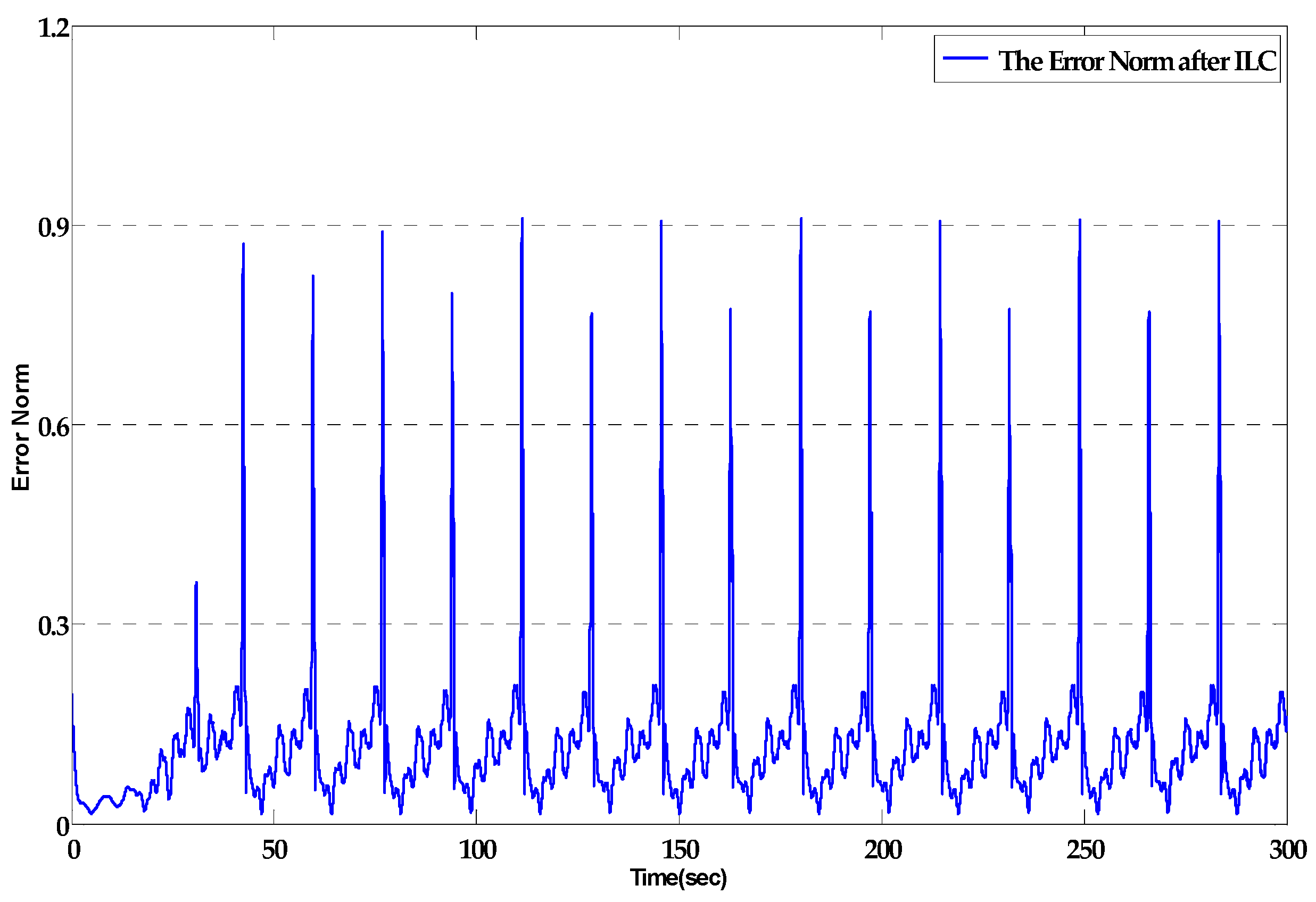
The Lyapunov function is generally a function of the trajectory error or the synchronization error. The error norm can be extended to be a cost function having the lowest cost when the trajectory between systems is close to each other [28,29,30]. The cost function in this work is defined by the formula below.

$$C_F=\left|\right|e_1{}^2+e_2{}^2+e_3{}^2\left|\right|$$

(24)

☐

3. Results and Discussion

To verify the proposed iterative learning control law, we utilize an example to demonstrate the tracing error and trajectory between the Rossler dynamical system in Equation (1) with an initial state (x₁₀, x₂₀, x₃₀) = (0.2, 0.4, 0.1) and the RCLs-JJ system in Equation (2) with an initial state (y₁₀, y₂₀, y₃₀) = (0, 0, 0), respectively.

3.1. Deciding Iterative Control Learning Law

The Rossler system in Equation (1) is given by the formula below.

$$\dot{\mathit{X}}=\mathit{A}\mathit{X}+\mathit{a}=\left[\begin{array}{ccc}0& -1& -1\\ 1& 0.2& 0\\ 0& 0& x_3-5.7\end{array}\right]\left[\begin{array}{c}{x}_1\\ x_2\\ x_3\end{array}\right]+\left[\begin{array}{c}0\\ 0\\ 0.2\end{array}\right],x_0=\left[\begin{array}{c}0.2\\ 0.4\\ 0.1\end{array}\right].$$

(25)

The RCLs-JJ model in Equation (2) is given by the formula below.

$$\dot{\mathit{Y}}=\mathit{B}\mathit{Y}+\mathit{b}\psi \left(y_1\right)+{\mathit{U}}^{\left(k\right)},{\mathit{Y}}_{\mathbf{0}}=\left[\begin{array}{c}0\\ 0\\ 0\end{array}\right]$$

(26)

where the parameters in Equation (25) have been defined in Equations (3) and (4) in which the values of entries in matrix B are β_L = 2.6, β_c = 0.707, i_N = 1.132, and $\psi \left(y_1\right)=1.132-\sin \left(y_1\right)$. The ${\mathit{U}}^{\left(k\right)}$ of the system in Equation (25) is the ILC rule in Equation (5). The ${\mathit{u}}^{\left(k\right)}$ defined in Equation (16) minimizes the tracking error between the Rossler system and the RCLs-JJ system. The matrix $\mathit{M}\left(x_i,y_{\mathrm{j}}\right)$ in Equation (15) and ${\mathit{B}}_{\mathbf{2}}$ of Equation (16) can alternate respectively as the equation below.

$$\mathit{M}\left(x_i,y_{\mathrm{j}}\right)=\left[\begin{array}{ccc}1& 0& 0\\ 0& 1& 0\\ x_1& 0& 1\end{array}\right] \mathrm{and} {\mathit{B}}_{\mathbf{2}}=\left[\begin{array}{ccc}0& 1& 1\\ -1& -0.2& 0\\ -1& 0& 5.7\end{array}\right]$$

(27)

where the $x_1$ is from Rossler system and matrix ${\mathit{B}}_{\mathbf{2}}$ is the decomposition of matrix A in Equation (1). The time interval of the simulation range is from 0 to 300 s and the minimum time step is 0.01 s. This article utilized the program of the Euler method and figures in MATLAB to investigate trajectory tracking by using the ILC law in Equation (17). In the active control procedure, we use the Simulink in MATLAB to transfer the RCLs-JJ system to the Rossler system.

3.2. Exhibiting Simulation Results and Discussion

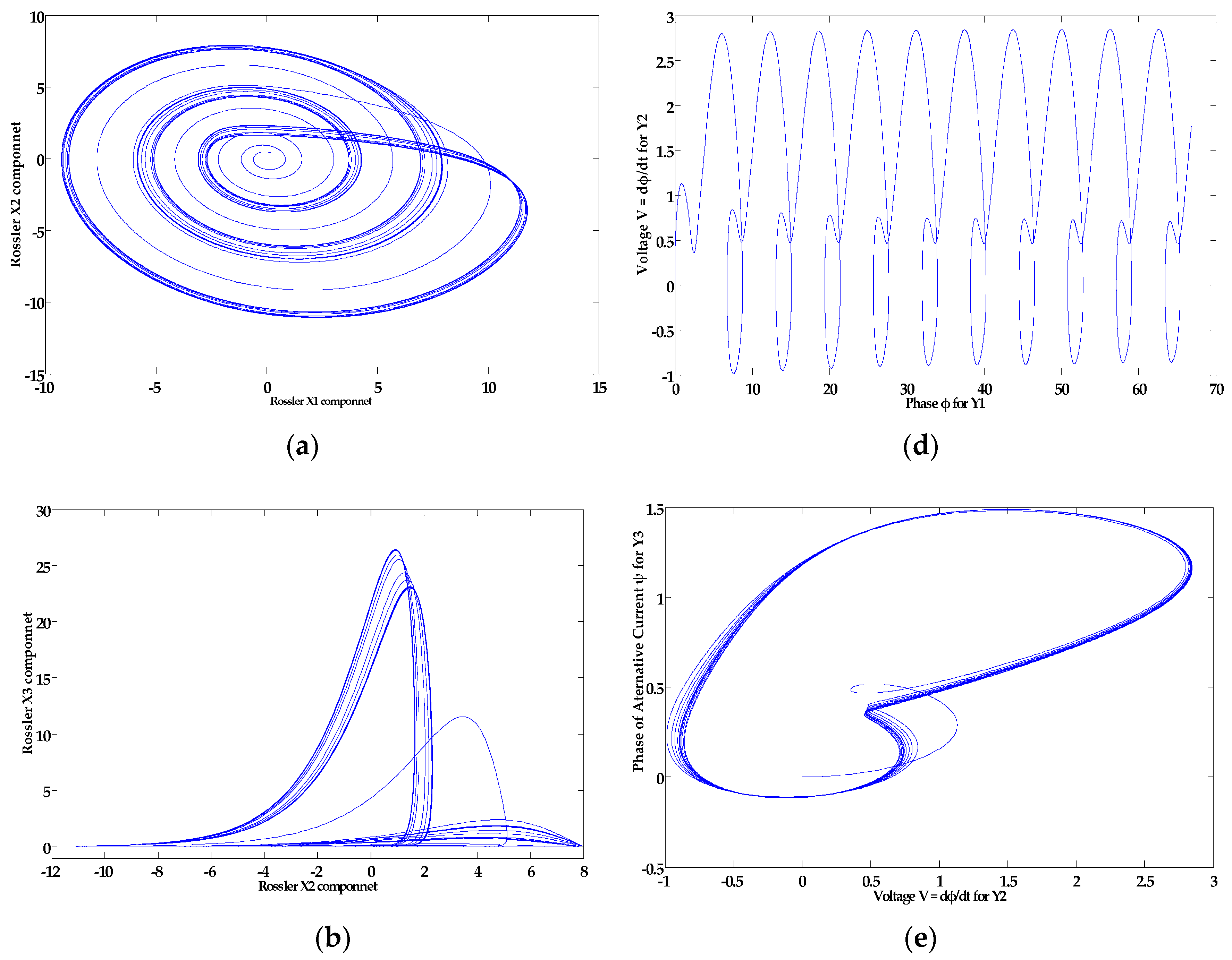
Figure 2 displays two distinct phase portraits of the two systems known as the Rossler and RCLs-JJ systems with different initial states. The chaotic behavior of the Rossler system for each phase portrait is displayed in Figure 2a–c. The phase portrait behaviors of the RCLs-JJ system is shown in Figure 2d–f. The chaotic behavior of the RCLs-JJ system is clear only in Figure 2e and the others are not chaos. The challenge is how to find the controller approach in the minimum trajectory error.

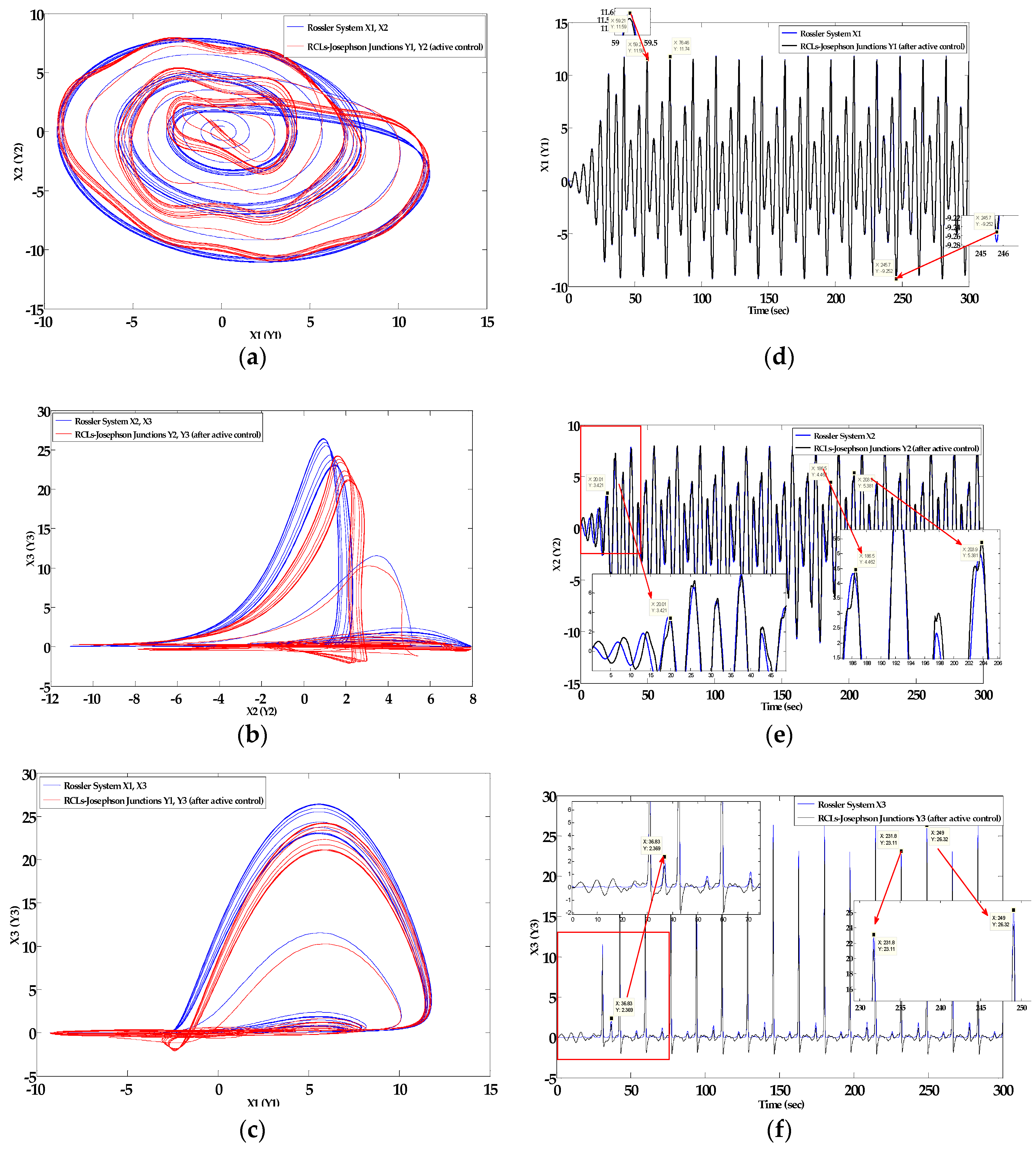
The first stage overcomes the non-identical trajectory between the two systems and employs the active control to change the RCLs-JJ system into a quasi-Rossler system from Equation (6) to Equation (13). The phases of two systems after utilizing the active control technique are exhibited in Figure 3a–c.

The new phase portraits of the RCLs-JJ system are almost completely different from the original phase portraits and are now closer to the Rossler system. Therefore, the new system is called a quasi-Rossler system. The time response of each component of the two systems indicated in Figure 3d–f in the paths of Rossler and RCLs-JJ systems, respectively, are distant from each other.

Figure 4 demonstrates the tracking error between the Rossler and the quasi-Rossler systems, which transfers from the RCLs-JJ system. The vibration of the tracking error has many large amplitudes in the second (y₂-x₂) and third (y₃-x₃) components at the specific moment.

Figure 5 demonstrates the phase portrait of the x₁ (y₁) and x₂ (y₂) by utilizing the ILC update law to track the trajectory. The two trajectories almost overlap, which validates the tracking error phenomena in Figure 6.

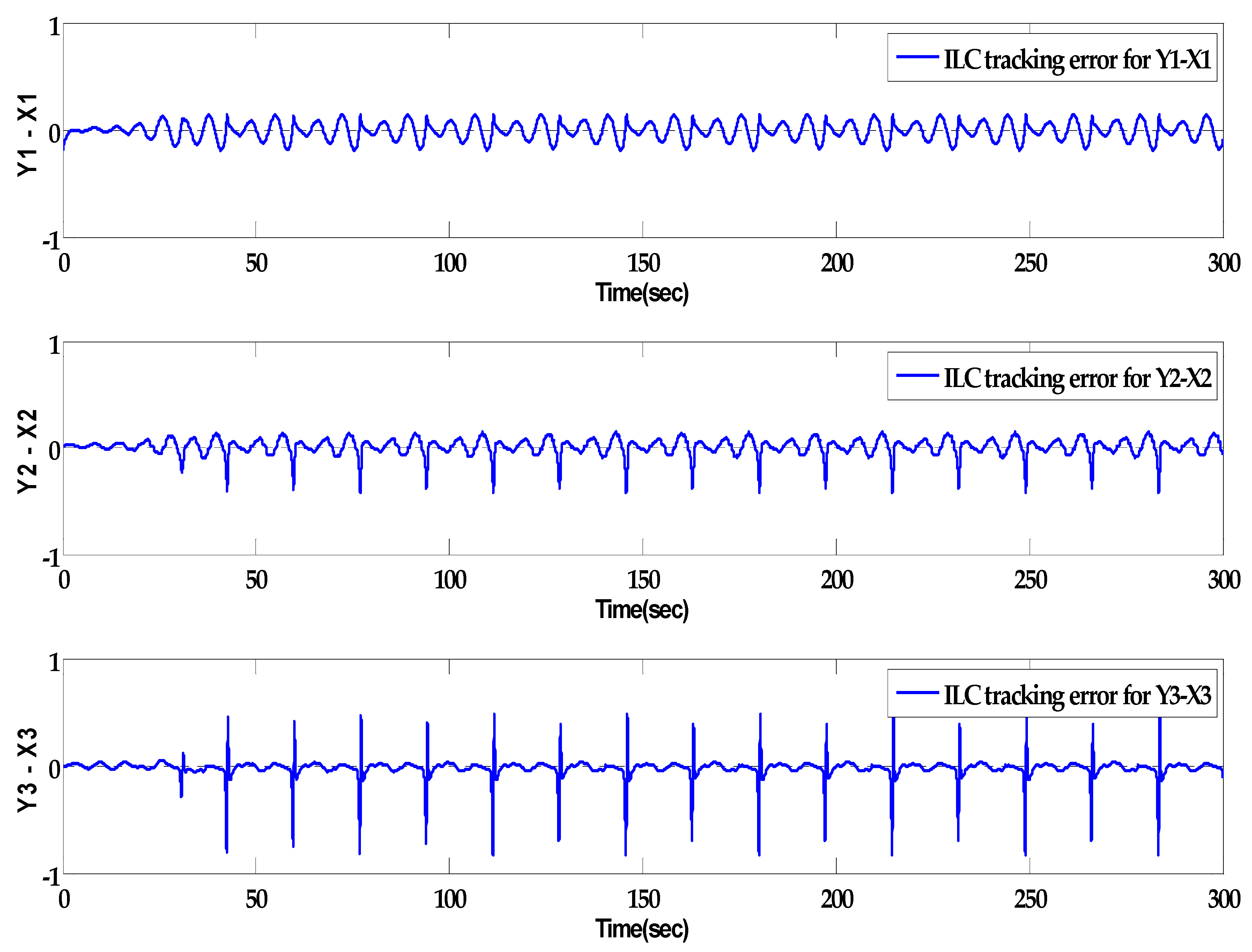
The tracking errors oscillation in Figure 6 are between 0.1408 and −0.1959 for the first tracking error, between 0.1434 and −0.4217 for the second, and between 0.4784 and −0.8344 for the third tracking error, respectively.

Figure 7 exhibits the tracking error after using the ILC law. The third ingredient varies the most when comparing to subfigures in Figure 1. The lager vibration will always occur at a particular moment t_i because the tracking error between two systems became larger at same moments. Comparing Figure 4 and Figure 6, the tracking errors are successfully suppressed between 0.2 and −0.2 for the first two components and the fault of the third component between 0.5 and −0.8 by applying the proposed ILC update law. The error rate is asymptotically stable.

Figure 8 shows the cost function after utilizing the ILC procedure defined by the tracking error norm, which is bounded and less than one. The cost function is created by Figure 4 after applying the divergent active control procedure. The trajectories of the two systems is near each other.

4. Conclusions

This article proposed a learning control law to trace the trajectory between two non-identical nonlinear systems and successfully used a two-stage approach of combining an active control technique and an iterative learning control update law to significantly inhibit and improve the tracking errors in the numerical results. The simulation example helped infer the trajectory tracking process and assert the proposed ILC rule. In this research, the ILC tracking method has been applied to the Josephson junction chaos. Many studies providing other methods such as the backstepping controller [7], the active control [8], common chaos driving by Rossler [9], and LMI [16] should show similar demonstrations.

Future studies should provide a feedforward procedure in a real-time iterative learning process to modify the trajectory error between non-identical systems and apply synchronization or the minimum tracking error procedure into a secure system in quantum communication. The real-time iterative learning procedure would use signal tracking in the deep learning procedure.

References

- Kautz, R.L.; Monaco, R. Survey of chaos in the rf-biased Josephson junction. J. Appl. Phys. 1985, 57, 875. [Google Scholar] [CrossRef]
- Whan, C.B.; Lobb, C.J. Complex dynamical behavior in RCL-shunted Josephson tunnel junctions. Phys. Rev. E 1996, 53, 405–413. [Google Scholar] [CrossRef]
- Dana, S.K.; Sengupta, D.C.; Edoh, K.D. Chaotic Dynamics in Josephson Junction. IEEE Trans. Circuits Syst. Fundam. Theor. Appl. 2001, 48, 1057–7122. [Google Scholar] [CrossRef]
- Hu, Y.T.; Zhou, T.G.; Gu, J.; Yan, S.L.; Fang, L.; Zhao, X.-J. Study on chaotic behaviors of RCLSJ model Josephson junctions. J. Phys. Conf. Ser. 2008, 96, 012035. [Google Scholar] [CrossRef] [Green Version]
- Yuan, S.L.; Jing, Z.J. Bifurcations of periodic solutions and chaos in Josephson system with Parametric Excitation. Acta. Math. Appl. Sin. Engl. Ser. 2015, 31, 335–368. [Google Scholar] [CrossRef]
- Huberman, B.A.; Crutchfield, J.P.; Packard, N.H. Noise phenomena in Josephson junctions. Appl. Phys. Lett. 1980, 37, 750–752. [Google Scholar] [CrossRef]
- Harb, A.M.; Harb, B.A. Controlling Chaos in Josephson-Junction Using Nonlinear Backstepping Controller. IEEE Trans. Appl. Supercond. 2006, 16, 1988–1998. [Google Scholar] [CrossRef]
- Ucar, A.; Lonngren, K.E.; Bai, E.W. Chaos synchronization in RCL-shunted Josephson junction via active control. Chaos Solitons Fractals 2007, 31, 105–111. [Google Scholar] [CrossRef]
- Feng, Y.L.; Shen, K.E. Chaos synchronization in RCL-shunted Josephson junctions via a common chaos driving. Eur. Phys. J. B 2008, 61, 105. [Google Scholar] [CrossRef]
- Vincenta, U.E.; Ucarb, A.; Laoyea, J.A.; Kareema, S.O. Control and synchronization of chaos in RCL-shunted Josephson junction using backstepping design. Physica C 2008, 468, 374–382. [Google Scholar] [CrossRef]
- Zribi, M.; Khachab, N.; Boufarsan, M. Synchronization of two RCL shunted Josephson Junctions. In Proceedings of the 2011 International Conference on Microelectronics (ICM), Hammamet, Tunisia, 19–22 December 2011. [Google Scholar] [CrossRef]
- Lu, C.; Liu, A.; Ling, M.; Dong, E. Synchronization of chaos in RCL-shunted Josephson junctions array. Chin. Autom. Congr. 2015, 1956–1961. [Google Scholar] [CrossRef]
- Njah, A.N.; Ojo, K.S.; Adebayo, G.A.; Obawole, A.O. Generalized control and synchronization of chaos in RCL-shunted Josephson junction using backstepping design. Physica C 2010, 470, 558–564. [Google Scholar] [CrossRef]
- Xu, S.Y.; Tang, Y.; Sun, H.D.; Zhou, Z.G.; Yang, Y. Characterizing the anticipating chaotic synchronization of RCL-shunted Josephson junctions. Int. J. Non-Linear Mech. 2012, 47, 1124–1131. [Google Scholar] [CrossRef]
- Chadli, M.; Zekinka, L.; Yousset, T. Unknown inputs observer design for fuzzy systems with application to chaotic system reconstruction. Comput. Math. Appl. 2013, 66, 147–154. [Google Scholar] [CrossRef]
- Chadli, M.; Zekinka, L. Chaos synchronization of unknown inputs Takagi-Sugeno fuzzy: Application to secure communications. Comput. Math. Appl. 2014, 68, 2142–2147. [Google Scholar] [CrossRef]
- Zekinka, L.; Chadli, M.; Davendra, D.; Senkerik, R.; Jasek, R. An investigation on evolutionary reconstruction of continuous chaotic systems. Math. Comput. Model. 2013, 57, 2–15. [Google Scholar] [CrossRef]
- Ho, M.C.; Hung, Y.C. Synchronization of two different systems by using generalized active control. Phys. Lett. A 2002, 301, 424–428. [Google Scholar] [CrossRef]
- Moore, K.L. Iterative Learning Control for Deterministic System; Springer: New York, NY, USA, 1992; pp. 63–78. [Google Scholar]
- Werndl, C. What Are the New Implications of Chaos for Unpredictability. Br. J. Philos. Sci. 2009, 60, 195–220. [Google Scholar] [CrossRef]
- Doebeli, M.; Ispolatov, I. Chaos and Unpredictability in Evolution. Evolution 2014, 68, 1365–1373. [Google Scholar] [CrossRef]
- Schuster, H.G. Handbook of Chaos Control; John Wiley & Sons: Hoboken, NJ, USA, 2006; pp. 303–324. ISBN 9783527607457. [Google Scholar]
- Li, Z.G.; Wen, C.Y.; Soh, Y.C. Analysis and Design of Impulsive Control System. IEEE Trans. Autom. Control 2001, 46, 894–897. [Google Scholar] [CrossRef]
- Zhang, W.X.; Giu, Z.J.; Wang, K.H. Impulsive Control for Synchronization of Lorenz Chaotic System. J. Softw. Eng. Appl. 2012, 5, 23–25. [Google Scholar] [CrossRef]
- Boccaletti, S.; Kurths, J.; Osipov, G.; Valladares, D.l.; Zhou, C.S. The synchronization of chaotic system. Phys. Rep. 2002, 366, 1–101. [Google Scholar] [CrossRef]
- Cheng, C.K.; Kuo, H.H.; Hou, Y.Y.; Chuan, C.C.; Liao, T.L. Robust chaos Synchronizing of noise-perturbed chaotic systems with multiple time-delay. Phys. A 2002, 387, 3093–3102. [Google Scholar] [CrossRef]
- Cheng, C.K.; Chao, P.C.-P. Chaotic Synchronizing Systems with Zero Time Delay and Free Couple via Iterative Learning Control. Appl. Sci. 2018, 8, 177. [Google Scholar] [CrossRef]
- Sarasolaa, C.; Torrealdeab, F.J.; d’Anjoub, A.; Grañab, M. Cost of synchronizing different chaotic systems. Math. Comput. Simul. 2002, 58, 309–327. [Google Scholar] [CrossRef]
- Sorrentino, F. Adaptive coupling for achieving stable synchronization of chaos. Phys. Rev. E 2009, 80, 056206. [Google Scholar] [CrossRef] [PubMed]
- Jafari, S.; Sprott, U.C.; Pham, V.-T. A New Cost Function for Parameter Estimation of Chaotic Systems Using Return Maps as Fingerprints, International. Int. J. Bifurc. Chaos 2014, 24, 1450134. [Google Scholar] [CrossRef]
Figure 1.
The time response of the Rossler system and the resistive–capacitive–inductance shunted the Josephson Junction (RCLs-JJ) system.
Figure 2.
Original phase portrait of the Rossoler system with in the left column, (a) the Rossoler system x1, x2, (b) the Rossoler system x2, x3, and (c) the Rossoler system x1, x3, and the original phase portrait of the RCL-shunted Josephson Junction system with an initial condition at the original in the right column, (d) the RCLs-JJ system y1, y2, (e) the RCLs-JJ system y2, y3, and (f) the RCLs-JJ system y1, y3.
Figure 3.
After applying the active control procedure to (a–c), the phase portrait of the Rossler (xi-blue) and RCLs-JJ system (yj-red) and (c–f) time response of the system is stated in the Rossler (xi-blue) system and the RCLs-JJ system (yj-black). (a) Phase portrait x1 (y1), x2 (y2); (b) Phase portrait x2 (y2), x3 (y3); (c) Phase portrait x1 (y1), x3 (y3); (d)Time response of state x1-blue, y1-black; (e) Time response of state x2-blue, y2-black; (f) Time response of state x3-blue, y3-black.
Figure 4.
The tracking error between the Rossler and RCLs-JJ systems through an active control procedure.
Figure 5.
The phase portrait of x1 (y1) and x2 (y2) using the iterative learning control update law.
Figure 6.
The tracking error between the Rossler and the RCLs-JJ systems utilizing the ILC update rule.
Figure 7.
The time response of x3 for the Rossler system and y3 for RCLs-JJ using the ILC (iterative learning control) update rule.
Figure 8.
The cost function from the error norm after applying the ILC (iterative learning control) update law.
© 2018 by the authors. Licensee MDPI, Basel, Switzerland. This article is an open access article distributed under the terms and conditions of the Creative Commons Attribution (CC BY) license (http://creativecommons.org/licenses/by/4.0/).
Share and Cite
MDPI and ACS Style
Cheng, C.-K.; Chao, P.C.-P. Trajectory Tracking between Josephson Junction and Classical Chaotic System via Iterative Learning Control. Appl. Sci. 2018, 8, 1285. https://doi.org/10.3390/app8081285
AMA Style
Cheng C-K, Chao PC-P. Trajectory Tracking between Josephson Junction and Classical Chaotic System via Iterative Learning Control. Applied Sciences. 2018; 8(8):1285. https://doi.org/10.3390/app8081285
Chicago/Turabian StyleCheng, Chun-Kai, and Paul Chang-Po Chao. 2018. "Trajectory Tracking between Josephson Junction and Classical Chaotic System via Iterative Learning Control" Applied Sciences 8, no. 8: 1285. https://doi.org/10.3390/app8081285
Note that from the first issue of 2016, this journal uses article numbers instead of page numbers. See further details here.