A Stackelberg Game Approach for Price Response Coordination of Thermostatically Controlled Loads

Abstract

In this paper, we study the demand response of the thermostatically controlled loads (TCLs) to control their set-point temperatures by considering the tradeoff between the electricity payment and TCL user’s comfort preference. Based upon the dynamics of the TCLs, we set up the relationship between the set-point temperature and the energy demand. Then, we define a discomfort function with respect to the associated energy demand which represents the discomfort level of the set-point temperature. More specifically, the system is equipped with a coordinator named electric energy control center (EECC) which can buy energy resources from the electricity market and sell them to TCL users. Due to the interaction between EECC and TCL users, we formulate the specific energy trading process as a one-leader multiple-follower Stackelberg game. As the main contributions of this work, we show the existence and uniqueness of the equilibrium for the underlying Stackelberg games, and develop a DR algorithm based on the so-called Backward Induction to achieve the equilibrium. Several numerical simulations are presented to verify the developed results in this work.

1. Introduction

Demand response (DR) can be defined as a program, which induces the end-users to adjust their energy usage in response to changes in the electricity price over time [1,2]. Rapid growth of energy demand has greatly increased the supply burden of the power system. In addition, reliable operation of the system necessitates a perfect balance between supply and demand in real time, which is not easy to achieve because both of them can change rapidly and unexpectedly. Based on the advanced information technologies, DR has been considered as a promising way to resolve these emerging challenges and achieve potential cost saving [1,3,4].

Thermostatically controlled loads (TCLs), as a large fraction of the flexible demand in power grid, offer significant potential for DR [5,6]. They use local hysteresis control to maintain the internal temperature within a dead-band around the set-point temperature. Real-time pricing (RTP) is one of the most important DR programs, where the price rates vary continuously to reflect wholesale market demand changes. Because of the high efficiency gains from a long-term perspective [7], many works have applied the RTP program to manage the flexible electric demand in power grid, e.g., [8,9,10,11]. In this paper, we also specify a RTP based DR program to coordinate the set-point temperature of TCLs to accomplish some objectives.

In order to coordinate TCLs, model formulation of TCLs should be illustrated. Based upon the dynamics of TCL [12,13], two different aggregated TCL models were proposed to mitigate the imbalance of the power gird, say homogeneous model [14] and heterogeneous one [15]. In [5,16], modeling and control of the aggregated TCLs were studied aiming at different goals. However, the preference of each TCL user is not reflected in these works, which is an important indicator to describe the comfort level of TCL users. As stated in [17,18,19,20], the discomfort functions can be defined to reflect the discomfort level w.r.t the energy demand of TCL users. In this paper, we propose a discomfort function with respect to the dynamics of each TCL user.

We study the coordination of TCLs in a typical office or residential building. An electric energy control center (EECC), as a coordinator, is equipped to play the role of buying energy from the wholesale market and selling it to TCL users. Then, an energy trading process occurs between EECC and the TCL users, such that, EECC determines a selling price to maximize the utility benefits and each TCL user adjusts its set-point temperature to maximize their own profits with respect to the selling price from EECC. Considering the dynamics of TCLs, we build a relationship between the set-point temperature of TCLs and the energy demand to reach this temperature. Based upon the above relationship, the energy trading process between EECC and TCL users can be formulated w.r.t the energy demand of TCLs. Moreover, since the decisions between EECC and the TCL users are interacted, we apply a Stackelberg game which is an effective method in power systems [11,21]. Specifically, in this paper, a one-leader N-follower Stackelberg game is established such that EECC serves as a leader and the TCL users are the N followers. We show that the Stackelberg equilibrium exists and is unique, which can be achieved by a backward induction method [22].

Above all, the main contributions of this work can be summarized as below:

• We study the demand response of the TCLs to control their set-point temperatures by considering the tradeoff between the electricity payment and TCL user’s comfort preference;
• According to the dynamics of TCLs, we set up the relationship between the energy demand and set-point temperature. Besides, we formulate the dissatisfaction function to represent the discomfort level of the set-point temperature;
• Based upon the interaction between EECC and TCL users, we formulate the specific energy trading process as a one-leader N-follower Stackelberg game;
• We show the existence and uniqueness of the equilibrium for the underlying Stackelberg games, and develop a DR algorithm based on the Backward Induction method to achieve the equilibrium.

The reminder of the paper is organized as follows. In Section 2, we specify the relationship between the energy demand and the set-point temperature and formulate the energy trading process as a DR problem under the RTP scheme. In Section 3, a one-leader N-follower Stackelberg game is established and the existence and uniqueness of the Stackelberg equilibrium is observed. Section 4 presents numerical simulations for the proposed method. In Section 5, we provide a conclusion for the developed work.

The key variables and parameters used in this paper are listed in

Table 1. Variables and parameters.

i	Index of the TCL, $i=1,2,\cdots ,N$
$\mathcal{T}$	Time interval
p	Broadcast price from the EECC
${\widehat{\theta }}_i$	Set-point temperature of TCL user i
$u_i$	Energy demand of TCL i in $\mathcal{T}$
$\mathsf{P}$	Value of RTP
${\theta }_i$	Internal temperature of TCL user i
${\theta }_{a,i}$	Ambient temperature of TCL user i
$R_i$	Thermal resistance of TCL i
$C_i$	Thermal capacitance of TCL i
$W_i\left(t\right)$	Switch state of TCL i at instant t
$\delta$	Temperature deadband
T	Length of the time interval $\mathcal{T}$
$T_{on}$	Length of the “on” state in $\mathcal{T}$
${\beta }_i^{+}$	Maximum energy demand in $\mathcal{T}$
${\theta }_i^r$	Reference temperature of TCL user i
$q_i$	Reference energy demand of TCL user i in $\mathcal{T}$
j	Case of the switch state $W_i\left(t_k\right)$, $j=1,2$
$b_i$	Priority factor of the TCL user i

.

2. Problem Formulation

In this paper, we consider a typical office or residential building equipped with a coordinator called EECC, whose role is to collect energy resources from the electricity market and allocate them to a group of TCL users $\mathcal{N}\equiv \{1,2,\cdots ,N\}$. The buying price of EECC is the market price, denoted by $\mathsf{P}$, and the selling price is determined by itself, denoted by p. Each TCL user i ($i\in \mathcal{N}$) chooses its set-point temperature, denoted by ${\widehat{\theta }}_i$, based on the broadcasted price p from EECC. Then, EECC will provide the energy demand $u_i$ to TCL i to reach the set-point temperature ${\widehat{\theta }}_i$. The above energy trading process is shown in Figure 1.

In this paper, we suppose that each TCL user is a price-taker and its decision will not affect the market price $\mathsf{P}$. This is a universal assumption when the market involves a large population of users [23,24]. Denote the time horizon by $\mathcal{T}$ with $\mathcal{T}\equiv \left[t_k,t_{k+1}\right]$, where $t_k$ is the start time of this horizon, and $T\equiv t_{k+1}-t_k$ is the length of the time horizon.

Section 2.1 provides the model of the TCL dynamics, based on which the relationship between the set-point temperature of a TCL and its energy demand is established in Section 2.2. Then, in Section 2.3, the energy trading process is introduced together with the preferences of TCL users and EECC.

2.1. TCL Dynamics

As stated in [14,16,25], for each TCL $i\in \mathcal{N}$ at any time $t\in \mathcal{T}$, the evolution of the temperature can be expressed as a first-order differential equation, such that,

$$\frac{d{\theta }_i\left(t\right)}{dt}=-\frac{1}{C_i{R}_i}(P_i{R}_i{W}_i\left(t\right)+{\theta }_i\left(t\right)-{\theta }_{a,i}\left(t\right)),$$

(1)

where the notations are specified as below:

• ${\theta }_i\left(t\right)$ and ${\theta }_{a,i}\left(t\right)$ represent respectively the internal temperature (${}^{\circ }\mathrm{C}$) and the ambient temperature (${}^{\circ }\mathrm{C}$) of TCL i at time t.
• $R_i$, $C_i$ and $P_i$ are thermal parameters which express the thermal resistance (kWh${/}^{\circ }\mathrm{C}$), thermal capacitance (${}^{\circ }\mathrm{C}$/kW) and cooling thermal power (kW) of TCL i, respectively. For notational simplicity, we denote the thermal constant by ${\tau }_i$, such that ${\tau }_i\equiv R_i{C}_i$.
• The binary variable $W_i\left(t\right)\in \{0,1\}$ represents the switch state of TCL i at instant t.

Remark 1.

In (1), we consider the TCLs in different houses or offices where the evolution of the internal temperature is mainly effected by the heat exchange between inside and outside, hence there is no heat exchange among the TCLs [26]. Besides, Equation (1) is formulated for cooling TCLs such as air conditioners. Then, $P_i$ in (1) is a positive constant.

To avoid TCL i switching frequently around its set-point temperature ${\widehat{\theta }}_i$, we adopt a temperature dead-band $\delta \equiv \left|\right[{\theta }_i^{-},{\theta }_i^{+}\left]\right|$, where ${\theta }_i^{-}$ and ${\theta }_i^{+}$ are the lower and upper limit of the dead-band respectively, such that:

$${\theta }_i^{-}={\widehat{\theta }}_i-\delta /2,$$

(2a)

$${\theta }_i^{+}={\widehat{\theta }}_i+\delta /2.$$

(2b)

Then, the switch state function in (1) is defined as follows [27,28]:

$$W_i(t+△t)=\left\{\begin{array}{c}0\mathrm{in} \mathrm{case}{\theta }_i(t+△t)\le {\theta }_i^{-}\hfill \\ 1\mathrm{in} \mathrm{case}{\theta }_i(t+△t)\ge {\theta }_i^{+}\hfill \\ W_i\left(t\right)\mathrm{otherwise}\hfill \end{array}\right.$$

(3)

where $△t$ is an arbitrarily small time interval. The temperature evolution procedure is shown in Figure 2. $T_{on,i}$ appeared in the figure is the time length that the “on” state of TCL i lasts during one time horizon $[t_k,t_{k+1}]$.

2.2. Energy Demand of TCLs

At the start time $t_k$ of any time horizon, each TCL user chooses a set-point temperature ${\widehat{\theta }}_i$ according to the broadcast price p. Then, each TCL needs to consume some energy to make its current internal temperature ${\theta }_i\left(t_k\right)$ reach the set-point temperature ${\widehat{\theta }}_i$. Denote this energy demand by $u_i\equiv f_i(\widehat{{\theta }_i})$ which is a function of ${\widehat{\theta }}_i$. In this section, we derive the relationship between ${\widehat{\theta }}_i$ and $u_i$ based on the dynamics of TCLs.

Remark 2.

In this paper, we consider a 15-minute time horizon ($T=15$ min), which is small enough to neglect the variation of ${\theta }_{a,i}\left(t\right)$ within $\mathcal{T}$. That is, ${\theta }_{a,i}\left(t\right)\equiv {\theta }_{a,i}\left(t_k\right),$ for all $t\in \mathcal{T}$ [29].

As the cooling thermal power $P_i$ is a preknown parameter of TCL i, the energy demand to reach ${\widehat{\theta }}_i$ from the current ${\theta }_i\left(t_k\right)$ within $\mathcal{T}$ can be expressed as the following form:

$$u_i=T_{on,i}{P}_i,T_{on,i}\in [0,T].$$

(4)

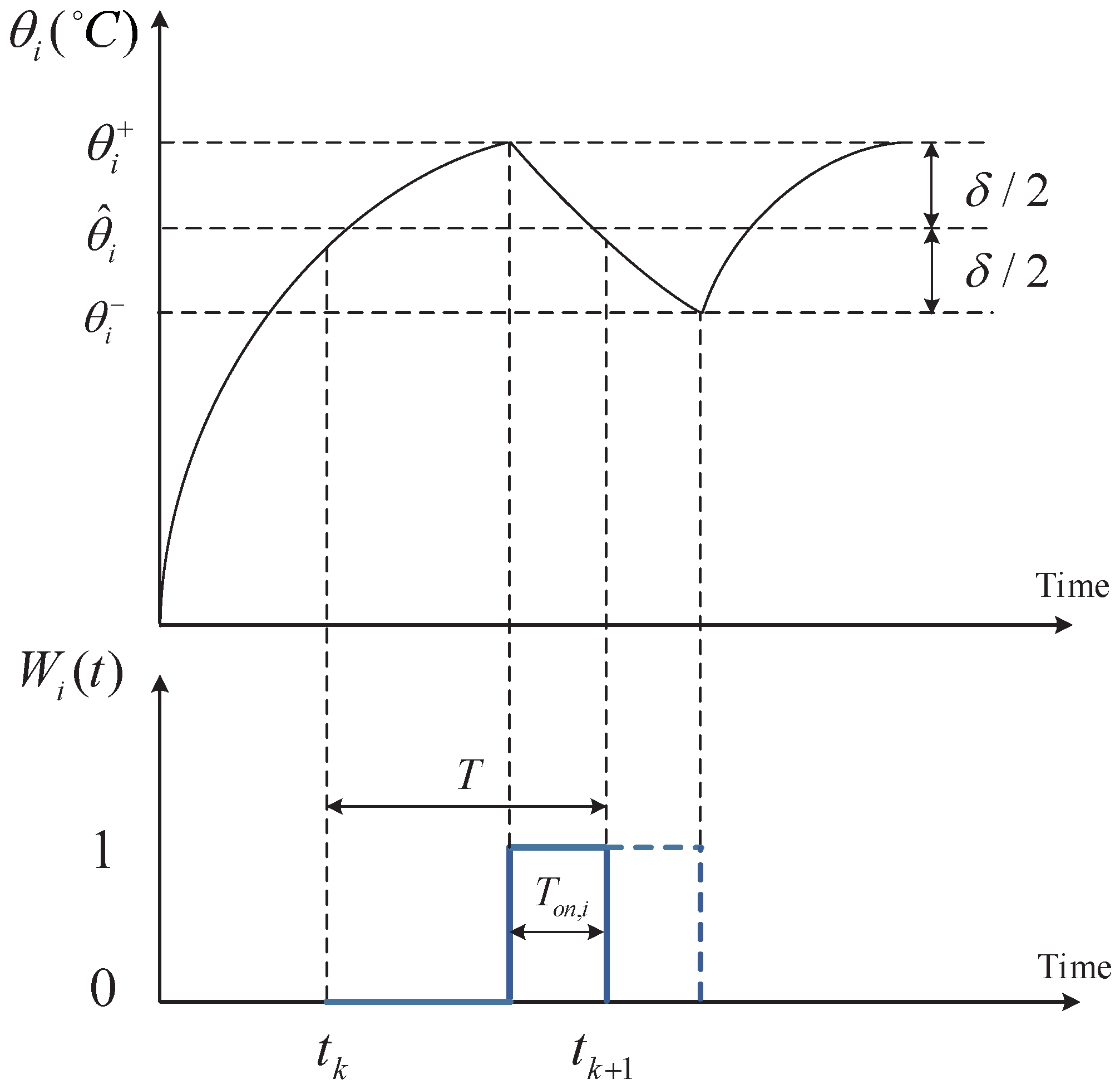
Recall that $T_{on,i}$ is the time length that the “on” state of TCL i lasts during one time horizon $[t_k,t_{k+1}]$, as shown in Figure 2.

Since the maximum value of $T_{on,i}$ is T, the maximum energy demand is ${\beta }_i^{+}\equiv T{P}_i$. Then,

$$0\le u_i\le {\beta }_i^{+}.$$

(5)

The feasible set of $u_i$ is denoted by ${\mathcal{U}}_i$ such that,

$${\mathcal{U}}_i\triangleq \left[0,{\beta }_i^{+}\right],\forall i\in \mathcal{N}.$$

(6)

By (3), $W_i\left(t\right)$ remains unchanged over $\mathcal{T}$ if the internal temperature ${\theta }_i\left(t\right),t\in \mathcal{T}$ always lies in the dead-band. And $W_i\left(t\right)$ changes only if ${\theta }_i\left(t\right)$ hits the limits of the dead-band ${\theta }_i^{-}$ or ${\theta }_i^{+}$ for some $t\in \mathcal{T}$. Then by (1), after the first change of $W_i\left(t\right)$, ${\theta }_i\left(t\right)$ will need some certain time to reach the limit ${\theta }_i^{-}$ or ${\theta }_i^{+}$. Therefore, if given appropriate parameters in (1), ${\theta }_i\left(t\right)$ will not hit the boundary of dead-band twice within $\mathcal{T}$. Then, we have the following assumption in this paper.

Assumption 1.

The switch state $W_i\left(t\right)$ of each TCL i changes no more than once over $\mathcal{T}$.

Based upon Assumption 1, the operation process of TCL i in $\mathcal{T}$ can be divided into two cases w.r.t. $W_i\left(t_k\right)$.

• Case 1 ($W_i\left(t_k\right)=1$): By (1), we have the internal temperature at time $t_k+T_{on,i}$, such that,

  $${\theta }_i(t_k+T_{on,i})=({\theta }_{a,i}\left(t_k\right)-P_i{R}_i)(1-e^{-T_{on,i}/{\tau }_i})+{\theta }_i\left(t_k\right)e^{-T_{on,i}/{\tau }_i}.$$

  (7)
  Combining (2a) and (3), it gives

  $${\theta }_i(t_k+T_{on,i})={\widehat{\theta }}_i-\delta /2.$$

  (8)
  Then by (4), (7) and (8), the relationship between $u_i$ and ${\widehat{\theta }}_i$ is

  $$u_i={\tau }_i{P}_{i}ln\frac{{\theta }_i\left(t_k\right)+P_i{R}_i-{\theta }_{a,i}\left(t_k\right)}{{\widehat{\theta }}_i+P_i{R}_i-{\theta }_{a,i}\left(t_k\right)-\delta /2}.$$

  (9)
• Case 2 ($W_i\left(t_k\right)=0$): Similar with Case 1, by (1)–(4), we have:

  $$u_i=T{P}_i-{\tau }_i{P}_{i}ln\frac{{\theta }_{a,i}\left(t_k\right)-{\theta }_i\left(t_k\right)}{{\theta }_{a,i}\left(t_k\right)-{\widehat{\theta }}_i-\delta /2}.$$

  (10)

In summary, we obtain the relationship between the energy demand $u_i$ and the set-point temperature ${\widehat{\theta }}_i$ such that

$$u_i=f_i\left({\widehat{\theta }}_i\right)=\left\{\begin{array}{c}{\tau }_i{P}_{i}ln\frac{{\theta }_i\left(t_k\right)+P_i{R}_i-{\theta }_{a,i}\left(t_k\right)}{{\widehat{\theta }}_i+P_i{R}_i-{\theta }_{a,i}\left(t_k\right)-\delta /2},\mathrm{in}\mathrm{case}{W}_i\left(t_k\right)=1\hfill \\ T{P}_i-{\tau }_i{P}_{i}ln\frac{{\theta }_{a,i}\left(t_k\right)-{\theta }_i\left(t_k\right)}{{\theta }_{a,i}\left(t_k\right)-{\widehat{\theta }}_i-\delta /2},\mathrm{in}\mathrm{case}{W}_i\left(t_k\right)=0\hfill \end{array}\right.$$

(11)

2.3. Energy Trading Process

As shown in Figure 1, EECC first collects the energy from the wholesale market under the market price $\mathsf{P}$, and then sells the energy to TCL users at a broadcasted price p. Each TCL user adjusts its set-point temperature based on the broadcasted price from EECC. Suppose that EECC and TCL users are strategic players, and all of them make decisions by optimizing their individual objectives. Next we will introduce the preference of EECC and TCL users.

For TCL user $i\in \mathcal{N}$, determining ${\widehat{\theta }}_i$ is equivalent to determining $u_i$ as we have a relationship between them in (11). Hence, TCL user can optimize its energy demand by minimizing its individual cost, which contains the electricity payment and the cost associated with its discomfort level. The individual cost of the i-th TCL user with respect to $u_i$ is given in the following:

$$C_i(u_i;p)\triangleq p{u}_i+\omega d_i\left(u_i\right),$$

(12)

wherein the first term represents the electricity payment and the second is the dissatisfaction cost, and $\omega$ denotes a weighting coefficient concerning the importance of the TCL user’s discomfort during $\mathcal{T}$. For a rational TCL user, its discomfort level continuously decreases with the reduction of the set-point temperature. By (11), the dissatisfaction cost is a function of $u_i$, say $d_i\left(u_i\right)$.

At time $t_k$, before choosing the set-point temperature ${\widehat{\theta }}_i$, each TCL user has a reference temperature, denoted by ${\theta }_i^r$, representing its comfortable temperature. Then, the corresponding reference demand, denoted by $q_i$, can be computed by (11) such that:

$$q_i=\left\{\begin{array}{c}0,\mathrm{in}\mathrm{case}{\theta }_i^r>{\widehat{\theta }}_{i,j}^{+}\hfill \\ f_i\left({\theta }_i^r\right),\mathrm{in}\mathrm{case}{\widehat{\theta }}_{i,j}^{-}\le {\theta }_i^r\le {\widehat{\theta }}_{i,j}^{+}\hfill \\ {\beta }_i^{+},\mathrm{in}\mathrm{case}{\theta }_i^r<{\widehat{\theta }}_{i,j}^{-}\hfill \end{array}\right.$$

(13)

where ${\widehat{\theta }}_{i,j}^{+}$ and ${\widehat{\theta }}_{i,j}^{-}$ represent the i-th TCL user’s maximum and minimum set-point temperature in Case j respectively, with $j=\{1,2\}$.

Remark 3.

In (13), the reference temperature ${\widehat{\theta }}_i^r$ is the threshold value of the comfortable temperature, which is related to each TCL user’s preference and external environment. It can be recognized as a criterion of the comfort level of TCL users.

Remark 4.

By (11), the expression of $f_i({\widehat{\theta }}_i)$ is distinct in different cases. Then, by the feasible set of energy demand in (6), we have ${\widehat{\theta }}_{i,j}^{+}$ and ${\widehat{\theta }}_{i,j}^{-}$ are related to the case j for all $i\in \mathcal{N}$.

As specified in [18,19,20], the dissatisfaction cost function $d_i\left(u_i\right)$ is continuous and has the following properties:

$$\begin{array}{c}\hfill d_i\left(u_i\right)\left\{\begin{array}{c}>0,\mathrm{in}\mathrm{case}{u}_i<q_i\hfill \\ =0,\mathrm{in}\mathrm{case}{u}_i=q_i\hfill \\ <0,\mathrm{in}\mathrm{case}{u}_i>q_i\hfill \end{array}\right.\\ \hfill d_i^{{}^{\prime }}\left(u_i\right)<0,d_i^{{}^{″}}\left(u_i\right)>0\end{array}$$

For $u_i<q_i$, i.e., ${\widehat{\theta }}_i>{\theta }_i^r$, the TCL user is dissatisfied with the current temperature and the discomfort level will increase rapidly as ${\widehat{\theta }}_i$ (demand $u_i$) is away from the reference temperature ${\theta }_i^r$ (demand $q_i$). For $u_i>q_i$, i.e., ${\widehat{\theta }}_i<{\theta }_i^r$, the TCL user is satisfied with the current temperature, but the comfort level will not increase infinitely and change slowly as ${\widehat{\theta }}_i$ is away from the reference temperature ${\theta }_i^r$.

Based on the above properties, we apply the dissatisfaction cost function $d_i\left(u_i\right)$ as the following form [18]:

$$d_i\left(u_i\right)\triangleq e^{b_i(1-u_i/q_i)}-1,$$

(14)

with $b_i>0$, where $b_i$ represents the priority factor of TCL user i.

For EECC, it can obtain benefits by buying energy from the market and selling it to TCL users. Thus as a rational EECC, the selling price should be larger than the market price, i.e., $p\ge \mathsf{P}$. Define the feasible set for the broadcast price p such that

$$\mathcal{P}\triangleq \left\{p|p\ge \mathsf{P}\right\}.$$

(15)

Besides, EECC should consider the discomfort of all the TCL users, otherwise EECC may set the selling price very high to get more benefits. Hence, the utility function of EECC can be expressed as the following form:

$$S_E(p;\mathit{u})\triangleq (p-\mathsf{P})\sum _{i=1}^N{u}_i-\omega \sum _{i=1}^N{d}_i\left(u_i\right),$$

(16)

where $\mathit{u}=[u_1,u_2,\dots ,u_N]$ represents the energy demand of all the TCL users.

3. Stackelberg Game Coordination

As stated in the previous section, EECC buys the total energy that all the TCL users demand from the wholesale market under the market price $\mathsf{P}$ and broadcasts a selling price p to each TCL user. Then, based on the broadcast price p, each TCL user determines the energy demand $u_i$ i.e., setting its set-point temperature ${\widehat{\theta }}_i$.

Note that the decisions between EECC and the TCL users are actually interdependent. We establish a Stackelberg game to describe the interplay of TCL users and EECC in Section 3.1. Furthermore, the existence and uniqueness of the Stackelberg equilibrium are specified in Section 3.2.

3.1. Stackelberg Game

Since there exists a hierarchy among players in Stackelberg games, leaders are in a position to enforce their strategies on the followers. In this leader-follower competition, the followers find the best response function first, i.e., getting to know how they will respond once they observe the strategies of leaders. The leaders are aware of the fact that each follower will choose its best response with respect to the leaders strategies. Hence, the leaders are able to maximize their payoffs anticipating the predicted response of the followers. This is actually observed by the followers to adapt their expected strategy accordingly as a response.

We introduce a one-leader, N-follower Stackelberg game to characterize the electricity transaction process between EECC and TCL users, where EECC serves as the leader and TCL users act as followers. Thus, the system proceeds by the following two stages:

• Stage I: Each TCL user i implements the best response function with respect to the broadcasted price p from EECC.
• Stage II: EECC optimizes the broadcasted price $p^{\ast }$ considering TCL users’ best response ${\mathit{u}}^{\ast }\left(p\right)$ at Stage I.

Then observing EECC’s best strategy, each TCL user i determines its optimal energy demand $u_i^{\ast }$ under the broadcast price $p^{\ast }$ from Stage II. Based on the above set-up, the optimization problem can be formally formulated as the following:

• Leader level:

  $$p^{\ast }=\underset{p\in \mathcal{P}}{arg\; max}{S}_E(p;{\mathit{u}}^{\ast }\left(p\right))$$

  (17)
• Follower level:

  $$u_i^{\ast }\left(p\right)=\underset{u_i\in {\mathcal{U}}_i}{arg\; min}{C}_i(u_i;p)$$

  (18)

The optimal strategies of the game take the form of the Stackelberg equilibrium [30,31]. At the equilibrium, the leader’s strategy $p^{\ast }$ is a solution to the optimization problem specified in (17) based on the best strategy trajectories ${\mathit{u}}^{\ast }\left(p\right)$ of the followers. Each follower’s strategy is also a solution to (18) when it is informed of the equilibrium strategy of the leader. The optimal strategies $u_i^{\ast }\left(p^{\ast }\right),i\in \mathcal{N}$ therefore constitute the equilibrium for all the followers.

Then, we have the following definition of the Stackelberg equilibrium [18,22].

Definition 1 (Stackelberg equilibrium).

The strategy $\left(p^{\ast },{\mathit{u}}^{\ast }\right)$ is a Stackelberg equilibrium if it satisfies:

$$S_E(p^{\ast };{\mathit{u}}^{\ast }\left(p^{\ast }\right))\ge S_E(p;{\mathit{u}}^{\ast }\left(p\right)),$$

(19)

$$C_i(u_i^{\ast };p^{\ast })\le C_i(u_i;p^{\ast }),\mathit{for}\mathit{all}i\in \mathcal{N}.$$

(20)

3.2. Existence and Uniqueness of Stackelberg Equilibrium

Based on the above analysis of the game process, we can deduce the Stackelberg equilibrium by backward induction method [22]. Firstly, each follower determines its best strategy trajectory by solving (18) with respect to a strategy p from the leader. Then, combining the best strategy trajectory ${\mathit{u}}^{\ast }\left(p\right)$ with (17), the leader obtains its best strategy $p^{\ast }$. Subsequently, each follower determines its best strategy $u_i^{\ast }\left(p^{\ast }\right)$ when it is informed of the best strategy $p^{\ast }$ of the leader.

Lemma 1.

Given a broadcast price p from EECC, each follower has a unique optimal strategy $u_i^{\ast }\left(p\right)$, such that:

$$u_i^{\ast }\left(p\right)=\left\{\begin{array}{c}{\beta }_i^{+},\mathit{in}\mathit{case}p\le \frac{w{b}_i}{q_i}{e}^{b_i\left(1-{\beta }_i^{+}/q_i\right)}\hfill \\ q_i-\frac{q_i}{b_i}ln\frac{p{q}_i}{\omega b_i},\mathit{in}\mathit{case}\frac{w{b}_i}{q_i}{e}^{b_i\left(1-{\beta }_i^{+}/q_i\right)}<p<\frac{w{b}_i}{q_i}{e}^{b_i}\hfill \\ 0,\mathit{in}\mathit{case}p\ge \frac{w{b}_i}{q_i}{e}^{b_i}\hfill \end{array}\right.$$

Proof of Lemma 1.

By (12) and (14), we obtain that each follower’s utility function $C_i(u_i;p)$ is continuous and differentiable over a convex set ${\mathcal{U}}_i$.

Then, by (12), we have

$$\begin{array}{c}\hfill {\partial }^2{C}_i(u_i;p)/\partial u_i^2=\frac{\omega b_i^2}{q_i^2}{e}^{b_i(1-u_i/q_i)}>0.\end{array}$$

Hence, $C_i(u_i;p)$ is a strictly convex function w.r.t. $u_i$.

By $\partial C_i(u_i;p)/\partial u_i=0$, we obtain the optimal trajectory w.r.t p as below:

$${\tilde{u}}_i\left(p\right)=q_i-\frac{q_i}{b_i}ln\frac{p{q}_i}{\omega b_i}.$$

(21)

Furthermore, because the feasible set ${\mathcal{U}}_i$ defined in (6) is a bounded set, the boundary conditions of the optimal strategy in (21) is determined by (21). ☐

Based on the best strategies ${\mathit{u}}^{\ast }\left(p\right)$, EECC determines the best electricity prices $p^{\ast }$ by maximizing its utility function (16).

Lemma 2.

The leader has a unique optimal strategy $p^{\ast }$, such that:

$$\begin{array}{c}\hfill p^{\ast }=\underset{p\in \left[\mathsf{P},p_{max}\right)}{arg\; max}{S}_E\left(p;{\mathit{u}}^{\ast }\left(p\right)\right),\end{array}$$

(22)

where $p_{max}\equiv {max}_{i\in \mathcal{N}}\left\{\frac{\omega b_i}{q_i}{e}^{b_i}\right\}$.

Proof of Lemma 2.

The Proof of Lemma 2 is given in Appendix A. ☐

Remark 5.

From Lemma 2, there exists a unique optimal strategy (22) when $p\in \left[\mathsf{P},p_{max}\right)$. Considering $p\ge p_{max}$, we have $u_i^{\ast }\left(p\right)=0$ by (21), for all $i\in \mathcal{N}$. In addition, by (16), we obtain that the utility function $S_E(p;u_i^{\ast }\left(p\right))=-\omega {\sum }_{i=1}^N{d}_i\left(0\right)$ is a constant for all $p\ge p_{max}$. Therefore, there is no unique optimal strategy in the given range of p.

Theorem 1.

Considering $p_{max}>\mathsf{P}$, there exists a unique Stackelberg equilibrium $\left(p^{\ast },{\mathit{u}}^{\ast }\right)$ for the proposed game.

Proof of Theorem 2.

By Lemma 1, we have $C_i(u_i^{\ast };p^{\ast })\le C_i(u_i;p^{\ast })$ for all $i\in \mathcal{N}$, then (20) holds. Then, by Lemma 2, (19) is satisfied. Therefore, according to the Definition 1, $\left(p^{\ast },{\mathit{u}}^{\ast }\right)$ is the unique equilibrium of the Stackelberg game.

Remark 6.

If $p_{max}\le \mathsf{P}$, then we have EECC’s utility function $S_E(p;u_i^{\ast }\left(p\right))=-\omega {\sum }_{i=1}^N{d}_i\left(0\right)$. Thus, considering $p_{max}\le \mathsf{P}$, EECC cannot find a unique optimal strategy.

Based upon Theorem 1, we specify Algorithm 1 to achieve the Stackelberg equilibrium of the game.

Algorithm 1 DR algorithm by Backward Induction.

Require: Initialize the time horizon $\mathcal{T}\equiv [t_k,t_k+T]$; Initialize the switch state $W_i\left(t_k\right)$ of TCL user i; Initialize the market price $\mathsf{P}$; Initialize the reference temperature ${\theta }_i^r$ of TCL user i; Set the reference demand $q_i$ of TCL user i by (13) w.r.t ${\theta }_i^r$. Ensure: EECC’s optimal broadcast price $p^{\ast }$; Each TCL user’s adjusted set-point temperature ${\widehat{\theta }}_i^{\ast }$.   1: By (22), EECC determines the optimal broadcast price $p^{\ast }$ w.r.t the best strategy trajectory $u_i^{\ast }\left(p\right)$ in (21); 2: Each TCL user $i\in \mathcal{N}$ determines the optimal strategy $u_i^{\ast }$ w.r.t. $p^{\ast }$ by (21); 3: Each TCL user $i\in \mathcal{N}$ computes their optimal set-point temperature ${\widehat{\theta }}_i^{\ast }$ by ${\widehat{\theta }}_i^{\ast }=f_i^{(-1)}\left(u_i^{\ast }\right)$.

As stated in [18,19], compared with other methods which usually involve interactive iteration processes between the leader and the followers, which are EECC and the TCL users respectively in the underlying games, the DR algorithm based on Backward Induction proposed in our work can significantly reduce the computational time in implementing the equilibrium of the underlying Stackelberg games.

4. Simulation

In this part, some case studies are analyzed to demonstrate the price response coordination of TCLs. The proposed Stackelberg game model and control scheme are validated by the simulations in MATLAB 2014a. Besides, we use the interior-point method to solve the optimization problems and the computational time of all cases are limited in $2.0$ s.

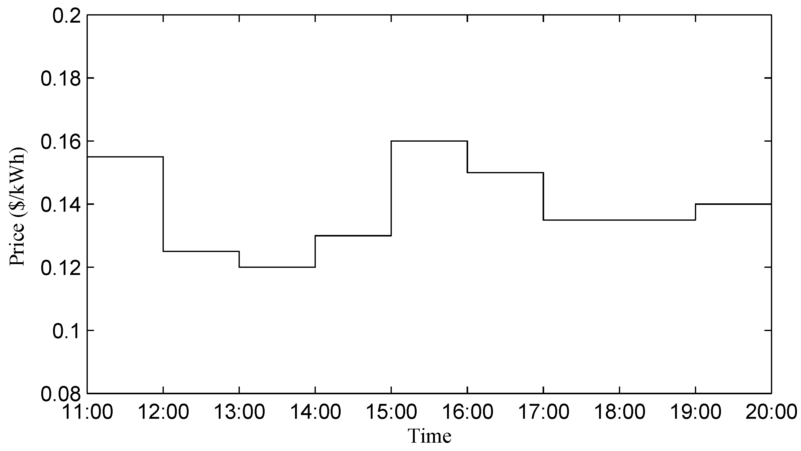
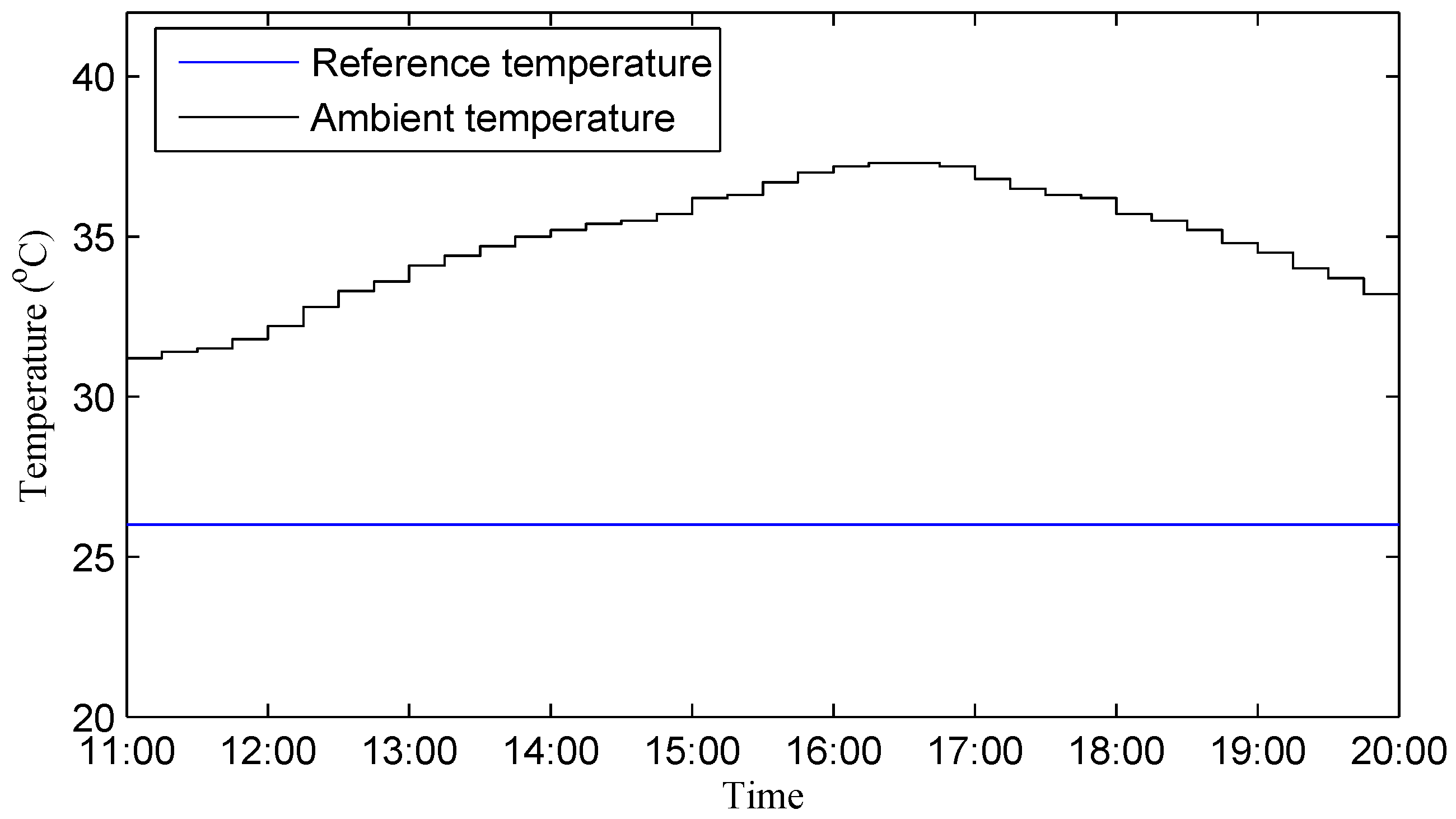
We adopt a typical 15-min based pricing by dividing 9-h into 36 equal time instants [19], as shown in Figure 3. An ambient temperature profile from 11:00 to 20:00 in a typical summer day is shown in Figure 4.

4.1. Homogeneous Case

We first consider $N=100$ homogeneous TCLs, and the parameters of the TCLs are specified in

Table 2. TCL parameters.

Parameter	Homogeneous TCL	Heterogeneous TCL
R	$2{}^{\circ }\mathrm{C}$/kW	$2{}^{\circ }\mathrm{C}$/kW
C	5 kWh/${}^{\circ }\mathrm{C}$	6 kWh/${}^{\circ }\mathrm{C}$
P	11 kW	14 kW
${\beta }^{+}$	2.75 kWh	3.5 kWh
b	1.1	1.5

[32]. We set the weighting factor of the importance of the discomfort level as $\omega =0.2$.

Without loss of generality, assume that $W_i\left(t_k\right)=0$ with $t_k=11:00$, for all $i\in \mathcal{N}$, i.e., the switch state of each TCL is “off” at 11:00. As specified in Section 2.2, the “off” state implies that $j=2$.

We also consider the internal temperature ${\theta }_i\left(t_k\right)=27{}^{\circ }\mathrm{C}$ for all $i\in \mathcal{N}$ and the temperature dead-band $\delta =0.25{}^{\circ }\mathrm{C}$.

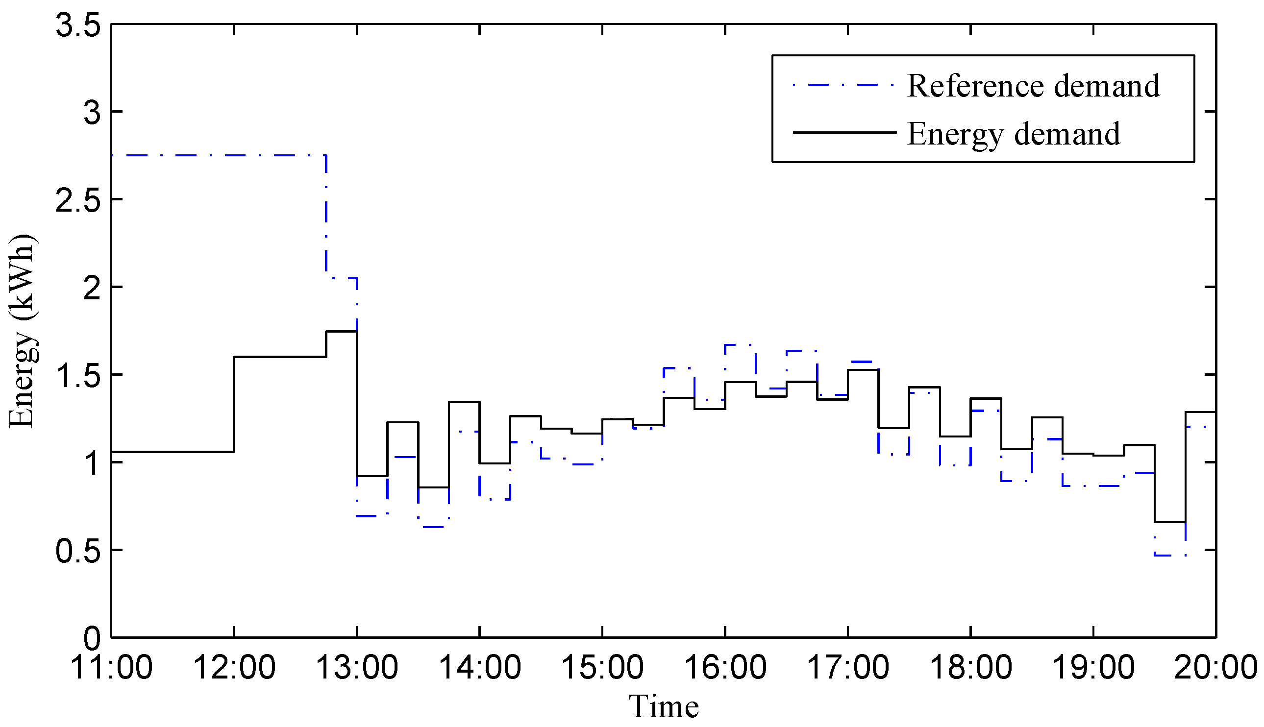
Then, according to the reference temperature ${\theta }_i^r$ of TCL user i shown in Figure 4, we obtain the reference demand energy $q_i$ by (13), which is displayed by the blue dash-dot line in Figure 5. More specifically, taking one time horizon [11:00, 11:15] as an example and given ${\theta }_{a,i}\left(t_k\right)=31.2{}^{\circ }\mathrm{C}$, ${\theta }_i\left(t_k\right)=27{}^{\circ }\mathrm{C}$ and ${\theta }_i^r\left(t_k\right)=26{}^{\circ }\mathrm{C}$, we calculate that ${\widehat{\theta }}_i^{-}=f_i^{(-1)}\left({\beta }_i^{+}\right)=26.56{}^{\circ }\mathrm{C}$ in Case 2. Then by (13), we have $q_i\left(t_k\right)={\beta }_i^{+}=2.275$kWh.

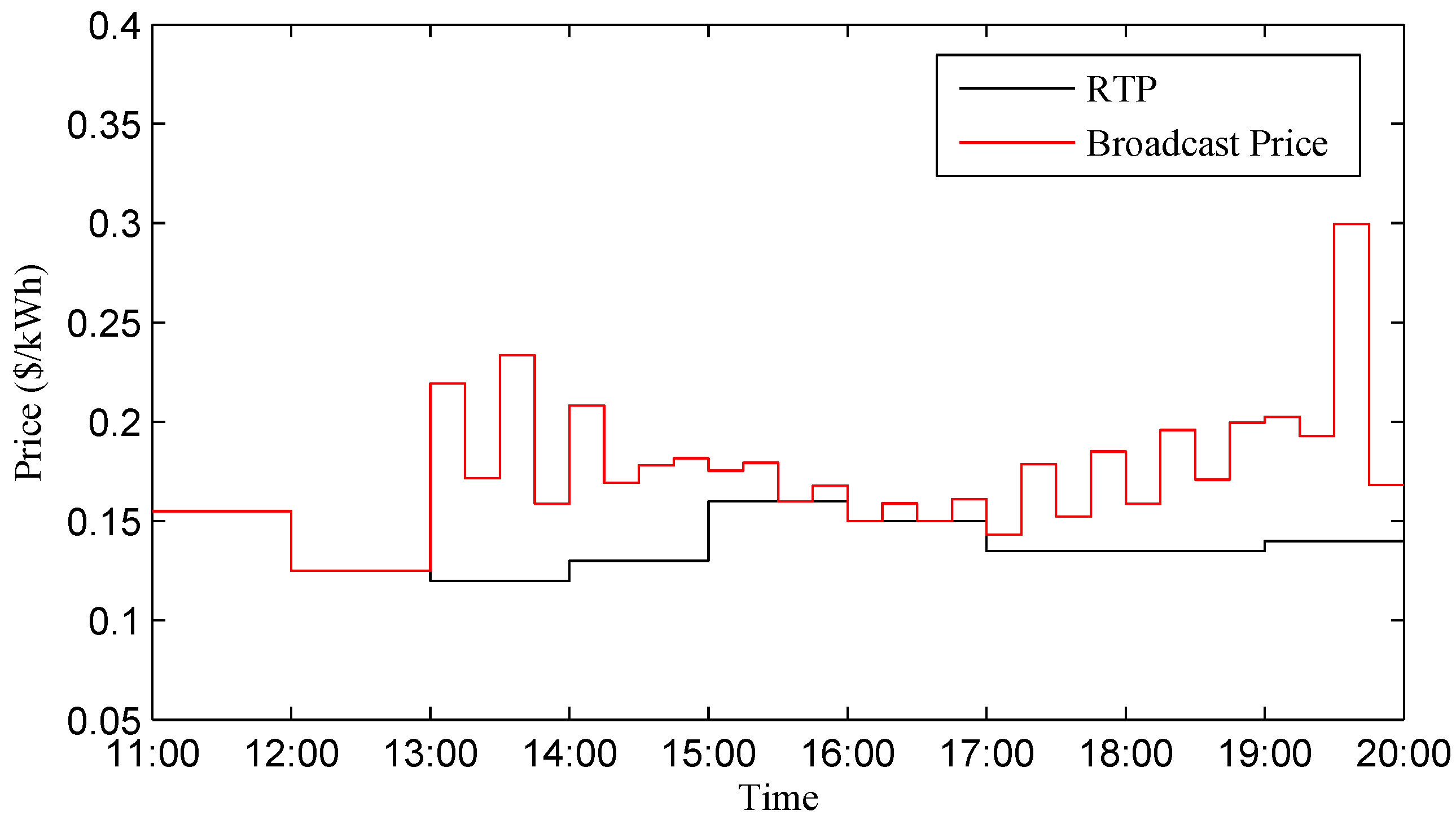
By applying Algorithm 1, EECC implements the optimal price $p^{\ast }$ w.r.t ${\mathit{u}}^{\ast }\left(p\right)$ by (22), which is displayed by the red line in Figure 6.

The broadcast price $p^{\ast }$ satisfies $p^{\ast }\in \left(\frac{\omega b_i}{q_i}{e}^{(1-{\beta }_i^{+}/q_i)},\frac{\omega b_i}{q_i}{e}_i^b\right)$. Then, by (21), the optimal energy demand of each TCL user $u_i^{\ast }$ increases as $p^{\ast }$ decreases from 11:00 to 20:00, which is displayed in Figure 5.

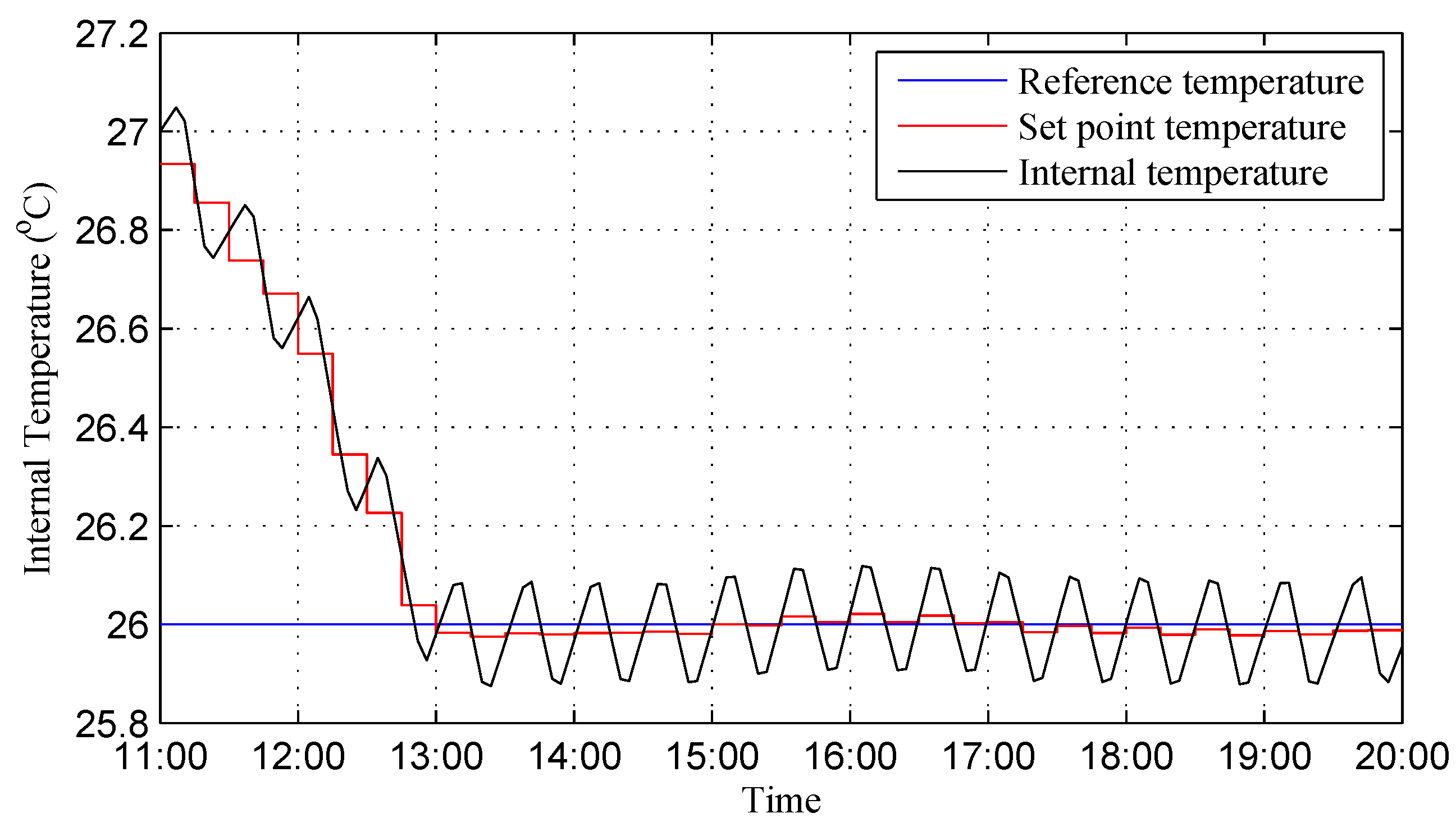
Subsequently, according to the relationship between the set-point temperature and the energy demand specified in Section 2.2, each TCL user adjusts its set-point temperature by ${\widehat{\theta }}_i^{\ast }=f_i^{(-1)}\left(u_i^{\ast }\right)$, which is displayed by the red line in Figure 7.

Consider the time horizon [13:00, 13:15] as an example. Based upon the reference demand $q_i=0.691$kWh, the market price $\mathsf{P}=0.12$$/kWh and the optimal reaction curve $u_i^{\ast }\left(p\right)=q_i-\frac{q_i}{b_i}ln\frac{p{q}_i}{\omega b_i}$ given in Lemma 1, we obtain the optimal broadcast price $p^{\ast }=0.219$ $/kWh by (22). Afterwards, TCL users observe the best strategy of EECC and compute their best strategies ${\mathit{u}}_i^{\ast }\left(p^{\ast }\right)$ by (21). The corresponding set-point temperature is ${\widehat{\theta }}_i^{\ast }=25.98{}^{\circ }\mathrm{C}$. Because of the existence of the dead-band $\delta$, the internal temperature varies by (1) in [13:00, 13:15], and the switch state will change when the internal temperature hits the upper limit ${\widehat{\theta }}_i^{\ast }+\delta /2=26.11{}^{\circ }\mathrm{C}$.

Moreover, after 13:00, for keeping the internal temperature around the reference temperature $26{}^{\circ }\mathrm{C}$, the switch state changes one time within each time horizon and the optimal set-point temperature stays around $26{}^{\circ }\mathrm{C}$, as illustrated in Figure 7. However, given the same ambient temperature ${\widehat{\theta }}_{a,i}$, by (9) and (10), the associate reference energy demand $q_i$ are distinct in different cases. This causes the fluctuation of the energy demand trajectory as displayed in Figure 5.

4.2. Heterogeneous Case

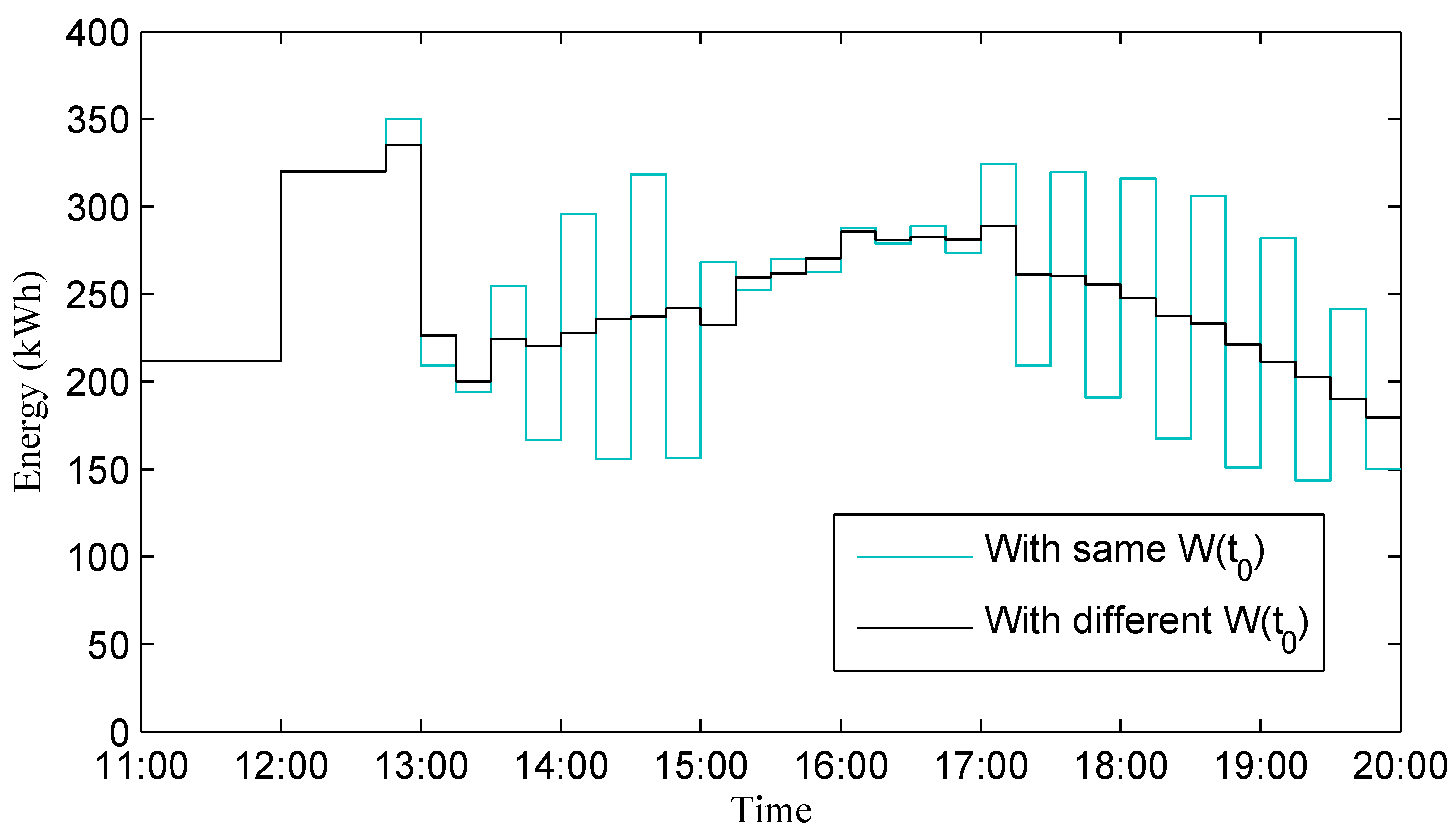
In general, the aggregated TCLs’ switch state are different [14]. For the purpose of demonstration, we suppose that the total 100 TCLs are partitioned into two categories, say 50 TCLs are with $W_i\left(t_k\right)=1$ and another 50 TCLs with $W_i\left(t_k\right)=0$. As a sequence, the profile of the aggregated energy demand of the 100 TCLs is displayed by the black line in Figure 8.

As observed in Figure 8, the fluctuations of individual TCLs are alleviated by the aggregated TCLs with different $W_i\left(t_k\right)$. Thus, we may induce the TCL users to adjust its set-point temperature, to mitigate the fluctuation of the power grid by broadcasting different prices to the groups of TCL1 and TCL2 respectively.

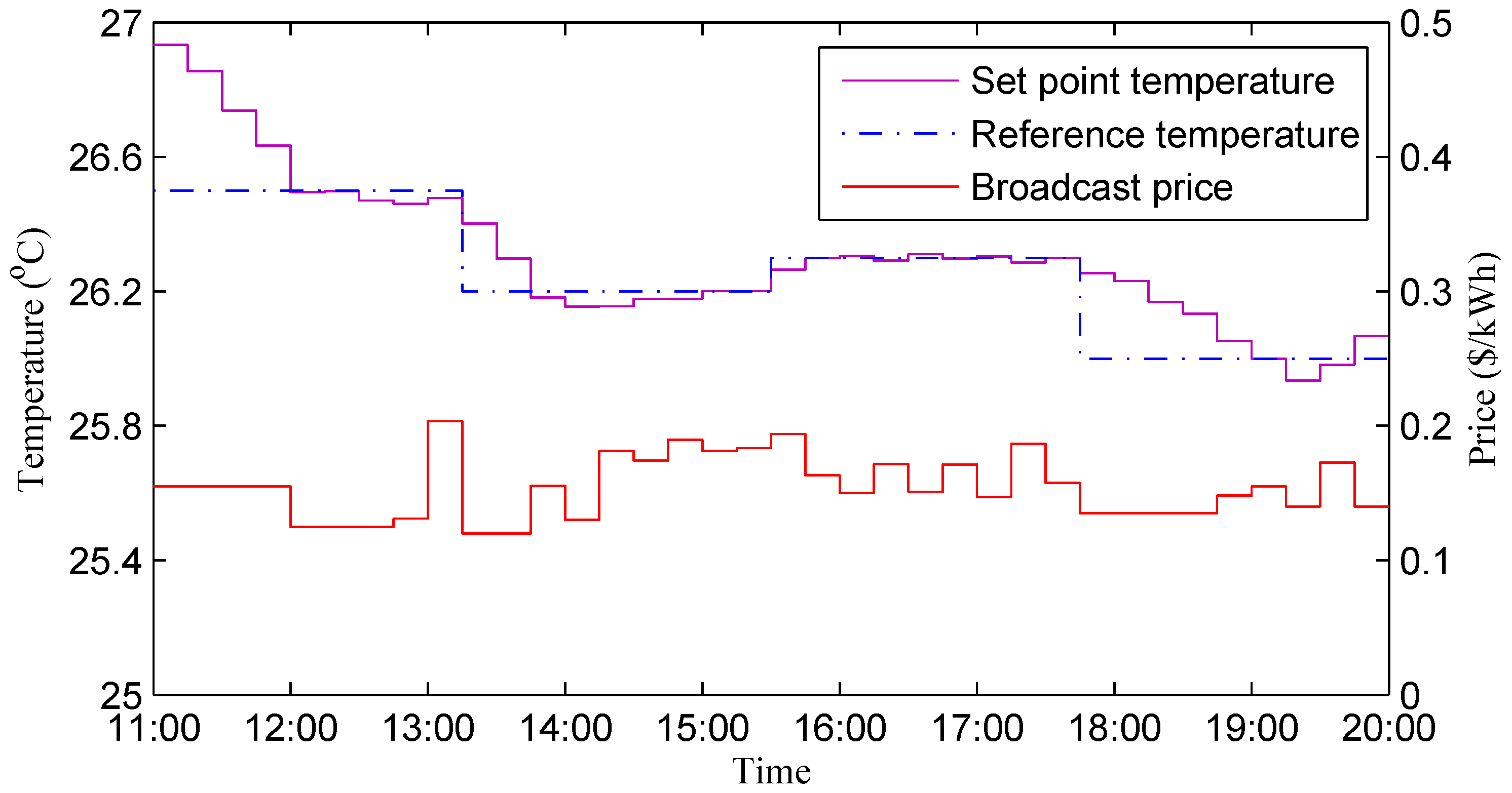
Furthermore, because of the different characteristics of the TCL users, the reference temperature will change with respect to the variational external environment, such as the ambient temperature and the human actions in the room. Therefore, in Figure 9, we consider a scenario with variational reference temperature. EECC broadcasts price $p^{\ast }$ (displayed by the red line) and TCL user i implements the set-point temperature ${\widehat{\theta }}_i^{\ast }$ accordingly (displayed by the purple line) at each instant to maximize the utility benefit and minimize the individual cost of each TCL user.

In reality, the TCLs’ properties vary according to the different preferences of TCL users. Thus, besides the above study for homogeneous TCLs, here we also apply Algorithm 1 for the heterogeneous cases.

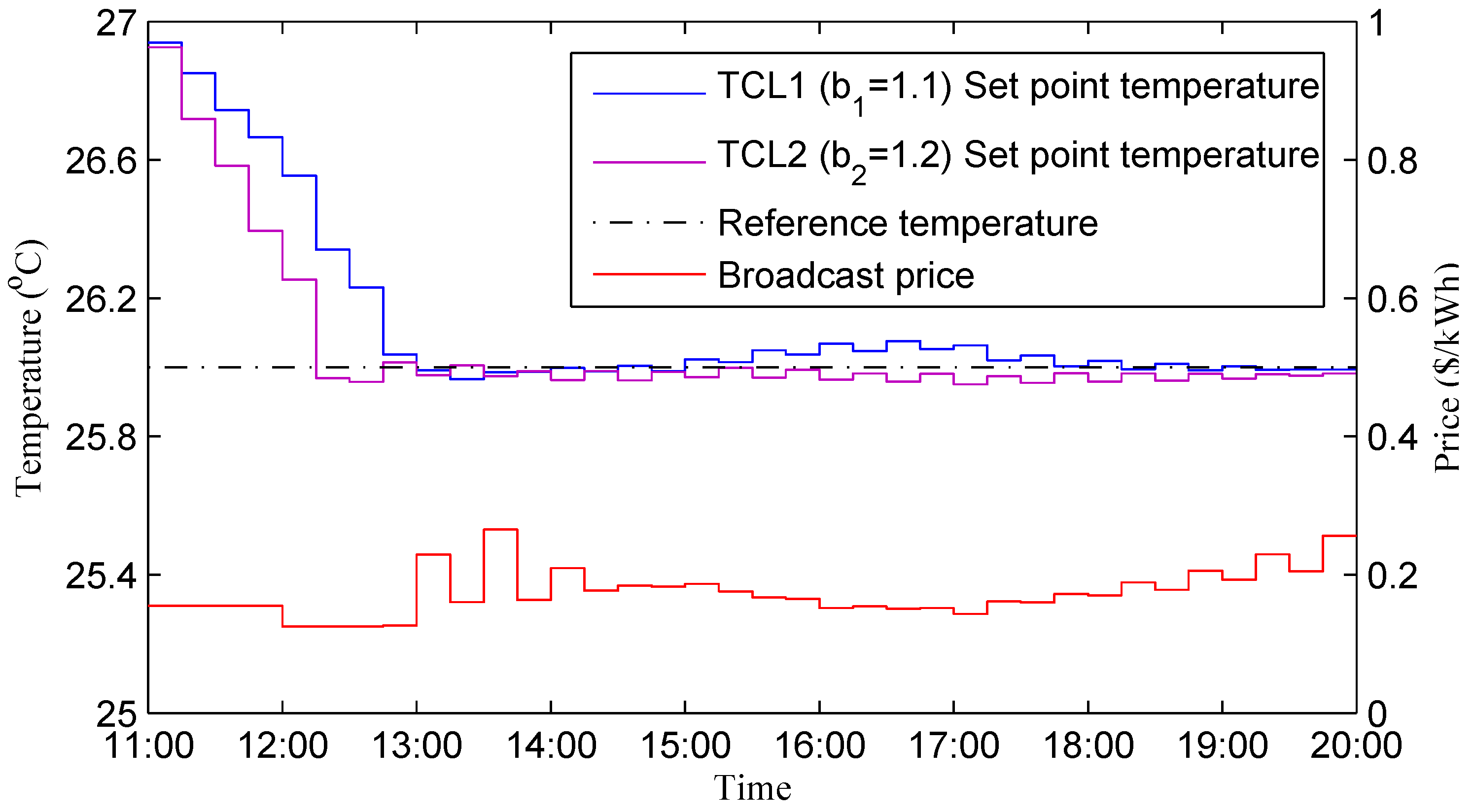
We first consider different priority factors of TCL users. By (14), we obtain that the TCL user with higher b will have more discomfort when the set-point temperature exceeds the reference temperature. Therefore, the set-point temperature of TCL2 with $b_2=1.2$ decreases faster than TCL1 with $b_1=1.1$, which is displayed in Figure 10.

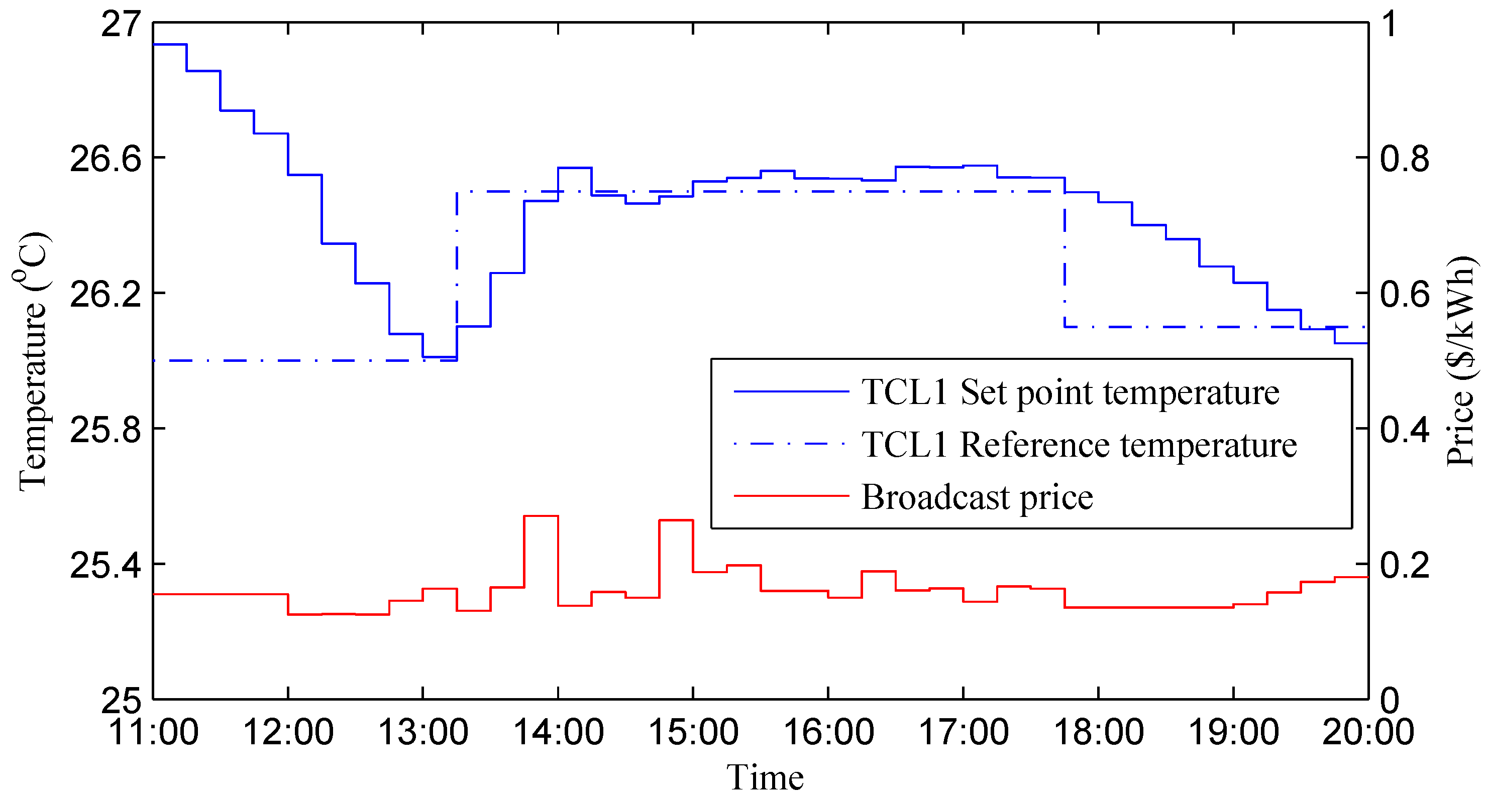
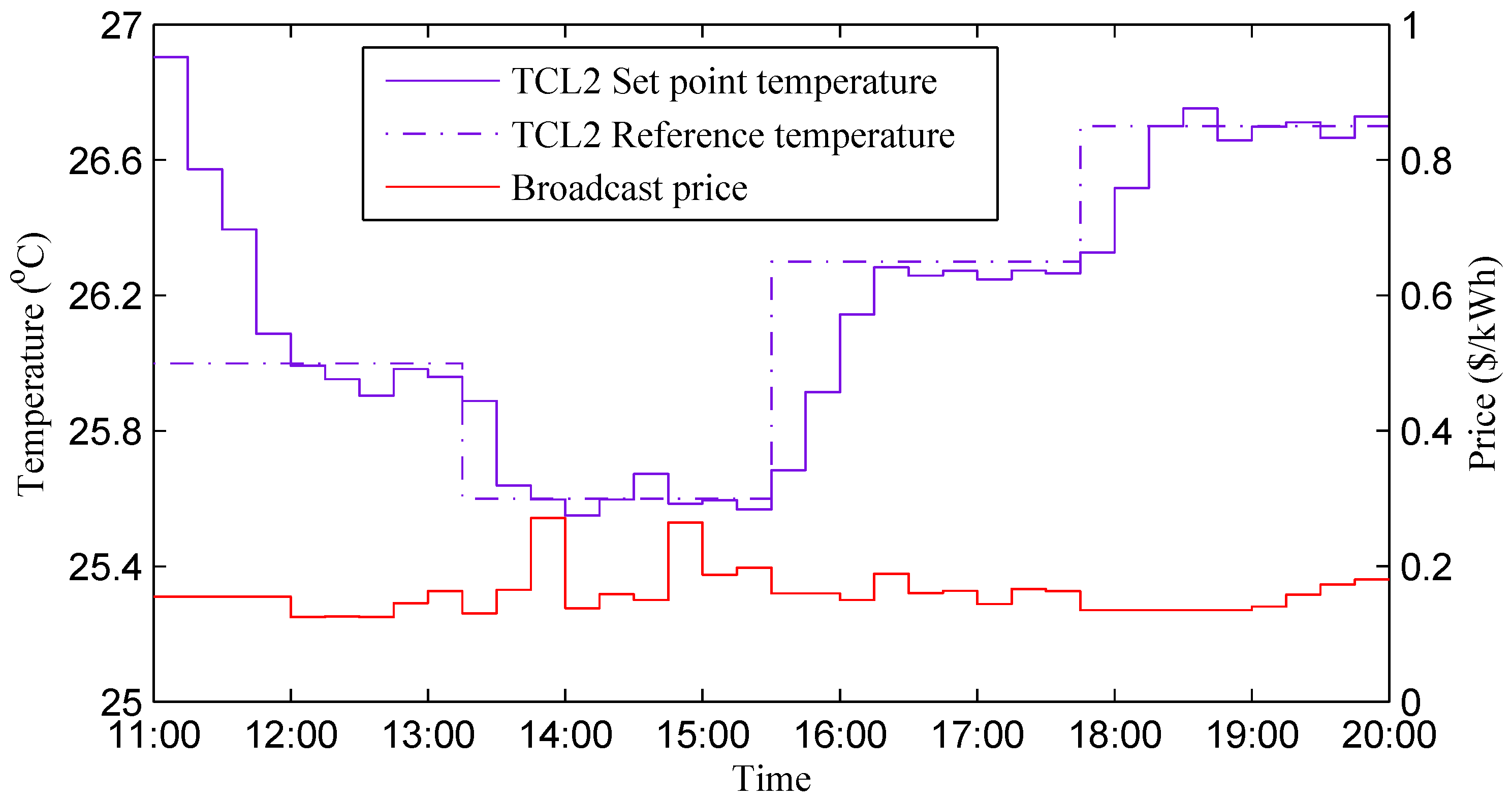
Furthermore, we consider the heterogeneous case with variational reference temperature and different properties of TCLs. The parameters of heterogeneous TCLs are shown in Table 2. Figure 11 and Figure 12 display the best broadcast price from EECC and the set-point temperature of different TCLs respectively.

5. Conclusions and Ongoing Reasearch

We have studied the coordination of TCLs under a Stackelberg game based price response scheme. Based upon the dynamics of the TCLs, we first establish the relationship between the set-point temperature and the energy consumed to reach the set-point temperature. Then, a discomfort function is defined to represent the discomfort level of the set-point temperature. Based upon the interplay of TCL users and EECC during the electricity trading process, a one-leader N-follower Stackelberg game is established. EECC optimizes its selling price considering the tradeoff of its electricity gross benefit and the dissatisfaction cost of TCL users, while TCL users make decisions by minimizing the electricity payments and the dissatisfaction cost. Compared with other iteration methods in the literature, a more effective DR algorithm by backward induction method is proposed to achieve the unique Stackelberg equilibrium. At the equilibrium, EECC maximizes its utility function and each TCL user adjusts its set-point temperature to minimize its cost.

In the future, unlike the model considered in the current work, we will extend our work by considering the heat exchanges among the TCLs which are interactive with each other. Besides, we would like to design a different electricity price scheme to satisfy different users’ preferences and maximize the utility benefits.

References

- Siano, P. Demand response and smart grids—A survey. Renew. Sustain. Energy Rev. 2014, 30, 461–478. [Google Scholar] [CrossRef]
- Meng, F.L.; Zeng, X.J. An optimal real-time pricing for demand-side management: A Stackelberg game and genetic algorithm approach. In Proceedings of the 2014 International Joint Conference on Neural Networks, Beijing, China, 6–11 July 2014; pp. 1703–1710. [Google Scholar]
- Ipakchi, A.; Albuyeh, F. Grid of the future. IEEE Power Energy Mag. 2009, 7, 52–62. [Google Scholar] [CrossRef]
- Molderink, A.; Bakker, V.; Bosman, M.G.C.; Hurink, J.L.; Smit, G.J.M. Management and Control of Domestic Smart Grid Technology. IEEE Trans. Smart Grid 2010, 1, 109–119. [Google Scholar] [CrossRef] [Green Version]
- Callaway, D.S. Tapping the energy storage potential in electric loads to deliver load following and regulation, with application to wind energy. Energy Convers. Manag. 2009, 50, 1389–1400. [Google Scholar] [CrossRef]
- He, H.; Sanandaji, B.M.; Poolla, K.; Vincent, T.L. Aggregate Flexibility of Thermostatically Controlled Loads. IEEE Trans. Power Syst. 2013, 30, 189–198. [Google Scholar]
- Borenstein, S. The Long-Run Efficiency of Real-Time Electricity Pricing. Energy J. 2005, 26, 93–116. [Google Scholar] [CrossRef]
- Maharjan, S.; Zhu, Q.; Zhang, Y.; Gjessing, S.; Başar, T. Demand Response Management in the Smart Grid in a Large Population Regime. IEEE Trans. Smart Grid 2015, 7, 189–199. [Google Scholar] [CrossRef]
- Yu, M.; Hong, S.H. Supply-demand balancing for power management in smart grid: A Stackelberg game approach. Appl. Energy 2016, 164, 702–710. [Google Scholar] [CrossRef]
- Ma, Z.; Zou, S.; Ran, L.; Shi, X.; Hiskens, I.A. Efficient decentralized coordination of large-scale plug-in electric vehicle charging. Automatica 2016, 69, 35–47. [Google Scholar] [CrossRef]
- Dai, Y.; Gao, Y.; Gao, H.; Zhu, H. Real-time pricing scheme based on Stackelberg game in smart grid with multiple power retailers. Neurocomputing 2017, 260, 149–156. [Google Scholar] [CrossRef]
- Mortensen, R.E.; Haggerty, K.P. A stochastic computer model for heating and cooling loads. IEEE Trans. Power Syst. 1988, 3, 1213–1219. [Google Scholar] [CrossRef]
- Ucak, C.; Caglar, R. The effects of load parameter dispersion and direct load control actions on aggregated load. In Proceedings of the 1998 International Conference on Power System Technology, Beijing, China, 18–21 August 1998; Volume 1, pp. 280–284. [Google Scholar]
- Bashash, S.; Fathy, H.K. Modeling and Control of Aggregate Air Conditioning Loads for Robust Renewable Power Management. IEEE Trans. Control Syst. Technol. 2013, 21, 1318–1327. [Google Scholar] [CrossRef]
- Koch, S.; Mathieu, J.L.; Callaway, D.S. Modeling and control of aggregated heterogeneous thermostatically controlled loads for ancillary services. In Proceedings of the Power Systems Computation Conference, Stockholm, Sweden, 22–26 August 2011. [Google Scholar]
- Ghanavati, M.; Chakravarthy, A. Demand-Side Energy Management by Use of a Design-Then-Approximate Controller for Aggregated Thermostatic Loads. IEEE Trans. Control Syst. Technol. 2017, 26, 1439–1448. [Google Scholar] [CrossRef]
- Mathieu, J.L.; Koch, S.; Callaway, D.S. State Estimation and Control of Electric Loads to Manage Real-Time Energy Imbalance. IEEE Trans. Power Syst. 2013, 28, 430–440. [Google Scholar] [CrossRef]
- Yu, M.; Hong, S.H. A Real-Time Demand-Response Algorithm for Smart Grids: A Stackelberg Game Approach. IEEE Trans. Smart Grid 2017, 7, 879–888. [Google Scholar] [CrossRef]
- Yang, P.; Tang, G.; Nehorai, A. A game-theoretic approach for optimal time-of-use electricity pricing. IEEE Trans. Power Syst. 2013, 28, 884–892. [Google Scholar] [CrossRef]
- Samadi, P.; Mohsenian-Rad, A.H.; Schober, R.; Wong, V.W.S.; Jatskevich, J. Optimal Real-Time Pricing Algorithm Based on Utility Maximization for Smart Grid. In Proceedings of the IEEE International Conference on Smart Grid Communications, Gaithersburg, MD, USA, 4–6 October 2010; pp. 415–420. [Google Scholar]
- Tushar, W.; Chai, B.; Yuen, C.; Smith, D.B. Three-Party Energy Management With Distributed Energy Resources in Smart Grid. IEEE Trans. Ind. Electron. 2015, 62, 2487–2498. [Google Scholar] [CrossRef] [Green Version]
- Osborne, M.J.; Rubinstein, A. A Course in Game Theory; MIT Press: Cambridge, MA, USA, 1994. [Google Scholar]
- Ladurantaye, D.D.; Gendreau, M.; Potvin, J.Y. Strategic Bidding for Price-Taker Hydroelectricity Producers. IEEE Trans. Power Syst. 2007, 22, 2187–2203. [Google Scholar] [CrossRef]
- Conejo, A.J.; Nogales, F.J.; Arroyo, J.M. Price-Taker Bidding Strategy under Price Uncertainty. IEEE Power Eng. Rev. 2002, 22, 57. [Google Scholar] [CrossRef]
- Liu, M.; Shi, Y. Model Predictive Control for Thermostatically Controlled Appliances Providing Balancing Service. IEEE Trans. Control Syst. Technol. 2016, 24, 2082–2093. [Google Scholar] [CrossRef]
- Barata, F.A.; Igreja, J.M.; Rui, N.S. Demand Side Management Energy Management System for Distributed Networks; Springer International Publishing: Basel, Switzerland, 2016; pp. 455–471. [Google Scholar]
- Perfumo, C.; Braslavsky, J.H.; Ward, J.K. Model-Based Estimation of Energy Savings in Load Control Events for Thermostatically Controlled Loads. IEEE Trans. Smart Grid 2014, 5, 1410–1420. [Google Scholar] [CrossRef]
- Yong, T.Y.; Jin, Y.G. Methods for Adding Demand Response Capability to a Thermostatically Controlled Load with an Existing On-off Controller. J. Electr. Eng. Technol. 2015, 10, 755–765. [Google Scholar] [Green Version]
- Tsui, K.M.; Chan, S.C. Demand Response Optimization for Smart Home Scheduling Under Real-Time Pricing. IEEE Trans. Smart Grid 2012, 3, 1812–1821. [Google Scholar] [CrossRef]
- Meng, F.L.; Zeng, X.J. A Stackelberg game-theoretic approach to optimal real-time pricing for the smart grid. Soft Comput. 2013, 17, 2365–2380. [Google Scholar] [CrossRef]
- Maharjan, S.; Zhu, Q.; Zhang, Y.; Gjessing, S.; Basar, T. Dependable Demand Response Management in the Smart Grid: A Stackelberg Game Approach. IEEE Trans. Smart Grid 2013, 4, 120–132. [Google Scholar] [CrossRef]
- Mathieu, J.L.; Callaway, D.S. State Estimation and Control of Heterogeneous Thermostatically Controlled Loads for Load Following. In Proceedings of the Hawaii International Conference on System Science, Maui, HI, USA, 4–7 January 2012; pp. 2002–2011. [Google Scholar]
Figure 1.
The framework of the energy trading process.
Figure 2.
Temperature evolution procedure of thermostatically controlled loads (TCLs).
Figure 3.
Market price data.
Figure 4.
Ambient temperature and Reference temperature from 11:00 to 20:00 on a summer day.
Figure 5.
Optimal energy demand of the TCL.
Figure 6.
Broadcast price from electric energy control center (EECC).
Figure 7.
Set-point temperature and Internal temperature of the TCLs.
Figure 8.
One hundred TCLs with the same vs. 100 TCLs with different .
Figure 9.
Variational reference temperature.
Figure 10.
TCLs with different priority factor b.
Figure 11.
Heterogeneous TCLs: set-point temperature of TCL1.
Figure 12.
Heterogeneous TCLs: set-point temperature of TCL2.