Feature Selection and Transfer Learning for Alzheimer’s Disease Clinical Diagnosis


1
School of Information Engineering, Guangdong Medical University, Zhanjiang 524023, China
2
School of Software, South China University of Technology, Guangzhou 510006, China
*
Author to whom correspondence should be addressed.
Appl. Sci. 2018, 8(8), 1372; https://doi.org/10.3390/app8081372
Submission received: 25 July 2018
/
Revised: 10 August 2018
/
Accepted: 11 August 2018
/
Published: 15 August 2018
(This article belongs to the Section Applied Biosciences and Bioengineering)
Abstract
:Background and Purpose: A majority studies on diagnosis of Alzheimer’s Disease (AD) are based on an assumption: the training and testing data are drawn from the same distribution. However, in the diagnosis of AD and mild cognitive impairment (MCI), this identical-distribution assumption may not hold. To solve this problem, we utilize the transfer learning method into the diagnosis of AD. Methods: The MR (Magnetic Resonance) images were segmented using spm-Dartel toolbox and registrated with Automatic Anatomical Labeling (AAL) atlas, then the gray matter (GM) tissue volume of the anatomical region were computed as characteristic parameter. The information gain was introduced for feature selection. The TrAdaboost algorithm was used to classify AD, MCI, and normal controls (NC) data from Alzheimer’s Disease Neuroimaging Initiative (ADNI) database, meanwhile, the “knowledge” learned from ADNI was transferred to AD samples from local hospital. The classification accuracy, sensitivity and specificity were calculated and compared with four classical algorithms. Results: In the experiment of transfer task: AD to MCI, 177 AD and 40NC subjects were grouped as training data; 245 MCI and 45 remaining NC subjects were combined as testing data, the highest accuracy achieved 85.4%, higher than the other four classical algorithms. Meanwhile, feature selection that is based on information gain reduced the features from 90 to 7, controlled the redundancy efficiently. In the experiment of transfer task: ADNI to local hospital data, the highest accuracy achieved 93.7%, and the specificity achieved 100%. Conclusions: The experimental results showed that our algorithm has a clear advantage over classic classification methods with higher accuracy and less fluctuation.
1. Introduction
Alzheimer’s Disease (AD) is the most prevalent neurodegenerative dementia worldwide. It is reported that the number of affected patients is expected to double in the next 20 years, and one in 85 people will be affected by 2050. Thus, the early accurate diagnosis of AD is crucial, as an intermediate stage between normal age-related cognitive decline and dementia, mild cognitive impairment (MCI) has been identified [1]. It may provide a window of chance for treatment and intervention before the disease advances. However, MCI does not always lead to AD and the MCI group is very heterogeneous. It is a highly relevant task to differentiate MCI subjects who have greater risk of developing AD within the next few years from those who will remain stable or even improve [2]. Thus, it is of great interest to identify MCI and also to predict its risk of progressing to AD.
Accumulated evidence demonstrates that individuals with AD have both functional and structural changes in their brains, such as loss of gray matter volume [3]. However, these findings are mainly obtained based on group-level statistical comparison, and are thus of limited value for individual-based disease diagnosis. Therefore, some recent studies tried to solve this problem by using magnetic resonance imaging (MRI) and algorithms from machine learning [4,5]. Computer-based decision shows its efficiency in the detection of the early stage diseases.
Recently, many machine learning classification methods have been used for the early diagnosis of AD, including the structural brain atrophy measured by MRI [6,7,8]. Data mining approaches, such as principal component analysis (PCA) [9], independent component analysis [10], and support vector machine [11,12], which can be applied to functional neuroimaging data. Currently, most computer-aided AD diagnostic methods are based on traditional machine learning methods. Traditional machine learning techniques follow a basic assumption; the training and testing data should be under the same distributions. However, in many cases, this assumption does not hold. This excludes a great amount of useful labeled samples as they follow similar but different distributions.
To make full use of the labeled samples from similar distributions, to gain knowledge from one context and benefit learning tasks in other contexts, transfer learning is proposed [13,14,15]. The earlier application of transfer learning methods have addressed some important issues, including learning how to learn [16], learning one more thing [17], and multi-task learning [18]. Ben-David and Schuller provided a theoretical justification for multi-task learning [19]. Daumé I and Marcu had studied the domain-transfer problem in statistical natural language processing, while using a specific Gaussian model [20]. In some areas, transfer learning has been used in automatic text categorization [21]. Some papers discussed the transfer learning application in robotic soccer system [22,23]. Bickel and Scheffer introduced a statistical formulation of this problem in terms of a simple mixture model and presented an instance of this framework to maximum entropy classifiers and their linear chain counterparts [24]. Although transfer learning has been widely used in many areas, few people used it in the diagnosis in AD.
To establish a transfer learning model for computer-aided clinical diagnosis in AD, five stages of analysis have been outlined in this paper. The first stage is the analysis of MRI results that were obtained from ANDI and a local hospital. 90 anatomical volumes of interest (AVOI) were studied within groups of AD, MCI and NC. In the next stage of the study, we explored the between-group variance within the sample collection. The information gain scales were used in this stage of study. The third stage of this research study was to establish the computer model using transfer learning methods. The data from AD and NC were collected as reference source, which we then transferred to the MCI result group for data classification. The information Gain Scales were used in optimization of feature to explore the influences of different features on result identification. The transfer learning model was established with optimized feature in result analysis of identification. The final stages involved the application of the model in transferring knowledge to clinical diagnosis in the local hospital.
In this paper, we first outline background information and the purpose of this study. Secondly, the material and methods are illustrated with comparisons between traditional machine learning methods and the transfer learning method. The analysis and results are explained, followed by discussion and conclusion.
2. Materials
In this paper, we collect and study two datasets to verify the performance of the proposed method. In this section, we first introduce the details of the two datasets. Then, we present the image processing, the feature extraction, and the feature selection processes.
The first dataset of 507 subjects was obtained from the Alzheimer’s Disease Neuroimaging Initiative (ADNI) public database (http://www.loni.ucla.edu/ADNI). The ADNI was initiated in 2003 by the National Institute of Biomedical Imaging and Bioengineering (NIBIB), the Food and Drug Administration (FDA), pharmaceutical companies, and nonprofit organizations for the development of diverse biomarkers for the early detection of AD [25].
All data obtained from ADNI’s MRI examinations of brains were performed on a 1.5T MRI scanner. We acquired a high-resolution T1-weighted Magnetization Prepared Rapidly Acquired Gradient echo (MP-RAGE) three-dimensional (3D)-sequence for analyzing the classification of 507 subjects, including 177 AD patients, 245 MCI and 85 NC. Table 1 lists the demographics of all these subjects.
The second dataset was sourced from clinical diagnostic results in a local hospital; the procedure just follows ADNI’s. The MRI examinations of brains were also performed on a 1.5T MRI scanner and then high-resolution T1-weighted MP-RAGE 3D-sequence were obtained, as detailed in Table 2.
We must point out that ADNI database provided results of AD patients with MMSE mean of 23.07, CDR mean of 0.78, classified as AD at early stage. The data from the local hospital showed a MMSE (Mini-mental State Examination, MMSE) reading average of 10.7, CDR average at 1.3, classified as moderate AD. The figures suggest that the AD patients at local hospital suffered more severe symptoms when compared with the patients in ADNI database.
2.1. MR Image Processing
We have introduced the datasets that are used in this paper in the previous section. When considering the fact that the dataset is made up of images, image processing is necessary for the next feature extraction and feature selection steps.
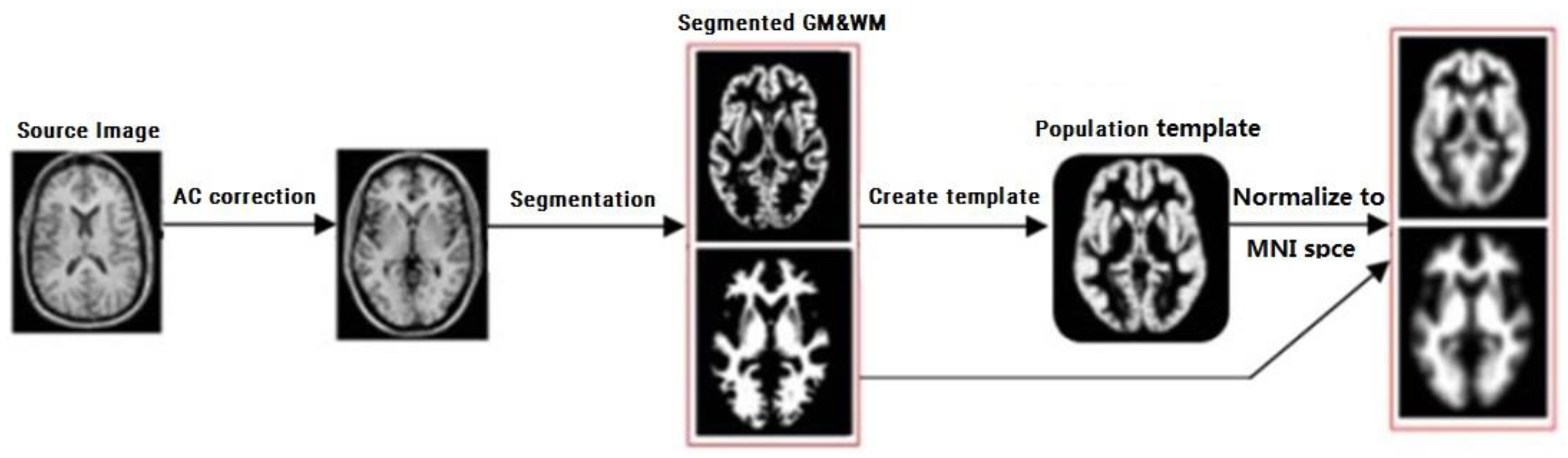
We first selected the Magnetisation Prepared Rapidly Acquired Gradient echo (MP-RAGE) to segment the MR images into gray matter (GM), white matter (WM), and Cerebrospinal Fluid (CSF). Then, the Diffeomorphic Anatomical Registration through Exponentiated Lie Algebra (DARTEL) algorithm was utilized for spatial normalization [26]. After spatial normalization, we applied the SPM8 package to structural brain image segmentation, and utilize the DARTEL algorithm to create an average-shaped template and normalize the segmented image to Montreal Neurological Institute (MNI) Space, respectively. The features are the GM probability maps in the MNI space. The procedure of DARTEL is shown as Figure 1.
2.2. Feature Extraction
After image processing, we utilized the Automatic Anatomical Labeling (AAL) binary atlas for the 3D case in the anatomical registration [27]. An anatomical parcellation of the spatially normalized single-subject high-resolution T1 volume provided by the Montreal Neurological Institute (MNI) was performed [28]. The MNI single-subject main sulci was first delineated and further used as landmarks for the 3D definition of 45 anatomical volumes of interest (AVOI) in each hemisphere. Then, the 90 AVOI was reconstructed and then assigned a label. Based on the previous results, we computed the GM tissue volume of the anatomical region and then produced 90 regions features for classification analysis.
2.3. Feature Selection
We have obtained 90 features that are based on the previous feature extraction. However, not all of the features can be used for Alzheimer’s Disease clinical diagnosis. Because some features may not be discriminative, these features are not helpful in diagnosis, and they may even affect diagnostic accuracy. To deal with this situation, we proposed a feature selection method that is based on the information gain in this section.
The concepts of information gain were discussed in the article: The Mathematical Theory of Communication by C.E. Shannon, 1949.
On the assumption that pij is the anatomical volume of gray matter of a single subject (j = 1, 2, 3, …, 90); m is the class number. The entropy of an attribute is:
If the number of the subjects per class is equal for both classes, H = 1. In the case of unbalanced class sizes the entropy of the class distribution is smaller than one and approaches zero if there are much more instances of one class than of the other class.
Based on the definition of entropy, we can define the information gain of a voxel, as follows:
where
where A is the attribute value of the feature examples, and B is the corresponding class label. The information gain scales are between 0 and 1. If IG(B) = 0, it indicates that the corresponding voxel provides no information on the class label of the subjects. On the other hand, if IG(B) = 1, it indicates that the class labels of all subjects can be derived from the corresponding voxel without any errors.
In relation to information gain, C4.5 statistical classifier, as developed by Ross Quinlan [29], has been implemented in this study. The decision tree was built from large sets of cases belonging to known classes. The cases, as described by mixture of nominal and numeric properties, are scrutinized for patterns that allow for the classes to be reliably discriminated. These patterns are then expressed as models, in the form of decision tree or sets of rules. At each node of the tree, C4.5 chooses the attribute of the data that most effectively splits its set of samples into subsets that are enriched in one class or the other. The splitting criterion is the normalized information gain. The attribute with the highest normalized information gain is chosen to make the decision. This is the process of feature selection, which is to learn from the training data that map from the attribute values to a predicted class.
3. Methods
We have obtained the optimal discriminant features for MRI images based on the previous feature extraction and selection steps. Then, we can utilize these features into Alzheimer’s Disease clinical diagnosis with the traditional diagnosis methods (i.e., k-nearest neighbor [30], support vector machine [31]). However, these traditional methods are all based on the assumption: the training and testing data are drawn from the same distribution. This identical-distribution assumption may not hold in the diagnosis of AD and MCI. Because the MRI image data of AD patient at different stages have a significant difference. If we use the traditional diagnosis methods in this situation, it may lead to a greater diagnostic error. Since the MRI image data of the AD patient at different stages can be viewed as data from different distributions. If we directly use the model that is trained in the dataset from one distribution to the dataset from another distribution, the accuracy of the diagnosis cannot be guaranteed. To solve this problem, the transfer learning method is utilized into the diagnosis of AD with the selected features in this section.
3.1. Problem Definition
Before we introduce the transfer learning method, we first use different symbols to represent patients at different stages. In particular, we let AD indicates patients with diagnosed Alzheimer’s Disease, MCI indicate patients with mild cognitive impairment. MCI may develop into AD, but it can also improve and recover. Hence, we consider AD and MCI as two different data set. The AD is considered as training data, MCI as testing data. The classification model based on AD as training data was then transferred to the MCI data for classification. Furthermore, the first group of MRI samples from the ADNI database was western population; the second group of MRI samples obtained from the local hospital was eastern population. The different features between these two groups of samples were also analyzed with the transfer learning method. The transfer learning model was established based on ADNI samples (training data) and it was implied to local samples (testing data) for diagnostic analysis.
Here, we define some of the necessary symbols using in the transfer learning method. Supposing that Td represents the diff-distribution training data (source domain), Ts represents the same-distribution training data (target domain). Both Td and Ts are labeled datasets, T = Td∪Ts. S is to indicate the test dataset. Our goal is to learn a model based on the labeled dataset T for the diagnostic tasks from S.
3.2. Transfer Learning Method for Alzheimer’s Disease Clinical Diagnosis
To solve the problem that happened in Alzheimer’s Disease clinical diagnosis that is caused by the training and testing data drawn from different distributions, we try to propose a transfer learning method for diagnosis by utilizing important weights. In our method, we first assign a weight for each image from training dataset. Then we try to adjust the weights to filter the images with the large difference from the testing data distribution. In this way, we can train a suitable model on the re-weighted data for the diagnostic tasks from testing data.
Specifically, we let wi indicates the importance weights for the i-th image. Then, we can use a weight vector W = (w1, w2, …, wn+m) to indicate the weights for training data. When considering the fact that the training dataset may include few labeled data from target domain, we use weights w1, …, wn to indicates weights for the source domain, and use weights wn+1, …, wn+m for the target domain.
To introduce the used transfer learning method, we present the TrAdaboost method in detail. In TrAdaboost, to obtain a suitable images weights, we initialize weight vector W by , and
In the first step, weight vector W1 is used to re-sample the images from training dataset. In the second step, we utilize traditional method to learn a base model, h1 with re-sampled dataset. After we obtain a base model, in the third step, we calculate the error e1 of h1 on S,
where, c(xi) indicates real label of image xi. To filter images with a large difference from testing data distribution, in the fourth step, the weight vector is updated, as following,
where β1 = e1/(1 − e1). Then new weight vector is used to repeat step 1 to step 4 until change of e is less than threshold ε.
For a test image x, the output hypothesis is:
where N indicates the maximum number of iterations.
4. Experiments
4.1. Data Setting
In this study, we analyzed the total 507 subjects of AD, MCI, and NC from ADNI database using Statistical Parametric Mapping (SPM), DARTEL procedure, and AAL template. The MR images from ADNI including 177 AD patients, 245 MCI patients, and 85 normal controls (NC) were served as experimental samples. All of the images were preprocessed with DARTEL toolbox and then mapped to the standard MNI space neurological coordinate system and Automated Anatomical Labeling (AAL). 90 AVOI were extracted as feature and then graphically depicted with Box-plot. Meanwhile, the mean of 90 AVOI for AD, MCI, and NC groups were calculated and compared with the line chart. Then, the information gains of 90 AVOI were calculated for feature selection.
Transfer learning algorithm was introduced into the classification analysis of AD, MCI, and NC. AD was used as training data and MCI as testing data in transfer learning. The testing result indicated that rather high accuracy and sensitivity had been achieved. Furthermore, the 90 AVOI were used to obtain information gains for feature selection. The impact of feature selection on classification accuracy was calculated. Finally, local AD subjects were analyzed with transfer learning module based on ADNI training data.
4.2. Evaluation Measure
The accuracy of each algorithm was utilized to evaluate the performance of the algorithms in the experimental results. For further detailed analysis of the results, another evaluation measure was used. For example, the fluctuation rate was illustrated with two Formulas (8) and (9), as follows:
ACCmax represents the maximum accuracy of each Src group, while ACCmin represents the minimum; ACC group set as the accuracy of AD/NC1 as Src in our algorithm.
The change rate of accuracy among all tested classification algorithm was also calculated with the various Tartrain sample sizes. The calculation formula is (10), as follows:
ACCmax is the maximum accuracy of each classification algorithm, and ACCmin is the minimum accuracy. Besides, the sensitivity and specificity were also calculated in this study.
4.3. Feature Selection Results
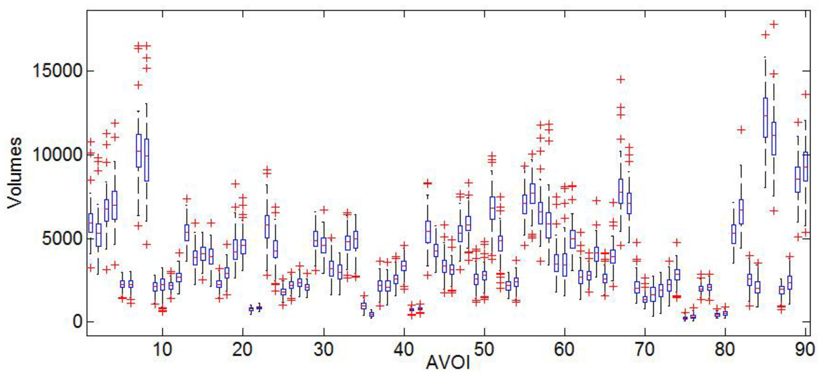
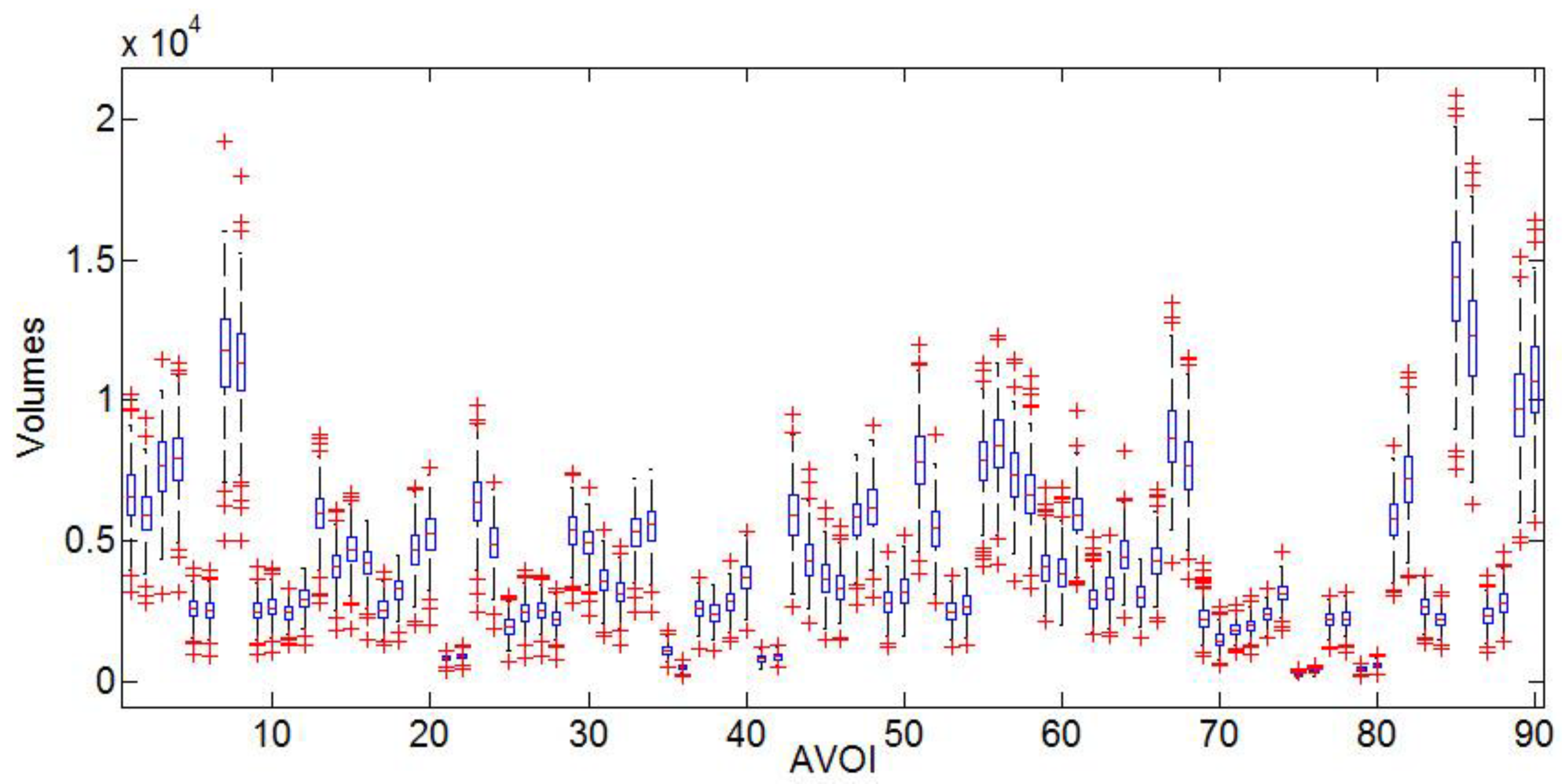
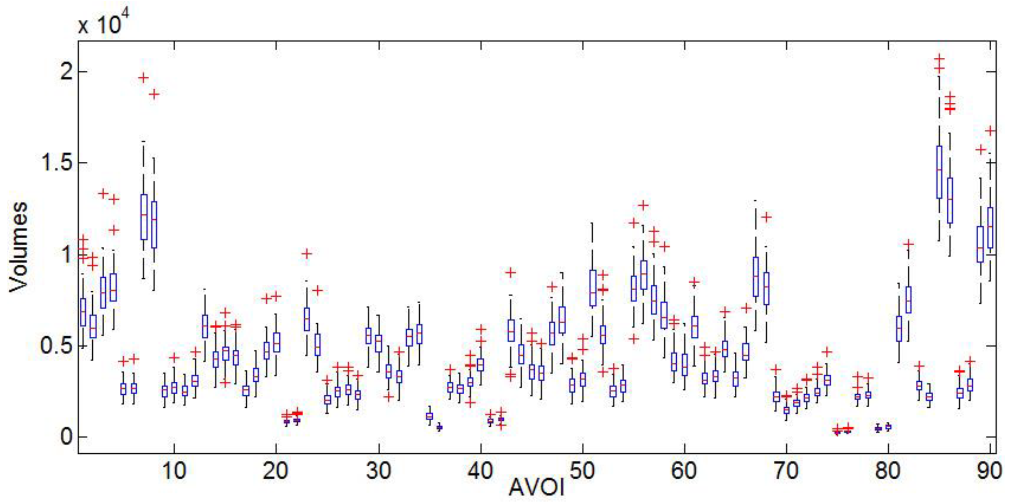
Box-plots display variation in 90 AVOI of AD, MCI, and NC groups, respectively. In the group of AD, the grey matter box-plots were illustrated as Figure 2, MCI showed in Figure 3 and NC showed in Figure 4. Referring to the figures, it can be seen that the group of NC has the lowest degree of dispersion, whereas the group of MCI has the highest one. The high degree of dispersion in MCI confirms the statistically significant difference in the volumes of gray matter, which is also consistent with the clinical characteristic of MCI. That is, part of MCI may turn to AD, while another part may keep stable or even turn to NC.
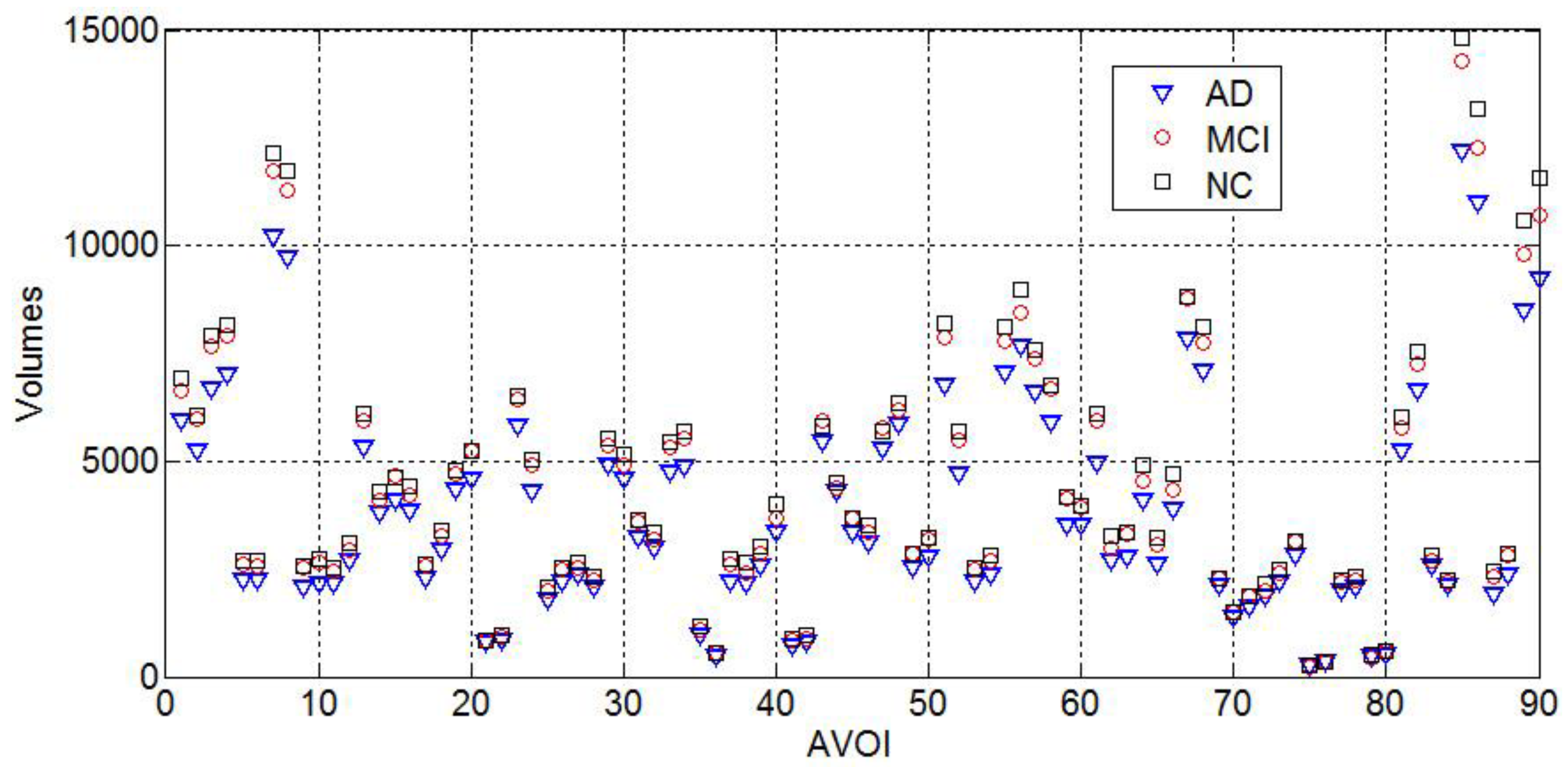
The mean grey matter volumes of 90 AVOI in AD, MCI, and NC classed are shown in Figure 5. Figure 5 shows that the AD group has the smallest mean gray matter volume for every AVOI, whereas NC group has the largest one. This is also consistent with clinical evidence of significant atrophy of gray matter in AD patients and the mild atrophy in MCI patients.
Based on the feature, the grey matter volume of 90 AVOI data was divided into two groups and analyzed with information entropy. The first group is AD vs. NC, including 177 AD and 85 NC subjects; the other group is MCI vs. NC, including 245 MCI and 85 NC subjects. The information gains of 90 AVOI data was calculated with Formulas (1)–(3). The values were sorted and the top 15 The information gains of anatomical regions are shown in Table 3.
Based on information gain, we selected just seven anatomical regions as feature and got good classification performance. These seven common regions were highlighted in bold and then identified in the top 15 anatomical regions, which had higher information gain among both AD and MCI groups. These selected seven regions were consistent with the grey matter volume atrophy in AD and MCI subjects that had been reported in various literatures [32]. For example, both AD and MCI patients appeared to have various degrees of atrophy in hippocampus and amygdala regions. Results in Figure 2 showed that the atrophy of common regions had tight relation with AD and MCI, such as Hippocampus (No. 37–No. 38), Parahippocampal gyrus (No. 40), and Amygdala (No. 41–No. 42). The atrophy in these seven regions was more severe in AD patients than MCI patients. So, we selected these seven anatomical regions as feature, which were applied into the transfer learning algorithm from AD to MCI subjects.
Based on the evidences of the anatomical regions with the highest 15 information gains being shown on Table 3, a total of seven regions, including left and right hippocampus, left and right amygdala, right parahippocampal gyrus, left angular gyrus, and Inferior temporal gyrus, were presented in both compared groups. These regions have also been reported in other studies, suggesting brain volume loss in these regions in both the AD and MCI group [33]. For example, both AD and MCI patients appeared to have various degrees of volume loss in left and right hippocampus, left and right amygdala, and right parahippocampal gyrus. In subsequent experiments, we also discussed the accuracy of classification using the AVOI of seven common regions as feature.
4.4. Transfer Learning Results
We defined “Src” as training data in source domain, “Tartrain” as training data in target domain, and “Tartest” as testing data in target domain. In this study, transfer learning includes three parts. In the first part, the accuracy of the classification with AD was explored as training data and MCI as testing data. In the second part, the common anatomical regions in both information gain ranged groups, AD vs. NC and MCI vs. NC, was selected as feature. These features were then examined using feature iterative optimization for their impact on accuracy. In the final part, the ADNI subjects were set as the training data and the testing data was from the local hospital. Obviously, there were big differences in ethnicity and sample size between these two data sets. In this context, we explored whether or not transfer learning was still valid for transferring the knowledge that was learned from ADNI data to local hospital data.
4.5. Results on Transfer Task: AD → MCI
177 AD and 40 NC subjects were grouped as training data; 245 MCI and 45 remaining NC subjects were combined as testing data. Since some studies indicated the possibility of inadequate classification due to imbalance sample sizes, we divided AD data into four groups, MCI data into two groups, and NC data into three groups, details of each group were shown in Table 4 (the last group in AD was AD which contained all 177 AD subjects). In this way, we set AD1 and NC1, AD2 and NC1, AD3 and NC1, and AD4 and NC1 as Src, respectively; MCI1 and NC3 as Tartrain; and, MCI2 and NC2 as Tartest. Then, the sample sizes of MCI1 and NC3 would be increased in the following experiments, as we exam the assumption of consistency between the size of Tartrain and the accuracy of classification. The proposed transfer learning method was compared with four classic classification algorithms, i.e., SVM, KNN, ITML, and Linear-MSVM. For the sake of fairness, the same Src, Tartrain, and Tartest were used in all methods. The classification performances based on all five methods are listed in Table 5.
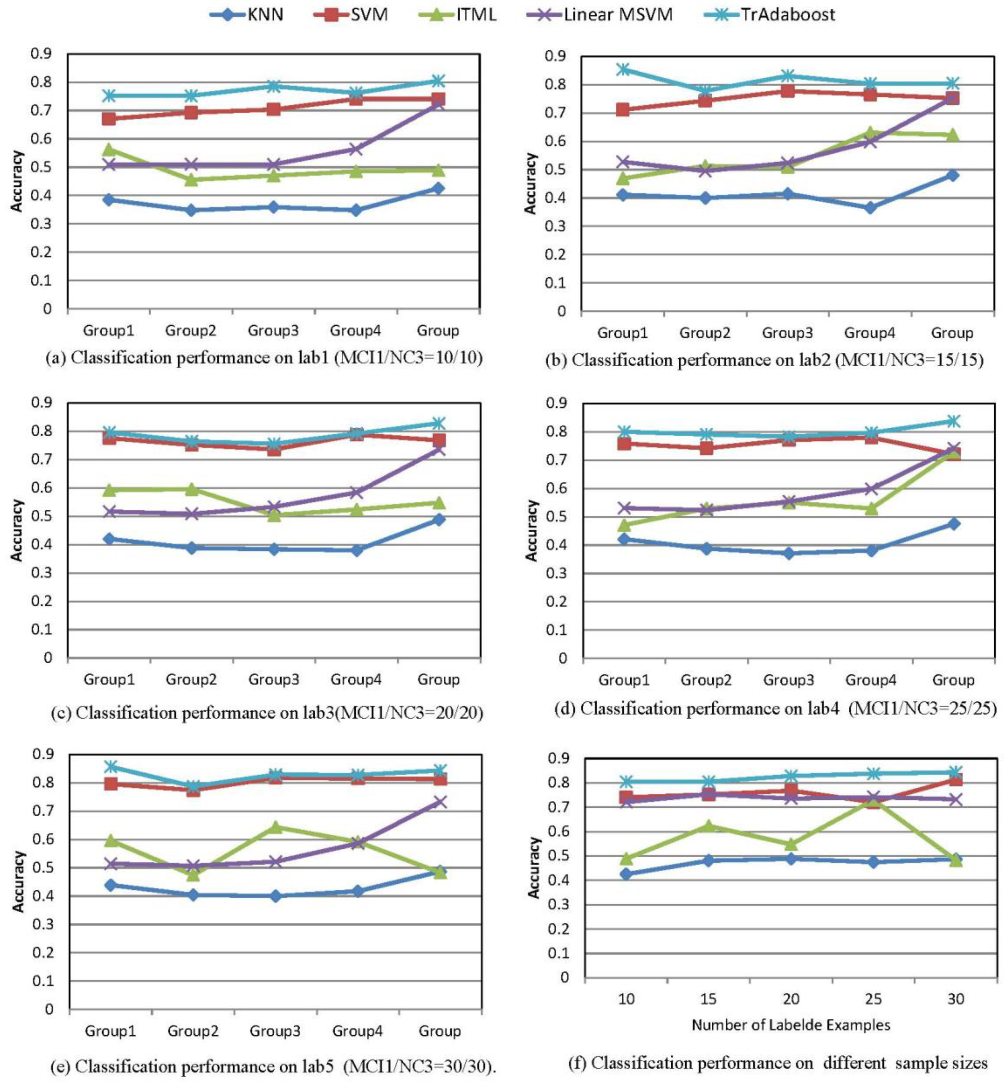
As shown in Figure 6a, the accuracy of tour algorithm is 80.44%, which is significantly higher than the other four algorithms. Furthermore, we studied the impact on classification accuracy according to the change of Tartrain size. Parallel with the division method in Table 4, we ran the test with MCI1/NC3 (Tartrain) size at 15, 20, 25, and 30, respectively (see Lab2–Lab5). The accuracy of classification on five methods was listed in Figure 6b–e for the different Tartrain size. Figure 6a–e showed that the accuracy of proposed algorithm achieved the highest scores among all five methods. Meanwhile, we could see there was no significant difference in the TrAdaboost algorithm among all Src groups, which suggests that Src grouping has little impact on the accuracy of TrAdaboost algorithm. In comparison, the AD/NC1 group as Src appeared to have higher accuracy in the other four classic methods, but it obviously lacked stability. Based on the above results, we concluded that dividing the training data has no significant influence on the accuracy of transfer learning method. It also suggests that the results are more reliable with a bigger sample size. Consequently, the training data was no longer divided in the following experiments, and we just used AD/NC1 as Src data.
When comparing Figure 6a with Figure 6e, the accuracy of our algorithm fluctuated the most in Figure 6b, and the details are listed in Table 6. Based on the various sizes of Tartrain data, the classification performance on AD/NC1 group were shown in Figure 6e and Table 7. The classification results showed that our algorithm had the highest accuracy among all five methods. Moreover, in Figure 6e, we can see the classification accuracy in TrAdaboost algorithm increased as the sample size of Tartrain increased. The details are listed in Table 7.
4.6. Results on Transfer Task: ADNI → Local Hospital Data
In the final part of the study, we constructed the classification module based on ADNI samples, and then transferred the knowledge to the local hospital subjects. Meanwhile, the Accuracy (ACC), Sensitivity (SEN), and Specificity (SPE) were calculated in order to assess the validation of this module in clinical diagnosis. ACC, SEN, and SPE results were shown in Table 8. As the result showed, the transfer learning module achieved high accuracy, sensitivity, and specificity. We conclude that this method is efficient and valuable in assisting clinical diagnosis.
In the classification of local AD subjects using the “knowledge” learned from ADNI data and TrAdaboost algorithm (Table 8), classification accuracy had all gone beyond 90% on each Tartrain group. The top accuracy was recorded at 93.75% with Tartrain AD1/NC1 set at 2/2, while sensitivity was 80%, and specificity was 1. Obviously, the proposed transfer learning module was effective. According to Tabel 9, the Youden indexes could be calculated on each Tartrain group. The Youden indexes were 0.875, 0.857, 0.833, 0.8, 0.875, and 0.833 respectively, apparently all gone beyond 0.7. Therefore, we could conclude that TrAdaboost algorithm is valuable in assisting clinical diagnosis.
4.7. The Efficiency of TrAdaboost Algorithm
In this study, we tested and verified that the transfer learning algorithm had higher accuracy and stability than some classic algorithms.
To keep the balance of sample sizes for better classification performance, we divided the AD, MCI, and NC data into small groups, as shown in Table 4. Then, the classification accuracy was calculated based on AD as training data and MCI as testing data with different grouping combinations. To have a better understanding of the efficiency of the TrAdaboost algorithm, we also applied classic algorithms, including SVM (support vector machine), KNN (K-nearest neighbor), ITML (information theory metric learning), and Linear-MSVM (linear metric based support vector machine). The accuracy of each algorithm was compared and studied with MCI1/NC3 as training data in target domain (Tartrain) whose sample size set at 10/10; AD1/NC1, AD2/NC1, AD3/NC1, AD4/NC1, and AD/NC1 as training data in source domain (Src), respectively. As shown in Table 5 and Figure 6a, TrAdaboost algorithm clearly outperformed other compared algorithms, with 80.44% as compared with 42.5% in KNN, 74.07% in SVM, 56.3% in ITML, and 72.1% in Linear-MSVM.
The findings in Figure 6b–e indicated that accuracy of TrAdaboost algorithm fluctuated mostly when the TarTrain MCI1/NC1 was 15/15 and AD1/NC1, AD2/NC1, AD3/NC1, AD4/NC1, and AD/NC1 were the source domain training data (Src).
With the Formulas (8), (9) and data shown in Table 6, the ratetop and ratebott was calculated as 5.77% and 3.25% respectively. It shows that using AD/NC1 as Src has no significant difference with other Src groups, i.e., AD1/NC1, AD2/NC1, AD3/NC1, and AD4/NC1. Since the test result would be more stable with larger sample size, we no longer considered other Src groups, just used AD/NC1 as Src in the experiments of selected feature and local hospital subjects.
This study also examined the classification accuracy of different algorithms with different Tartrain sample size. The results in Figure 6a–e and Table 7 showed that when Tartrain MCI1/NC3 was 15/15 with Src was AD/NC1, the classification accuracy of SVM, KNN, ITML, Linear-MSVM, and TrAdaboost algorithm were 0.7523, 0.4808, 0.623077, 0.753036, and 0.804615, respectively. TrAdaboost algorithm achieved the highest accuracy in all tested methods. Similarly, our algorithm had the highest accuracy among all the tested methods, as the sample size of MCI1/NC3 was altered to 20/20, 25/25, and 30/30 (Table 7).
The data in Table 7 and Formula (10) were used to calculate the change rate of accuracy. The results indicated that the change rate of SVM, KNN, ITML, and Linear-MSVM and our algorithm was 12.79%, 14.69%, 51.09%, 4.37%, and 4.85%, respectively. It was clear that Linear-MSVM and our algorithm had lower fluctuation of accuracy and more stable comparing with the other three algorithms. Combined with accuracy and stability, our algorithms had outperformed other tested methods.
5. Conclusions
This research introduced transfer learning module into the classification of AD, MCI, and NC. The results show that TrAdaboost algorithm has a clear advantage over classic classification methods with higher accuracy and less fluctuation. Moreover, with transfer “knowledge” from the ADNI database to a local database, TrAdaboost algorithm achieves high accuracy, sensitivity, and specificity, which indicates its value in clinical application. In addition, we applied information gain method to optimize the feature selection in transfer learning. The results show that the classification accuracy is improved with the optimized feature selection, which indicates that information gain method can be used to select the more sensitive anatomical regions in AD and MCI diagnosis. In future work, better feature optimization will be explored in the transfer learning module in order to improve its accuracy and consistency. Except better feature optimization, the challenge when diverse databases are involved will be taken into consideration for the future work. For example, how to filter redundant information in different databases or how to migrate knowledge-assisted diagnostics between heterogeneous data. These are all questions that are worth studying. Furthermore, our research just distinguishes AD from normal individuals, but many other conditions manifests dementia in clinical, such as Lewy body disease, vascular dementia, etc. How to use artificial intelligent assisting radiological diagnosis to discriminate AD from other types of dementia will be taken into consideration for the future work.
Author Contributions
K.Z. Conceptualization, Formal analysis, Funding acquisition, Methodology, Project administration, Resources, Validation, Writing-original draft; W.H., Validation, Writing-review & editing; Y.X., Conceptualization, Methodology, Supervision, Writing-review & editing, Funding acquisition; G.X., Supervision, Validation; J.C., Methodology, Formal analysis, Writing-original draft, Writing-review & editing.
Funding
This research was funded by Medical Scientific research foundation of Guangdong Province, China (NO. A2017278); Science and Technology Project of Zhanjiang, China (No. 2015A01039). Especially, Yonghui Xu thanks the support of Project funded by China Postdoctoral Science Foundation (No. 2018M630945) and the International Postdoctoral Exchange Fellowship Program.
Conflicts of Interest
The authors declare no conflicts of interest.
References
- Jellinger, K.A. Mild cognitive impairment. Aging to alzheimer’s disease. Eur. J. Neurol. 2003, 10, 466. [Google Scholar] [CrossRef]
- Ritter, K.; Schumacher, J.; Weygandt, M.; Buchert, R.; Allefeld, C.; Haynes, J.D. Multimodal prediction of conversion to alzheimer’s disease based on incomplete biomarkers. Alzheimers Dement. 2015, 1, 206–215. [Google Scholar]
- Karas, G.B.; Burton, E.J.; Rombouts, S.A.R.B.; van Schijndel, R.A.; Brien, J.T.O.; Scheltens, P.H.; McKeith, I.G.; Williams, D.; Ballard, C.; Barkhof, F. A comprehensive study of gray matter loss in patients with alzheimer’s disease usingoptimized voxel-based morphometry. NeuroImage 2003, 18, 895–907. [Google Scholar] [CrossRef]
- Hinrichs, C.; Singh, V.; Xu, G.; Johnson, S.C. Predictive markers for ad in a multi-modality framework: An analysis of mci progression in the adni population. NeuroImage 2011, 55, 574–589. [Google Scholar] [CrossRef] [PubMed]
- Young, J.; Modat, M.; Cardoso, M.J.; Mendelson, A.; Cash, D.; Ourselin, S. Accurate multimodal probabilistic prediction of conversion to alzheimer’s disease in patients with mild cognitive impairment. NeuroImage Clin. 2013, 2, 735–745. [Google Scholar] [CrossRef] [PubMed]
- Leon, M.J.D.; Mosconi, L.; Li, J.; Santi, S.D.; Yao, Y.; Tsui, W.H.; Pirraglia, E.; Rich, K.; Javier, E.; Brys, M. Longitudinal csf isoprostane and mri atrophy in the progression to ad. J. Neurol. 2007, 254, 1666–1675. [Google Scholar] [CrossRef] [PubMed]
- Fjell, A.M.; Walhovd, K.B.; Fennema-Notestine, C.; McEvoy, L.K.; Hagler, D.J.; Holland, D.; Brewer, J.B.; Dale, A.M.; Alzheimer’s Disease Neuroimaging Initiative. Csf biomarkers in prediction of cerebral and clinical change in mild cognitive impairment and alzheimer’s disease. J. Neurosci. Off. J. Soc. Neurosci. 2010, 30, 2088–2101. [Google Scholar] [CrossRef] [PubMed]
- Du, A.T.; Schuff, N.; Kramer, J.H.; Rosen, H.J.; Gornotempini, M.L.; Rankin, K.; Miller, B.L.; Weiner, M.W. Different regional patterns of cortical thinning in alzheimer’s disease and frontotemporal dementia. Brain 2007, 130, 1159–1166. [Google Scholar] [CrossRef] [PubMed]
- Friston, K.J.; Poline, J.B.; Holmes, A.P.; Frith, C.D.; Frackowiak, R.S. A multivariate analysis of pet activation studies. Hum. Brain Mapp. 2015, 4, 140–151. [Google Scholar] [CrossRef]
- Mckeown, M.J.; Makeig, S.; Brown, G.G.; Jung, T.P.; Kindermann, S.S.; Bell, A.J.; Sejnowski, T.J. Analysis of fMRI data by blind separation into independent spatial components. Hum. Brain Mapp. 1998, 6, 160–188. [Google Scholar] [CrossRef] [Green Version]
- Mourao-Miranda, J.; Bokde, A.L.; Born, C.; Hampel, H.; Stetter, M. Classifying brain states and determining the discriminating activation patterns: Support vector machine on functional MRI data. Neuroimage 2005, 28, 980–995. [Google Scholar] [CrossRef] [PubMed]
- Mourao-Miranda, J.; Reynaud, E.; Mcglone, F.; Calvert, G.; Brammer, M. The impact of temporal compression and space selection on SVM analysis of single-subject and multi-subject fMRI data. Neuroimage 2007, 33, 1055–1065. [Google Scholar] [CrossRef] [PubMed]
- Xu, Y.; Pan, S.J.; Xiong, H.; Wu, Q.; Luo, R.; Min, H.; Song, H. A unified framework for metric transfer learning. IEEE Trans. Knowl. Data Eng. 2017, 29, 1158–1171. [Google Scholar] [CrossRef]
- Xu, Y.; Min, H.; Song, H.; Wu, Q. Multi-instance multi-label distance metric learning for genome-wide protein function prediction. Comput. Biol. Chem. 2016, 63, 30–40. [Google Scholar] [CrossRef] [PubMed]
- Xu, Y.; Min, H.; Wu, Q.; Song, H.; Ye, B. Multi-instance metric transfer learning for genome-wide protein function prediction. Sci. Rep. 2017, 7, 41831. [Google Scholar] [CrossRef] [PubMed]
- Schmidhuber, J. On Learning How to Learn learning strategies (Technical Report FKI-198-94); Fakultat fur Informatik: Munich, Germany, 1995. [Google Scholar]
- Thrun, S.; Mitchell, T.M. Learning one more thing. In Proceedings of the International Joint Conference on Artificial Intelligence, Montreal, QC, Canada, 20–25 August 1995; pp. 1217–1223. [Google Scholar]
- Caruana, R. Multitask learning. Mach. Learn. 1997, 28, 41–75. [Google Scholar] [CrossRef]
- Ben-David, S.; Schuller, R. Exploiting task relatedness for multiple task learning. In Proceedings of the Computational Learning Theory and Kernel Machines, Conference on Computational Learning Theory and Kernel Workshop, Colt/Kernel 2003, Washington, DC, USA, 24–27 August 2003; pp. 567–580. [Google Scholar]
- Daumé, I.H.; Marcu, D. Domain adaptation for statistical classifiers. J. Artif. Intell. Res. 2011, 26, 101–126. [Google Scholar] [CrossRef]
- Hoffman, J.; Rodner, E.; Donahue, J.; Darrell, T.; Saenko, K. Efficient learning of domain-invariant image representations. arXiv, 2013; arXiv:1301.3224. [Google Scholar]
- Liu, Y.; Stone, P. Value-function-based transfer for reinforcement learning using structure mapping. In Proceedings of the National Conference on Artificial Intelligence and the Eighteenth Innovative Applications of Artificial Intelligence Conference, Boston, MA, USA, 16–20 July 2006. [Google Scholar]
- Soni, V.; Singh, S. Using homomorphisms to transfer options across continuous reinforcement learning domains. In Proceedings of the National Conference on Artificial Intelligence, Boston, MA, USA, 16–20 July 2006; pp. 494–499. [Google Scholar]
- Schéulkopf, B.; Platt, J.; Hofmann, T. Dirichlet-enhanced spam filtering based on biased samples. In Proceedings of the 19th International Conference on Neural Information Processing Systems, Vancouver, BC, Canada, 4–7 December 2006; pp. 161–168. [Google Scholar]
- Mueller, S.G.; Weiner, M.W.; Thal, L.J.; Petersen, R.C.; Jack, C.; Jagust, W.; Trojanowski, J.Q.; Toga, A.W.; Beckett, L. The Alzheimer’s disease neuroimaging initiative. Neuroimaging Clin. N. Am. 2005, 15, 869. [Google Scholar] [CrossRef] [PubMed]
- Ashburner, J. A fast diffeomorphic image registration algorithm. NeuroImage 2007, 38, 95–113. [Google Scholar] [CrossRef] [PubMed]
- Tzourio-Mazoyer, N.; Landeau, B.; Papathanassiou, D.; Crivello, F.; Etard, O.; Delcroix, N.; Mazoyer, B.; Joliot, M. Automated anatomical labeling of activations in spm using a macroscopic anatomical parcellation of the mni mri single-subject brain. NeuroImage 2002, 15, 273–289. [Google Scholar] [CrossRef] [PubMed]
- Stjean, P.; Sadikot, A.F.; Collins, L.; Clonda, D.; Kasrai, R.; Evans, A.C.; Peters, T.M. Automated atlas integration and interactive three-dimensional visualization tools for planning and guidance in functional neurosurgery. IEEE Trans. Med. Imaging 1998, 17, 672–680. [Google Scholar] [CrossRef] [PubMed]
- Salzberg, S.L. Book Review: C4.5: Programs for Machine Learning by J. Ross Quinlan; Morgan Kaufmann Publishers, Inc.: Burlington, MA, USA, 1993; Kluwer Academic Publishers: Dordrecht, The Netherlands, 1994. [Google Scholar]
- Aha, D.W.; Kibler, D.; Albert, M.K. Instance-Based Learning Algorithms; Kluwer Academic Publishers: Dordrecht, The Netherlands, 1991. [Google Scholar]
- Vapnik, V.N. Statistical Learning Theory. Adaptive and Learning Systems for Signal Processing; Communications and Control Series; John Wiley & Sons: Hoboken, NJ, USA, 1998. [Google Scholar]
- Xin, B.; Kawahara, Y.; Wang, Y.; Hu, L.; Gao, W. Efficient generalized fused lasso and its applications. ACM Trans. Intell. Syst. Technol. 2016, 7, 1–22. [Google Scholar] [CrossRef]
- Chételat, G.; Landeau, B.; Eustache, F.; Mézenge, F.; Viader, F.; De, L.S.V.; Desgranges, B.; Baron, J.C. Using voxel-based morphometry to map the structural changes associated with rapid conversion in mci: A longitudinal mri study. Neuroimage 2005, 27, 934–946. [Google Scholar] [CrossRef] [PubMed]
Figure 1.
The procedure of the Diffeomorphic Anatomical Registration through Exponential Lie Algebra.
Figure 1.
The procedure of the Diffeomorphic Anatomical Registration through Exponential Lie Algebra.

Figure 2.
Alzheimer’s Disease (AD) grey matter volume Box-plot.

Figure 3.
Mild cognitive impairment (MCI) grey matter volume Box-plot.

Figure 4.
Normal controls (NC) grey matter volume Box-plot.

Figure 5.
Mean of grey matter volumes of 90 anatomical volumes of interest (AVOI).

Figure 6.
Comparison results.


Table 1.
ADNI Subject Information.
| Group | AD | MCI | NC |
|---|---|---|---|
| Sample size (male/female) | 93/84 | 155/90 | 42/43 |
| Age (years ± SD) | 75.6 ± 7.7 | 75 ± 7.7 | 75.9 ± 5.5 |
| CDR (0/0.5/1/2) | 0/81/94/2 | 0/245/0/0 | 85/0/0/0 |
| MMSE | 23.07 ± 2.4 | 26.58 ± 2 | 29.06 ± 0.9 |
Table 2.
Local Subject Information.
| Group | AD (n = 18) | NC (n = 18) |
|---|---|---|
| Sample size (male/female) | 8/10 | 8/10 |
| Age (years ± SD) | 64.6 ± 1.8 | 67.9 ± 1.8 |
| CDR (0/0.5/1/2) | 0/0/12/6 | 18/0/0/0 |
| MMSE | 10.7 ± 1.2 | 28.86 ± 0.2 |
Table 3.
The top 15 Information gains of anatomical region.
| AD vs. NC | MCI vs. NC | ||
|---|---|---|---|
| Amygdala_L, Amygdala | 0.259 | Hippocampus_R, Hippocampus | 0.045 |
| Inferior temporal gyrus | 0.237 | Heschl_L, Heschl gyrus | 0.042 |
| Temporal_Inf_L, Inferior temporal gyrus | 0.220 | Caudate_R, Caudate nucleus | 0.039 |
| Amygdala_R, Amygdala | 0.217 | Frontal_Inf_Oper_R, Inferior frontal gyrus | 0.038 |
| Temporal_Pole_Mid_L, middle temporal gyrus | 0.215 | SupraMarginal_R, Supramarginal gyrus | 0.034 |
| Frontal_Mid_Orb_L, Middle frontal gyrus | 0.214 | Amygdala_L, Amygdala | 0.033 |
| Temporal_Mid_L, Middle temporal gyrus | 0.213 | Temporal_Inf_R, Inferior temporal gyrus | 0.031 |
| Frontal_Mid_L, Middle frontal gyrus | 0.208 | Angular_L, Angular gyrus | 0.030 |
| Frontal_Inf_Oper_L, Inferior frontal gyrus | 0.180 | Angular_R, Angular gyrus | 0.030 |
| Hippocampus_L, Hippocampus | 0.180 | ParaHippocampal_R, Parahippocampal gyrus | 0.029 |
| Hippocampus_R, Hippocampus | 0.176 | Amygdala_R, Amygdala | 0.029 |
| Frontal_Sup_Orb_L, Superior frontal gyrus | 0.172 | Supramarginal gyrus | 0.029 |
| ParaHippocampal_R, Parahippocampal gyrus | 0.171 | Hippocampus_L, Hippocampus | 0.029 |
| Angular_L, Angular gyrus | 0.171 | Temporal_Mid_R, Middle temporal gyrus | 0.027 |
Table 4.
Detailed information of data setting.
| Data Set | |||||
|---|---|---|---|---|---|
| AD (177) | Group | Sample size | Group | Sample size | |
| AD1 | 40 | MCI (245) | MCI1 | 10 | |
| AD2 | 40 | MCI2 | 235 | ||
| AD3 | 40 | NC (85) | NC1 | 40 | |
| AD4 | 57 | NC2 | 35 | ||
| NC3 | 10 | ||||
Table 5.
Classification performance of five methods on different Src groups.
| Groups | KNN | SVM | ITML | Linear MSVM | TrAdaboost |
|---|---|---|---|---|---|
| Group 1 | 0.385 | 0.671 | 0.563 | 0.510 | 0.752 |
| Group 2 | 0.348 | 0.692 | 0.455 | 0.510 | 0.752 |
| Group 3 | 0.359 | 0.7037 | 0.470 | 0.51 | 0.785 |
| Group 4 | 0.3481 | 0.7407 | 0.485 | 0.5641 | 0.762 |
| Group 5 | 0.425 | 0.741 | 0.488 | 0.721 | 0.804 |
Table 6.
Lab2 The accuracy of TrAdaboost algorithm on different Src groups.
| Group1 | Group2 | Group3 | Group4 | Group5 | |
|---|---|---|---|---|---|
| Accuracy | 0.854 | 0.778 | 0.831 | 0.804 | 0.804 |
Table 7.
Accuracy of test algorithms in different Tar-test sample sizes.
| 10 | 15 | 20 | 25 | 30 | |
|---|---|---|---|---|---|
| KNN | 0.425 | 0.481 | 0.488 | 0.475 | 0.487 |
| SVM | 0.7407 | 0.752 | 0.768 | 0.721 | 0.813 |
| ITML | 0.489 | 0.623 | 0.548 | 0.729 | 0.482 |
| Linear MSVM | 0.721 | 0.753 | 0.735 | 0.741 | 0.733 |
| TrAdaboost | 0.804 | 0.804 | 0.828 | 0.837 | 0.843 |
Table 8.
Accuracy (ACC), Sensitivity (SEN), and Specificity (SPE) results.
| Training Data | Testing Data | Results | |||
|---|---|---|---|---|---|
| AD/NC | AD1/NC1 | AD2/NC2 | Acc | Sen | Spc |
| AD (177) NC (85) | AD1/NC1(2/2) | AD2/NC2(16/16) | 0.9375 | 0.875 | 1 |
| AD1/NC1(4/4) | AD2/NC2(14/14) | 0.928571 | 0.8571 | 1 | |
| AD1/NC1(6/6) | AD2/NC2(12/12) | 0.916667 | 0.8333 | 1 | |
| AD1/NC1(8/8) | AD2/NC2(10/10) | 0.9 | 0.8 | 1 | |
| AD1/NC1(10/10) | AD2/NC2(8/8) | 0.9375 | 0.875 | 1 | |
| AD1/NC1(12/12) | AD2/NC2(6/6) | 0.916667 | 0.833333 | 1 | |
© 2018 by the authors. Licensee MDPI, Basel, Switzerland. This article is an open access article distributed under the terms and conditions of the Creative Commons Attribution (CC BY) license (http://creativecommons.org/licenses/by/4.0/).
Share and Cite
MDPI and ACS Style
Zhou, K.; He, W.; Xu, Y.; Xiong, G.; Cai, J. Feature Selection and Transfer Learning for Alzheimer’s Disease Clinical Diagnosis. Appl. Sci. 2018, 8, 1372. https://doi.org/10.3390/app8081372
AMA Style
Zhou K, He W, Xu Y, Xiong G, Cai J. Feature Selection and Transfer Learning for Alzheimer’s Disease Clinical Diagnosis. Applied Sciences. 2018; 8(8):1372. https://doi.org/10.3390/app8081372
Chicago/Turabian StyleZhou, Ke, Wenguang He, Yonghui Xu, Gangqiang Xiong, and Jie Cai. 2018. "Feature Selection and Transfer Learning for Alzheimer’s Disease Clinical Diagnosis" Applied Sciences 8, no. 8: 1372. https://doi.org/10.3390/app8081372
Note that from the first issue of 2016, this journal uses article numbers instead of page numbers. See further details here.