Electricity Generation in LCA of Electric Vehicles: A Review


1
Mat4En2—Materials for Energy and Environment, Dipartimento di Chimica, Materiali e Ingegneria Chimica “Giulio Natta”, Politecnico di Milano, Piazza Leonardo da Vinci 32, 20133 Milano, Italy
2
MOBI—Mobility, Logistics and Automotive Technology Research Centre, Department of Electric Engineering and Energy Technology, Vrije Universiteit Brussel, Pleinlaan 2, 1050 Brussels, Belgium
3
Flanders Make, 3001 Heverlee, Belgium
*
Author to whom correspondence should be addressed.
Appl. Sci. 2018, 8(8), 1384; https://doi.org/10.3390/app8081384
Submission received: 25 July 2018
/
Revised: 10 August 2018
/
Accepted: 13 August 2018
/
Published: 16 August 2018
(This article belongs to the Special Issue Plug-in Hybrid Electric Vehicle (PHEV))
Abstract
:Life Cycle assessments (LCAs) on electric mobility are providing a plethora of diverging results. 44 articles, published from 2008 to 2018 have been investigated in this review, in order to find the extent and the reason behind this deviation. The first hurdle can be found in the goal definition, followed by the modelling choice, as both are generally incomplete and inconsistent. These gaps influence the choices made in the Life Cycle Inventory (LCI) stage, particularly in regards to the selection of the electricity mix. A statistical regression is made with results available in the literature. It emerges that, despite the wide-ranging scopes and the numerous variables present in the assessments, the electricity mix’s carbon intensity can explain 70% of the variability of the results. This encourages a shared framework to drive practitioners in the execution of the assessment and policy makers in the interpretation of the results.
1. Introduction
Electric mobility is gaining momentum as a promising technology for decarbonisation of the transport sector and lots of scientific papers assessing environmental impacts of electric vehicles (EVs) are being produced. However, as the literature grows, so do the number of conflicting results.
A few reviews have tried to find a pattern in the Life Cycle Assessment (LCA) results: Hawkins et al. [1] identify the lack of a transparent and complete Life Cycle Inventory (LCI) as one of the main gaps in LCA. On the other hand, a more recent review by Nordelöf et al. [2] argues that the absence of a complete goal definition is the main hurdle to correctly interpret results and find trends in the literature.
Since the goal dictates the line for the subsequent scope and defines the applications of the study, omitting this phase leaves the study as a missive without address in the scientific community, and thus potentially ineffective.
Hawkins et al. [1] focused on the necessity to find consensus on the inventory. At the time of Hawkins’ publication, it was found that most studies limited their attention to a well-to-wheel analysis—since the use phase was seen to dominate the life cycle of vehicles, or to the battery production. The author’s purpose was then to investigate all those aspects that were not sufficiently addressed, providing the practitioner with a standardised system boundary and a set of relevant sub-components that could be distinguishable in the production phase.
The main causes of divergence in the literature, which make it difficult to compare studies are identified as follows by Hawkins et al. [1]: Different system boundaries, different level of detail and quality in the datasets, different lifetimes, different vehicles’ typologies and masses, battery technologies, vehicles performances, and then the electricity mix.
Nordelöf et al. [2] present an exhaustive analysis, and performs various meta-analyses from the findings of LCAs. They also widen the discussion to impact categories like resource depletion and toxicity, while the Hawkins’s focus remained on climate change.
Both reviews identified electricity production as the most impactful phase when it comes to climate change, and agreed on the need to find consensus on the appropriate electricity mix.
Since these two seminal reviews have been published, a variety of papers appeared in the literature, paving the way to new and interesting discussions as well as diverging results and methods.
A significant change in the way to account for electricity in the use phase of electric vehicles has occurred in the last few years: from an overgeneralisation of the inventory, using generic datasets (from EcoInvent, Emissions & Generation Resource Integrated Database [eGRID], Greenhouse gases Regulated Emissions and Energy use in Transportation [GREET], etc.…), the trend in the most recent LCAs has been a high detail of temporal and spatial variability, following the work by Graff Zivin et al. [3].
A blossoming of different methods to account for the “correct” electricity mix has led to lots of different, and sometime conflicting, results.
Lack of consensus in LCI data selection and lack of clear goal definitions are still the key factors to explain the difficult path of providing policy makers with robust and clear results.
This review analyses the methodological choices made by the scientific papers when assessing EVs. Since its relevance has been proved, a special focus is placed on electricity generation. The aim is to find a trend in accounting for the electricity production method, thus helping users navigate the conflicting results found in the literature, providing guidelines for future EVs studies and informing policy makers on the right method to use when assessing political choices.
2. Method
2.1. Articles Selection
The review analyses 44 LCA studies available in Scopus and Web of Science databases, published between 2008 and 2018, in which at least one of the analysed vehicles has an electric powertrain. This way both LCAs focusing only on electric vehicles (EVs) or hybrid electric vehicles (HEVs) and both comparative studies between traditional cars and electric vehicles are included.
The review includes both complete LCAs and Well-to-Wheel analysis, following the classification accepted in the literature [2]. A well-to-wheel (WtW) analysis is a partial LCA, which limits its system boundary to the cycle of the energy carrier used to propel the vehicle, such as liquid fuel or electricity. This type of studies had a large diffusion in the first attempt to assess and compare different powertrain options [4], owing to known relevance of the operation phase in the total life cycle. Conversely, a complete LCA also includes the stages related to vehicle production, maintenance and dismantling (see Figure 1).
A separate chapter in the field of electric mobility assessment is taken up by LCAs of batteries used for electromotive applications. Batteries have had a place of honour in the literature on electromobility. When the production phase of vehicles gained attention, lots of studies focused only on battery production [5,6]. Due to the relevance of battery production and performance in the assessment of EVs, several LCAs focused on this device and its performance during the use phase rather than on the entire vehicle [7]. Since the matter of which electricity mix to use in the evaluation is the same for studies analysing the entire vehicle and studies focusing on batteries, also the LCAs of batteries that includes the use phase in their system boundaries have been analysed.
Studies on energy production and LCA of energy systems have been referred to, in order to better understand the modelling choices used in EVs’ LCAs. Many LCAs of EVs, which propose a new way to account for the electricity used to charge the vehicles, directly reflect the methodology described in studies on energy systems.
LCAs of energy intensive products (buildings, aluminium products, chemicals produced via electrolysis) have also been consulted, since they provide an interesting insight into the modelling of electricity production and the methodological choices.
National and intergovernmental reports and energy scenarios has been investigated for the data regarding the energy mix and their emissions, as well as documentations from the main databases used in the LCA studies (EcoInvent, GREET, eGRID, etc.).
2.2. Review Approach
After a selection process, the articles complying with the requirements have been reviewed and their consistency between goal, scope, modelling choices, selected inventory and recommendation provided to the audience has been investigated.
In order to find a trend between the goal and scope, the modelling choice and the electricity mix accounted, the articles have been analysed looking for the following information:
- Methodological characteristics: Goal, intended audience and applications (both explicit or inferred), and modelling choice (attributional versus consequential, whenever the study cohere to this distinction);
- Descriptive characteristics of the assessed electricity mix: Regional boundaries, time horizon, calculation methods, technology involved (average versus marginal suppliers), and data source.
3. Literature Results
3.1. Goal and Scope
The lack of clear goals in the literature had originally been highlighted by Norderlöf et al. in 2014 [2] and no improvement has been noticed so far. Among the revised studies only 4 abided by all the requirements from ISO 14040 [8,9,10,11]. According to ISO 14044 “In defining the goal of an LCA, the following items shall be unambiguously stated: The intended application; the reasons for carrying out the study; the intended audience, i.e., to whom the results of the study are intended to be communicated; whether the results are intended to be used in comparative assertions intended to be disclosed to the public”. Most of the remaining studies presents detailed information about the objective of the study but omits application and intended audience. However, in many cases this information can be inferred a posteriori in the conclusion and discussion sections; to a different extent almost all the articles are found to inform policy or decision makers explicitly or implicitly (only the study by Garcia et al., 2017 [12] is presented as a pure eco-design study, thus implying first an optimisation chain application rather than decision making orientation).
This is done through a wide range of scopes, ranging from WtW comparative analysis, complete LCA analysis, battery LCA, analysis of the infrastructure, comparison of different vehicle segments and technologies, analysis of a single vehicle or of an entire fleet (see Table 1).
The characterisation of the object of the study presents different levels of detail in the literature. Its description ranges from ‘average passenger vehicle’ [13] to more detailed vehicle segment (mid-size, compact, sport-utility, etc.…), to identification of archetypes (Nissan Leaf as a paradigm of small size EV, Toyota Prius for HEV, etc.) to comparison within specific models with different powertrains: Piaggio Porter [14], Iveco Daily [15], Smart [16,17], GM Chevrolet Malibu [18].
Passenger vehicles represent most of the analysed vehicles (41 out of 44) with only three exceptions:
- Lee et al. [10] evaluating medium duty trucks.
Studies can be classified based on their scale, between:
- Vehicle based LCA;
- Fleet based scenarios.
Vehicle based LCA evaluates the performance of a single vehicle technology, or compare it with another vehicle equipped with a different powertrain (generally electric versus conventional internal combustion engine vehicle [ICEV], but also HEV versus Battery Electric Vehicle [BEV], BEV versus Fuel Cell Electric Vehicle [FCEV] [14] etc.).
However, in more than one situation the result obtained from vehicle-based comparison has been extended to larger deployment consideration, multiplying the value obtained for a supposed penetration rate, thus implying a linear relation between the single vehicle purchase and nationwide policies. This implication is questionable and is not confirmed in LCA standards, which propose different approaches depending on the scale of the analysis, see Table 2 [19]. On the other hand, fleet-based analyses suggest that some scale and time dependent aspects cannot be detected from a single product analysis. Only two studies belong to this category [20,21].
Garcia et al., 2015 [21] developed a dynamic fleet-based life cycle model, able to include the effects of technology turnover and other time related parameters, such as ICEVs fuel consumption reduction and electricity mix impacts, fleet penetration scenarios, fleet and distance travelled growth rates, and changes in vehicle weight and composition and battery technologies over time.
Bohnes et al., 2017 [20] developed a fleet based LCA under different deployment scenarios in order to meet the urban transport demand of a specific city for a given time period. As a proof-of-concept they applied it to the Copenhagen urban area from 2016 to 2030.
3.2. System Modelling and Inventory Choices
Since the International Workshop on Electricity Data for Life Cycle Inventories organised by the Environmental Protection Agency (EPA) and held in October 2001 at the Breidenbach Research Center in Cincinnati (Ohio) to discuss life cycle inventory data for electricity production, two system modelling approaches have been opposed in LCA [62]: Attributional (ALCA) and consequential (CLCA). ALCA methodology accounts for immediate physical flows (i.e., resources, material, energy, and emissions) involved across the life cycle of a product. ALCA typically utilises average data for each unit process within the life cycle. CLCA, on the other hand, aims to describe how physical flows can change as a consequence of an increase or decrease in demand for the product system under study. Unlike ALCA, CLCA includes unit processes inside and outside of the product’s immediate system boundaries. It utilises economic data to measure physical flows of indirectly affected processes [63].
3.2.1. Consequential System Modelling
According to Weidema, a consequential approach is a “[s]ystem modelling approach in which activities in a product system are linked so that activities are included in the product system to the extent that they are expected to change as a consequence of a change in demand for the functional unit” [64].
A CLCA is basically concerned with identifying the cause and effect relationship between possible decisions and their environmental impacts. The cause and effect relationships are based on models of equilibrium between supply and demand, borrowed from neoclassical economics. In practice, this consist in the identification of the potential suppliers/technologies that will be affected by a change in demand (marginal suppliers/technologies).
Some studies manifested the need to include other mechanisms when assessing the consequences of a decision, such as rebound effect [63], learning curves and the so called positive feedback or third order consequences [65].
CLCA in Electric Mobility
In the electric mobility literature, the only field where marginal technology has been investigated is electricity generation. Despite the growing concern about resource scarcity of rare earths and precious metals involved in batteries and electric motors and the risk related to their supply [66,67], no study has attempted to asses it from a consequential point of view.
Consequential LCA should be more than the use of marginal mixes, as pointed out in the 62° LCA conference [68]. However, in the LCA of EV, it emerges that the difference between ALCA and CLCA is often identified with the difference between average and marginal electricity mixes, and the terms are sometimes used as synonyms.
The goal should define the methodological choices, and from the methodological choice should stem the inventory. This chain is often inverted in the literature, where the goal is missing or is not strong enough to justify methodological choices, and the inventory selection defines the study. In several studies it is the selection of the marginal mix in the inventory what defines the work as a consequential LCA.
In the following section all the studies adopting marginal mixes will be presented, even if in the authors’ opinion they do not comply with the requirement of a CLCA. This allows for a more inclusive literature analysis.
Marginal Mixes Selection
Among the selected articles, 17 use marginal mix when assessing EVs from a life cycle point of view. 12 are complete LCAs, 4 are WtW analysis, and the last one is a battery-LCA accounting also for the use phase (see Figure 2).
The interesting aspect is that among these, seven studies use marginal mixes along with average mixes. Some of these consider alternatively one mix or the other as a matter of sensitivity analysis [22], others for testing results with the mix of higher GHG intensity [10], others use different mixes for different time horizon, due to difficulties in determining the marginal mix in future energy systems [22,37].
This aspect is crucial in demonstrating the detachment of the inventory from the methodological choice, as our work previously stated after highlighting a diffuse weakness in the definition of goal and scope phases.
Since the use of marginal mixes is no longer linked to the system modelling choice as it was expected, the reasons to adopt marginal mixes have been investigated. Among the literature, these reasons are:
The last point, made explicit by few studies, is actually the implicit assumption made by every study that uses a marginal mix when assessing EVs.
Some studies state that using the marginal mix is more appropriate, but their explanations barely offer any insight as to why. Some of them read as follows:
“…small changes in the composition of the vehicle stock, replacing an ICE with an EV will represent an increase on the margin of electricity generation…”[22]
“Marginal grid GHG intensity gives a more realistic measure of the GHG impact of the growth of electric vehicles than does average grid GHG intensity.”
“…assessing a technology that entails a change in electricity consumption require MEF…”[28]
“It better represents the effects of the of EV adoption in the near future…”[22]
“It is useful for short term forecasts of electricity demand…”[25]
The widespread lack of specification and justification of the modelling choices made in published LCA studies has been already pointed out by Weidema et al. [71] and it is confirmed by our selection of articles. Only two studies actively describe their choice in the framework of the CLCA methodology, either adopting it [20], or refusing it [9].
The study by Bohnes et al. [20] explains the reason for assessing a consequential LCA. It estimates the impacts of transitioning to an electric fleet in the Copenhagen urban area from 2016 to 2030. The decision context is ascribed to the macro level decision support or case B according to the ILCD handbook (see Table 2) and the consequential approach is chosen [19]. Therefore the consequential EcoInvent dataset is selected and the “medium-term” marginal mix for Denmark is used. This is derived from EcoInvent database 3.1, and adapted with projections from Danish government [72] and goals set by the European Union [73].
On the other hand, Girardi et al. [9] do not define their study as a CLCA, since their system boundary does not include “processes to the extent of their expected change caused by a demand (affected processes) and do not solve multifunctionality through system expansion”. Instead, they adopt the approach by Zamagni et al. [74]. According to the authors, CLCA is not strictly a methodology but an approach to “deepen LCA” taking into account market mechanisms, rather than a modelling principle with defined rules.
Time Horizon
When assessing the changes due to the additional demand of the selected functional unit, the definition of the temporal boundary is a key issue. The literature distinguishes between short term and long term effects of a change [75]. This simplification, derived from economy, defines short term effects as the ones affecting the existing production capacity, while in the long term production capacity is allowed to adapt to the changes in demand, and a second simplification set “the utilization[sic] of this capacity to be constant”.
Even though CLCA practitioners agree in defining the long term changes as the relevant ones [76], most of the studies on EVs focus on short term changes (see Table 1).
When referring to electricity generation, the difference between short term and long term is usually identified with operation versus new installed capacity; “[l]ong-term marginal supply is sometimes also referred to as the ‘build-marginal’, i.e., the technology of the capacity to be installed next” [77]. Soimakallio refers to them as “operational margin” and “build margin” respectively [78]. Short term will affect only existing production capacity whereas, in the longer term, it will require the installation of new capacity, which reflects the most common and persistent effect [79].
The concept of ‘marginal’ has different meaning in LCA and in energy systems modelling, leading to some confusion in the literature, especially when it comes to long term consequences. The long term marginal can be referred to as the marginal power plant running in a projected energy system in the future when an additional unit is required to the system, or as the new capacity installed from the time being to the year of interest (usually at least five years after the decision to install new capacity [77]), due to investment in new power plants pushed by the increased electricity demand.
As mentioned before, a second simplification implies “the utilization[sic] of the new capacity to be constant” [75].
In the field of energy systems, this means that the dynamics in the operation of the marginal capacities are ignored, so the marginal supply will be fully produced at such capacity.
According to Lund et al. [80], this marginal change in capacity does not reflect the change in marginal electricity supply. He suggests to simulate the new installed capacity integrated in the pre-existing system via ESA simulation, in order to obtain the latter.
This paved the way to many LCAs simulating how EVs charged on the margin will behave in a projected energy system. However, as explained by Schmidt et al. [81], sticking to the main definition of long term consequences, this represents a short term marginal (albeit of a future energy system), since the additional demand is met by the existing capacity, even though it is a projected capacity.
Adhering to the definition proposed by Weidema, this study distinguished the studies assessing short term marginal (both in present energy systems and in projected energy systems) from those appraising long term marginal (see Table 1).
Despise the suggestion to consider long term consequences, only three studies address long term marginal mixes. The study by Stephan and Sullivan [39] endorses this allocation method ante litteram. It states that “if the utilities add more base capacity (beyond that projected by the U.S. Energy Information Administration [EIA]) as a result of the growth of PHEVs, then the correct CO2 emission allocation should be based on that new base capacity”. Assuming that the extra capacity has the same repartition as the EIA projection, the authors find the impacts of PHEV to be 157 g CO2/km.
A clear application of the Weidema’s heuristic approach (see Figure 3) to define the long term marginal technology has been found in Alvarez-Gaitan et al. [60], whose study is worth mentioning, even if not related to EVs. Alvarez-Gaitan et al. [60] set the analysis of chlor-alkali chemicals at 2030. Following the guidelines from Weidema et al. [79], the analysis focuses on the effects on the long term. The emphasis is on the long term marginal supply of electricity because of its relevance in the production of the chlor-alkali. Other inputs are considered less relevant, so the marginal suppliers are assumed to remain unchanged. The new installed capacity, assumed to be installed as a consequence of the increased demand, is identified using the ‘five-step Weidema approach’ [82] (see Figure 3). In the long term all the generation technologies are supposed to be unconstrained (with the exception of political and resource restriction). The new installed capacity is then found to be supercritical pulverised black coal and wind on shore and solar photovoltaic, based on levelised cost of energy (LCOE) projections by the Australian Government. Afterwards, they compare these technologies, defined as the simple marginal, echoing Mathiesen [83], with the one identified with a partial equilibrium model (complex marginal technology).
All the other studies were found to assess what in the authors’ opinion is a short term marginal consequence, regardless of whether it is run in present or future energy systems.
Short Term Marginal Mix—Calculation Method
Even when the methodological choice and the time horizon are set, defining the marginal mix is not straightforward. The results can differ due to the various calculation methods available to define the emissions, to the method selected to identify the eligible marginal technologies, to temporal granularity, geographical boundaries etc. In the following section, a brief description of all the methods available in the literature is reported.
Some studies already tried to develop a framework for different allocation methods, to be populated with the studies available in the literature. The first one, to the authors’ best knowledge, was published by Yang in 2013 [84]. Yang identifies three key parameters in the classification of the methods for assigning greenhouse gas emissions from electricity generation (beside the choice of average and marginal):
- Temporal resolution or granularity (aggregate versus temporally explicit);
- Time frame (retrospective versus prospective);
- Spatial boundary.
At the simplest extreme of this classification are aggregate methods, which use data of the total energy production from one year to define the emission from the grid (both average and marginal, but mainly average). These studies rely on robustness and simplicity, and need few data available from many reliable sources (national databases, Transmission System Operators [TSO], Distribution System Operators [DSO]). They can be both retrospective and prospective, but of course the prospective version has higher uncertainties and arbitrariness, since the definition of future scenarios is always uncertain and subject to estimation errors.
On the other side, temporally explicit studies capture coincidence between variations in supply and demand. They need more data than aggregate methods and usually require models to simulate the operation of the power system. This approach is accompanied mainly, but not exclusively, by prospective and marginal approaches. The author identifies the division between “short run approach” and “system response approach” as another distinction in the temporal definition in these cases. The former accounting only for operational changes, where the existing grid is responding to a change in demand, the latter including also structural changes that could occur as a result of the addition of EV charging, such as changes in grid composition.
The problem of identifying the correct emission factor is common to many studies, that do not necessarily refer to EVs as product system. Some studies analyse it from an energetic point of view [80,83,85], while others are interested in the topic because the energy use is a relevant part in their product system—such as, the building sector [59], chemicals produced via chlor-alkali electrolysis [60], and aluminium production [61]. Another famous review is the one by Ryan et al. [85]. The review by Ryan is not directly addressed to EV charging, but instead wants to orientate the evaluation for every type of electrical load, even though a special mention is set aside for EV fields as the worst case of inconsistency in methods’ selection.
The methods found in the literature are divided into “empirical data and relationship models”—either simple average emission factors multiplied by the load of interest or statistical correlation between demand and emissions, but all relying on historical data—and “power system optimisation models”. The latter are used for evaluating projected electricity generation operations bounds by physical laws of power generation and economic optimisation.
Ryan’s main operational distinction [85] is based on time perspective. On one side, there are empirical and relationship models, which rely on historical data to define emissions of past loads, or small changes of future loads While on the other side, power system optimisation models allow for evaluation of projected electricity generation, which is constrained by physical laws of power generation and economic optimisation.
Ryan [85] states that a correct method on the whole does not exist. It is rather a matter of defining the correct method for the objective of the study on a case by case basis. The match is defined in terms of load characteristic; and the selection of time granularity is function of load and energy system. Yearly average emission factors can apply to industries operating at constant load, while hourly emission factors suit best to loads with strong diurnal variations, or to energy system with a consistent share of wind and hydro, which can cause variability in the supply. Empirical data and relationship models (relying on historical data) are applicable only on loads consistent with recent historical perspective, while power system optimisation models fit when analysing policies, processes, or products with a multiyear forward-looking view. The adoption of average emission factors in the case of EVs could be justified by the low rate penetration of EVs, while the use of marginal could be explained by the high variation in load [85].
In the end it turns out to be again a matter of equity, wondering whether it is fair or not to separate future and current consumption, since existing consumption dictates the emissions from new consumption. This consideration is defended by the incremental approach proposed by Messagie et al. [36], and endorsed by Soimakallio et al. [78].
Tamayao et al. [46], comparing the effect of different methods on carbon footprint of PHEVs, BEVs and HEVs, distinguish the methods to calculate marginal emission factors into: (1) Bottom up, and (2) top down methods. The distinction is close to the classification made by Ryan et al. [85] between “empirical data and relationship models” and “power system optimization[sic] models” presented in this chapter. In fact, in the category “bottom up approach” Tamayao et al. include all the models that defines how a system will respond to a load profile due to normative, operational and economic constraints; within “top down approach” they includes regression models relying on observed data.
Entering the details of each model is behind the scope of this study. Characteristics and suggested applications of these two methods have been collected and the relevance of each statement has been assessed based on its statistical occurrence in the energy system literature. The application of these methods in the selected articles has been then discussed in the following chapters.
Top down approach
Top down approach applies regression models using observed data to assess how generation and/or emissions change as a function of changes in the load [46]. The relevant characteristics of regression models are:
Despite their limitations, regression methods have been widely applied in the literature. Archsmith et al. [22] and Tamayao et al. [46] used it to identify the effect of different charging time and regional variability in Marginal Emission Factors (MEFs) in the U.S. regions. The results have been used to suggest a better cohesion between regional MEF and federal subsidies for EVs household purchase.
Garcia and Freire [28] use regression to assess the introduction of BEVs in Portuguese fleet from 2015 to 2017 (displacing ICEV). Fewer than 20,000 vehicles (causing an additional electric demand of 60 GWh in the most energy demanding scenario) are assumed to displace either new gasoline or new diesel cars in varying percentages according to the scenarios.
Girardi et al. [9] apply a probabilistic approach to determine the marginal technology for a 2013 scenario with “few EVs”. Even though the marginal mix is still mainly based on fossil fuels, EVs are found to perform better than ICEV because of a 60% of efficient combined cycle gas turbine power plants on the margin.
Ma et al. [32] use a regression method which employs historical data from between 2009–2010 for the UK and an estimation for 2010 for California, to assess the expected EV market in 2015 and beyond. They obtain that BEV perform worse than ICEV in the UK market and worse than HEV in both the analysed markets.
Bottom up approach
As seen in the aforementioned reviews, there are plenty of system models, with various pro and cons; their level of complexity can range from simple dispatch curves to detailed simulation or optimisation models [46]. The common aspect is that they define how a system is bound to respond to a load profile, due to normative, operational or economic constraints (e.g., ramp rates, plant availability, emissions and transmission constraints, etc.).
In order to gain a better understanding of these methods’ application for environmental assessments, this study tried to highlight common characteristics influencing the limitations and range of application of the electricity mix obtained, rather than provide details for each method, as this was beside the scope of this analysis.
Some relevant aspects of these methods for LCA application are the following:
- They are suitable to model future power plant scenarios and large load changes [42];
- They have limited scalability [42];
- They could require large number of inputs and their complexity represents a significant hurdle for incorporation in LCA [85];
- The results depend heavily on the input data and on assumptions made by the user [85].
Girardi et al. [9] rely on a previous study by Lanati et al. [29], which uses a model to determine the optimal long term evolution of the generation set, with and without EV demand. They obtained no significant changes in the two scenarios, because of the limited impact of EV demand, found to be less than 5% of the total 2030 end-use demand, with an EV penetration rate of 25%.
A second model has then been used to model the operation of the previously defined generation set, obtaining that all the electricity supplied to EVs will be produced using fossil fuels.
McCarthy and Yang [33] use a simple dispatch model to assess the introduction of EV fleet in 2010; if 1% of Vehicle Miles Travelled is driven with EVs, the increase demand of electricity would be 0.1–0.3%. Their model predicts that marginal mix used to charge EV will be mainly provided with relatively inefficient NGCT plants. Marginal electricity in California is more carbon-intensive than gasoline, but in most cases, the improved efficiency of electric-drive trains outweighs the difference in fuel carbon intensity, and the vehicles considered here reduce GHG emissions compared to HEVs.
Both Onat et al. [37] and Thomas [47] rely on the marginal mix, determined by Hadley and Tsvetkova [38], for the introduction of PHEV in the 2020 energy system across all the states of the U.S., under a certain penetration rate and charging condition, and apply it to their own scenarios that include BEVs introduction in the transport system, under unspecified penetration rates.
Weis et al. [42] employ the UCED model, a model used to optimise the operation of energy systems. They use data from EPA’s NEEDs database to model the 2010 US energy system, while for the future US scenario (2018) they include retirement of power plants predicted by the EPA and a 3% wind penetration. A third scenario includes the power plant retirements predicted by EPA, and 20% wind penetration.
Dallinger et al. [48] use an agent-based electricity market equilibrium model to estimate variable electricity prices and power plant utilisation in a 2030 German scenario.
Considerations
Despite three exceptions, all the marginal mixes identified in the literature are found to be short term marginal mixes, according to the definition by Weidema. The identification of marginal is usually detached from the penetration scenarios (in Table 1 can be seen that only a few studies using marginal mixes provide penetration scenarios); this tendency is confirmed by the use of MEF from other studies, which are applied to other circumstances (different technologies and different energy demand in the case of Thomas [47] and Onat et al. [37] using the results from the study by Hadley and Tsvetkova [38]).
What is common to every study applying marginal mixes is the identification of the EVs as the marginal consumers, both in present and in future energy system. The result is that the effects of using present or future energy systems convey similar results, because technologies on the margin tend to remain the same also in projected scenarios. Therefore, EVs do not benefit from the general decarbonisation in the energy system that is happening at present and that will tend to continue in the future.
The identification of EVs as marginal consumers can be meaningful if a big amount of EVs are inserted in the transport system before the energy system can react to it. However, this is an unlikely scenario, due to the low penetration rate the transport sector is experiencing.
The use of short term marginal can address some specific questions on the increase of demand due to incentives to EVs and can provide answers on how to optimise their charging time; however, limiting the evaluation of EVs in the short run represents a burden shifting in time. Similarly, considering EVs as the short-run marginal consumers in projected scenarios is not coherent when the goal is to inform policy makers on the introduction of EVs in the transport system. As stated by Soimakallio et al. [78], if ‘new consumption’ is adequately anticipated before it occurs, there is no unambiguous reason to assign short term marginal production to this particular consumption. Most future energy scenarios already include the supply required for electric vehicles in the projected electricity demand.
3.2.2. Attributional System Modelling
While there is no biunivocal link between marginal mixes and consequential studies, ALCA studies are more straightforward. All the attributional studies apply the average national mix, and they mainly model it as background processes using renowned databases (EcoInvet, GREET, eGRID…). Other sources are Transmission System Operators (TSO), Distribution System Operators (DSO), national and regional statistics etc.
No author provides explanations for the modelling choice when performing ALCAs, probably because it is perceived as the norm in scientific literature, due to its overwhelming majority among LCA papers [86].
The identification of the average mix is methodologically less equivocal, since it represents the total generation allocated evenly to the total load. However, various sources of variability can be listed:
- Data quality: Transparent and up-to-date electricity data are not the norm. Especially when relying on background databases, studies tend to overlook the data quality of the selected dataset.
- Regional boundary: The region of production of electricity and that of consumption do not always coincide. Selecting the adequate regional boundary is a trade-off between representativeness and the problem of modelling cross boundary flows.
- Time: Generally temporal granularity in attributional LCA is one year. However also for average electricity mixes, there can be significant differences from one year to another. To overcome this obstacle, some studies average the emissions over a longer time span.
- Future scenarios’ definition and stylised states adoption. (A ‘stylised state’ is denoted an extreme state (e.g. a state where all electricity and heat is produced from coal) that is unlikely to materialise but that could illustrate important technology differences in a clear way [87]).
Data Quality
Data on electricity mix are provided from DSO and TSO, national and international agencies (EPA, German federal environmental agency, IEA) or are derived from databases. The former generally provide more updated data (usually from the previous year) than the latter; also, studies gathering data on electricity from energy operators are generally aware of the relevance of these data in the overall results.
When relying on data from databases, studies do not provide the emission intensity of the selected mix. Obtaining it a posteriori is either time demanding or impossible because database versions are not always made explicit [14] and the selected dataset is rarely expounded (an exception is the study by Helmers et al. [16]).
Ignoring the database version and the dataset selected for the electricity mix, besides contravening the basic principle of reproducibility of LCA, makes it difficult to understand the results and the role played by electricity. Selecting one dataset or another can lead to relevant differences. In Figure 4, the g CO2-eq/kWh are reported according to different datasets and versions of EcoInvent for the main countries analysed in the literature regarding EVs. This is to show how much datasets from the same database can differ. EcoInvent database has been selected for exemplification sake because of its widespread use in LCA of EVs.
When relying on databases, studies overlook the quality of the data and their time period. Seven of the revised papers adopt EcoInvent as a background database; and among those, five rely on the version 2.2. Data on electricity supply mix from EcoInvent v.2.2 were updated to 2004, meaning that some papers published in 2017 still rely on electricity mix data from that year [16,18].
Geographical Boundary
Most of the studies use mixes which have been aggregated at national level or at regional and subcontinental level, trying to follow the electricity infrastructure and trade (PJM regions in the US, ENTSO-E in Europe, NORDEL in Scandinavia, etc.). The definition of the regional boundary has relevant influence on the final result: Tamayao et al. found the use of state boundaries versus NERC region boundaries leads to estimates that differ by as much as 120% for the same location (using average emission factors) [46]. Choosing the adequate regions for the accounting of electricity emissions is a trade-off between including spatial heterogeneity and modelling cross-boundary electricity flows. This is naturally linked to the problem of defining the consumption mix of a country, rather than using its production mix, as highlighted in [37,88].
Production and Supply
In EcoInvent, the supply is created as the sum of the production and the import, which is modelled as a percentage of the production of the importing country. However, this simplification can represent a problem in countries where the trades are a significant percentage of the domestic demand, such as Switzerland, where the traded electricity volume is about 85% of the domestic demand [89].
Modelling electricity trades is complicated: A net importer could export part of the electricity, and since it is unknown which electrons have been produced by which plant, this generates a recursive problem.
Itten et al. [89] present a model to deal with this aspect: The electricity mix of the domestic supply is modelled according to the integration of the electricity declarations of all electric utilities in a country. The declaration includes a differentiation according to technology and whether or not the electricity is produced domestically or is imported. It usually includes a share of “unknown” electricity, which in that study is represented by the ENTSO-E electricity mix.
Temporal Boundary
Attributional studies rarely present the time horizon of their analysis (see Figure 5). The lack of time horizon in the scope definition has been already highlighted in Nordelöf et al. [2]. It makes it difficult to determine the temporal validity of both results and conclusions and, as far as electricity generation is concerned, also to determine whether the dataset used is suitable to the goal and scope.
A relevant exception is represented by the article by Bauer et al. [23]. In their parametric study on environmental performance of current and future mid-size passenger vehicles, every input varies with time. Vehicle mass, aerodynamic drag, tire rolling, performances of powertrain components are expected to change due to increasing know how and to compelling emission standards. However, despite the clear time scope (2012 for current fleet), the electricity mix used—from EcoInvent 2.2—is still based on data from 2004.
Despite the temporal granularity discussed in the paragraph “Short Term Marginal Mix—Calculation Method” (in Section 3.2.1), even temporal aggregated data can present some inconvenient. The composition of the country mix can differ a lot from one year to another, especially when a relevant share of the country generation capacity relies on renewable energy sources (RES).
Freire and Marques [27] detailed how GHG intensity of Portuguese mix reduced from 560 to 390 g CO2-eq/kWh from 2009 to 2010, due to unusual meteorological condition in 2010: 1374 mm of rain compared to 950 mm of the previous year [90].
Roux et al. [59] reported that GHG of French mix varied from one year to another, due to economic and meteorological hazards, thus suggesting the need to define a reference year to mitigate these variations and to convey more representative average impacts. They also highlight that using EcoInvent v3.1 data for low voltage supply mix in order to evaluate the impact of the average mix for year 2014 leads to an overestimation of the carbon footprint by 25%.
Considering that the EVs represent an emerging technology, it is quite exemplar that no ALCA studies analyse future energy scenarios, while they are rather linked to a blurred present (not defined in the time scope) and rely on outdated data. Tagliaferri et al. [45] consider also a future electricity mix set in 2050 but the results for this time horizon are not made explicit, along with the mix composition.
It is instead common the use of scenarios where the electricity is assumed to be supplied entirely from a single technology, or a bunch of homogeneous technologies (e.g., all RES, all fossil fuels) also known as stylised states according to the definition by [87]. These technologies are generally at the extremes of the polluting bar, in a sort of stress test of the potential benefits (or disadvantages) of implementing such a technology. Sixteen among the review papers investigate how EVs perform when charged on a specific technology or when are charged solely by certified RES energy (see Figure 6 and Table 3).
However, even for a single fuel, a huge variability in GHG emission is noticed, due to technology differences (CC plants, CHP plants, etc.). Soimakallio et al. [78] present how the impact of a single technology varies along with the allocation method when energy production has to solve problem of multifunctionality. For the same coal fired CHP plant, the results obtained vary from 400 g CO2-eq/kWh if an allocation on the base of energy content is applied to the two outputs (heat and electricity), to 1200 g CO2-eq/kWh if all the emission are allocated on the production of electricity.
3.3. Data Quality
Data quality depends on the type of source providing the country’s generation data and its elaboration (in case of marginal mixes). Articles rely on several sources. In this article these sources have been grouped into fewer categories on the basis of common characteristics of the data provided ((1) LCA databases; (2) Grid databases; (3) the existing literature; and (4) electricity mix forecasts). The links between the articles reviewed and the source of the electricity mix are presented in Figure 7 Studies which employ more than one database (to cover different time horizons, different areas or different modelling approaches, etc.) are split and linked to both.
3.3.1. LCA Databases
LCA databases allow for transparent and replicable results. They have accessible and verifiable data and simplify calculations, since most of their datasets are supplemented with characterisation methods. They also include impacts form upstream processes, contrary to other sources which only provide combustion emissions.
The most used database is EcoInvent, with 8 studies relying on it for the selection of the electricity mix. Other studies depend on this database for other data, but only those using the EcoInvent mixes are represented in Figure 7. Bohnes et al. [20] and Giordano et al. [15] source the generation datasets from EcoInvent, but their mixes are updated with data from IEA and Entso-E, respectively.
EcoInvent is a non-profit association founded by institutes of the ETH Domain and the Swiss Federal Offices, whose data are updated every time a new version is released. Except from one study, whose version is not specified, all the articles published so far rely on EcoInvent version 2.2.
Electricity country mix from this version dates to 2004, for all the countries considered in the literature. It is noteworthy that studies published in 2017 still rely on data from 2004.
Gabi Database is created by Thinkstep and updated every year [91]. In the literature, two studies employ this database: Deng et al. [55] do not specify the version, and Tagliaferri et al. [45] use the version from 2015 to assess Italian electricity mix.
GREET is a life cycle assessment model, initially born as an Excel datasheet, now available also in the more appealing graphic user interface GREET.NET. It consists of two sub-models, the GREET fuel cycle model and GREET vehicle cycle. For the electricity generation it offers complete life cycle inventory of different production pathways. It has been widely used in the literature, especially for the evaluation of upstream emission of fossil-fuel generated energy [46,47].
3.3.2. Grid Databases
National grid databases offer updated information on electricity generation. However, they are not intended primarily for LCA applications. They generally provide up-to-date and detailed information on electricity generation throughout the region they cover and updated and transparent stack emissions. Furthermore, depending on the dataset, they can provide also aggregated indicators (CO2-eq, etc.), but they do not provide upstream information about the electricity produced.
Articles that rely on this kind of database, thus, either integrate the analysis with other databases providing upstream emissions for each generation technology (e.g., Tamayao et al. [46] rely on eGRID data (see later on) and integrate them with GREET model [92]), or neglect upstream emissions, focusing only on combustion emissions.
eGRID is the most used database by articles assessing EVs introduction in the American grid. For every power plant in the United States, eGRID supplies detailed emissions profiles and Generation resource mix.
It also provides updated average generation emissions [35,37,46], but due to its level of detail on power plants information it is the source for studies that require input for their model to detect the marginal technologies affected by BEVs introduction [33,34].
EPA’s Continuous Emissions Monitoring Systems (CEMS) dataset provides hourly gross generation load, consumed fuel, and CO2 emissions from direct combustion for all grid-connected electricity generating units with a capacity of 50 MWh or more in the continental United States from 1997 through the present. For this reason, it has been widely used by American studies applying regression models to identify the short term marginal mixes.
Other studies look at national TSO and DSO in order to gather the most updated data available on national electricity mix (Giordano et al., 2017 [15] use data from Entso-e for European countries, Messagie from ELIA for Belgium [41], Freire and Marques from REN for Portugal [27], etc.) or to obtain non aggregated data (usually 1 h time resolution) to elaborate linear regression in order to determine marginal emission factors [9,25,28].
3.3.3. Literature Sources
Some studies rely on electricity mixes published in other works, particularly for the marginal mixes, due to the difficulties encountered in determining them and to the large amount of data required. Aside from the use of not updated data due to articles publication time, the issue of scalability of the results from one application to another is questioned.
Onat et al. [37] and Thomas [47] consider the mix determined by Hadley and Tsvetkova [38] for the introduction of PHEV in the 2020 energy system, under certain penetration rates and charging conditions, and apply it to their own scenarios that include BEVs introduction in the transport system, under unspecified penetration rates.
3.3.4. Forecasts
Studies investigating future scenarios are subject to higher uncertainties linked to future generation mixes as well as future plant/technology emissions and efficiency. Energy generation forecast from Energy Information Administration [97], and International Energy Agency [98] has been used in the literature.
Some databases are available to characterise power plants in future scenarios. One of these is the NEEDS Life Cycle Inventory Database, developed by the homonym EU project [99].
It is difficult to obtain the value of the energy emission intensity of the mix used in the studies. Even when studies focus on the role of electricity production for charging the vehicle, it is not always clear whether this represents the stack emission or also includes upstream emissions. As a rule of thumb, studies relying on grid databases only consider stack emission unless otherwise explicitly specified.
3.4. Results
3.4.1. Quantitative Results
Current quantitative results have a wider variability than older ones: Frischknecht and Flury were the first to pinpoint this aspect; they found that the results of the impact of electric vehicles—expressed in the most common indicator g CO2-eq/km—ranged from 95 to 240 g CO2-eq/km [100].
In the present review results are even more spread. By excluding results obtained from stylised states, whose role is exactly to denote an extreme state rather than a situation that is likely to happen, the aforementioned indicator spans from 27.5 g CO2-eq/km, obtained by Van Mierlo et al. [40] presenting the WtW results of an EV in the Belgium environment (data from 2011), to 326 g CO2-eq/km, obtained by Ma et al. [32] when assessing EV introduction in the UK market in 2015, using short term marginal electricity mix (see Figure 8).
In Figure 8, the GHG of electric vehicles found in the literature are listed. Since results in the literature are expressed according to different functional units, in this review they have been transformed in the most common functional unit (g CO2-eq/kWh) when enough information allows for the conversion. If more than a single value is provided, bars represent the average value, while the error bars delimit the upper and lower value (see Figure S1 for the value with the associated electricity mix carbon intensity). For the numeric values see Table 1.
The reason behind this spread is due to wider scopes and more detailed LCI and does not necessarily entail weaker studies. However, such is the variety of study types and scopes that the use of a framework and a rigid application of the ISO guidelines should be applied more than ever. A tentative framework for the main applications found in literature can be find in Table S2.
Influence of Electricity Mixes in the Results
Within this plethora of results, the focus of this literature review was to understand the role of a specific data, the electricity mix, because its influence has been highlighted by many authors [101] but never quantified. Among studies that present a level of detail fair enough to obtain homogeneous results (expressed in the most diffuse functional unit CO2-eq/km) and CO2-eq emissions for kWh, correlation has been investigated. These articles are represented in Figure S2 along with the aforementioned values. Some studies present results for more than one time-horizon and for more than one country, others present results according to different stylised states. Thus, in Figure S2 studies are labelled with their peculiarity: Country mix, time-horizon (or the year of the data of the electricity mix) or stylised state, depending whether the information was available.
In Figure 9 a linear regression between g CO2-eq/km and g CO2-eq/kWh shows the correlation between the selection of the electricity mix and final result. The pool includes all the data available in the literature, and no normalisation has been applied to them. This means that in the graph are reported values from WtW analysis, and complete life cycle assessments, with different system boundaries and modelling approaches, with different vehicle lifetimes and energy consumptions per km (PHEV results have been excluded from the regression, since their use phase relies also on other fuels in addition to electricity).
The purpose of this data collection is not to fully harmonise the studies and create comparable results, but rather aims at showing how influential the electricity mix selection is, despite the extent of the scopes available in the literature.
The coefficient of determination R2 is 0.57. Considering the vast number of variables taking place in the LCAs and the heterogeneity of the scopes, it is noticeable that the carbon intensity of the electricity mix alone can explain almost the 60% of the variability of the results available in the literature.
In Figure 10 the regression has been applied to more homogeneous groups. In the first place, only passenger cars have been considered, excluding light duty vehicles. Then results have been divided into WtW analyses and complete LCA and two separate linear regressions are performed.
The coefficients of determination R2 increase significantly: for WtW analyses it is 0.91; for complete LCA it is 0.73. What is worth noticing is that the regressions present almost the same slopes. As expected the intercept of the WtW analyses is almost null.
Factors Influencing the Mix
The carbon intensity of the electricity mixes used in the literature to assess EVs varies with country, time horizon, modelling choice, scenarios definition and data quality.
In Figure 11 the carbon intensities used in the literature are reported, in order to highlight possible correlation with selected parameters (country, time horizon, modelling choice, scenarios definition, and data quality).
Values find in the literature are represented in the graph sorted by region; values with homogenous characteristic are marked with the same label. Average and marginal electricity mixes are identified with different labels; electricity mixes of projected energy system are identified with another label. For clarity sake the year of the mix is not presented in the graph and all the electricity mixes identified for future scenarios are grouped under the label “future electricity mix”. For detailed information regarding the time horizon of the electricity mixes refer to Table 1. Since EcoInvent is the most used database in the literature, also the value from its country mix datasets are reported for version 2.2 and for the new release 3.4 (datasets name “market for electricity low voltage”). For the equivalence between the datasets across the two EcoInvent versions see [102].
The first evidence is the results’ spread, from country to country and with time horizon (in order to improve the graph’s clarity data are distinguished only between present and future scenarios).
Figures range from the very high values of the country relying on coal, such as Poland, Australia and the US, to the very low ones of France and Norway. These countries at the extreme of the polluting bar present the less dispersed data, mainly because they rely mainly on a single source (coal for Poland and Australia, nuclear for France, hydro for Norway).
Short term marginal mixes are generally higher than the average, with the relevant exceptions of Australia (where the average mix is dominated by coal, while the cleaner but more expensive natural gas is mainly on the margin) and Italy.
It has to be noted that average and marginal results cannot be directly compared, because they originate from different studies relying on different sources and years; the representation is more aimed at capturing trends rather than allowing for a fully harmonised comparison.
As mentioned before, only one study uses the long term marginal mix. To present the effect that this selection would have on the studies, the EcoInvent 3.4 Substitution, consequential, long term “market for electricity low voltage” for the various country have been reported in Figure 11 (time validity of EI 3.4 consequential 2016–2030).
It emerges that in the long run variability among countries tends to lower.
3.4.2. Recommendations for Policy Makers in the Literature
For a practitioner or a policy maker who approaches literature, the indication provided can be quite contradictory; among studies comparing EVs and ICEVs we found:
- 7 studies stating that EVs are not decreasing GHG (6 using marginal mixes);
- 4 studies being cautious on the adoption of EVs (all using marginal mixes);
- 13 studies presenting EVs as an efficient decarbonising technology (5 using marginal mixes).
These results could be not regarded as conflicting if their goal was more detailed and explained the audience how they could be used.
The studies discouraging EVs focus on the short term introduction of EVs (both in present and future scenarios) where the energy system is not able to adjust to the increased demand. Aside some doubts regarding the methodology with which the short term marginal electricity mix of each system is calculated, we think that this option is not suitable to inform policy makers on wide-ranging/far-reaching policies, such as the paradigm shift in transport sector, while it can have applications in optimising the recharging time and balancing the grid load, since EVs are a more flexible load than others.
4. Conclusions and Recommendations
The reason for this review stemmed from the nebulous indications that a practitioner approaching the subject, or a decision maker, can encounter reading available literature results. To understand these inconsistencies, all the steps of a life cycle analysis have been analysed, as follows (for a synoptic view see Table S1).
Goal and modelling choice: The first hurdle is related to the goal definition, which is often missing or incomplete; the subsequent scope definition and in particular the modelling choice are not justified or inconsistent.
Thus, the selection of supplier/technology (the most influential of which is the electricity mix) is not straightforward, and sometimes, in a paradoxical inversion, it becomes the parameter that defines the modelling choice.
LCI and data quality: LCI is often inexplicit, thus making the identification of relevant information quite difficult, contravening the dogma of reproducibility of any LCA study.
The datasets which most of the background processes are based on are outdated. Considering the influence of the electricity mix, the use of 15-year-old data is found to be an unwise practice.
Time inconsistency: Despite the willingness of informing policy makers and thus influencing effect/developments in the long run, most of the scopes are focused on the here and now. Time and fleet prospective are investigated by only a handful of studies, while others apply the results from vehicle technology comparison and extend it to a wider level using a simple scaling factor, thus neglecting time and scale dependent aspects that cannot be detected from a single product analysis.
Most of the studies do not even include any penetration scenario in the analysis, instead providing policy makers with a simple vehicle to vehicle comparison. Studies are aimed at informing policy makers but most of the analyses lack a political dimension: No clear time frame, no clear and reliable future scenarios, inconsistency between variables in the scenarios.
In the issue of policy information, the selection of short term marginal electricity mixes has to be taken into account. Even though these mixes are useful for the modelling of short term effects of a rapid, albeit unlikely, introduction of EVs, in the authors’ opinion they are not the correct instruments to inform policy makers, since they only offer a partial view: Focusing on short term effect is no more than a form of burden shifting in time.
Literature results: Range of quantitative results is widening compared to the past. GHG emissions of electric vehicles range from 27.5 g CO2-eq/km [40] to 326 g CO2-eq/km [32] in the literature. This is due also to the wide range of scopes investigated by scientific papers. The selected papers cover a wide range of scopes: Various vehicle typologies are investigated using different system boundaries and different modelling approaches at various scales. Even with so many variables involved, the selection of the electricity mix has been found to be a key issue. A linear regression between g CO2-eq/km and the carbon intensity of the electricity mix considered in the analyses (g CO2-eq/kWh). The GHG of the electricity mix was found to explain almost 70% of the variability in the LCA results. Even if the electricity mix has always been seen as an influencing factor, this represent the first attempt to quantify its role.
Recommendations from the literature: We found some articles warmly promoting the introduction of EVs as a way to reduce GHG in transport sector, some highly discouraging it and others recommending caution in their adoption. These results could be considered not conflicting if their goal and scope were more detailed and if they explained to the audience how the results should be used.
The studies discouraging EVs are works focusing on the short term introduction of EVs (both in present and future scenarios), where the energy system is not able to adjust to the increased demand of electricity. Besides some doubts regarding the methodology which the short term marginal electricity mix of each system has been calculated with, we think this is not the best option to inform policy makers on wide-ranging policies such as the paradigm shift in transport sector. However, it can have applications when it comes to optimising recharging time, since EVs are loads more flexible than others.
On the other hand, studies using average mix often suffer from the use of old data and do not present a wide-ranging situation either, focusing on the here and now.
In conclusion, this review confirms the weak trends pinpointed by previous reviews, which have not changed in the last years—missing goal definitions, and weak LCIs. Lack of consensus on LCI data selection and missing clear goal statements are still the key factors to explain the difficult path to inform policy makers with robust and clear results.
Another element this review has found missing is the link between the two. A consensus on the framework that would inform on the correct modelling choices, and from the defined goal would orient the practitioner to the right selection of the inventory data, in particular the most relevant one in this field—the electricity mix.
Supplementary Materials
The following are available online at https://www.mdpi.com/2076-3417/8/8/1384/s1, Figure S1: The literature results normalised at the most common indicator “g CO2-eq/km” (blue bars, left axis). If a study presents more than one value, the average value has been reported with the associated range. For studies that explicit electricity mix intensity, they are represented with a red dot (right axis); Figure S2: Studies reporting g CO2-eq/km and g CO2-eq/kWh in descending order of electricity carbon intensity; Table S1: Literature results and recommendations for practitioners and policy makers; Table S2. Framework for the main applications found in the literature.
Author Contributions
B.M. and M.M. conceived the paper. B.M. carried out the papers selection and the extensive search of data in the literature and wrote the paper. M.M. helped finding the slant in the literature data and orienting the discussion and revised the first draft. G.D. provided valuable suggestions on how to elaborate data from the literature and proofread and edited the manuscript. J.v.M. provided supervision guidance to this research.
Funding
This research received no external funding.
Acknowledgments
We acknowledge Flanders Make for the support to our research group.
Conflicts of Interest
The authors declare no conflict of interest.
References
- Hawkins, T.R.; Gausen, O.M.; Strømman, A.H. Environmental impacts of hybrid and electric vehicles-a review. Int. J. Life Cycle Assess. 2012, 17, 997–1014. [Google Scholar] [CrossRef]
- Nordelöf, A.; Messagie, M.; Tillman, A.; Söderman, M.L.; Van Mierlo, J. Environmental impacts of hybrid, plug-in hybrid, and battery electric vehicles—What can we learn from life cycle assessment? Int. J. Life Cycle Assess. 2014, 19, 1866–1890. [Google Scholar] [CrossRef]
- Graff Zivin, J.; Kotchen, M.; Mansur, E. Spatial and temporal heterogeneity of marginal emissions: Implications for electric cars and other electricity-shifting policies. J. Econ. Behav. Organ. 2014, 107, 248–268. [Google Scholar] [CrossRef]
- Elgowainy, A.; Burnham, A.; Wang, M.; Molburg, J.; Rousseau, A. Well-To-Wheels Energy Use and Greenhouse Gas Emissions of Plug-in Hybrid Electric Vehicles. SAE Int. J. Fuels Lubr. 2009, 2, 627–644. [Google Scholar] [CrossRef]
- Gaines, L.; Sullivan, J.; Burnham, A.; Belharouak, I. Life-cycle analysis of production and recycling of lithium ion batteries. Transp. Res. Rec. 2011, 2252, 57–65. [Google Scholar] [CrossRef]
- Notter, D.; Gauch, M.; Widmer, R.; Wäger, P.; Stamp, A.; Zah, R.; Althaus, H. Contribution of Li-Ion Batteries to the Environmental Impact of Electric Vehicles. Environ. Sci. Technol. 2010, 44, 6550–6556. [Google Scholar] [CrossRef] [PubMed]
- Majeau-Bettez, G.; Hawkins, T.R.; Strømman, A.H. Life cycle environmental assessment of lithium-ion and nickel metal hydride batteries for plug-in hybrid and battery electric vehicles. Environ. Sci. Technol. 2011, 45, 4548–4554. [Google Scholar] [CrossRef] [PubMed]
- Hawkins, T.; Singh, B.; Majeau Bettez, G.; Stromman, A.; Strømman, A. Comparative Environmental Life Cycle Assessment of Conventional and Electric Vehicles. J. Ind. Ecol. 2013, 17, 53–64. [Google Scholar] [CrossRef]
- Girardi, P.; Gargiulo, A.; Brambilla, P. A comparative LCA of an electric vehicle and an internal combustion engine vehicle using the appropriate power mix: The Italian case study. Int. J. Life Cycle Assess. 2015, 20, 1127–1142. [Google Scholar] [CrossRef]
- Lee, D.; Thomas, V. Parametric modeling approach for economic and environmental life cycle assessment of medium-duty truck electrification. J. Clean. Prod. 2017, 142, 3300–3321. [Google Scholar] [CrossRef]
- Noori, M.; Gardner, S.; Tatari, O. Electric vehicle cost, emissions, and water footprint in the United States: Development of a regional optimization model. Energy 2015, 89, 610–625. [Google Scholar] [CrossRef]
- Garcia, J.; Millet, D.; Tonnelier, P.; Richet, S.; Chenouard, R. A novel approach for global environmental performance evaluation of electric batteries for hybrid vehicles. J. Clean. Prod. 2017, 156, 406–417. [Google Scholar] [CrossRef] [Green Version]
- Huo, H.; Cai, H.; Zhang, Q.; Liu, F.; He, K. Life-cycle assessment of greenhouse gas and air emissions of electric vehicles: A comparison between China and the U.S. Atmos. Environ. 2015, 108, 107–116. [Google Scholar] [CrossRef]
- Bartolozzi, I.; Rizzi, F.; Frey, M. Comparison between hydrogen and electric vehicles by life cycle assessment: A case study in Tuscany, Italy. Appl. Energy 2013, 101, 103–111. [Google Scholar] [CrossRef]
- Giordano, A.; Fischbeck, P.; Matthews, H.S. Environmental and economic comparison of diesel and battery electric delivery vans to inform city logistics fleet replacement strategies. Transp. Res. Part D 2017. [Google Scholar] [CrossRef]
- Helmers, E.; Dietz, J.; Hartard, S. Electric car life cycle assessment based on real-world mileage and the electric conversion scenario. Int. J. Life Cycle Assess. 2017, 22, 15–30. [Google Scholar] [CrossRef]
- Helmers, E.; Marx, P. Electric cars: Technical characteristics and environmental impacts. Environ. Sci. Eur. 2012, 24, 14. [Google Scholar] [CrossRef]
- Lombardi, L.; Tribioli, L.; Cozzolino, R.; Bella, G. Comparative environmental assessment of conventional, electric, hybrid, and fuel cell powertrains based on LCA. Int. J. Life Cycle Assess. 2017, 22, 1989–2006. [Google Scholar] [CrossRef]
- European Commission, Joint Research Centre, Institute for Environment and Sustainability (Ed.) ILCD Handbook-General Guide for Life Cycle Assessment-Detailed Guidance; Publications Office of the European Union: Luxembourg, 2010; 417p. [Google Scholar] [CrossRef]
- Bohnes, F.; Gregg, J.; Laurent, A. Environmental Impacts of Future Urban Deployment of Electric Vehicles: Assessment Framework and Case Study of Copenhagen for 2016–2030. Environ. Sci. Technol. 2017, 51, 13995–14005. [Google Scholar] [CrossRef] [PubMed]
- Garcia, R.; Gregory, J.; Freire, F. Dynamic fleet-based life-cycle greenhouse gas assessment of the introduction of electric vehicles in the Portuguese light-duty fleet. Int. J. Life Cycle Assess. 2015, 20, 1287–1299. [Google Scholar] [CrossRef] [Green Version]
- Archsmith, J.; Kendall, A.; Rapson, D. From Cradle to Junkyard: Assessing the Life Cycle Greenhouse Gas Benefits of Electric Vehicles. Res. Transp. Econ. 2015, 52, 72–90. [Google Scholar] [CrossRef] [Green Version]
- Bauer, C.; Hofer, J.; Althaus, H.; Del Duce, A.; Simons, A. The environmental performance of current and future passenger vehicles: Life cycle assessment based on a novel scenario analysis framework. Appl. Energy 2015, 157, 871–883. [Google Scholar] [CrossRef]
- Kannan, R.; Turton, H. Cost of ad-hoc nuclear policy uncertainties in the evolution of the Swiss electricity system. Energy Policy 2012, 50, 391–406. [Google Scholar] [CrossRef]
- Crossin, E.; Doherty, P.J.B. The effect of charging time on the comparative environmental performance of different vehicle types. Appl. Energy 2016, 179, 716–726. [Google Scholar] [CrossRef]
- Faria, R.; Marques, P.; Moura, P.; Freire, F.; Delgado, J.; de Almeida, A. Impact of the electricity mix and use profile in the life-cycle assessment of electric vehicles. Renew. Sust. Energy Rev. 2013, 24, 271–287. [Google Scholar] [CrossRef]
- Freire, F.; Marques, P. Electric vehicles in Portugal: An integrated energy, greenhouse gas and cost life-cycle analysis. In Proceedings of the 2012 IEEE International Symposium on Sustainable Systems and Technology (ISSST), Boston, MA, USA, 16–18 May 2012; IEEE: Piscataway, NJ, USA, 2012. [Google Scholar]
- Garcia, R.; Freire, F. Marginal Life-Cycle Greenhouse Gas Emissions of Electricity Generation in Portugal and Implications for Electric Vehicles. Resources 2016, 5, 41. [Google Scholar] [CrossRef]
- Lanati, F.; Benini, M.; Gelmini, A. Impact of the penetration of electric vehicles on the Italian power system: A 2030 scenario. In Proceedings of the 2011 IEEE Power and Energy Society General Meeting, Detroit, MI, USA, 24–28 July 2011; p. 3403. [Google Scholar]
- Nitsch, J.; Pregger, T.; Naegler, T.; Heide, D.; Luca de Tena, D.; Trieb, F.; Scholz, Y.; Nienhaus, K.; Gerhardt, N.; Sterner, M. Langfristszenarien und Strategien für den Ausbau der erneuerbaren Energien in Deutschland bei Berücksichtigung der Entwicklung in Europa und global. 2012. Available online: https://www.researchgate.net/publication/259895385 (accessed on 14 August 2018).
- Lucas, A.; Alexandra Silva, C.; Costa Neto, R. Life cycle analysis of energy supply infrastructure for conventional and electric vehicles. Energy Policy 2012, 41, 537–547. [Google Scholar] [CrossRef]
- Ma, H.; Balthasar, F.; Tait, N.; Riera Palou, X.; Harrison, A. A new comparison between the life cycle greenhouse gas emissions of battery electric vehicles and internal combustion vehicles. Energy Policy 2012, 44, 160–173. [Google Scholar] [CrossRef]
- McCarthy, R.; Yang, C. Determining marginal electricity for near-term plug-in and fuel cell vehicle demands in California: Impacts on vehicle greenhouse gas emissions. J. Power Sources 2010, 195, 2099–2109. [Google Scholar] [CrossRef]
- Marshall, B.M.; Kelly, J.C.; Lee, T.; Keoleian, G.A.; Filipi, Z. Environmental assessment of plug-in hybrid electric vehicles using naturalistic drive cycles and vehicle travel patterns: A Michigan case study. Energy Policy 2013, 358–370. [Google Scholar] [CrossRef]
- Noshadravan, A.; Cheah, L.; Roth, R.; Freire, F.; Dias, L.; Gregory, J. Stochastic comparative assessment of life-cycle greenhouse gas emissions from conventional and electric vehicles. Int. J. Life Cycle Assess. 2015, 20, 854–864. [Google Scholar] [CrossRef] [Green Version]
- Messagie, M.; Coosemans, T.; Van Mierlo, J. The influence of electricity allocation rules in environmental assessments of electric vehicles. In Proceedings of the 28th International Electric Vehicle Symposium and Exhibition, Goyang, Korea, 3–6 May 2015; Korean Society of Automotive Engineers: Seoul, Korea, 2015; p. 1252. [Google Scholar]
- Onat, N.; Kucukvar, M.; Tatari, O. Conventional, hybrid, plug-in hybrid or electric vehicles? State-based comparative carbon and energy footprint analysis in the United States. Appl. Energy 2015, 150, 36–49. [Google Scholar] [CrossRef]
- Hadley, S.; Tsvetkova, A. Potential Impacts of Plug-in Hybrid Electric Vehicles on Regional Power Generation. Electr. J. 2009, 22, 56–68. [Google Scholar] [CrossRef] [Green Version]
- Stephan, C.; Sullivan, J. Environmental and Energy Implications of Plug-In Hybrid-Electric Vehicles. Environ. Sci. Technol. 2008, 42, 1185–1190. [Google Scholar] [CrossRef] [PubMed]
- Van Mierlo, J.; Messagie, M.; Rangaraju, S. Comparative environmental assessment of alternative fueled vehicles using a life cycle assessment. Transp. Res. Procedia 2017, 25, 3435–3445. [Google Scholar] [CrossRef]
- Messagie, M.; Boureima, F.; Coosemans, T.; Macharis, C.; Mierlo, J. A Range-Based Vehicle Life Cycle Assessment Incorporating Variability in the Environmental Assessment of Different Vehicle Technologies and Fuels. Energies 2014, 7, 1467–1482. [Google Scholar] [CrossRef] [Green Version]
- Weis, A.; Jaramillo, P.; Michalek, J. Consequential life cycle air emissions externalities for plug-in electric vehicles in the PJM interconnection. Environ. Res. Lett. 2016, 11, 024009. [Google Scholar] [CrossRef] [Green Version]
- Yuksel, T.; Tamayao, M.; Hendrickson, C.; Azevedo, I.M.L.; Michalek, J. Effect of regional grid mix, driving patterns and climate on the comparative carbon footprint of gasoline and plug-in electric vehicles in the United States. Environ. Res. Lett. 2016, 11, 044007. [Google Scholar] [CrossRef] [Green Version]
- Siler Evans, K.; Azevedo, I.; Morgan, M.G. Marginal Emissions Factors for the U.S. Electricity System. Environ. Sci. Technol. 2012, 46, 4742–4748. [Google Scholar] [CrossRef] [PubMed]
- Tagliaferri, C.; Evangelisti, S.; Acconcia, F.; Domenech, T.; Ekins, P.; Barletta, D.; Lettieri, P. Life cycle assessment of future electric and hybrid vehicles: A cradle-to-grave systems engineering approach. Chem. Eng. Res. Des. 2016, 112, 298–309. [Google Scholar] [CrossRef] [Green Version]
- Tamayao, M.; Michalek, J.; Hendrickson, C.; Azevedo, I.M.L. Regional Variability and Uncertainty of Electric Vehicle Life Cycle CO2 Emissions across the United States. Environ. Sci. Technol. 2015, 49, 8844–8855. [Google Scholar] [CrossRef] [PubMed]
- Thomas, C.E. US marginal electricity grid mixes and EV greenhouse gas emissions. Int. J. Hydrogen Energy 2012, 37, 19231–19240. [Google Scholar] [CrossRef]
- Dallinger, D.; Wietschel, M.; Santini, D.J. Effect of demand response on the marginal electricity used by plug-in electric vehicles. World Electr. Veh. J. 2012, 4, 2766–2774. [Google Scholar] [CrossRef]
- Van Vliet, O.; Brouwer, A.; Kuramochi, T.; van den Broek, M.; Faaij, A. Energy use, cost and CO2 emissions of electric cars. J. Power Sources 2011, 196, 2298–2310. [Google Scholar] [CrossRef]
- Van den Broek, M.; Veenendaal, P.; Koutstaal, P.; Turkenburg, W.; Faaij, A. Impact of international climate policies on CO2 capture and storage deployment. Energy Policy 2011, 39, 2000–2019. [Google Scholar] [CrossRef]
- Faria, R.; Moura, P.; Delgado, J.; de Almeida, A.T. A sustainability assessment of electric vehicles as a personal mobility system. Energy Convers. Manag. 2012, 61, 19–30. [Google Scholar] [CrossRef]
- Woo, J.; Choi, H.; Ahn, J. Well-to-wheel analysis of greenhouse gas emissions for electric vehicles based on electricity generation mix: A global perspective. Transp. Res. Part D 2017, 51, 340–350. [Google Scholar] [CrossRef]
- Gao, L.; Winfield, Z.C. Life cycle assessment of environmental and economic impacts of advanced vehicles. Energies 2012, 5, 605–620. [Google Scholar] [CrossRef]
- Ambrose, H.; Kendall, A. Effects of battery chemistry and performance on the life cycle greenhouse gas intensity of electric mobility. Transp. Res. Part D 2016, 47, 182–194. [Google Scholar] [CrossRef] [Green Version]
- Deng, Y.; Li, J.; Li, T.; Gao, X.; Yuan, C. Life cycle assessment of lithium sulfur battery for electric vehicles. J. Power Sources 2017, 343, 284–295. [Google Scholar] [CrossRef]
- Zackrisson, M.; Avellán, L.; Orlenius, J. Life cycle assessment of lithium-ion batteries for plug-in hybrid electric vehicles—Critical issues. J. Clean. Prod. 2010, 18, 1519–1529. [Google Scholar] [CrossRef]
- Oliveira, L.; Messagie, M.; Rangaraju, S.; Sanfelix, J.; Hernandez Rivas, M.; Van Mierlo, J. Key issues of lithium-ion batteries—From resource depletion to environmental performance indicators. J. Clean. Prod. 2015, 108, 354–362. [Google Scholar] [CrossRef]
- Sanfélix, J.; Messagie, M.; Omar, N.; Van Mierlo, J.; Hennige, V. Environmental performance of advanced hybrid energy storage systems for electric vehicle applications. Appl. Energy 2015, 137, 925–930. [Google Scholar] [CrossRef]
- Roux, C.; Schalbart, P.; Peuportier, B. Development of an electricity system model allowing dynamic and marginal approaches in LCA—tested in the French context of space heating in buildings. Int. J. Life Cycle Assess. 2017, 22, 1177–1190. [Google Scholar] [CrossRef]
- Alvarez Gaitan, J.; Short, M.; Peters, G.; MacGill, I.; Moore, S. Consequential cradle-to-gate carbon footprint of water treatment chemicals using simple and complex marginal technologies for electricity supply. Int. J. Life Cycle Assess. 2014, 19, 1974–1984. [Google Scholar] [CrossRef]
- Colett, J.; Kelly, J.; Keoleian, G. Using Nested Average Electricity Allocation Protocols to Characterize Electrical Grids in Life Cycle Assessment. J. Ind. Ecol. 2016, 20, 29–41. [Google Scholar] [CrossRef]
- Curran, M.; Mann, M.; Norris, G. The international workshop on electricity data for life cycle inventories. J. Clean. Prod. 2005, 13, 853–862. [Google Scholar] [CrossRef]
- Earles, J.M.; Halog, A. Consequential life cycle assessment: A review. Int. J. Life Cycle Assess. 2011, 16, 445–453. [Google Scholar] [CrossRef]
- Why and When? Available online: www.consequential-lca.org (accessed on 6 February 2018).
- Sandén, B.; Karlström, M. Positive and negative feedback in consequential life-cycle assessment. J. Clean. Prod. 2007, 15, 1469–1481. [Google Scholar] [CrossRef]
- Hernandez, M.; Messagie, M.; De Gennaro, M.; Van Mierlo, J. Resource depletion in an electric vehicle powertrain using different LCA impact methods. Resour. Conserv. Recycl. 2016. [Google Scholar] [CrossRef]
- Gemechu, E.; Sonnemann, G.; Young, S. Geopolitical-related supply risk assessment as a complement to environmental impact assessment: The case of electric vehicles. Int. J. Life Cycle Assess. 2017, 22, 31–39. [Google Scholar] [CrossRef]
- Frischknecht, R.; Benetto, E.; Dandres, T.; Heijungs, R.; Roux, C.; Schrijvers, D.; Wernet, G.; Yang, Y.; Messmer, A.; Tschuemperlin, L. LCA and decision making: When and how to use consequential LCA; 62nd LCA Forum, Swiss Federal Institute of Technology, Zürich, 9 September 2016. Int. J. Life Cycle Assess. 2017, 22, 296–301. [Google Scholar] [CrossRef]
- Onat, N.; Noori, M.; Kucukvar, M.; Zhao, Y.; Tatari, O.; Chester, M. Exploring the suitability of electric vehicles in the United States. Energy 2017, 121, 631–642. [Google Scholar] [CrossRef]
- McCarthy, R.W. Impacts of electric-drive vehicles on California’s energy system. In Proceedings of the 23rd International Battery, Hybrid and Fuel Cell Electric Vehicle Symposium and Exposition 2007—Sustainability: The Future of Transportation, EVS 2007, Anaheim, CA, USA, 2–5 December 2007; Volume 3, pp. 1771–1789. [Google Scholar]
- Weidema, B.P. Attributional or consequential Life Cycle Assessment: A matter of social responsibility. J. Clean. Prod. 2018, 174, 305–314. [Google Scholar] [CrossRef]
- Ministry of Climate and Energy (Ed.) Energy Strategy 2050—from Coal, Oil and Gas to Green Energy; Danish Government: Copenhagen, Denmark, 2011; 66p. Available online: http://www.danishwaterforum.dk/activities/Climate%20change/Dansk_Energistrategi_2050_febr.2011.pdf (accessed on 14 August 2018).
- International Energy Agency. Energy Policies of IEA countries—Denmark 2011 Review; IEA Publications: Paris, France, 2011; p. 158. [Google Scholar]
- Zamagni, A.; Guinée, J.; Heijungs, R.; Masoni, P.; Raggi, A. Lights and shadows in consequential LCA. Int. J. Life Cycle Assess. 2012, 17, 904–918. [Google Scholar] [CrossRef]
- Ekvall, T.; Weidema, B.P. System boundaries and input data in consequential life cycle inventory analysis. Int. J. Life Cycle Assess. 2004, 9, 161–171. [Google Scholar] [CrossRef]
- Example. Marginal Electricity in Denmark. Available online: www.consequential-lca.org (accessed on 30 January 2018).
- Further Theory on the Special Case of Electricity—Forecasting and Time Horizon. Available online: www.consequential-lca.org (accessed on 30 January 2018).
- Soimakallio, S.; Kiviluoma, J.; Saikku, L. The complexity and challenges of determining GHG (greenhouse gas) emissions from grid electricity consumption and conservation in LCA (life cycle assessment)—A methodological review. Energy 2011, 36, 6705–6713. [Google Scholar] [CrossRef]
- Weidema, B.P.; Ekvall, T.; Heijungs, R. Guidelines for application of deepened and broadened LCA. Technical report for CALCAS Project. 2009. Available online: https://lca-net.com/publications/show/guidelines-applications-deepened-broadened-lca/ (accessed on 14 August 2018).
- Lund, H.; Mathiesen, B.; Christensen, P.; Schmidt, J. Energy system analysis of marginal electricity supply in consequential LCA. Int. J. Life Cycle Assess. 2010, 15, 260–271. [Google Scholar] [CrossRef]
- Schmidt, J.H.; Thrane, M.; Merciai, S.; Dalgaard, R. Inventory of Country Specific Electricity in LCA-Consequential and Attributional Scenarios. Methodology Report v2. 2011. Available online: https://lca-net.com/publications/show/inventory-country-specific-electricity-lca-consequential-attributional-scenarios-methodology-report-v2/ (accessed on 14 August 2018).
- Weidema, B.P. Market Information in Life Cycle Assessment. 2003. Available online: http://citeseerx.ist.psu.edu/viewdoc/download?doi=10.1.1.197.5739&rep=rep1&type=pdf (accessed on 14 August 2018).
- Mathiesen, B.; Münster, M.; Fruergaard, T. Uncertainties related to the identification of the marginal energy technology in consequential life cycle assessments. J. Clean. Prod. 2009, 17, 1331–1338. [Google Scholar] [CrossRef]
- Yang, C. A framework for allocating greenhouse gas emissions from electricity generation to plug-in electric vehicle charging. Energy Policy 2013, 60, 722–732. [Google Scholar] [CrossRef]
- Ryan, N.; Johnson, J.; Keoleian, G. Comparative Assessment of Models and Methods to Calculate Grid Electricity Emissions. Environ. Sci. Technol. 2016, 50, 8937–8953. [Google Scholar] [CrossRef] [PubMed]
- Plevin, R.; Delucchi, M.; Creutzig, F. Using Attributional Life Cycle Assessment to Estimate Climate-Change Mitigation Benefits Misleads Policy Makers. J. Ind. Ecol. 2014, 18, 73–83. [Google Scholar] [CrossRef]
- Hillman, K.M.; Sanden, B.A. Time and scale in Life Cycle Assessment: The case of fuel choice in the transport sector. Int. J. Altern. Propul. 2008, 2, 1–12. [Google Scholar] [CrossRef]
- Marriott, J.; Matthews, H.S. Environmental Effects of Interstate Power Trading on Electricity Consumption Mixes. Environ. Sci. Technol. 2005, 39, 8584–8590. [Google Scholar] [CrossRef] [PubMed] [Green Version]
- Itten, R.; Frischknecht, R.; Stucki, M. Life Cycle Inventories of Electricity Mixes and Grid; Treeze Ltd.: Uster, Switzerland, 2014. [Google Scholar] [CrossRef]
- Climate Change Knowledge Portal. Available online: http://sdwebx.worldbank.org/climateportal/index.cfm?page=country_historical_climate&ThisCCode=PRT (accessed on 1 March 2018).
- GaBi Databases. Available online: http://www.gabi-software.com/italy/databases/gabi-databases/ (accessed on 21 March 2018).
- Argonne National Laboratory Greet 2016 Manual. 2016. Available online: https://greet.es.anl.gov/publication-greet-manual (accessed on 14 August 2018).
- Lenzen, M. Life cycle energy and greenhouse gas emissions of nuclear energy: A review. Energy Convers. Manag. 2008, 49, 2178–2199. [Google Scholar] [CrossRef]
- Sovacool, B. Valuing the greenhouse gas emissions from nuclear power: A critical survey. Energy Policy 2008, 36, 2950–2963. [Google Scholar] [CrossRef]
- Fthenakis, V.; Kim, H.; Alsema, E. Emissions from Photovoltaic Life Cycles. Environ. Sci. Technol. 2008, 42, 2168–2174. [Google Scholar] [CrossRef] [PubMed] [Green Version]
- Pehnt, M. Dynamic life cycle assessment (LCA) of renewable energy technologies. Renew. Energy 2006, 31, 55–71. [Google Scholar] [CrossRef]
- U.S. Energy Information Administration. Annual Energy Outlook 2013—With Projections to 2040; U.S. Energy Information Administration: Washington, DC, USA, 2013; p. 233.
- IEA. Energy Policies of IEA Countries: European Union 2014 Review; IEA Publications: Paris, France, 2014; p. 312. [Google Scholar]
- NEEDS. Available online: http://www.needs-project.org/needswebdb/search.php (accessed on 16 February 2018).
- Frischknecht, R.; Flury, K. Life cycle assessment of electric mobility: Answers and challenges—Zurich, April 6, 2011. Int. J. Life Cycle Assess. 2011, 16, 691–695. [Google Scholar] [CrossRef]
- Doucette, R.; McCulloch, M. Modeling the CO2 emissions from battery electric vehicles given the power generation mixes of different countries. Energy Policy 2011, 39, 803–811. [Google Scholar] [CrossRef]
- Treyer, K. Datasets Related to Electricity Production and Supply in Ecoinvent Version 3—Short Overview. 2015. Available online: http://www.proyectaryproducir.com.ar/public_html/Seminarios_Posgrado/Material_de_referencia/ecoinvent-electricity%20datasets%20201305%20final.pdf (accessed on 14 August 2018).
Figure 1.
Simplified view of the well-to-wheels (WtW) and equipment flows [2]. (Reproduced with permission from [2], Springer, 2014).

Figure 2.
Number of LCAs sorted per study type and electricity mix selected.

Figure 3.
Decision tree outlining the five-step procedure for identifying the processes affected by a change in demand for a specific intermediate product [82]. (Reproduced with permission from [82], 2.-0 LCA consultants, 2011)

Figure 4.
Climate change of 1 kWh of different electricity mixes provided at EcoInvent database. Characterisation model: IPCC 2007; Characterisation factor: GWP 100a. Time period: 2004 for EcoInvent 2.2 series, 2014 for EcoInvent 3.4 series.
Figure 4.
Climate change of 1 kWh of different electricity mixes provided at EcoInvent database. Characterisation model: IPCC 2007; Characterisation factor: GWP 100a. Time period: 2004 for EcoInvent 2.2 series, 2014 for EcoInvent 3.4 series.

Figure 5.
Number of analyses sorted by time horizon. Some studies do not make explicit the time horizon of their study. In this case the year of the electricity dataset used in the analysis has been considered, if available; otherwise they are accounted in the first column. Note that each study can have more than one time-horizon in its analysis.

Figure 6.
Number of stylised states presented in the literature sorted by energy source.

Figure 7.
Sources of electricity mix’s data used in the reviewed papers.

Figure 8.
Literature results normalised at the most common indicator “g CO2-eq/km” (blue bars). If a study presents more than one value, the average value has been reported (blue bar) with the associated range.
Figure 8.
Literature results normalised at the most common indicator “g CO2-eq/km” (blue bars). If a study presents more than one value, the average value has been reported (blue bar) with the associated range.

Figure 9.
Linear regression between EVs climate change and carbon intensity of the electricity mix used to recharge them.
Figure 9.
Linear regression between EVs climate change and carbon intensity of the electricity mix used to recharge them.

Figure 10.
Linear regression between passenger-EVs climate change and GHG emission intensity of the electricity mix used to recharge them, divided between WtW analysis and complete LCA studies.
Figure 10.
Linear regression between passenger-EVs climate change and GHG emission intensity of the electricity mix used to recharge them, divided between WtW analysis and complete LCA studies.

Figure 11.
Spread of the carbon intensity of electricity mixes used in the articles reviewed and in the main database.
Figure 11.
Spread of the carbon intensity of electricity mixes used in the articles reviewed and in the main database.


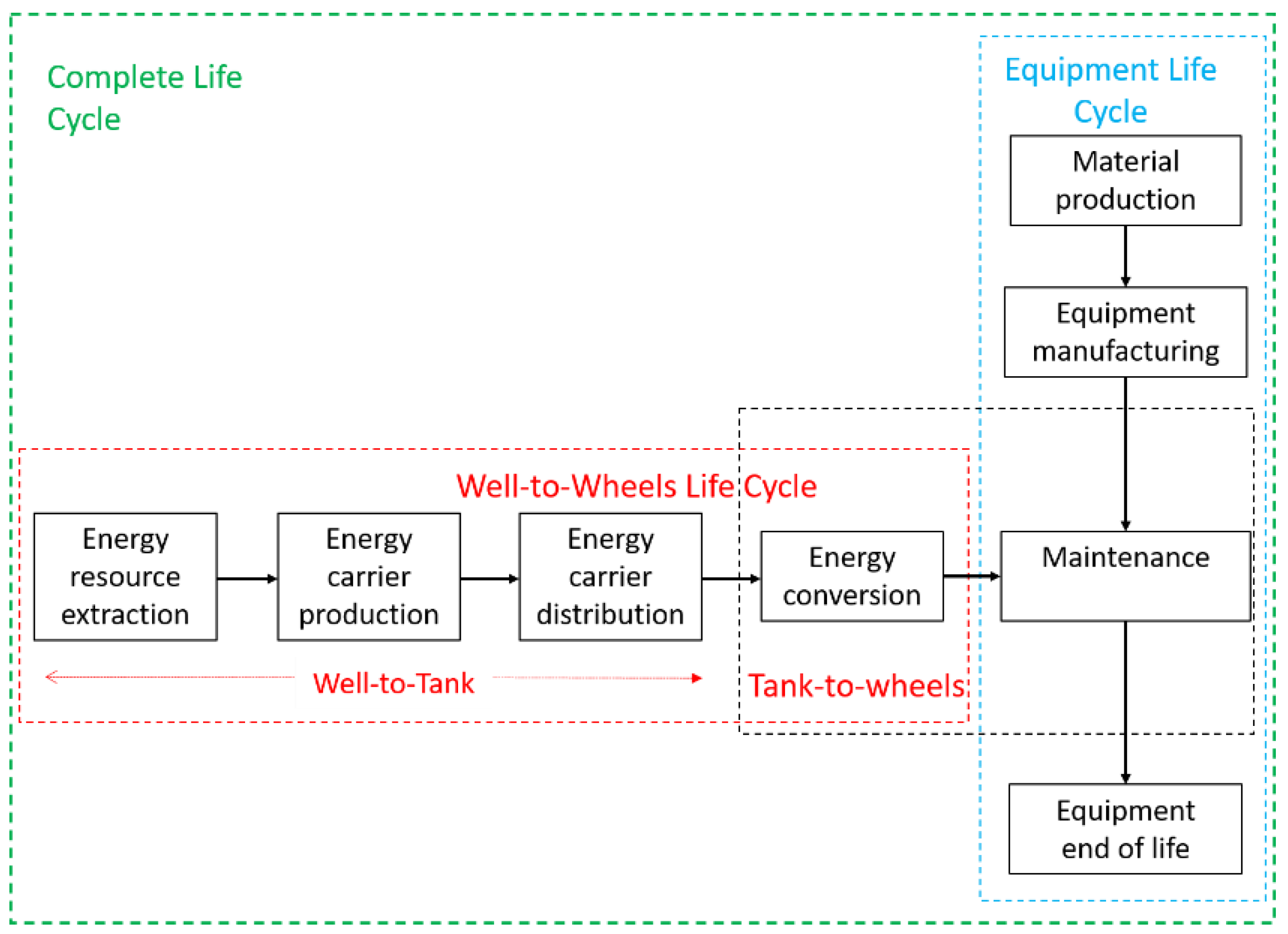
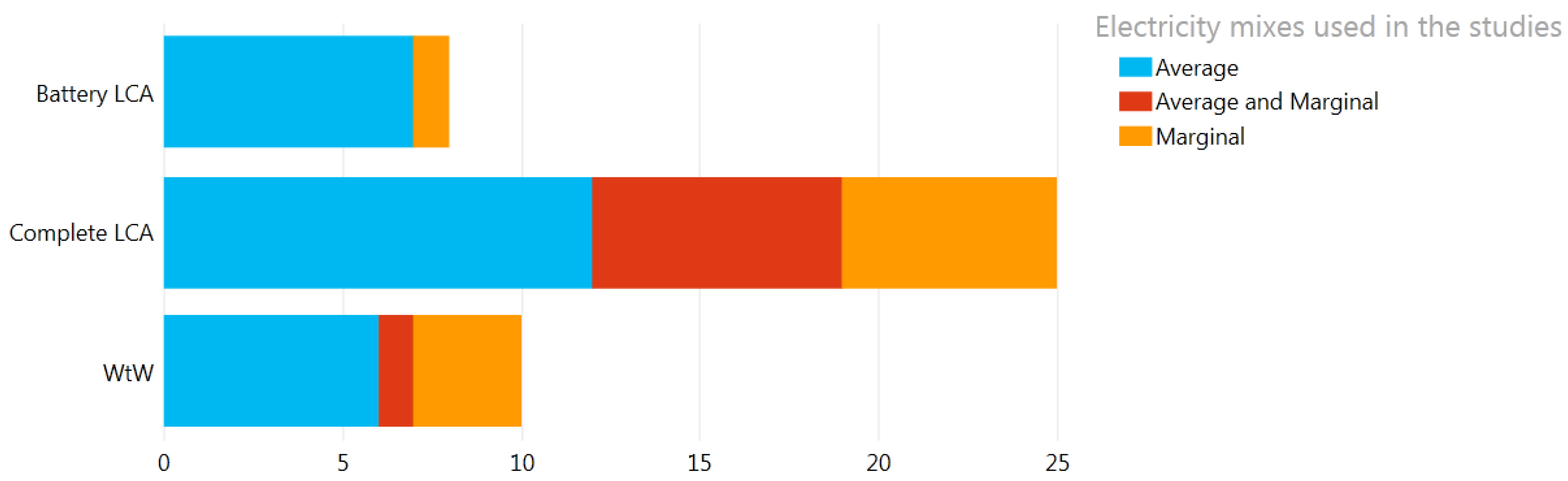
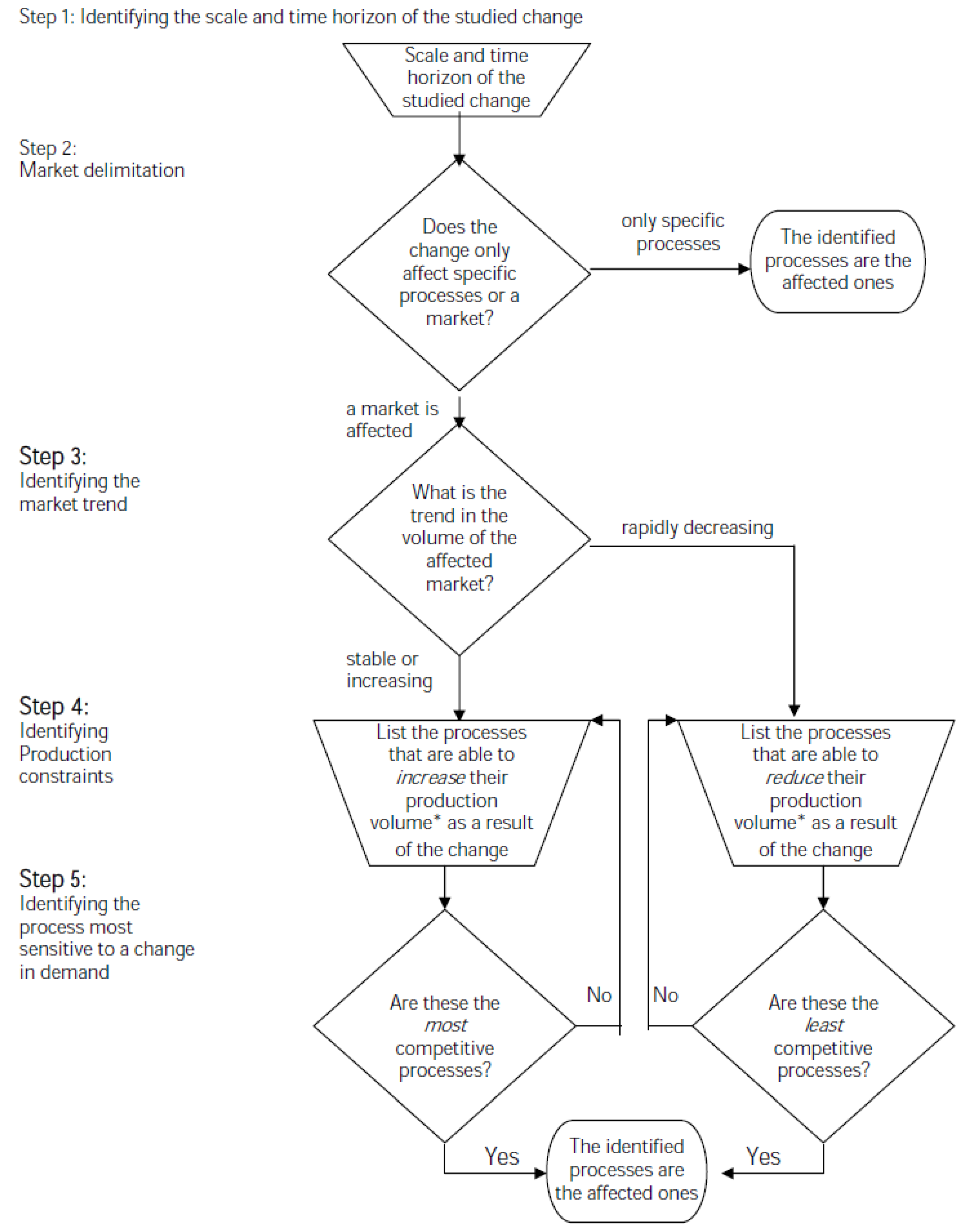
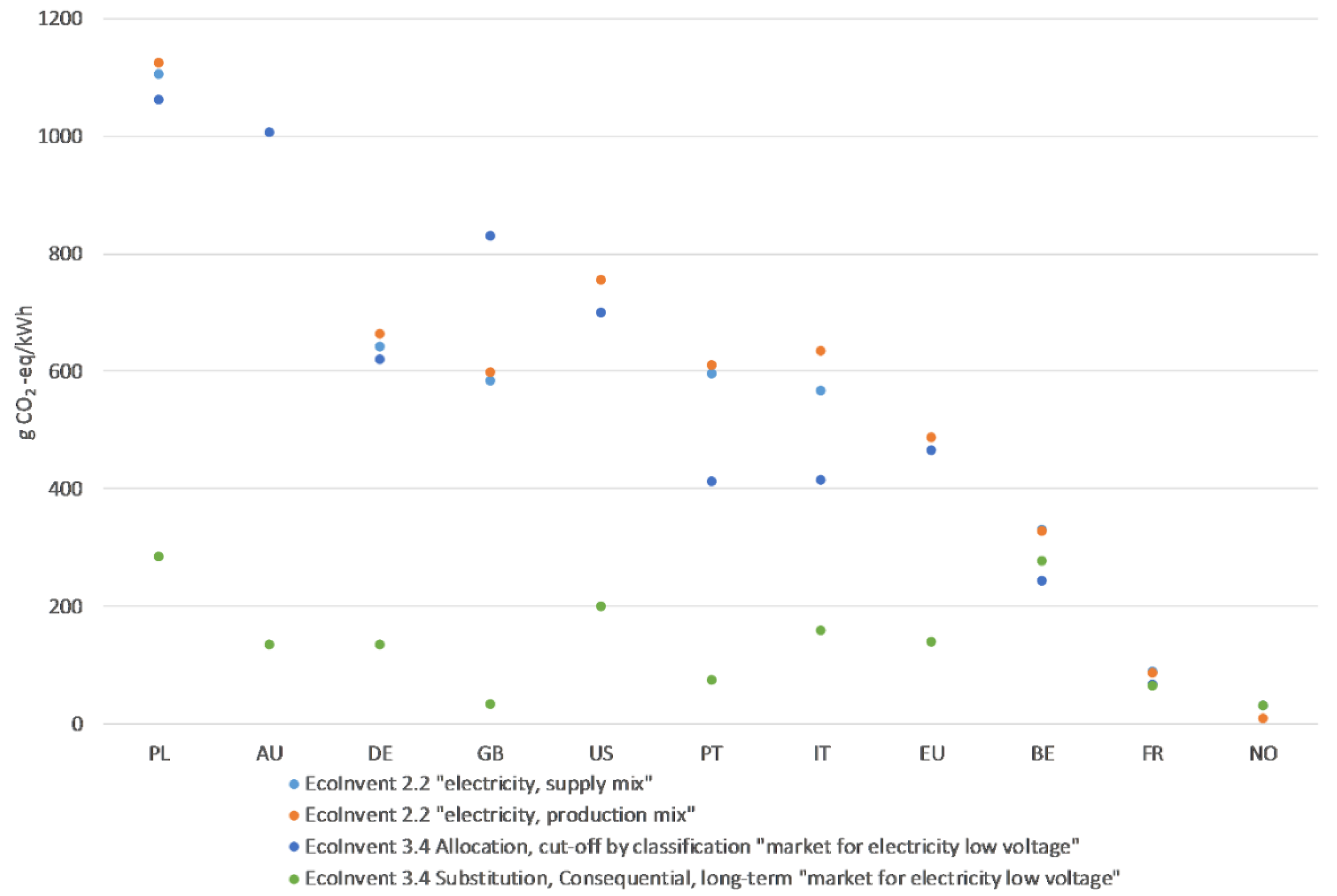
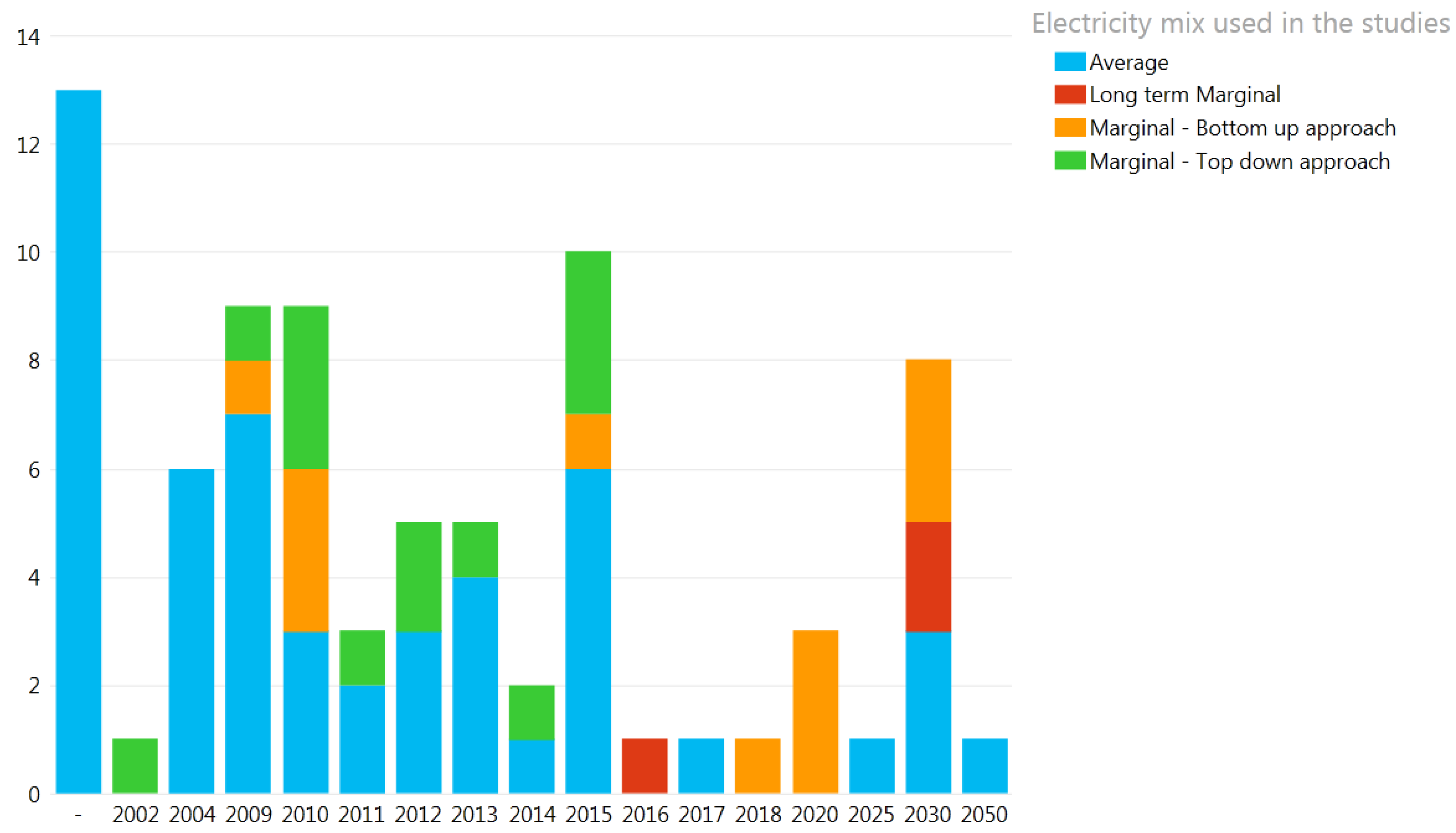
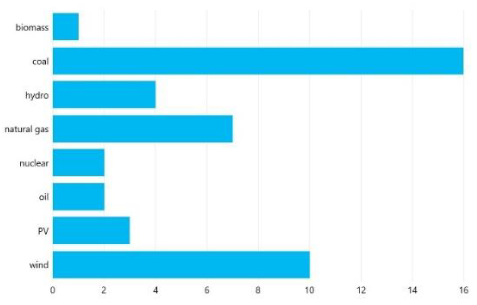
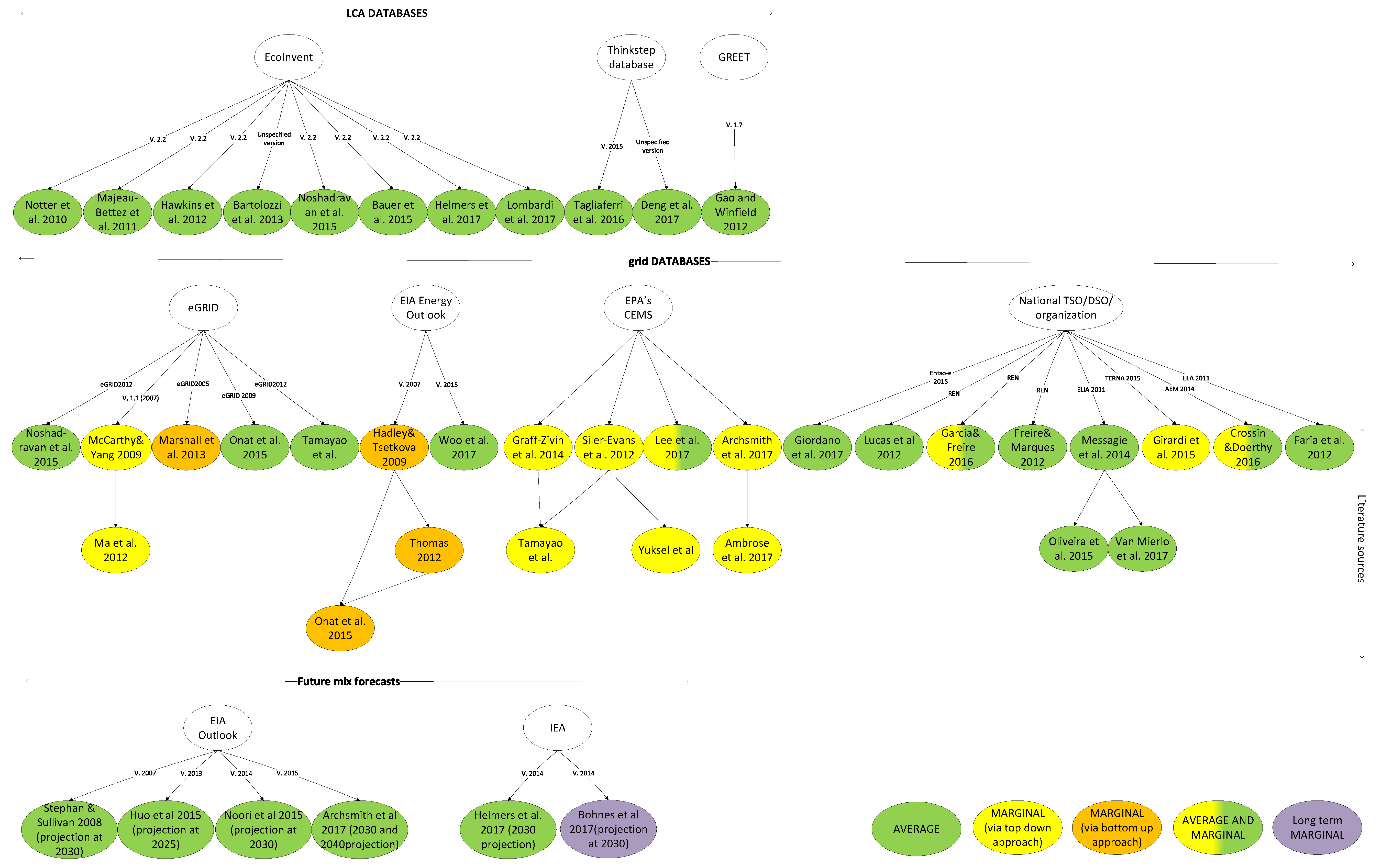
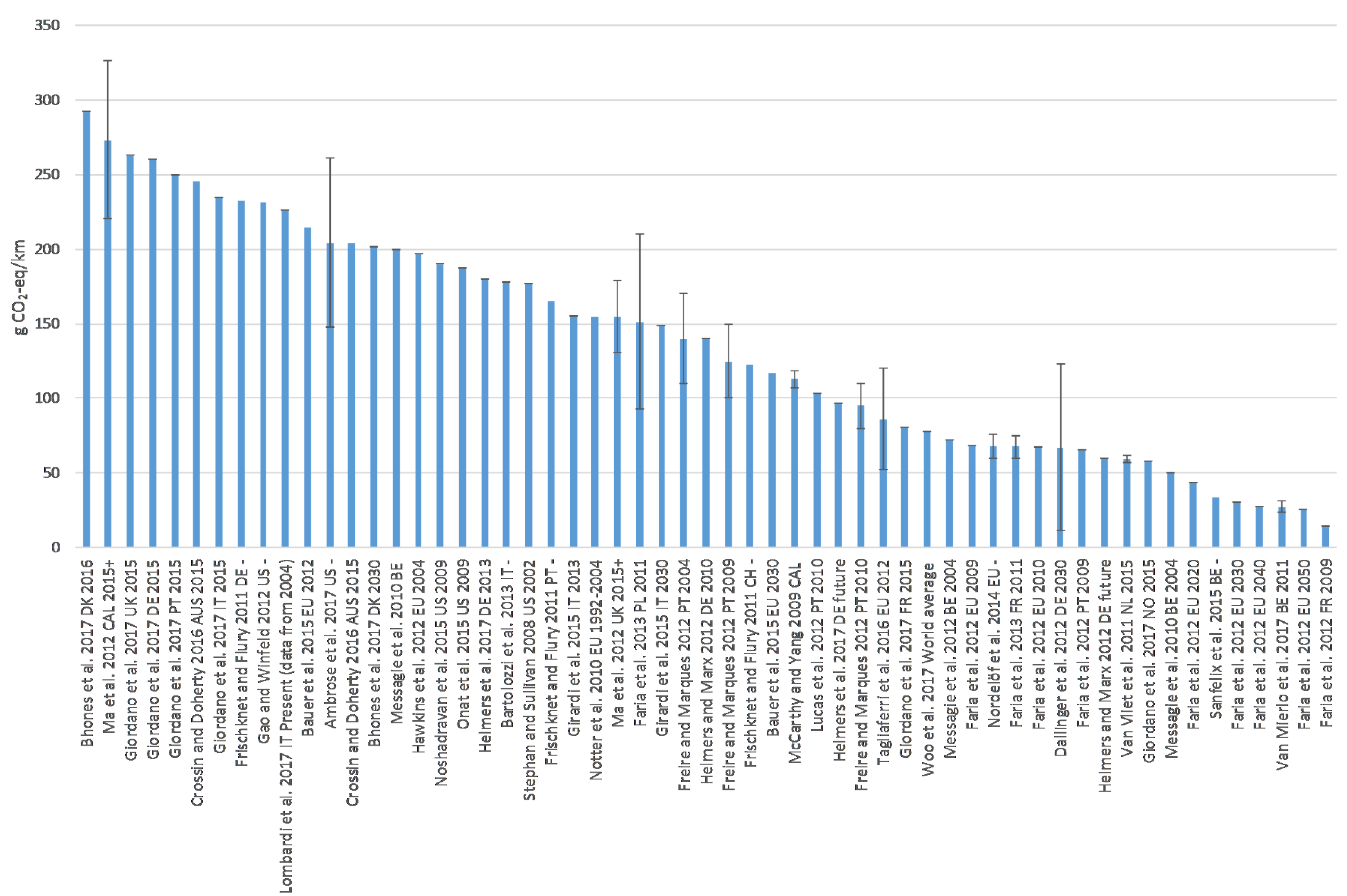
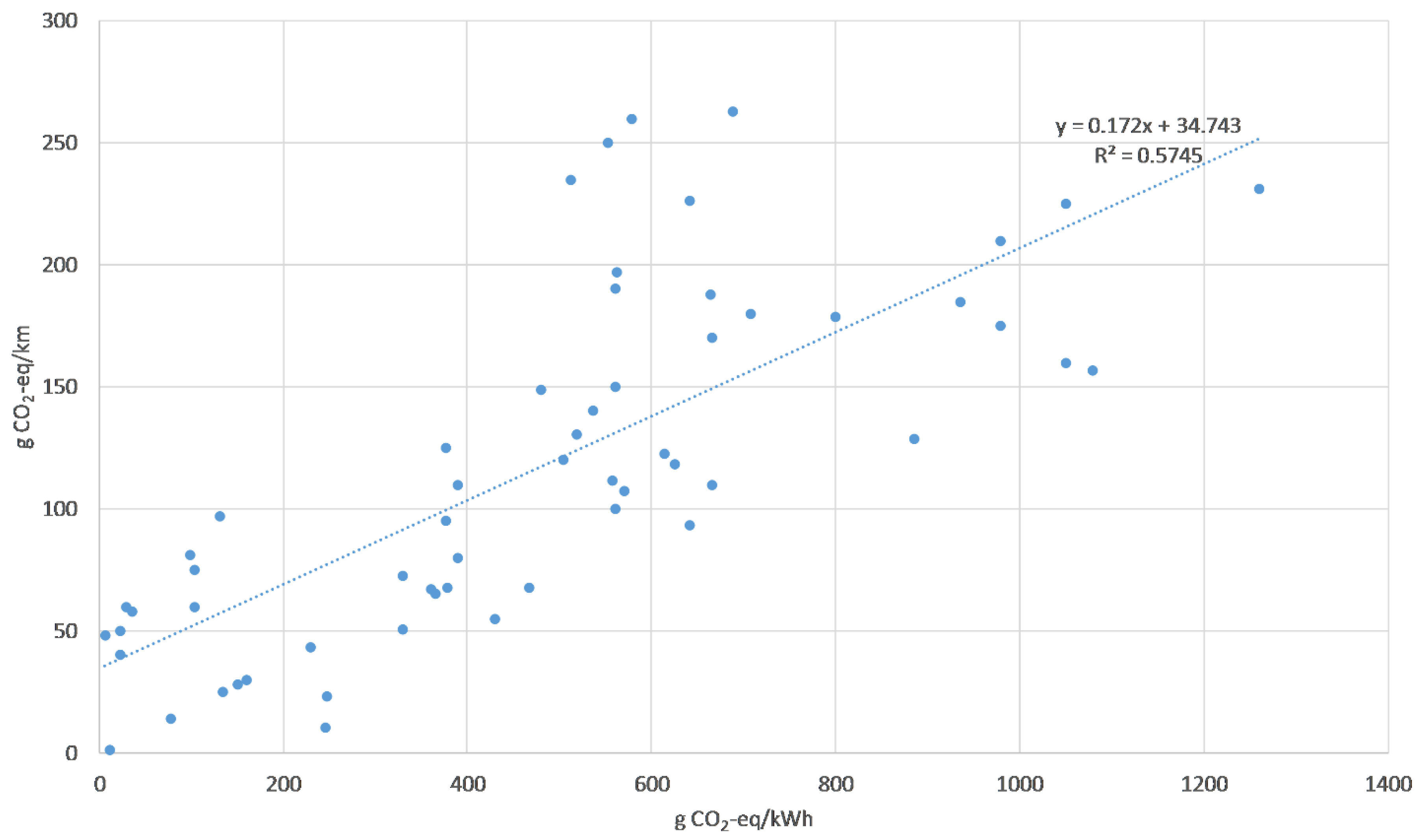
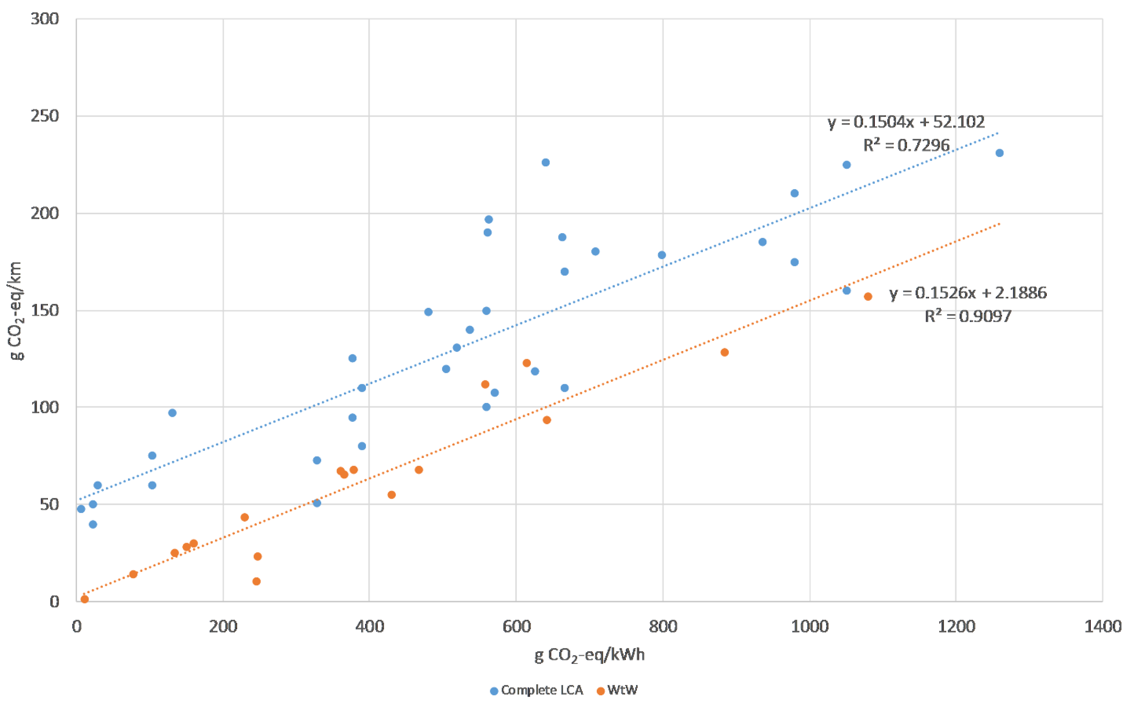
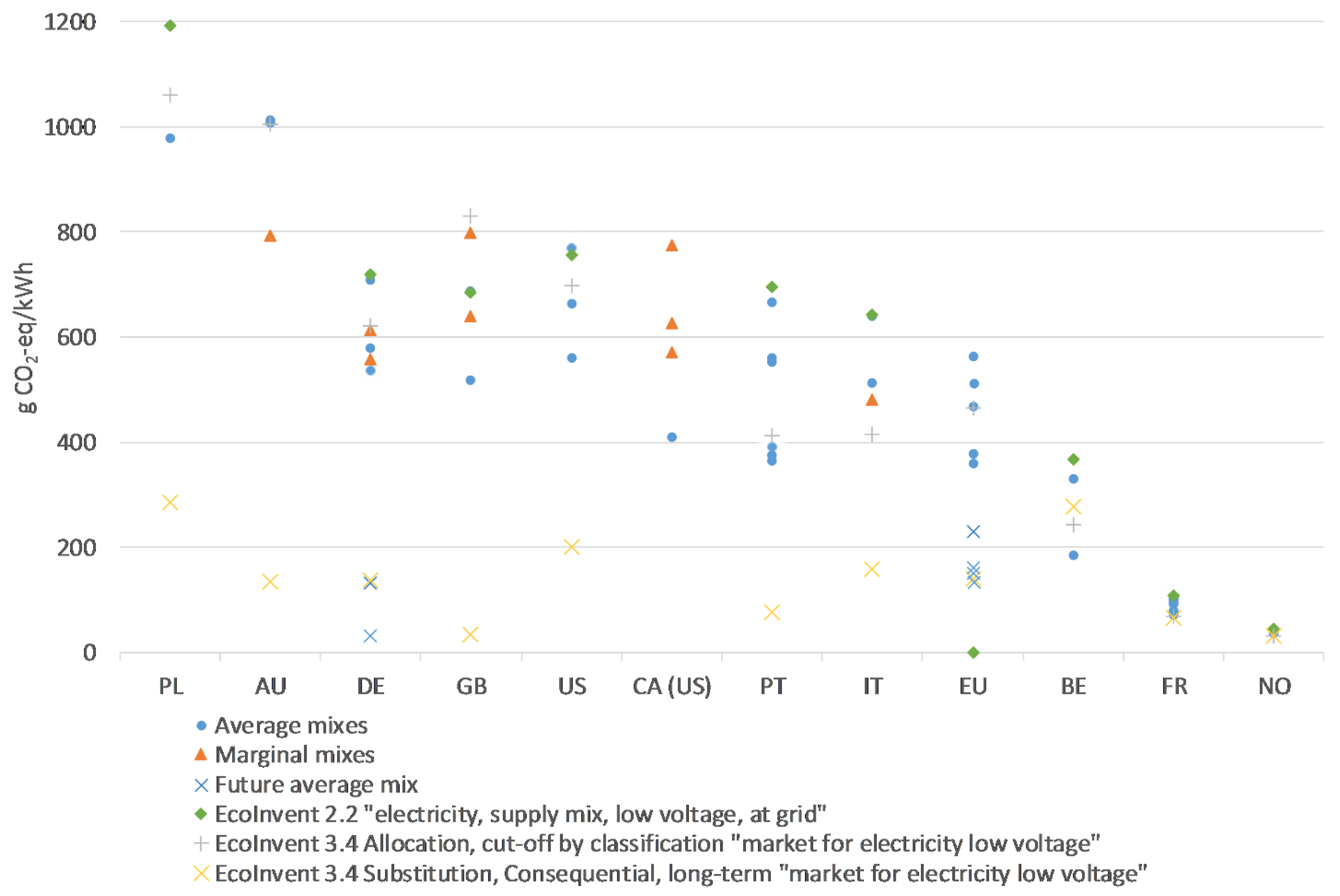
Table 1.
Synoptic view of the literature review.
| Authors | Region | Time Horizon | Penetration Rate | Vehicle | Electricity mix | BEV Impact (GHG) | |||
|---|---|---|---|---|---|---|---|---|---|
| Average | Marginal | Source | GHG Intensity | ||||||
| Complete LCA | |||||||||
| Archsmith et al., 2017 [22] | US NERC regions | 2011–2012 | - | ICEV, EV | a | EPA’s Continuous Emissions Monitoring Systems (CEMS); GREETnet | 513–1258 g CO2-eq/kWh | 4.22–6.11 ton CO2eq/vehicle/year (rebound effect included) (average 5.22) | |
| 2030 2040 | x | EIA forecasts | - | - | |||||
| Bartolozzi et al., 2013 [14] | Italy | - | - | BEV, ICHE, FC LCV (Piaggio Porter) | x | - | EcoInvent (unspecified version) | - | 178.25 g CO2-eq/km |
| Bauer et al., 2015 [23] | Switzerland (EU 27 mix in use phase) | 2012 | - | ICEV, HEV, Plug-in Hybrid (PHEV), BEV, FCV, FCHEV | x | EcoInvent v. 2.2 | - | 214 g CO2-eq/km EU electricity mix (BEV mid size, average efficiency 0.77 mj/km) | |
| 2030 | x | Kannan and Turton [24] and ESU-services/IFEU 2008 | - | 117 g CO2-eq/km EU mix (BEV mid size, average efficiency 0.64 mj/km) | |||||
| Bohnes et al., 2013 [20] | Denmark | From 2016 to 2030 | - | ICV, BEV, HEV, PHEV, nPHEV, REEV, FCEV fleet analysis | d | EcoInvent 3.1 Substitution, consequential updated with EU and DK projections | - | From 292 g CO2-eq/km in 2016 to 202 g CO2-eq/km in 2030 | |
| Crossin and Doherty 2016 [25] | Australia | 2015 | - | PHEV, ICEV | x | Australian Energy market operator | 1006 g CO2-eq/kWh | 246 g CO2-eq/km | |
| a | 794 g CO2-eq/kWh | 204 g CO2-eq/km | |||||||
| Faria et al., 2013 [26] | Poland | 2011 | - | gasoline and diesel ICEVs, PHEVs, BEVs, FCEVs | x | European Environment Aagency (EEA) 2011 | 979 g CO2-eq/kWh | 210 g CO2-eq/km (compact)” 175 g CO2-eq/km (subcompact peugeot iOn)” | |
| Portugal | 376 g CO2-eq/kWh | 125 g CO2-eq/km (compact)” 95 g CO2-eq/km (subcompact peugeot iOn)” | |||||||
| France | 103 g CO2-eq/kWh | 75 g CO2-eq/km (compact)” 60 g CO2-eq/km (subcompact peugeot iOn)” | |||||||
| Freire and Marques 2012 [27] | Portugal | 2004 | - | BEV, PHEV, gasoline, Diesel (compact and subcompact passenger vehicles) | x | REN | 666 g CO2-eq/kWh | 170 g CO2-eq/km (compact) 110 g CO2-eq/km (subcompact) | |
| 2009 | 560 g CO2-eq/kWh | 150 g CO2-eq/km (compact) 100 g CO2-eq/km (subcompact) | |||||||
| 2010 | 390 g CO2-eq/kWh | 110 g CO2-eq/km (compact) 80 g CO2-eq/km (subcompact) | |||||||
| Garcia and Freire 2016 [28] | Portugal | 2015–2017 | 35–59 GWh in 2017 | BEV | x | REN | 352 g CO2-eq/kWh | 352 g CO2-eq/km | |
| a | 723 g CO2-eq/km | ||||||||
| Girardi et al., 2015 [9] | Italy | 2013 (data from 2012) | “few EVs” | EV, ICEV | a | TRENA | 155 g CO2-eq/km (vehicle efficiency 0.19 kWh/km) | ||
| 2030 | +17.5 TWh | c(b) | Lanati et al. [29] | 480 g CO2-eq/kWh | 148.88 g CO2-eq/km (vehicle efficiency 0.19 kWh/km) | ||||
| Hawkins et al., 2012 [1] | EU | - | - | EV Li-NCM, EV LifePO4, ICEV diesel, ICEV gasoline | x | EcoInvent v. 2.2 | 562 g CO2-eq/kWh EU mix* | 196.79 g CO2-eq/km (0.713 kWh/km) | |
| Helmers et al., 2017 [16] | Germany | Present (data 2004) | - | BEV, ICEV, FCV new ICEV Smart, new e-Smart, Smart converted from combustion engine to electric; BEV, ICEV, FCV | x | EcoInvent v. 2.2 | 719.5 g CO2-eq/kWh | - | |
| 2013 | IEA | 707.4 g CO2-eq/kWh | 180 g CO2-eq/km | ||||||
| Generic future based on renewables | Nitsch et al., 2012 [30] | 130.6 g CO2-eq/kWh | 97 g CO2-eq/km | ||||||
| Helmers and Marx 2012 [17] | Germany | 2010 | - | BEV, ICEV, FCV smart: ICEV, e-SMART; BEV, ICEV, FCV | x | German federal environmental agency | 536 g CO2-eq/kWh | 140 g CO2-eq/km | |
| Lee et al., 2017 [10] | US states | 2014 | - | medium duty TRUCK diesel, biodiesel, biodiesel hybrid, CNG, CNG hybrid, electric) | x | EPA’s CEM hourly data and NEI database | - | - | |
| a | - | - | |||||||
| Lucas et al., 2012 [31] | Portugal | 2010 | - | gasoline, diesel, FCHEV, FCPHEV, EV | x | REN | - | 61 g CO2-eq/km | |
| Ma et al., 2012 [32] | UK | 2015+ (data from 2009–2010) | - | ICEV, HEV, BEV Mid size in UK | x | BM report | 518.4 g CO2-eq/kWh | 130.6 g CO2-eq/km | |
| a | 799.2 g CO2-eq/kWh | 178.7 g CO2-eq/km | |||||||
| California | 2015+ (data from 2010) | SUV in California; | x | McCarthy and Yang 2009 [33] | - | 220.4 g CO2-eq/km | |||
| c(b) | - | 326.6 g CO2-eq/km | |||||||
| McCarthy and Yang 2009 [33] | California | 2010 | 1% of VMT | ICEV, HEV, PHEV, BEV, FCV | x | eGRID v.1.1 (2007) | 250 g CO2-eq/kWh | ||
| b | 626 g CO2-eq/kWh (off peak marginal) 571 g CO2-eq/kWh (load level marginal) | 118.32 g CO2-eq/km (WTW) 107.44 g CO2-eq/km (WTW) | |||||||
| Marshall et al., 2013 [34] | Michigan | 2009 | 10% infiltration, additional 2.41 × 10¹⁰ MJ | mid size PHEV | b | - | - | 547–611 g CO2-eq/km (PHEV, efficiency 0.45 kWh/km) | |
| Noshadravan et al., 2015 [35] | US | 2009 | - | EV, ICEV | 227.1–894.2 g CO2-eq/kWh 560.65 g CO2-eq/kWh | 190 g CO2-eq/km” | |||
| Messagie et al., 2015 [36] | Belgium | 2012 2013 2017 | - | x | ELIA (Belgian DSO) | - | - | ||
| Onat et al., 2015 [37] | US states | 2009 | - | mid size BEV, ICEV, PHEV, HEV | x | eGrid | 663.4 g CO2-eq/kWh | 187.72 g CO2-eq/km | |
| 2020 | c (b) | Hadley and Tsvetkova [38] | range 644–911 g CO2-eq/kWh | ||||||
| Stephan and Sullivan 2008 [39] | US regions | 2002 | “a significant number” | PHEV | x | EPA | 608.4 g CO2-eq/kWh’ | 177 g CO2/km (PHEV, efficiency 0.92 MJ/km) (WTW) | |
| 2002 | a | ||||||||
| 2030 | d | 157 g CO2-eq/km | |||||||
| Van Mierlo et al., 2017 [40] | Belgium | 2011 | - | BEV, Compressed Natural Gas (CNG), Liquid Petrol Gas (LPG), Biogas (BG), PHEV, HEV | x | Messagie et al., 2014 [41] | 190 g CO2-eq/kWh | 31–24 g CO2-eq/km (wtw) | |
| Weis et al., 2016 [42] | US PJM | 2010 2018 | - | EV, HEV and conventional gasoline | b | UCED model (data from NEEDS database and EPA projections) | - | - | |
| Yuksel et al., 2016 [43] | US states | 2011 | - | 2013 Nissan Leaf BEV; 2013 Chevrolet Volt PHEV; 2013 Toyota Prius PHEV; Toyota Prius HEV; the Mazda 3 | c (a) | Siler-Evans et al. [44] | 430–932 kg CO2-eq/MWh | - | |
| Giordano et al., 2017 [15] | UK | 2015 | - | light duty vehicle (IVECO daily) BEV, diesel | x | EcoInvent 3.0 updated with data for 2015 from Entso-e | 688 g CO2-eq/kWh | 263 g CO2-eq/km, ni-nacl2 battery 2015 bev | |
| Germany | 579 g CO2-eq/kWh | 260 g CO2-eq/km, ni-nacl2 battery 2015 bev | |||||||
| Portugal | 553 g CO2-eq/kWh | 250 g CO2-eq/km, ni-nacl2 battery 2015 bev | |||||||
| Italy | 512 g CO2-eq/kWh | 235 g CO2-eq/km, ni-nacl2 battery 2015 bev | |||||||
| France | 98 g CO2-eq/kWh | 81 g CO2-eq/km, ni-nacl2 battery 2015 bev | |||||||
| Norway | 36. g CO2-eq/kWh | 58 g CO2-eq/km, ni-nacl2 battery 2015 bev | |||||||
| Lombardi et al., 2017 [18] | Italy | Present (data 2004) | - | gasoline ICEV, EV, gasoline PHEV, PHFCV | x | EcoInvent v. 2.2 | 640.8 g CO2-eq/kWh | 226 g CO2-eq/km | |
| USA | 770.4 g CO2-eq/kWh | - | |||||||
| France | 93.6 g CO2-eq/kWh | - | |||||||
| Tagliaferri et al., 2016 [45] | EU | 2012 | - | BEV (Nissan Leaf), ICEV (Toyota Yaris); PHEV | x | EcoInvent v. 2.2 | - | 120 g CO2-eq/km (Nissan leaf EVI 0.50 MJ/km)111 g CO2-eq/km (Nissan leaf EVII 0.50 MJ/km) | |
| 2050 | Behrens et al., 2013 (2050) | - | - | ||||||
| Tamayao et al., 2015 [46] | US regions | 2009 | - | PHEV (Chevrolet Volt), HEV (Toyota Prius), BEV (Nissan Leaf) | x | ANL | - | - | |
| a | Siler-Evans et al., 2012 [44] Graff Zivin et al., 2014 [3] | - | - | ||||||
| W-t-W Analysis | |||||||||
| Thomas 2012 [47] | US electrical power regions | 2020 | - | HEV, PHEV, BEV | c (b) | Hadley and Tsvetkova [38] | - | - | |
| Dallinger et al., 2012 [48] | Germany | 2030 | 12 milion EV | BEV | b | own calculation Elgowainy et al., 2010 [4] | 247.26 construction and dispatch of RES to serve EVs 245.42 construction and dispatch of RES to serve EVs614 long term high RES mix (2030) 558.21 long term high RES mix (2030) | 23.4 g CO2-eq/km last trip charging; 10.7 g CO2-eq/km DSM charging; 122.84 g CO2-eq/km DSM charging; least marginal cost dispatch 111.64 g CO2-eq/km last trip charging; least marginal cost dispatch | |
| Van Vliet et al., 2011 [49] | Nederland | 2015 | - | SHEV, BEV, PHEV, gasoline, diesel | b | Van den Broek et al. [50] | - | 62 g CO2-eq/km (uncoordinated charging) 57 g CO2-eq/km (off-peak charging) | |
| Faria et al., 2012 [51] | Portugal | 2009 | - | ICE, HEV, PHEV, BEV, future BEV | x | - | Eea Eurostat | 365 g CO2-eq/kWh | 65.3 g CO2-eq/km’ |
| France | 78 g CO2-eq/kWh | 14 g CO2-eq/km’ | |||||||
| EU | 2009 | 378 g CO2-eq/kWh | 68 g CO2-eq/km’ | ||||||
| 2010 | 360 g CO2-eq/kWh | 67.3 g CO2-eq/km’ | |||||||
| 2020 | 230 g CO2-eq/kWh | 43.3 g CO2-eq/km’ | |||||||
| 2030 | 160 g CO2-eq/kWh | 30 g CO2-eq/km’ | |||||||
| 2040 | 150 g CO2-eq/kWh | 28 g CO2-eq/km’ | |||||||
| 2050 | 135 g CO2-eq/kWh | 25.3 g CO2-eq/km’ | |||||||
| Woo et al. 2017 [52] | 70 countries | 2014 | - | EV, ICEV | x | - | IEA (2015b), EIA (2015) World Bank (2016) | - | 78.1 g CO2-eq/km (world average) |
| Huo et al., 2015 [13] | US (3 regions), China (3 regions) | 2012 | EV, PHEV, ICEV | x | - | 190–290 g CO2-eq/km’ “(China), 110–225 (US) g CO2-eq/km’ “ | |||
| 2025 | EIA (2015) | - | 110–160 g CO2-eq/km’ “ (China), 60–150 (US) g CO2-eq/km’ “ | ||||||
| Gao and Winfeld 2012 [53] | US | CV (Toyota Corolla), HEV(Prius), PHEV (Prius Plug-in), EREV (GM Volt), EV (Nissan Leaf), FCV (Honda Clarity) | x | GREET | - | 240 g CO2-eq/km“ (efficiency 0.213 kWh/km) | |||
| Battery LCA | |||||||||
| Ambrose et al., 2016 [54] | US states | see Archsmith | - | c(a) | Archsmith et al. [22] | - | - | ||
| Majeau-Bettez et al., 2011 [7] | EU | - | x | EcoInvent v. 2.2 | - | - | |||
| Deng et al., 2017 [55] | US | - | x | Thinkstep (unspecified version) | - | - | |||
| Zackrisson et al., 2010 [56] | West Europe, Scandinavia, China | - | x | - | - | ||||
| Garcia et al., 2017 [12] | EU-27 France | - | x | - | - | ||||
| Oliveira et al., 2015 [57] | Belgium (EU mix) | 2011 (data from 2004) | - | x | 516 g CO2-eq/kWh | - | |||
| Sanfelix et al., 2015 [58] | EU | - | x | 33.9 g CO2-eq/km (WtW 25.7 g CO2-eq/km) | |||||
| Notter et al., 2010 [6] | EU | - | BEV golf class | x | EcoInvent v. 2.01 | 592.61 g CO2-eq/kWh | 155 g CO2-eq/km (vehicle efficiency 0.17 kWh/km including auxiliary energy consumption) | ||
| Eco balance | |||||||||
| Noori et al., 2015 [11] | US electric regions | 2030 | - | ICEV, gasoline HEV, gasoline PHEV, gasoline EREV, BEV | b | EIA projections | - | - | |
| LCA of energy-demanding products | |||||||||
| Roux et al., 2017 [59] | France | reference year (averaging annual economic and meteorological variations) | x | RTE | 61.4 to 84.9 g CO2eq/kWh of heating in households | ||||
| b | 765.1 to 928.7 g CO2eq/kWh of heating in households | ||||||||
| Alvarez Gaitan et al., 2014 [60] | Australia | 2030 | +1 Mg of NaClO and1Mg FeCl3 | b, d | |||||
| Colett et al. [61] | US (different boundary levels) | 2010 | nested approach | 19.0 and 19.9 kg CO2-eq/kg primary aluminium ingot | |||||
* Value obtained a posteriori looking for the EcoInvent dataset “Electricity production mix low voltage RER” (IPCC 2007 100a); “value normalised by the author“; value inferred from bar graph; a = marginal mix obtained through bottom up approach; b = marginal mix obtained through top down approach; c() = marginal mix obtained from the literature; d = long term marginal.
Table 2.
Combination of two main aspects of the decision-context: Decision orientation and kind of consequences in background system or other systems [19]. (Reproduced with permission from [19], Publications Office of the European Union, 2014)
| Decision support? | Kind of Process-Changes in Background System/Other Systems | ||
| Yes | None or small-scale | Large-scale | |
| Situation A “Micro-level decision support” | Situation B “Meso/macro-level decision support” | ||
| No | Situation C “Accounting” (with C1: Including with other systems, C2: Excluding interactions with other systems) | ||
Table 3.
Energy GHG intensity and GHG of BEV in stylised states across the literature.
| Stylised State | g CO2-eq/kWh | g CO2-eq/km | |
|---|---|---|---|
| Bartolozzi et al. [14] | Biomass | - | 110.35 |
| Nordelöf et al., 2014 [2] | CNG | 642 | 93.5 (WtW) |
| Van Mierlo et al., 2017 [40] | CNG | - | 93.5 (WtW) |
| Giordano et al., 2017 [15] | Coal | 1180 | 482 |
| Nordelöf et al., 2014 [2] | Coal | 1080 | 157 (WtW) |
| Stephan and Sullivan 2008 [39] | Coal | 954 | 274 (WtW, PHEV) |
| Van Mierlo et al., 2017 [40] | Coal | - | 157 (WtW) |
| Bauer et al., 2015 [23] | Coal (average efficiency in 2012) | - | 371 |
| Bauer et al., 2015 [23] | Coal (average efficiency in 2030) | - | 308 |
| Freire and Marques 2012 [27] | Coal (desulfurisation and denitrification | 1050 | 225 (Compact BEV) 160 (Subcompact BEV) |
| Hawkins et al., 2012 [1] | Coal (EcoInvent Dataset) | 1260 | 231 |
| Hawkins et al., 2012 [1] | Coal IGCC | 936 | 185 |
| Hawkins et al., 2012 [1] | Hydro | 6.12 | 48 |
| Stephan and Sullivan 2008 [39] | Hydro | 0 | 0 (WtW, PHEV) |
| Bauer et al., 2015 [23] | Hydro (average efficiency in 2012) | - | 66.9 |
| Bauer et al., 2015 [23] | Hydro (average efficiency in 2030) | - | 55.8 |
| Dallinger et al. [48] | Marginal mix in a scenario with dedicated RES for additional EV loads | 247.26 (last trip charging) | 23.4 (WtW) |
| 245.42 (DSM charging) | 10.7 (WtW) | ||
| Stephan and Sullivan 2008 [39] | Natural gas | - | 184 (WtW, PHEV) |
| Bauer et al., 2015 [23] | Natural gas (average efficiency in 2012) | - | 186 |
| Bauer et al., 2015 [23] | Natural gas (average efficiency in 2030) | - | 155 |
| Hawkins et al., 2012 [1] | NGCC | 504 | 120 |
| Van Vliet 2011 [49] | NGCC | 430 | 55 (WtW) |
| Bauer et al., 2015 [23] | Nuclear (average efficiency in 2012) | - | 68 |
| Bauer et al., 2015 [23] | Nuclear (average efficiency in 2030) | - | 56.7 |
| Nordelöf et al., 2014 [2] | Oil | 885 | 128.5 (WtW) |
| Stephan and Sullivan 2008 [39] | Oil | 892.8 | 262 (WtW, PHEV) |
| Oliveira et al., 2015 [57] | PV | 89 | - |
| Bauer et al., 2015 [23] | PV (average efficiency in 2012) | - | 87.2 |
| Bauer et al., 2015 [23] | PV (average efficiency in 2030) | - | 72.6 |
| Bartolozzi et al. [14] | Wind | - | 121.2 |
| Freire and Marques 2012 [27] | Wind | 23 | 50 (Compact BEV) 40 (Subcompact BEV) |
| Nordelöf et al., 2014 [2] | Wind | 11 | 1.50 (WtW) |
| Oliveira et al., 2015 [57] | Wind | 11.2 | - |
| Van Mierlo et al., 2017 [40] | Wind | - | 1.50 (WtW) |
| Crossin and Doherty 2016 [25] | Wind | 24 | 76 |
| Bauer et al., 2015 [23] | Wind (average efficiency in 2012) | - | 70.4 |
| Bauer et al., 2015 [23] | Wind (average efficiency in 2030) | - | 58.7 |
© 2018 by the authors. Licensee MDPI, Basel, Switzerland. This article is an open access article distributed under the terms and conditions of the Creative Commons Attribution (CC BY) license (http://creativecommons.org/licenses/by/4.0/).
Share and Cite
MDPI and ACS Style
Marmiroli, B.; Messagie, M.; Dotelli, G.; Van Mierlo, J. Electricity Generation in LCA of Electric Vehicles: A Review. Appl. Sci. 2018, 8, 1384. https://doi.org/10.3390/app8081384
AMA Style
Marmiroli B, Messagie M, Dotelli G, Van Mierlo J. Electricity Generation in LCA of Electric Vehicles: A Review. Applied Sciences. 2018; 8(8):1384. https://doi.org/10.3390/app8081384
Chicago/Turabian StyleMarmiroli, Benedetta, Maarten Messagie, Giovanni Dotelli, and Joeri Van Mierlo. 2018. "Electricity Generation in LCA of Electric Vehicles: A Review" Applied Sciences 8, no. 8: 1384. https://doi.org/10.3390/app8081384
Note that from the first issue of 2016, this journal uses article numbers instead of page numbers. See further details here.