A New Method for Active Cancellation of Engine Order Noise in a Passenger Car


Acoustics and Vibration Signal Processing Lab., Department of Mechanical Engineering, Inha University, Incheon 22201, Korea
*
Author to whom correspondence should be addressed.
Appl. Sci. 2018, 8(8), 1394; https://doi.org/10.3390/app8081394
Submission received: 8 June 2018
/
Revised: 3 August 2018
/
Accepted: 14 August 2018
/
Published: 17 August 2018
(This article belongs to the Special Issue Active and Passive Noise Control)
Abstract
:Featured Application
The proposed framework is highly suitable for audio applications for active sound noise cancellation and active sound design in a vehicle.
Abstract
This paper presents a novel active noise cancellation (ANC) method to reduce the engine noise inside the cabin of a car. During the last three decades, many methods have been developed for the active control of a quasi-stationary narrowband sinusoidal signal. However, since the interior noise signal is non-stationary with a fast frequency variation when the car accelerates rapidly, these methods cannot stably reduce the interior noise. The proposed method can reduce the interior noise stably even if the speed of the car is changed quickly. The method uses an adaptive filter with an optimal weight vector for the active control of such an engine noise. The method of determining the optimal weight vector of an adaptive filter is demonstrated. In order to validate the advantages of the proposed method, a conventional method and the proposed method are simulated with three synthesized signals. Finally, the proposed method is applied to the cancellation of booming noise in a sport utility vehicle. We demonstrate that the performance of the ANC system with the proposed algorithm is excellent for the attenuation of engine noise inside the cabin of a car.
1. Introduction
While driving a passenger car, a driver can hear many types of sounds inside the car [1]. Among them, the engine is one of the dominant noise sources and influences the sound quality of the interior environment [2]. The frequency components of engine noise are correlated to the rotating speed of the crankshaft (i.e., rpm) of an engine and its harmonics [3]. These harmonic components are called ‘orders’. This correlation relationship between the engine noise and the rotating speed enables the control of the engine sound by using active control systems. Active noise control (ANC) has received considerable attention in recent decades, owing to its superior advantages in cancelling low frequency noise as compared to passive methods [4,5]. Adaptive feedforward control systems are very popular in active control systems (such as ANC) for the reduction of engine noise inside a car cabin [4,5,6,7]. This system uses an order signal as a reference. Order signals are sinusoidal signals within a narrow band, and can be synthesized by using the controller area network (CAN) bus (or a tachometer) in a car. The frequency of the order signal is changed in the run-up condition of the engine speed, and is a non-stationary signal. Many adaptive filters can be used in ANC systems [8]. In previous studies, the filtered x-LMS algorithm (FxLMS) based on the adaptive notch filter (ANF) has been widely used for the ANC of engine noise [7]. The filter length of the adaptive filter and the step-size should be carefully selected to ensure that the least mean squares (LMS) algorithm converges rapidly and is stable. Haykin [9] discussed the method to select the appropriate filter length and step size parameter. Although there are some implementations of variable length LMS adaptive filters, their performance is not steady [10]. Bilcu et al. introduced a variable LMS adaptive filter [11]. They suggested an implementation of multiple adaptive filters with variable lengths. Nascimento [12] proposed a method to speed up this convergence rate by varying the length of the adaptive filter, utilizing the larger step sizes allowed for short filters. These studies show the possibility of acquiring a rapid convergence when the optimal length of an adaptive filter is applied to the control of engine noise inside the cabin of a car. An adaptive notch filter used for the ANC of engine noise removes the primary spectral components within a narrowband centered at the frequency of reference. The filter length of the adaptive notch filter used in this study is short and two weights have been used.
The other inherent feature of the LMS algorithm is the step size, and it requires careful adjustment. A small step size, required for small excess mean square error, results in slow convergence. A large step size, required for fast adaptation, may result in the loss of stability. Therefore, many modifications of the LMS algorithm, where the step size changes during the adaptation process depending on particular characteristics, have been developed [9,13].
The performance of the adaptive notch filter depends heavily on the accuracy of the frequency of the reference signal because the bandwidth of the adaptive notch filter is proportional to the convergence step size [14,15]. The frequency change of the reference signal deteriorates the performance of an ANC system [16]. Therefore, in order to improve the convergence rate, the optimization of the step size in the adaptive notch filter is required for the ANC of engine noise [6]. Bismor [17] reviewed seventeen of the best-known variable step size LMS (VS-LMS) algorithms to the degree of detail that allows implementing them. The performance of the algorithms is compared in typical applications. According to the conclusion of this review, no VS-LMS algorithm appears to be as versatile, easy to use, and well-suited for real-time applications as the normalized least mean squares filter (NLMS). Recently, an NEX_LMS algorithm that uses the normalized signal as a reference has been proposed to improve the convergence rate for active sound quality control [18]. It improved the convergence rate of an ANC system using the Filtered-X LMS (FxLMS) algorithm, and achieved a large order-level reduction of the stationary disturbance of engine noise. An adaptive recursive algorithm has been proposed for the fast convergence of a controller in the ANC system of a short duct [19] for a non-stationary signal. In the present study, the optimized weights-FxLMS (OW-FxLMS) algorithm is proposed. Our goal is to control amplitude- and frequency-modulated noise, such as the order components of engine noise inside a car, with fast convergence. The performance of the algorithm is investigated with computer simulations and an experimental application in a car. The application purpose of this algorithm is to control the envelope of amplitude modulation signal and to generate the target sound with good sound quality inside of a car. The target sound is designed by the combination of the engine orders sound [20]. The sound quality of the target sound is determined by the sound quality index based on booming sound and modulation sound [21]. The booming sound and modulation sound were determined by the sound pressure level of the engine order sounds. Therefore, in order to design the amplitude of the target, the amplitude of the engine order sound should be controlled. The proposed optimized weights-FxLMS (OW-FxLMS) algorithm is suitable for this application. In Section 2, the novel OW-FxLMS algorithm is proposed. The utility of the proposed algorithm is validated in Section 3. The adaption for the proposed algorithm is explained in Section 4. The application of the algorithm to control of the interior noise is presented in Section 5. Finally, the conclusion is presented in Section 6.
2. Development of Novel Algorithm for Control of Amplitude of Order Sound
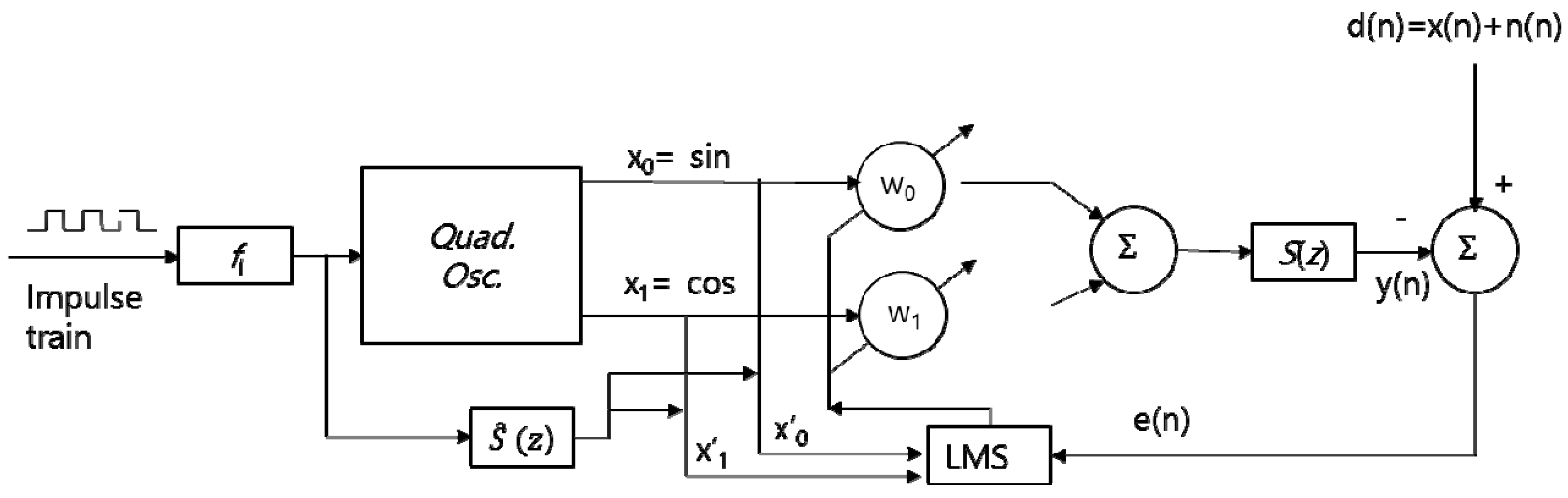
2.1. Conventional Method for ANC of Engine Noise
The FxLMS-algorithm-based adaptive notch filter has been used for the active noise cancellation of engine noise [4,5,22]. It is called the “conventional method” in the paper. The scheme of this ANC system is shown in Figure 1. This system uses two single sinusoidal reference signals, x0 and x1, and two single weights, w0 and w1, to control the engine noise. S(z) is the secondary path of the transfer function, and is the estimation of the secondary path. A suitable reference signal can be generated synthetically by measuring the current rotation speed fki of the engine and utilizing a discrete-time oscillator [23]. The primary disturbance d(n) comprises a multi-sinusoidal signal, which is the engine noise inside the cabin of a car. The multi-sinusoidal signal is correlated to the reference signals. In order to control the multi-sinusoidal signal, this scheme could be expanded to a multi-input/multi-output FxLMS control algorithm [6,7]. In the simplified single-frequency ANC system as shown in Figure 1, yk(n) is given by
The two weights w(n) of the adaptive filter are updated as
where μ is the step size controlling the stable convergence of the controller and is the filtered version of x(n) and is given by
where is an Mth-order estimate of the secondary path impulse response.
The adaptive notch filter removes the primary spectral components within a narrow band centered at the frequency fki (t) of the reference signal. The performance of the adaptive notch filter to cancel a sinusoidal signal depends heavily on the accuracy of the frequency of the reference signal [16] since the center frequency of the notch filter depends on the sinusoidal reference signal, whose frequency is equal to the frequency of the sinusoidal noise to be cancelled. The increment of step size μ results in a stability problem because, in an adaptive notch filter, the convergence step size is proportional to the bandwidth of the filter [9,15] and the higher the step size, the higher the bandwidth. Considering stability, the optimal step size is proposed [7] as follows:
where L is filter length of adaptive filter and A is the amplitude of the sinusoidal reference. The 3 dB bandwidth B of the notch filter can be estimated as
where ∆ is sampling time. From Equation (8), when the instantaneous frequency of the sinusoidal reference varies rapidly, the bandwidth B adaptive filter should be very narrow in order to track the time varying frequency and thus, the step size μ decreases. The small step size μ yields a slow convergence. The slow convergence cannot track the subsequent rapid varying frequency of the sinusoidal reference. Therefore, except for a quasi-stationary sweep of the instantaneous frequency of the sinusoidal reference, this system is not appropriate for controlling a frequency-modulated signal with a quickly variable bandwidth. Moreover, the performance of this ANC system is reduced when the run-up speed of the engine is changed rapidly [10,12]. Through further improvements, a new LMS algorithm based on the variable step size is proposed. Several variable step size strategies have been suggested to improve the performance of the LMS algorithm. These strategies enhance the performance of the algorithm, but a major drawback is the complexity in the theoretical analysis of the resultant algorithms [16]. According to conclusion of this review, most of the VS-LMS algorithms suggest a general modification that can simplify the choice of the upper bound for the step size. For the variable step size, the NLMS algorithm is employed and uses the following equation:
where a scalar that allows for a change of adaptive speed and is an estimate of the power of x(n) at time n. In order to further stabilize the digital implementation of the LMS algorithm, a technique known as leakage is used. In the leaky NLMS algorithm [9,14] the weight vector is updated by the following equation:
where γ is the leakage factor and satisfies the following condition for the leaky NLMS algorithm [24].
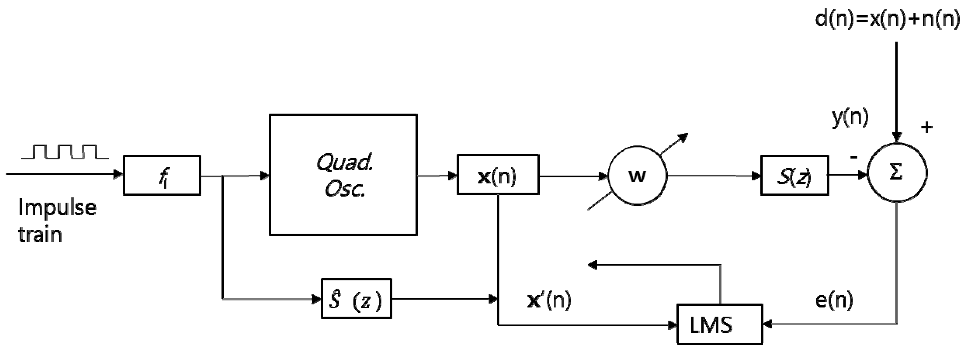
2.2. Novel Optimized Weights-LMS Algorithm: OW-FxLMS
We propose a new algorithm to improve the performance of the FxLMS algorithm to control an amplitude- and frequency-modulated signal such as an engine harmonic order signal.
The main objective the proposal algorithm is to control the amplitude of time varying engine order sounds with fast frequency change. In order to achieve this purpose, the design principles of the new ANC algorithm are that the frequency bandwidth of the adaptive filter should be wide and include the frequency of the engine order sound signal to be controlled by the adaptive filter. However, the limitation of this adaptive filter cannot control each order sound separately if frequencies of order sounds are too close, because the frequency bandwidth is wide. This is the limitation of the proposed algorithm. In order to overcome this limitation, the weighting of the adaptive filter should optimized. Therefore, in this section, the OW-FxLMS is proposed.
In order to trace a fast frequency change of the order sound signal, the optimized sufficient frequency bandwidth is required. The frequency bandwidth of an adaptive filter for tracking the frequency modulated signal is determined by the length of the weight vector [8,9,14]. The proposed algorithm is an FxLMS-algorithm-based adaptive filter with an optimal length of the weight vector wk (n). We determined the optimal length of the weight vector in order to trace a frequency-modulated signal such as an engine order signal. The frequency bandwidth between orders for rotating machinery is given by
where ∆k is the difference between the orders to be controlled. According to the theory of adaptive signal processing [9], the frequency bandwidth of an adaptive filter is given by where fs is the sampling frequency. The optimal frequency bandwidth fWB of an adaptive filter to be used by a controller should be less than the frequency bandwidth between the orders to be controlled by a controller. The adaptive filter is a moving bandpass filter with different center frequencies. The frequency bandwidth of the frequency-modulated signal to be cancelled should be less than the bandwidth of the adaptive filter in the proposed OW-FxLMS algorithm. Therefore, in the ANC system shown in Figure 2, yk (n) is given by
And the proposed OW-FxLMS algorithm is given by
where the length of weight vector is the optimal length L0. It is given by
The step size parameter μ should be carefully selected to ensure that the LMS algorithm converges rapidly and is stable. Haykin (9) proposed the condition to select the appropriate step size parameter as follows:
where Px denotes the power of x(n). From Equations (12) and (13), when the power of the reference signal changes, if Lo is changed, the step size μ should also be changed according to the convergence theory of the LMS algorithm. In practice [7], the relationship between step size and filter length for convergence is as follows:
When the input signal has varying frequency, the NLMS algorithm with variable step size should be used for further improvements. Therefore, the estimated power of x(n) at time n should be computed dynamically and thus, the variable step size is changed corresponding to Equation (6) because the optimal filter length Lo is constant. Finally, the pseudo code for the proposed OW-FxLMS algorithm is presented in Table 1.
3. Simulation and Validation of the Proposed Algorithm
3.1. Synthesizing the Engine Noise Signal Inside a Car Cabin
Engine noise is a periodic signal. From the theory of Fourier series expansion, a periodic signal (such as engine noise) can be decomposed into a sum of sinusoidal signals with the fundamental frequency and its harmonic frequencies [25]. These harmonic sinusoidal signals are called order signals. The frequency of the first-order signal matches the rotating speed of the crankshaft [3]. The frequency of a one-half order signal matches the fundamental frequency because the engine fires once whenever the crankshaft rotates 720°. Therefore, the frequency components of engine noise are comprised of the rotating speed of the crankshaft and its harmonic. The engine noise is transferred to the inside the cabin of a car through an airborne path and a structure-borne path [2,5,26]. Therefore, the amplitude of each order signal is modulated according to the resonance of the structure and the cavity. When the speed of the engine changes, the rotating frequency of the crankshaft also changes. Therefore, the engine noise inside the cabin of a car is comprised of the sum of amplitude and frequency modulated order signals. This is mathematically expressed as follows:
where xk(t) is the kth order signal, Ak is its amplitude, and θk is its phase (which includes the information of the instantaneous frequency fi). The instantaneous frequency of the kth order signal is given by [27]
For the order signal, this instantaneous frequency can be expressed in terms of the engine speed and is given by
If the engine speed is accelerated linearly, the instantaneous frequency is a linear equation and is given by , where a is the sweep rate of the rotational speed and b is the initial instantaneous frequency at the starting rotational speed. If the engine speed is accelerated nonlinearly, the instantaneous frequency becomes a nonlinear equation. In this section, three signals are synthesized for the simulation. The sampling frequency used to synthesize the signals is 3000 Hz.
Signal 1 is a second-order signal with a linear instantaneous frequency, and its initial frequency is 20 Hz, which corresponds to 600 rpm. The final run-up frequency is 200 Hz, which corresponds to 6000 rpm. The run-up time from 600 rpm to 6000 rpm is 5 s. This run-up time corresponds to a short duration and the instantaneous frequency is changed quickly during this run-up time. The amplitude of the signal is unity. It is given mathematically by
Signal 2 is comprised of the sum of the second-order, fourth-order, and sixth-order signals. The initial frequencies of each order are 20, 40, and 60 Hz, respectively, which correspond to 600 rpm. The final frequencies are 200, 400, and 600 Hz, respectively, which correspond to 6000 rpm. A run-up time of 5 s was used.
3.2. Validation of the Proposed Algorithm
When the speed of the engine changes, the engine noise inside the cabin of a car is comprised of the sum of amplitude- and frequency-modulated order signals. Section 3.1 presents the details for when two synthesized signals were simulated. In this section, details for when the synthesized signals were used for the validation of the control performance of the OW-FxLMS algorithm are presented. These results were compared with the conventional method, which is the LMS-algorithm-based adaptive notch filter. The conventional method cannot control the amplitude of the time-varying engine order sound because the frequency of the engine order sound is changed quickly when the rotating speed of the crankshaft increases or decreases. The secondary path was not used in this validation in order to exclude its influence.
Signal 1. Frequency-modulated signal (single order signal)
A frequency-modulated signal with a single order is applied to the ANC system with different algorithms.
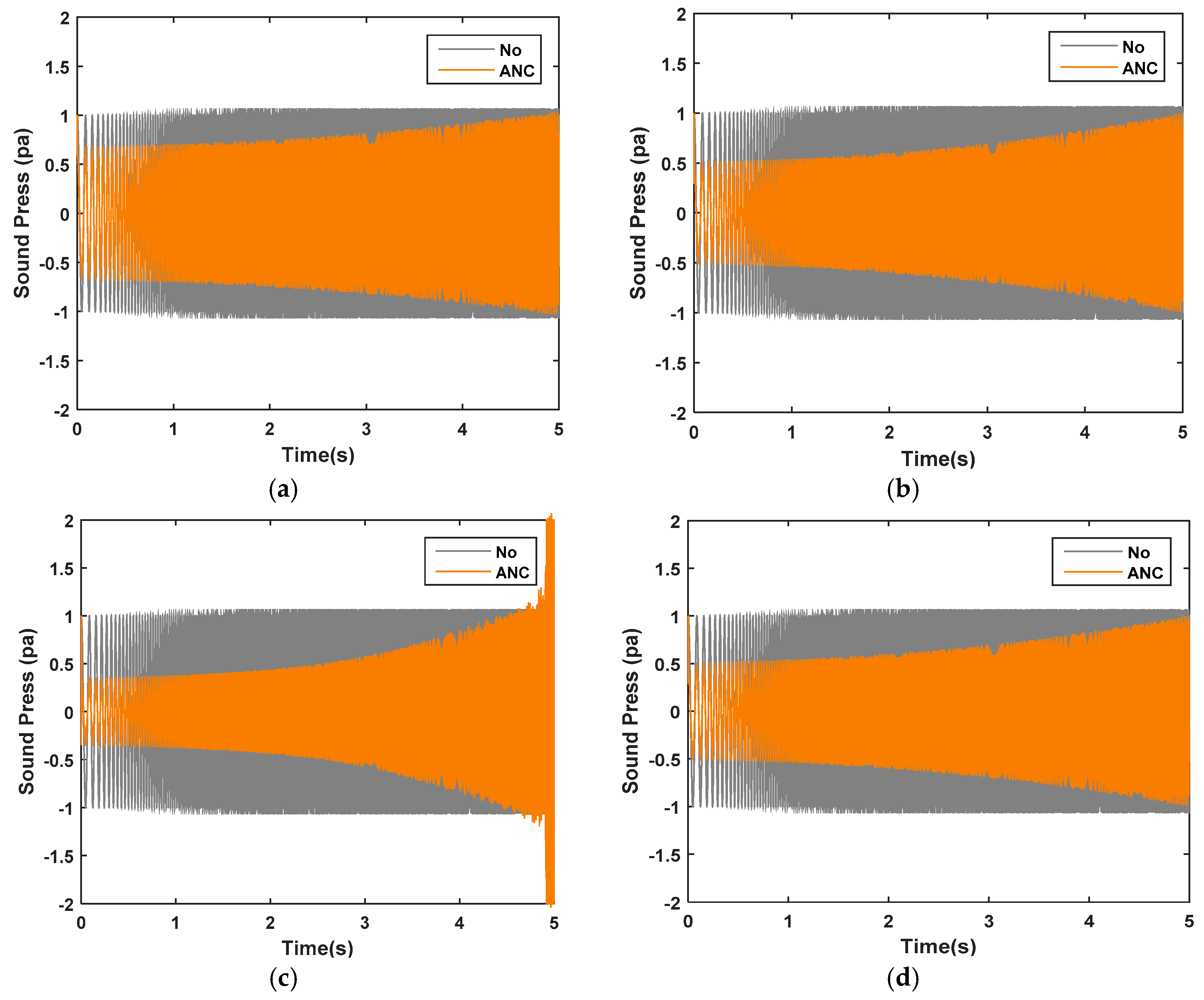
Figure 3 illustrates the time history of error signals controlled by the NLMS algorithm-based adaptive notch filter with two weights (L = 2). Different step sizes are used to observe the resulting effect of convergence. In Figure 3, the letter “u” denotes step size. Figure 3a–c illustrate the time history of errors controlled by the NLMS-algorithm-based adaptive notch filter with different step sizes of = 0.5, = 2, and = 3, respectively, but the leakage factor is 0.5. Figure 3d shows the comparison of power spectrum density (PSD). From these results, it can be observed that the convergence of the error signal is fast initially as the step size increases, but that the amplitude of the error signal diverges eventually. The adaptive notch filter cannot trace and control the time-varying signal with fast frequency change. Because the frequency bandwidth of the notch filter is very narrow it is not suitable when the frequency of the signal to be controlled is changed. Therefore, it is finally diverged. Subsequently, in order to observe the effect of leakage, different leakage factors are applied to the leaky NLMS algorithm in Equation (11) with the same step size ( = 2).
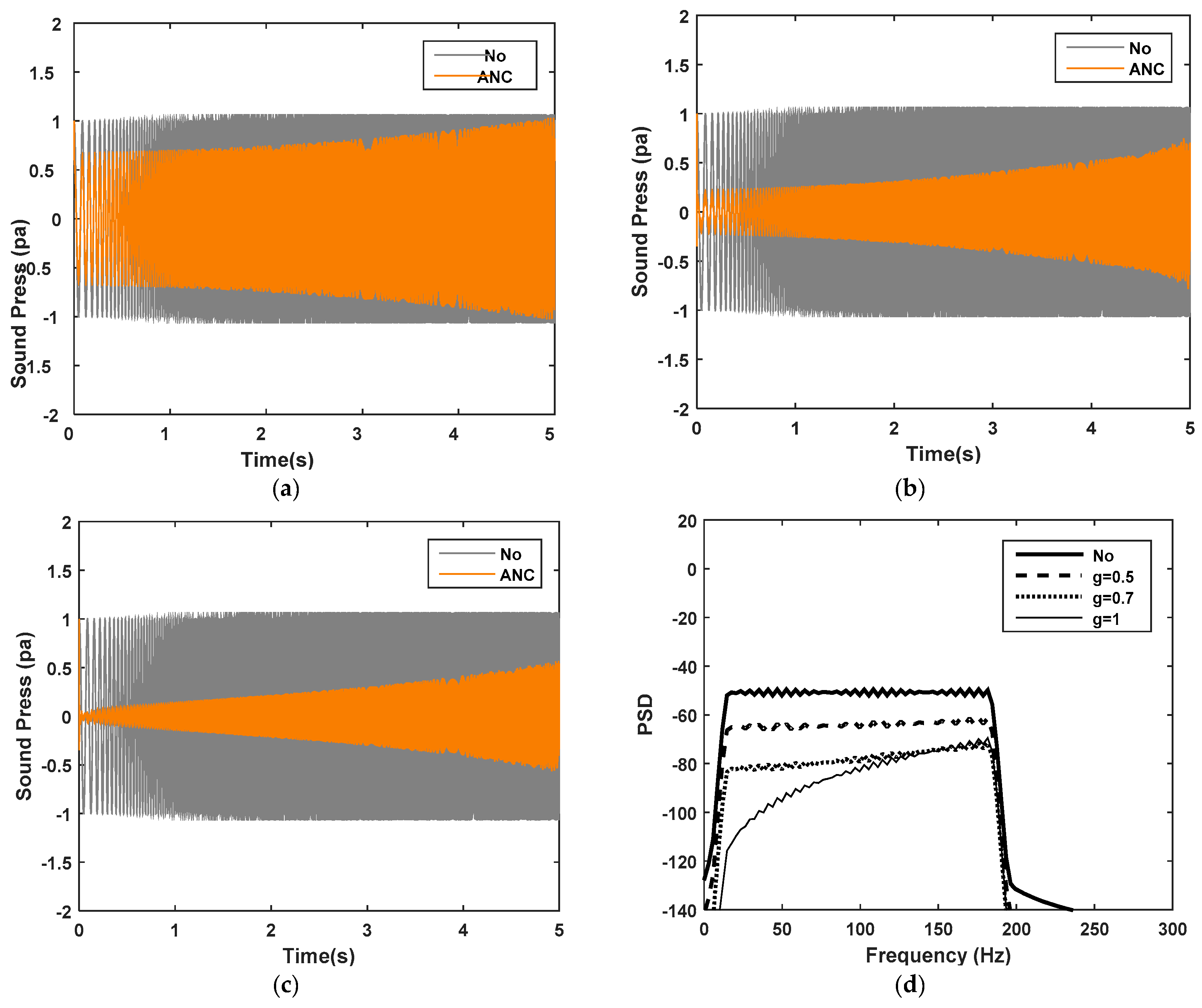
Figure 4a–c illustrates the time history of the error signal controlled by the NLMS-algorithm-based adaptive notch filter with different leakage factors of γ = 0.5, γ = 0.7, and γ = 1.0, respectively, and the step size is 0.5. In Figure 4, the letter “g” denotes leakage factor. According to these results, the amplitude of the error signal diverges eventually. Even with the selection of any leakage factor, the controller cannot work stably. Subsequently, in order to observe the effect of frequency variation, reference signals with five different sweep rates are used.
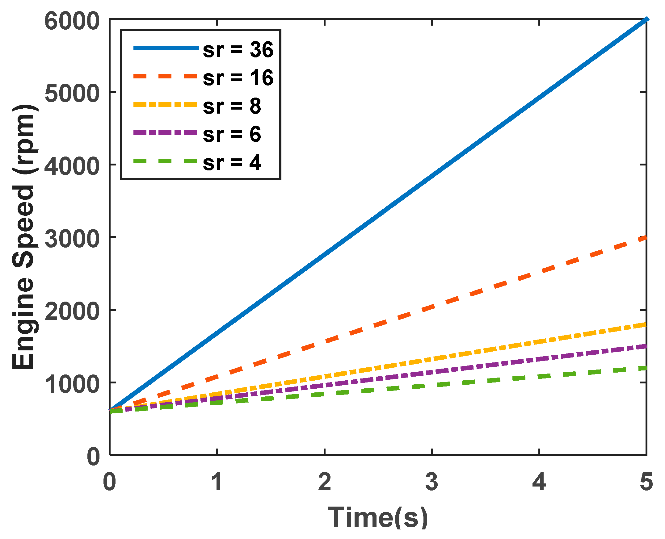
Figure 5 shows the variation of instantaneous frequency (fi = rpm/60) of the five references. The sweep time is 5 s for all the references. The selected sweep rates, which are calculated using ∆fi/∆time, are 4, 6, 8, 16, and 36 s.
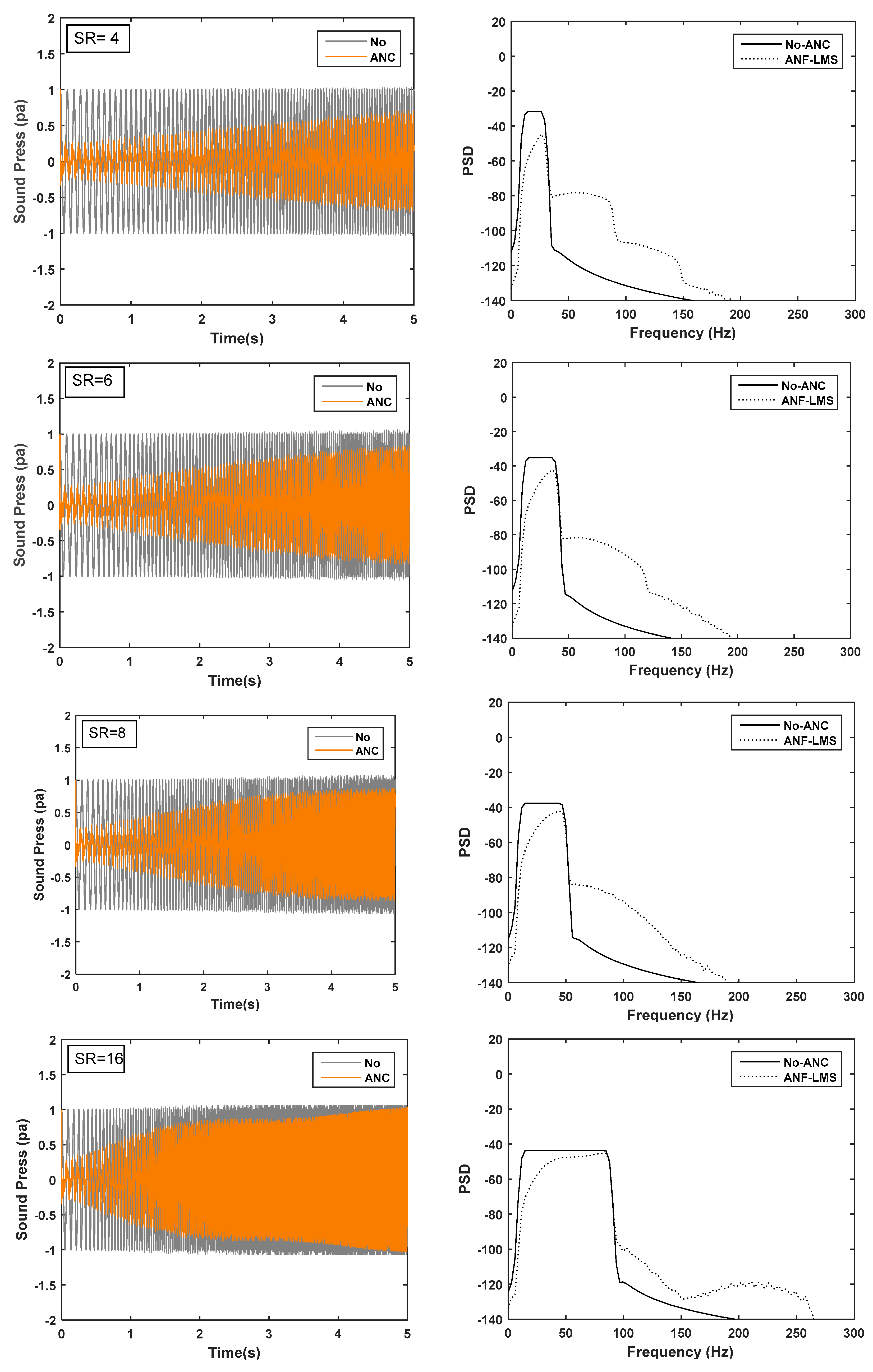
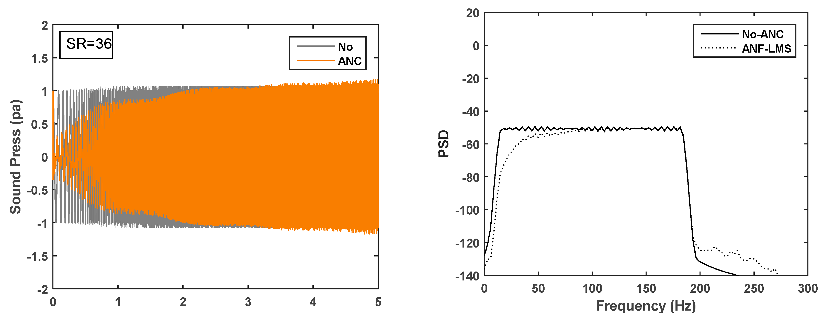
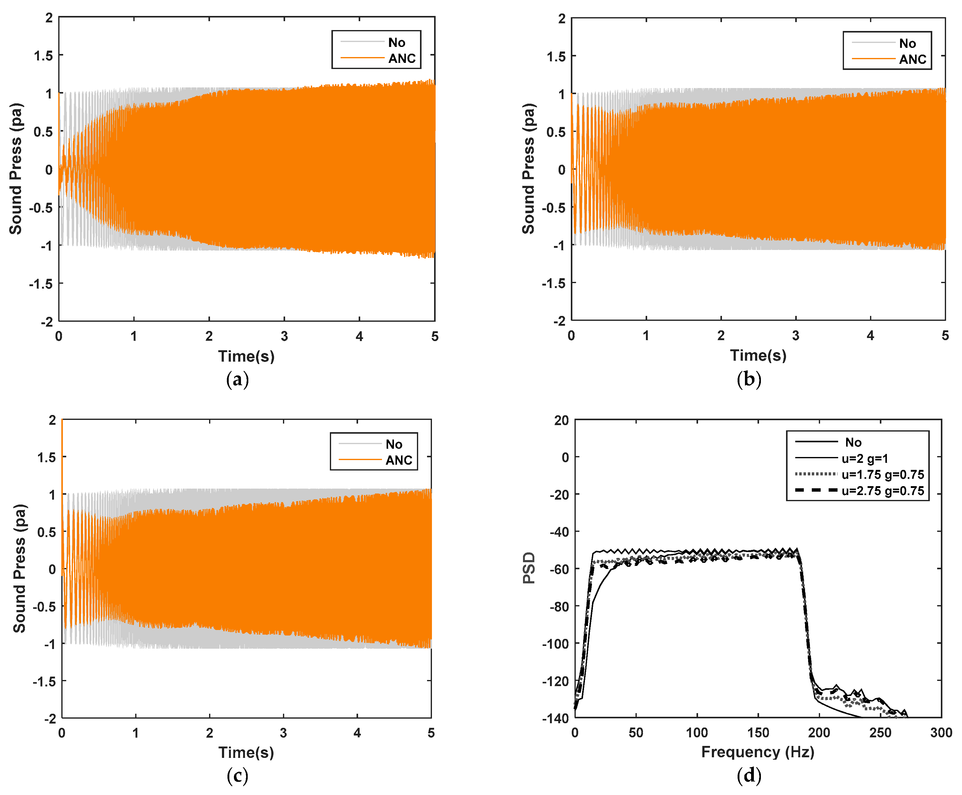
Figure 6 illustrates the time history and PSDs of the error signals controlled by the leaky NLMS algorithm-based adaptive notch filter with two weights (L = 2), leakage factor (γ = 1), and step size = 2. These results demonstrate that the error signals do not converge and are not stable for all the cases with different sweep rates. Finally, we attempted to determine the optimal step size and leakage factor for signal 1. Using the previous simulation results, we first used the step size of = 2 and leakage factor of γ = 1 in this simulation.
The time history of the error signal is shown in Figure 7a. The error signal still diverges. In order to converge the error signal, we decreased the step size from = 2 to = 1.75 and the leakage factor from γ = 1 to γ = 0.75 corresponding to the rule of leaky LMS algorithm. The error signal converges initially as shown in Figure 7b but eventually it diverges. For faster convergence at the start, we increased the step size from = 2 to = 2.75. In this case, a jump in the error signal appears initially as shown in Figure 7c and eventually the error diverges. In any of the cases, the PSD of the error signal is not attenuated as shown in Figure 7d. It can be concluded that the leaky NLMS-algorithm-based adaptive notch filter is not suitable for active cancellation of the rapid frequency varying disturbances.
Figure 8a shows a comparison between the time history of error signals controlled by the LMS-algorithm-based adaptive notch filter and the OW-LMS algorithm. The error signal controlled by the adaptive notch filter shows incomplete convergence as the frequency increases according to the time increment. However, the OW-LMS algorithm with a short length (L = 30) of weight vectors is sufficient to attenuate this frequency modulated signal. The results show fast and stable convergence. The PSD function of the error signals is compared, and the results are plotted as shown in Figure 8c. According to these results, the OW-LMS algorithm exhibits superior control performance compared to the conventional method for the frequency-modulated signal. Figure 8e shows an image map of the power spectrum of the weight vector of the adaptive filter used in the OW-LMS algorithm. This map shows the adaptive performance of the filter. Since the length of the weight vector is 30, the frequency bandwidth of the filter is 200 Hz as shown in Figure 8g. In the case of signal 1, according to Equation (15), the optimal length (L) of the weight vector is changed from 300 (at 600 rpm) to 60 (at 6000 rpm) because ∆k is 1 (single frequency) and fs is 3000 Hz. If we use the adaptive filter with the largest optimal length (L = 300) of weight vector, the convergence is faster and more stable as compared to other algorithms as shown in Figure 8b. The attenuation level of the error signal is the largest in Figure 8d. The frequency bandwidth of the adaptive filter is narrow as shown in Figure 8f,h.
In conclusion, in the case of a sinusoidal signal with single frequency modulation (i.e., single order signal), the OW-LMS algorithm with the optimal length of weight vector can be used for sufficient control of the error signal. Its convergence performance is better than that of the conventional algorithm.
Signal 2. Frequency-modulated signal (multi-order signal)
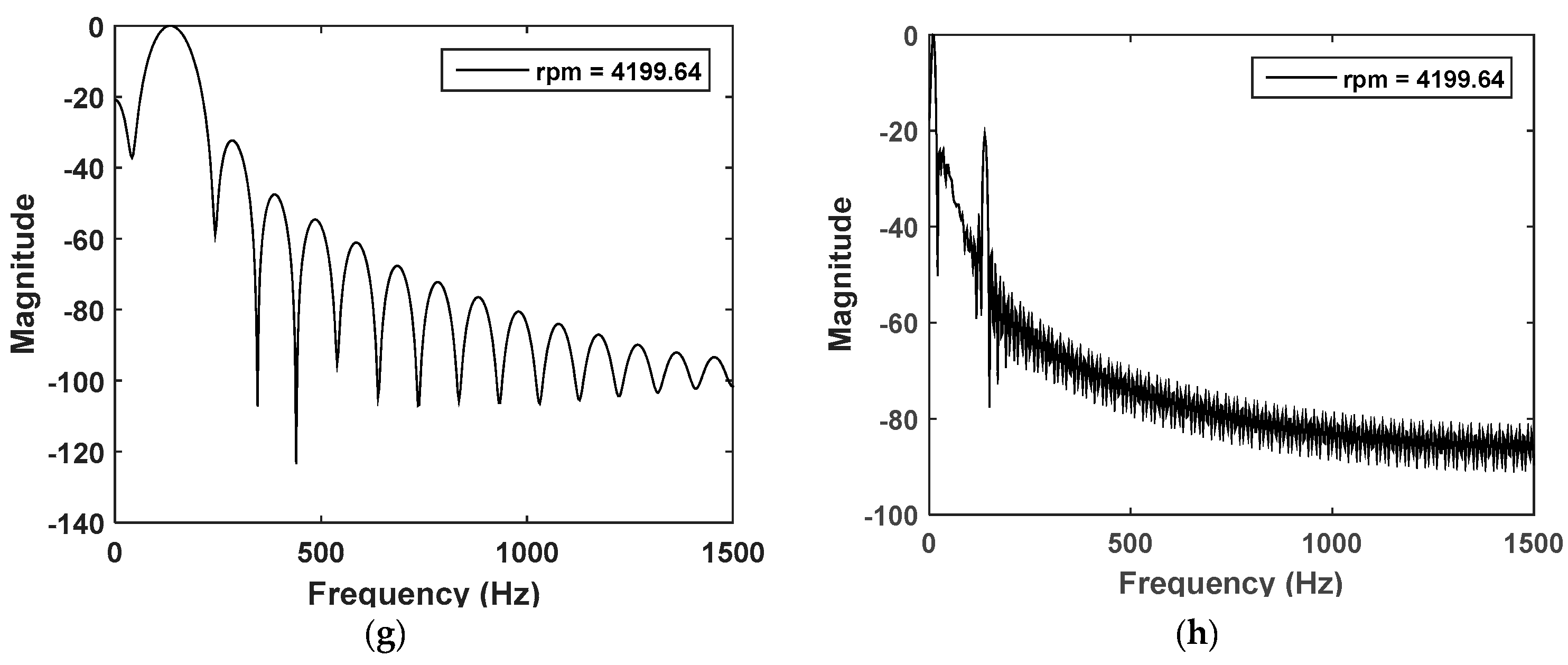
A frequency-modulated signal with three orders is applied to the two ANC systems again. Figure 9a illustrates the time history of signal 2 controlled by the conventional method. The controller cannot sufficiently reduce the order signals without divergence. Figure 9b illustrates the time history of signal 2 controlled by the OW-LMS algorithm. Two weight vectors were used in the controller. The controller with a long weight vector (L = 300) converged after 1 s, whereas the controller with a short weight vector (L = 30) converged after 2 s. From Equation (15), the optimal filter length is 18,000/RPM since ∆k is 2 and the sampling frequency is 3000 Hz. Therefore, the length of the weight vector should be 300 since the minimum rotational speed is 600 rpm (10 Hz) for this signal. As the rotational speed increases, the length of weight vector can be decreased for stable control. In this simulation, the controller with a long weight vector (L = 300) converged at low rotational speed, but the controller with a short weight vector (L = 30) converged at high rotational speed. Figure 9c,d show the short-time Fourier transform (STFT) for the signals controlled by the OW-LMS algorithm. Expectedly, at a low rotational speed of less than 1 s, the controller with a short weight vector still converges as shown in Figure 9c, whereas the controller with a long weight vector has converged, as shown in Figure 9d. Figure 9e shows the STFT for the error signal controlled by the conventional algorithm. The order error signal was not completely attenuated by the controller with the conventional algorithm. Figure 9f shows a comparison of PSD functions of error signals obtained by the three controllers. From these results, we determined that the OW-LMS algorithm is superior for the active control of a frequency modulated signal compared to the conventional method.
4. OW-FxLMS Algorithm for ANC of Engine Noise
The active noise canceller of the OW-FxLMS algorithm can be used to eliminate intense sinusoidal sounds with frequency modulation. This method is applied to engine noise cancellation inside a vehicle because the engine noise is dominant. The engine noise is comprised of multiple intense sinusoidal signals. This signal is synchronized with the rotating speed of the engine and is a frequency-modulated signal. Other noise sources such as wind noise, tire noise, and high noise environments interfere with the engine noise [1].
Figure 10 illustrates an active noise canceller for the engine noise of a vehicle. The canceller employs controller area network (CAN) bus data or a directional sensor to measure the instantaneous frequency fi corresponding to the rotating frequency of the engine, and four microphones to measure the interior noise containing engine noise and other noise. The measured instantaneous frequency is used for the generation of the reference signal. A recursive discrete-time oscillator is used to generate the reference signal [23]. The reference signal is processed by the adaptive filter to equalize it with the engine noise component of the primary noise contaminated by the other noise signals. It is subsequently subtracted to cancel out the engine noise component in the primary noise.
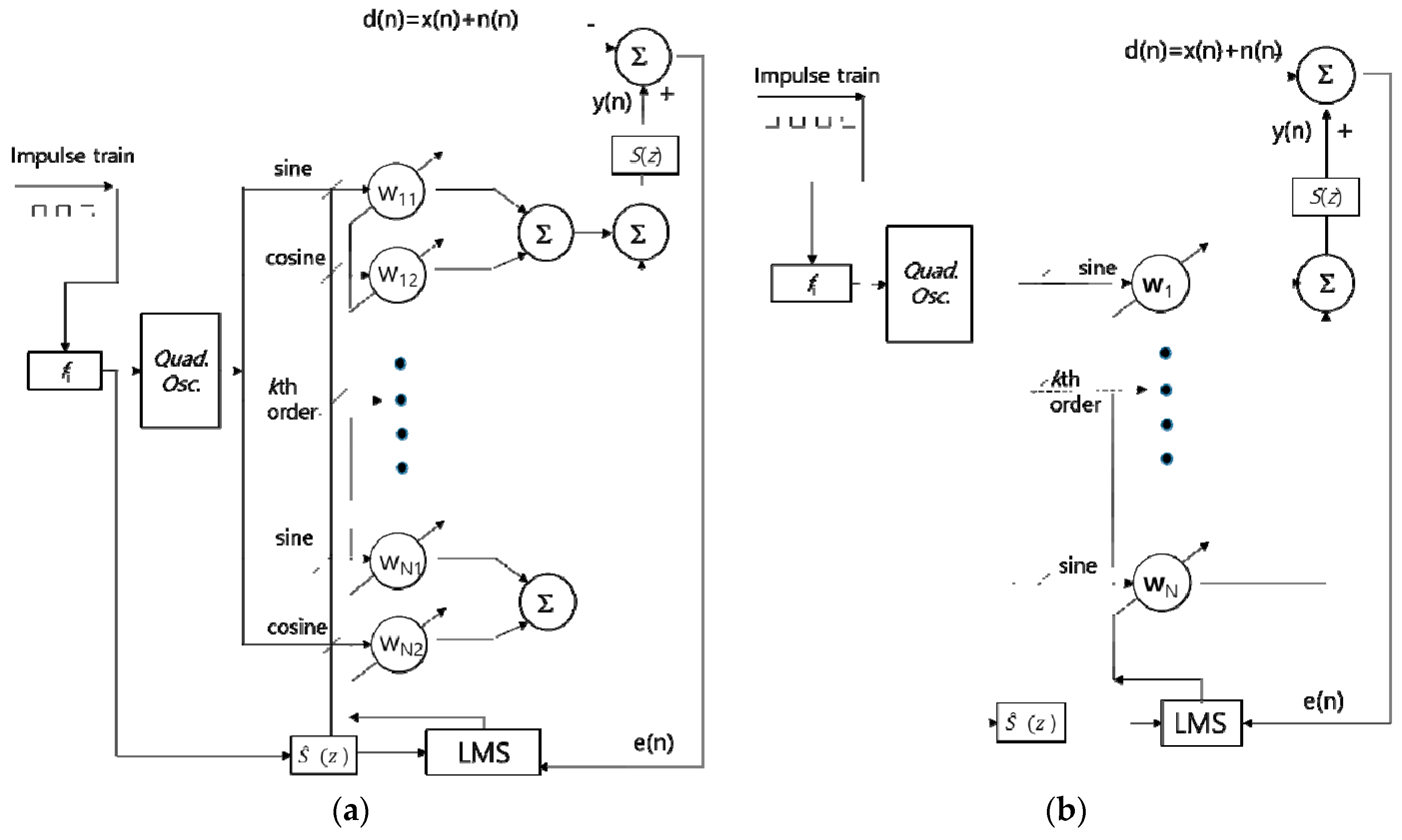
Figure 11 shows the block diagram of the FxLMS-algorithm-based adaptive notch filter and the OW- FxLMS algorithm for the application of ANC to engine noise inside a vehicle. In the FxLMS -algorithm-based adaptive notch filter, two adaptive weights, wi1 (n) and wi2 (n), were used for each order. In the OW- FxLMS algorithm, the adaptive weight vector w(n) with different filter lengths was used for each order. The length of each weight vector was related to the total delay of the ANC system. The secondary path was considered for the application of ANC to engine noise.
5. Application of the OW-Fxlms Algorithm to ANC of Interior Noise
5.1. Experimental Setup and Procedure
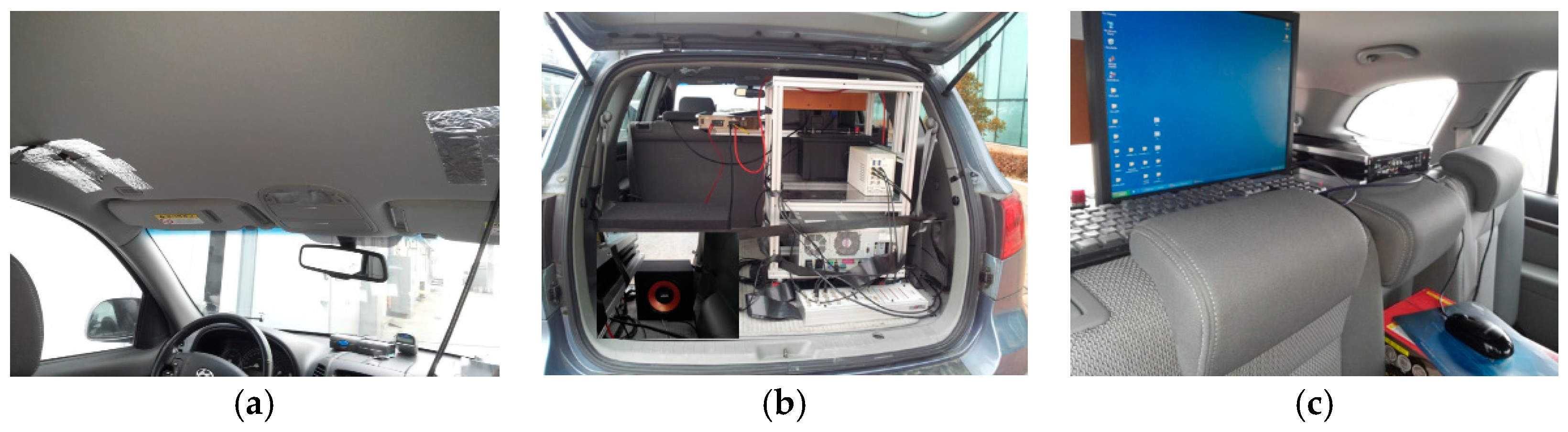
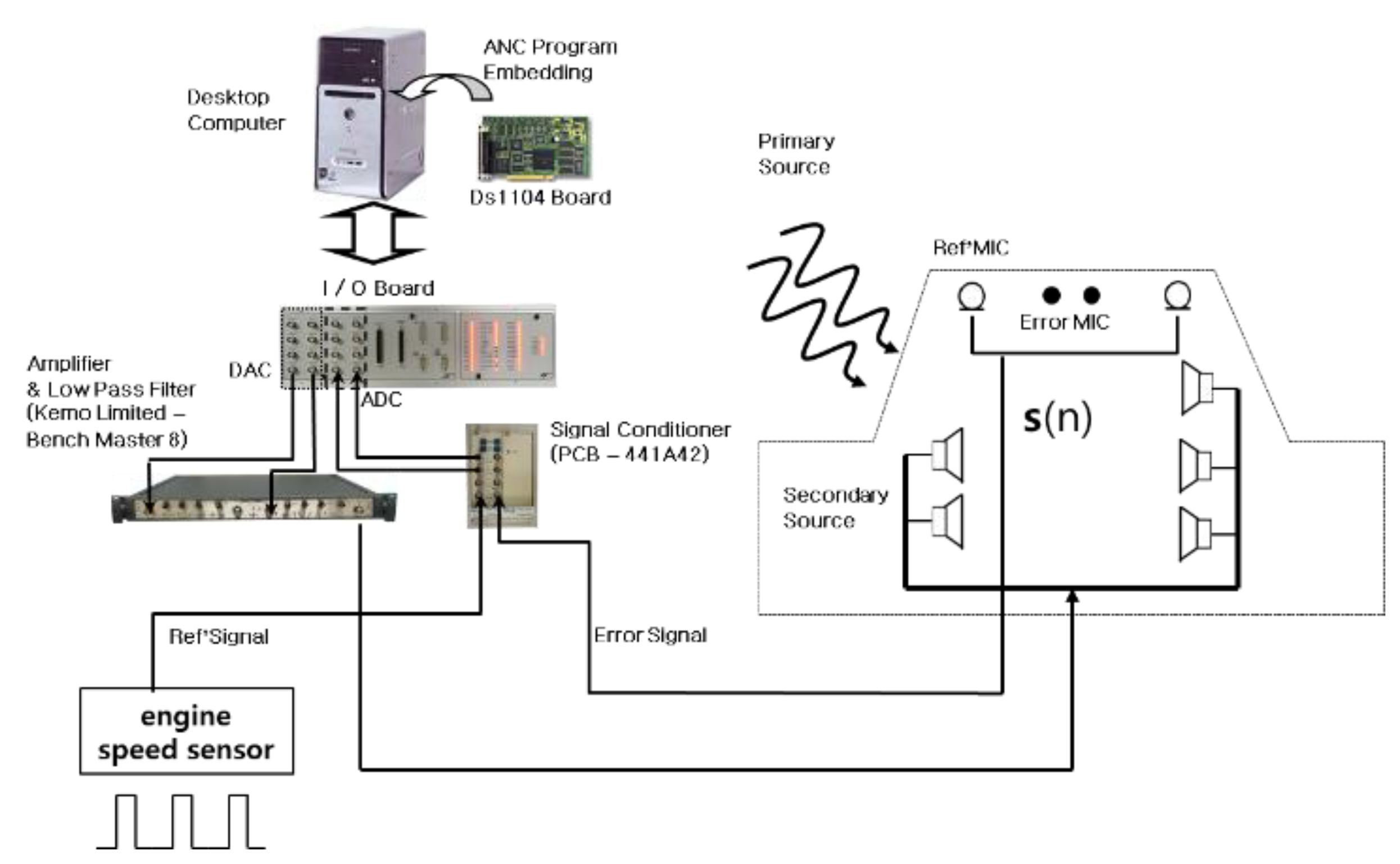
A sport utility vehicle was used for the application of ANC to interior noise. The test car is SNATAFE made by Hyundai motor company as shown in Figure 12. A 2.2 L diesel engine was used in the powertrain of this vehicle. The instruments used for the ANC were loaded inside the vehicle. The equipment used in the ANC system is shown in Figure 13.
Four microphones were used for the measurement of error signals, and were attached to the roof of the vehicle. Five speakers were used as the secondary sound sources required to cancel the primary noise sources inside the vehicle [26]. The error signals were transferred to the input channels of a DSP control board (Ds 1104, dSPACE, Paderborn, Germany) via a signal conditioner (441-A42, PCB Company, Depew, NY, USA). The software used to implement the adaptive algorithm is MATLAB (Simulink, MathWorks, Natick, MA, USA). The pulse signal, including the speed data of the engine, was detected by a camshaft position sensor and transferred to the input channels of the dSPACE control board. Both input data streams were transferred to the control computer via an analog-to-digital (A/D) converter in the dSPACE control board. The pulse signal was used for the calculation of the instantaneous frequency and reference signal. The reference signal was convolved by the estimated impulse response of the secondary path. The signal was the input x’(n) of the LMS algorithm. The adaptive filter w(n) was updated by using error data e(n) and input data x’(n).
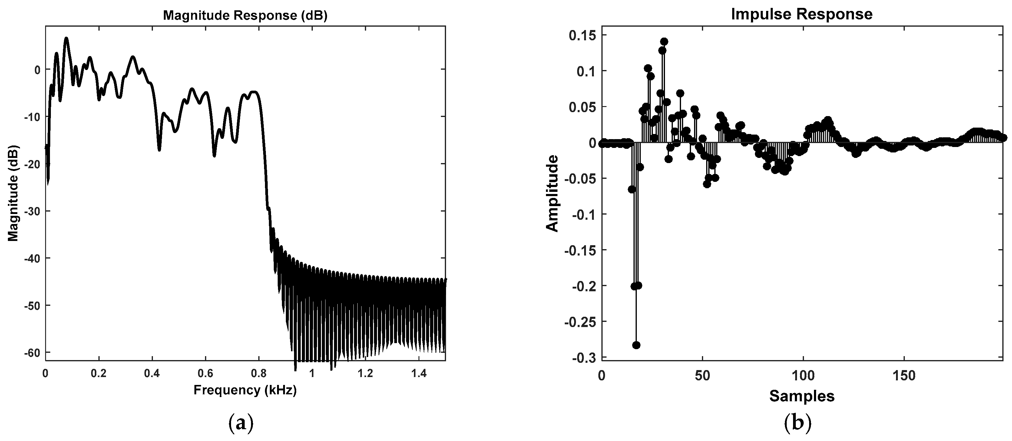
5.2. Measurement of the Impulse Response of the Secondary Path
The impulse response of the secondary path was estimated by using the LMS algorithm. A block diagram for the estimation of the impulse response in the secondary path is given in [26]. A random white signal was used as the input data because we assume that the secondary path is a linear system. The impulse response of the secondary path was obtained after sufficient convergence. The transfer function S(z) of the secondary path was obtained by performing the z-transform for the impulse response. The results are plotted in Figure 14.
5.3. Application of Adaptive Algorithms to ANC for Interior Noise
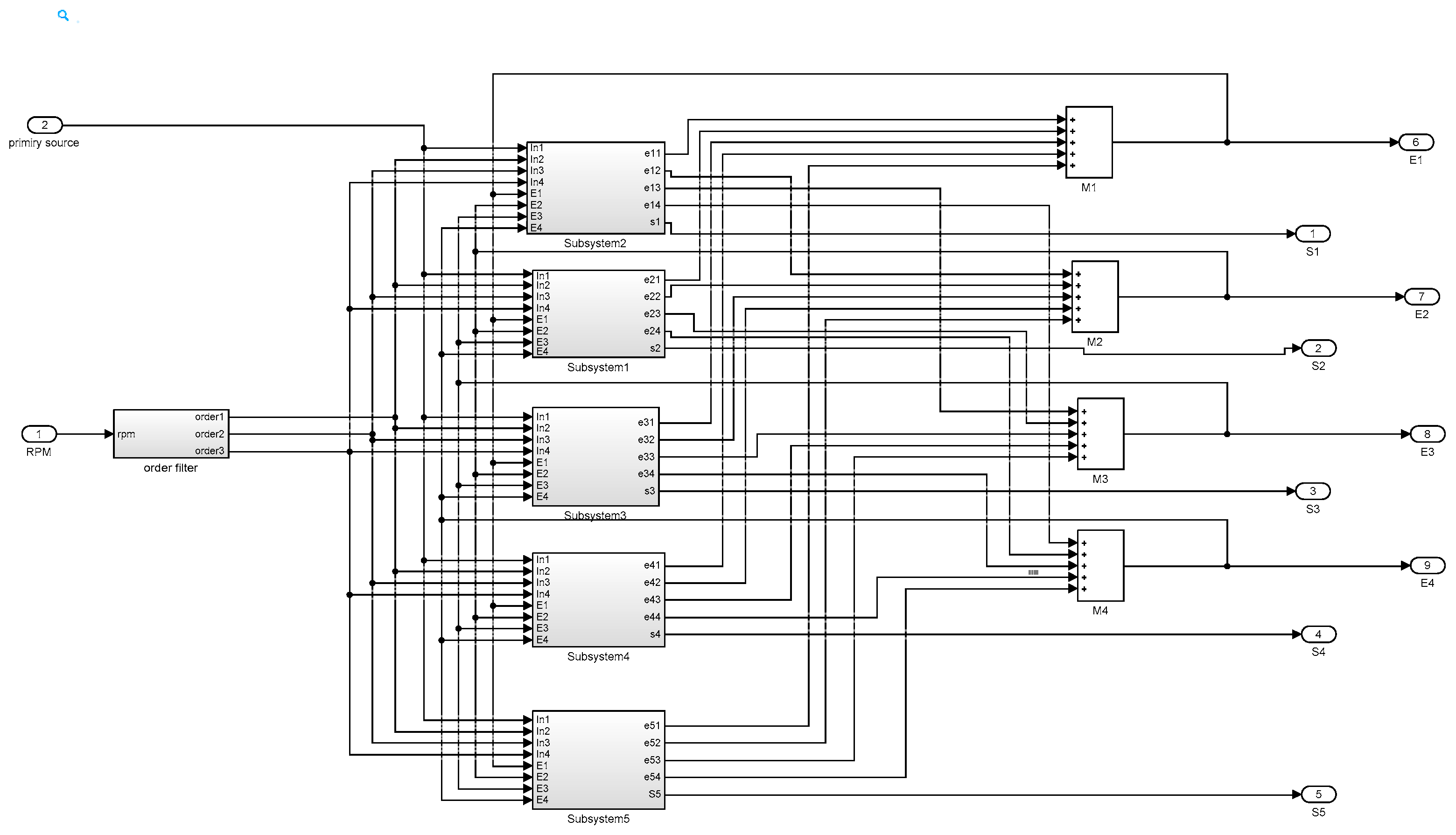
In order to drive the vehicle with the ANC system on the road, five speakers, a control computer, monitor, and the dSPACE control board were placed in the test vehicle, and the microphones were attached to the roof of the test vehicle. In this case, a multichannel ANC system was used. The algorithm is the expansion of a channel ANC. The Simulink based block diagram used for this test is plotted as shown in Figure 15. There are 5 subsystems which include adaptive order filter and OW-FXLMS algorithm to control the interior noise measured by 4 microphone and 5 secondary speakers. S1, S2, S3, S4 and S5 means the secondary speaker and M1, M2, M3 and M4 means the microphone attached in the car. The primary source which was recorded inside of test car and supplied to the multi-channel ANC system. In each subsystem, the OW-FXLMS algorithms update the adaptive filter using the error signals (E1, E2, E3, E4) measured from 4 microphones and primary source signal. For example, the output of subsystem 1 is the sound signal for speaker S1 sound and error signals (e1j) which is related to each j-th reference order signal. The sum of error signals (e1j) is the error signal of M1. In the real time process, primary source is not necessary and the signals from error microphones become noise source signal.
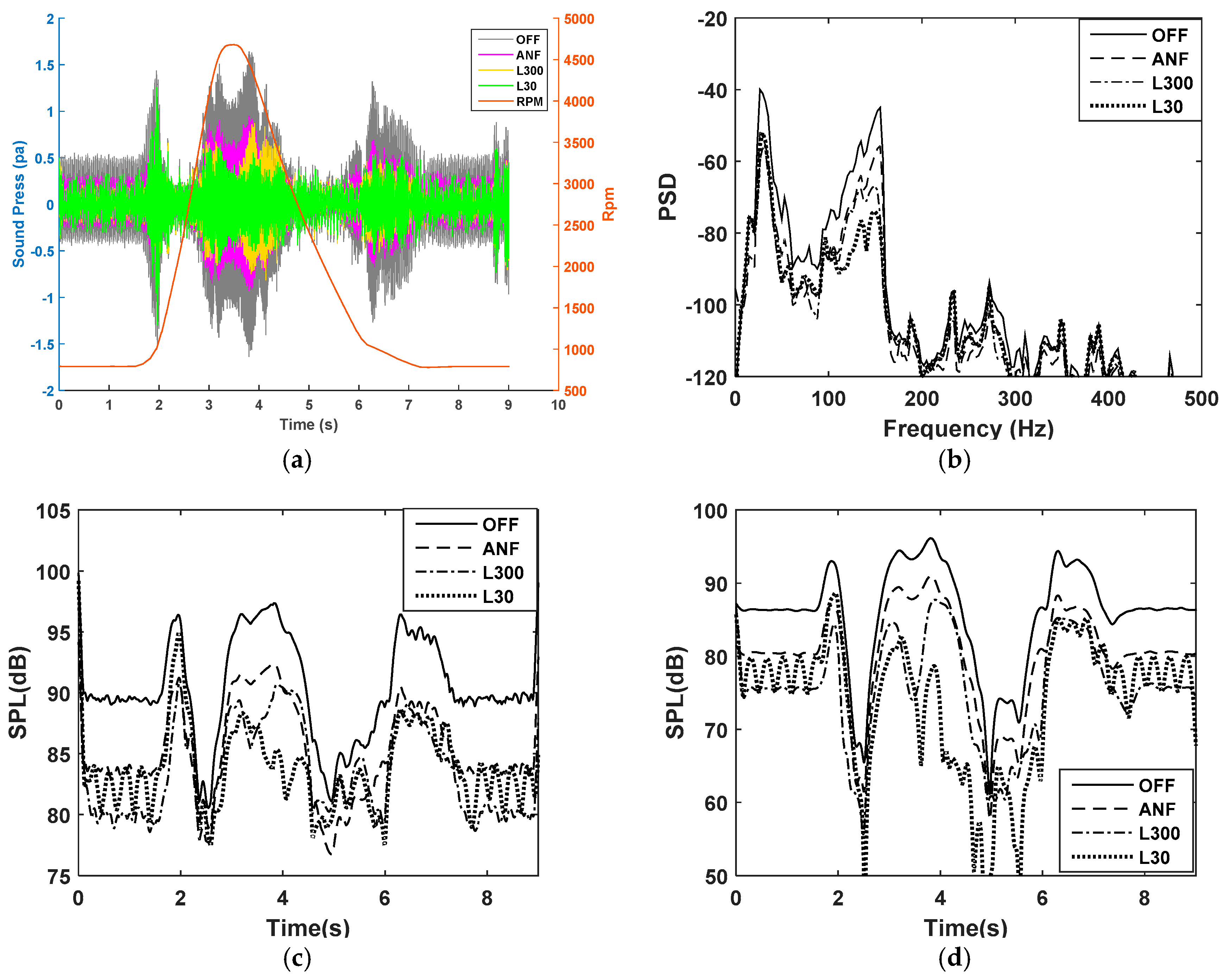
When the engine speed increased under a no-load condition, the ANC system was operated and the sound pressure of the interior noise was measured by error microphones. The engine speed was increased from 1000 rpm to 4500 rpm. The engine was under the no-load condition for this test, and the engine speed was increased rapidly from 800 rpm at idle to 4500 rpm during the course of 2 s. Figure 16a illustrates a comparison of the time history of the interior noise at the driver seat, which was controlled by two active control systems. Figure 16b illustrates the spectrum analysis of the interior noise signal. The PSD of the interior noise signal was reduced to 30 dB above 80 Hz. Figure 16c,d illustrate the results of order analysis of the interior noise. At 1200 rpm, there is a booming noise, and the other wide booming noise occurred from 3000 to 4500 rpm. These booming noises were attenuated by the controllers. The controller with the OW- FxLMS algorithm with a short filter length (L = 30) demonstrated the best performance among the three algorithms. Since the optimal length of weight vector is 18,000/RPM, a short filter length (L = 30) is sufficient for the control of these booming noises. This algorithm achieved a significant reduction in the interior noise around 4500 rpm, which is the second-order boom noise as shown in Figure 16c,d. The sound pressure level (SPL) of the interior noise was reduced to 25 dB.
This booming noise corresponds to the resonance of the second path, as shown in Figure 14. The OW-FxLMS algorithm with a long length (L = 300) and the FxLMS-algorithm-based adaptive notch filter reduced the booming noise, but not sufficiently, since the frequency bandwidth of the adaptive filters used for these algorithms is too narrow to reduce wideband noise, and the speed is changed too quickly (within 2 s). The disadvantage of the OW- FxLMS algorithm with a long length (L = 30) is the generation of a beating sound at idle speed owing to its wide bandwidth. However, the sound pressure of the beat noise was too low to be heard.
5.4. Performance of the ANC System with OW-FxLMS
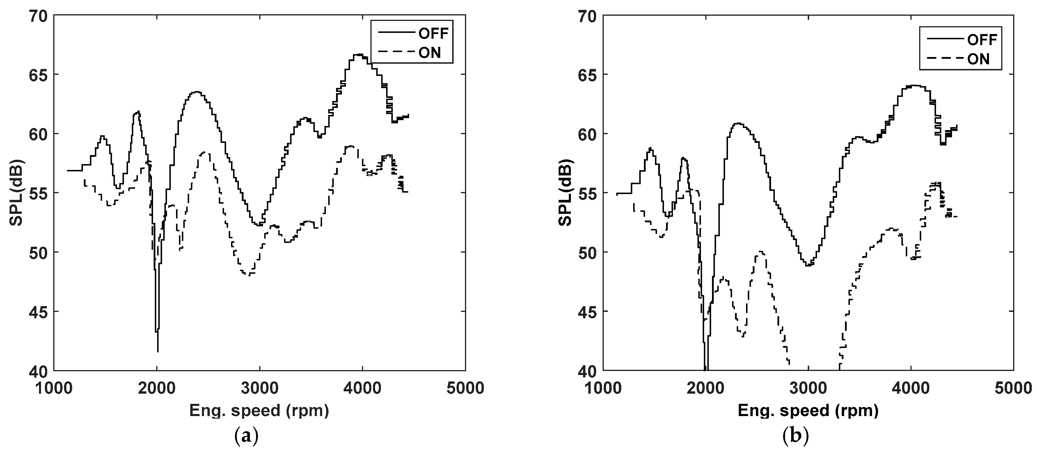
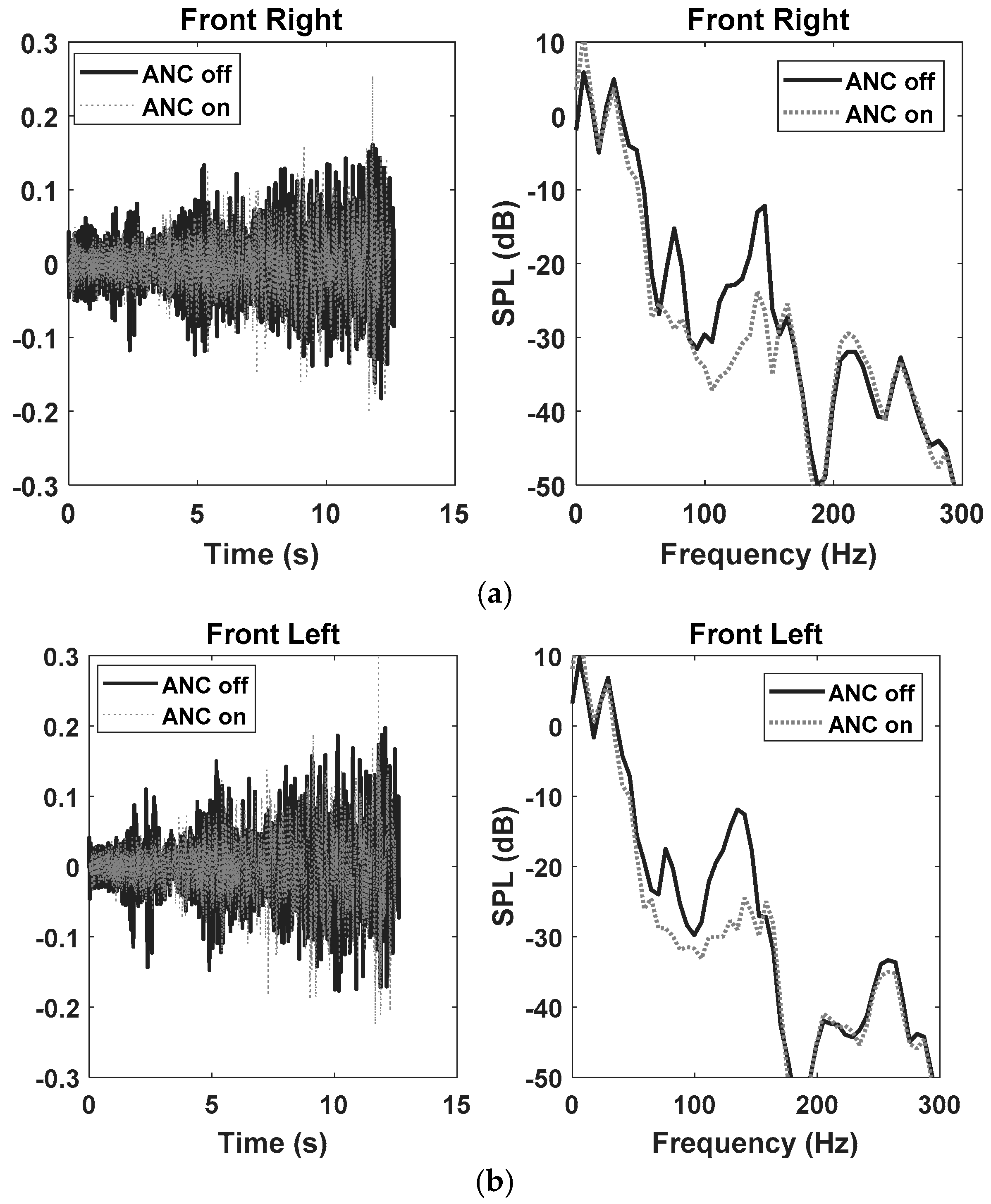
Figure 17 shows the sound pressure of the interior noise in the test vehicle while driving on the road. The upper solid line is the SPL of the interior noise, and the lower dotted line is the actively controlled SPL. Figure 17a shows the overall sound pressure, and Figure 17b shows the sound pressure of the second-order component of the engine rotating frequency. The second order is generally related to the booming noise. The engine was under full load for this test while driving the car on the road and the engine speed increased rapidly from 1000 to 4500 rpm during the course of 10 s. In this case, the higher orders were not controlled because the calculation speed of the ANC system was beyond the capacity of dSPACE, and the noise of the second order was dominant. From these results, we suggest that the new ANC system using the OW-FxLMS algorithm performed well in reducing the sound pressure of the interior noise related to the harmonic components of engine rotating speed. Figure 18 shows the performance of the ANC system with the new algorithm for full load condition of the engine. Figure 18a,b the results of active noise cancellation at left seat (driver seat) and at right seat (passenger seat) respectively.
6. Conclusions
We present a new algorithm to control the engine noise in the cabin of a car. The proposed algorithm is called the OW-FxLMS algorithm, which uses an adaptive filter with an optimal filter length. The optimal filter length is determined to have a frequency bandwidth less than the frequency bandwidth between the orders to be controlled by the controller. This algorithm is suitable for the reduction of engine noise associated with the rotating frequency of the engine. In the last thirty years, many algorithms have been developed for the control of engine noise. In this study, as a representation of the conventional methods, the performance of the FxLMS-algorithm-based adaptive notch filter was tested for comparison with the performance of the new algorithm. Three signals were synthesized for the simulation. According to our simulation results, both algorithms are suitable for the control of a sinusoidal signal with constant frequency. However, the OW-FxLMS algorithm is superior to the conventional algorithm for the control of amplitude- and frequency-modulated sinusoidal signals, such as the engine noise with fast frequency change when the car is accelerated for a short time. The algorithm was applied to the control of booming noise in a sport utility car to test the practical implementation of the proposed algorithm. The SPL of the interior noise of this test car was actively controlled by this algorithm, and was attenuated to 25 dB under a no-load condition, whereas the reduction of the sound pressure was attenuated to 2–3 dB by the conventional algorithm. Finally, the ANC system with the proposed algorithm was used to control the interior noise while driving on the road. Under full engine load, the SPL of the interior noise in the test vehicle was significantly reduced. The performance of the new ANC system is therefore, excellent for the attenuation of engine noise in the cabin of a car.
Author Contributions
S.-K.L. contributed to simulation and algorithm development and writing the paper. S.L. contributed to Simulink programming. T.S. contribution to the vehicle experimental test.
Funding
This work was supported by Mid-career Researcher Program through NRF of Korea grant funded by the MEST (No. 2016R1A2B2006669).
Acknowledgments
This work was supported by Inha University.
Conflicts of Interest
This work was supported by Inha University.
References
- Kim, T.G.; Lee, S.K.; Lee, H.H. Characterization and quantification of luxury sound quality in premium-class passenger cars. Proc. Inst. Mech. Eng. Part D J. Autom. Eng. 2009, 223, 343–353. [Google Scholar] [CrossRef]
- Lee, H.H.; Lee, S.K. Objective evaluation of interior noise booming in a passenger car based on sound metrics and artificial neural networks. Appl. Ergon. 2009, 40, 860–869. [Google Scholar] [CrossRef] [PubMed]
- Lee, S.K. Objective Evaluation of Interior Sound Quality in Passenger Cars during Acceleration. J. Sound Vib. 2008, 310, 149–168. [Google Scholar] [CrossRef]
- Elliott, S.J. A Review of Active Noise and Vibration Control in Road Vehicles; Technical Memorandum, No. 981; ISVR, University of Southampton: Southampton, UK, 2008. [Google Scholar]
- Samarasinghe, P.N.; Zhang, W.; Abhayapala, T.D. Recent Advances in Active Noise Control inside Automobile Cabins: Toward quieter cars. IEEE Signal Process. Mag. 2016, 33, 61–73. [Google Scholar] [CrossRef]
- Elliott, S.J. Signal Processing for Active Control; Academic Press: New York, NY, USA, 2001. [Google Scholar]
- Kuo, S.M.; Morgan, D.R. Active Noise Control Systems Algorithms and DSP Implementations; John Wiley & Sons: New York, NY, USA, 1996. [Google Scholar]
- Lee, S.K. Adaptive Signal Processing and Higher Order Time Frequency Analysis for Acoustic and Vibration Signatures in Condition Monitoring. Ph.D. Thesis, ISVR, University of Southampton, Southampton, UK, 1998. [Google Scholar]
- Hykin, S. Adaptive Filter Theory, 5th ed.; Pearson: Boston, MA, USA, 2014. [Google Scholar]
- Pritzker, Z.; Feuer, A. Variable length stochastic gradient algorithm. IEEE Trans. Signal Process. 1991, 997, 1001. [Google Scholar] [CrossRef]
- Bilcu, R.C.; Kuosmanen, P.; Egiazarian, K. A new variable length LMS algorithm: Theoretical analysis and implementations. In Proceedings of the 9th International Conference on Electronics, Circuits and Systems, Dubrovnik, Croatia, 15–18 September 2002. [Google Scholar]
- Nascimento, V.H. Improving the initial convergence of adaptive filters: Variable-length LMS algorithms. In Proceedings of the 14th International Conference on Digital Signal Processing, DSP 2002, Santorini, Greece, 1–3 July 2002. [Google Scholar]
- Li, C.Y.; Chu, S.I.; Tsai, S.H. Improved Variable Step-Size Partial Update LMS Algorithm Green Technology and Sustainable Development (GTSD). In Proceedings of the International Conference on Green Technology and Sustainable Development, Kaohsiung, Taiwan, 24–25 November 2016. [Google Scholar]
- Widrow, B. Adaptive Signal Processing, 1st ed.; Prentice Hall: Upper Saddle River, NJ, USA, 1985. [Google Scholar]
- Kim, E.Y.; Kim, B.H.; Lee, S.K. Active Noise Control in a Duct System Based on a Frequency-estimation Algorithm and The FX-LMS Algorithm. Int. J. Autom. Technol. 2013, 14, 291–299. [Google Scholar] [CrossRef]
- Sun, X.; Liu, N.; Meng, G. Adaptive frequency tuner for active narrowband noise control systems. Mech. Syst. Signal Process. 2009, 23, 845–854. [Google Scholar] [CrossRef]
- Bismor, D.; Czyz, K.; Ogonowski, Z. Review and Comparison of Variable Step-Size LMS Algorithms. Int. J. Acoust. Vib. 2016, 21, 24–39. [Google Scholar]
- Oliveira, P.R.L.; Stallaert, B.; Janssens, K.; Auweraer, H.V. NEX-LMS: A novel adaptive control scheme for harmonic sound quality control. Mech. Syst. Signal Process. 2010, 24, 1727–1738. [Google Scholar] [CrossRef]
- Kim, H.W.; Park, H.S.; Lee, S.K.; Shin, K. Modified-Filtered-u LMS Algorithm for Active Noise Control and Its Application to a Short Acoustic Duct. Mech. Syst. Signal Process. 2011, 25, 475–484. [Google Scholar] [CrossRef]
- Lee, S.K.; Lee, S.M.; Kang, I.D.; Shin, T. Active Sound Design for a Passenger Car Based on Adaptive Order Filter. In Proceedings of the Internoise 2014, Melbourne, Australia, 16–19 November 2014. [Google Scholar]
- Lee, S.M.; Lee, S.K.; Park, D.C.; Kim, S. A Novel Method for Objective Evaluation of Interior Sound in a Passenger Car and Its Application to the Design of Interior Sound in a Luxury Passenger Car. In Proceedings of the NoiseCon 2017, Grand Rapids, MI, USA, 12–14 June 2017. [Google Scholar]
- Kraus, R.; Millitzer, J.; Hansmann, J.; Wolter, S.; Jackel, M. Experimental study on active noise and active vibration control for a passenger car using novel piezoelectric engine mounts and electrodynamic inertial mass actuators. In Proceedings of the 25th International Conference on Adaptive Structure and Technologies (ICAST2014), Hague, The Netherlands, 6–8 October 2014. [Google Scholar]
- Bismor, D.; Pawelczyk, M. Stability Conditions for the Leaky LMS Algorithm Based on Control Theory Analysis. Arch. Acoust. 2016, 41, 731–739. [Google Scholar] [CrossRef] [Green Version]
- Turner, C.L. Recursive Discrete-time Sinusoidal Oscillators. IEEE Signal Process. Mag. 2003, 20, 103–111. [Google Scholar] [CrossRef]
- Righam, E. Fast Fourier Transform and Its Applications; Prentice Hall: Upper Saddle River, NJ, USA, 1988. [Google Scholar]
- Kim, S.J.; Lee, S.K. Prediction of structure-borne noise caused by the powertrain on the basis of the hybrid transfer path. Proc. Inst. Mech. Eng. Part D J. Autom. Eng. 2009, 223, 485–502. [Google Scholar] [CrossRef]
- Boashash, B. Estimating and interpreting the instantaneous frequency of a signal—Part 1: Fundamentals. Proc. IEEE 1992, 80, 520–538. [Google Scholar] [CrossRef]
Figure 1.
Narrowband FxLMS algorithm based adaptive notch filter.

Figure 2.
OW-FxLMS control algorithm based adaptive filter with optimized weights (OW).

Figure 3.
Time history and PSD of signal 1 controlled by the normalized least mean squares filter (NLMS) algorithm-based adaptive notch filter with two weights (L = 2) and leakage factor (γ = 0.5). (a) Time history ( = 0.5); (b) Time history ( = 2); and (c) Time history ( = 3); and (d) PSD.
Figure 3.
Time history and PSD of signal 1 controlled by the normalized least mean squares filter (NLMS) algorithm-based adaptive notch filter with two weights (L = 2) and leakage factor (γ = 0.5). (a) Time history ( = 0.5); (b) Time history ( = 2); and (c) Time history ( = 3); and (d) PSD.

Figure 4.
Time history and PSD of signal 1 controlled by the NLMS algorithm-based adaptive notch filter with two weights (L = 2) and leakage factor (γ = 0.5). (a) Time history (γ = 0.5); (b) Time history (γ = 0.7); and (c) Time history (γ = 1); and (d) PSD.
Figure 4.
Time history and PSD of signal 1 controlled by the NLMS algorithm-based adaptive notch filter with two weights (L = 2) and leakage factor (γ = 0.5). (a) Time history (γ = 0.5); (b) Time history (γ = 0.7); and (c) Time history (γ = 1); and (d) PSD.

Figure 5.
Variation of instantaneous frequency (fi = rpm/60) of five references.

Figure 6.
Time history and PSD of the signal 1 with different sweep rate controlled by the Leaky NLMS algorithm-based adaptive notch filter with two weights (L = 2), leakage factor (γ = 1), and step size = 2.
Figure 6.
Time history and PSD of the signal 1 with different sweep rate controlled by the Leaky NLMS algorithm-based adaptive notch filter with two weights (L = 2), leakage factor (γ = 1), and step size = 2.


Figure 7.
Time history and PSD of signal 1 controlled by the NLMS algorithm-based adaptive notch filter with two weights (L = 2) (a) Time history ( = 2, γ = 1); (b) Time history ( = 1.75, γ = 0.75); and (c) Time history ( = 2.75, γ = 0.75) and (d) PSD.
Figure 7.
Time history and PSD of signal 1 controlled by the NLMS algorithm-based adaptive notch filter with two weights (L = 2) (a) Time history ( = 2, γ = 1); (b) Time history ( = 1.75, γ = 0.75); and (c) Time history ( = 2.75, γ = 0.75) and (d) PSD.

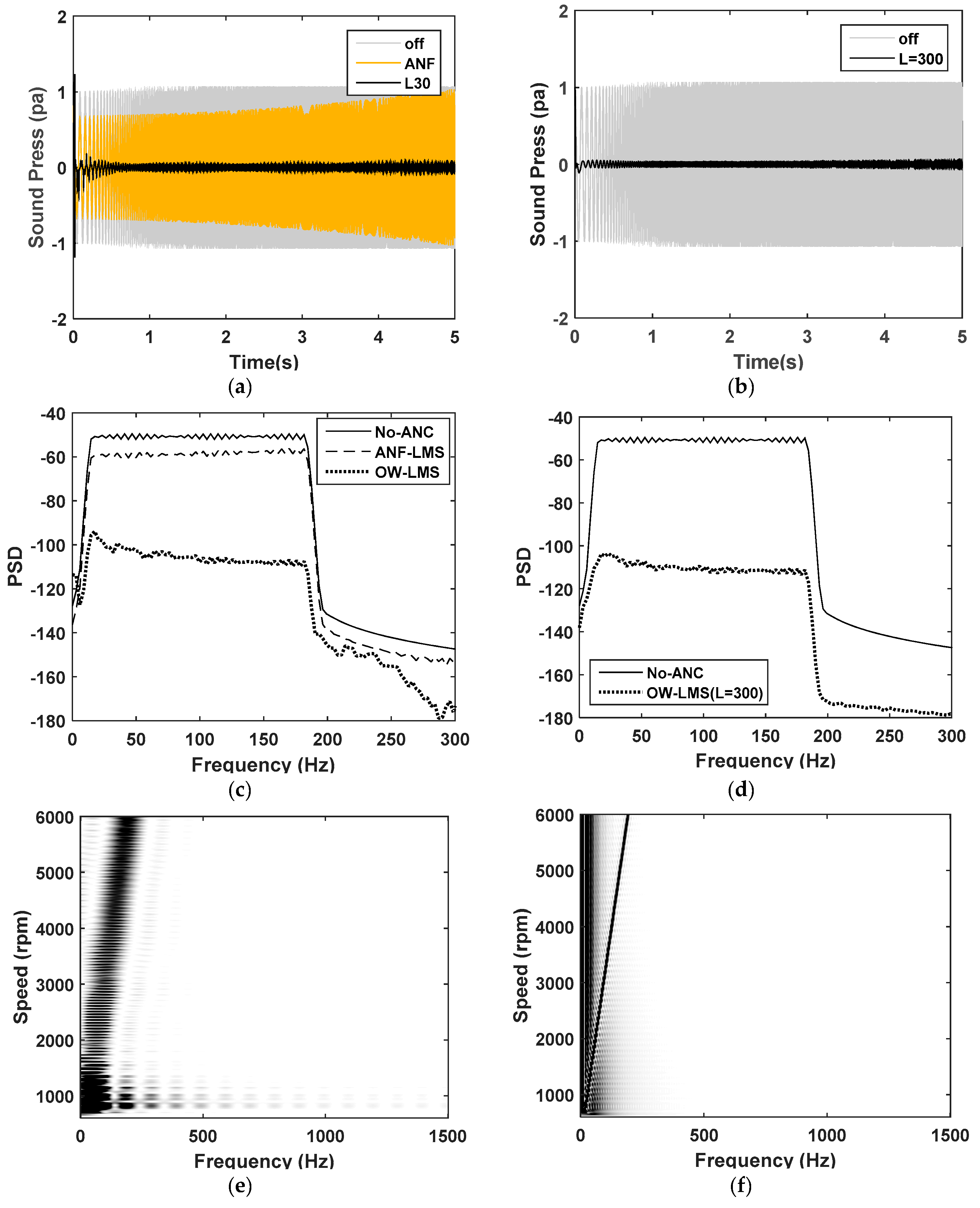
Figure 8.
Time history and PSD of signal 1 controlled by the leaky LMS-algorithm-based adaptive notch filter ( = 0.5, γ = 0.5) and the OW-LMS algorithm ( = 1). (a) Comparison between the time history of the conventional method and OW-LMS (L = 30); (b) Comparison between the time history of non-control and OW-LMS (L = 300); (c) Comparison between the PSD of conventional method and OW-LMS (L = 30); (d) Comparison between the PSD of non-control and OW-LMS (L = 300); (e) Image plot of spectrum of weight vector associated with rpm (L = 30); (f) Image plot of spectrum of weight vector associated with rpm (L = 300); (f) Spectrum of weight vector (L = 30) at 4200 rpm (h) Spectrum of weight vector (L = 300) at 4200 rpm.


Figure 9.
Simulation for signal 2 controlled by the LMS-algorithm-based adaptive notch filter and the OW-LMS algorithm. (a) Time history controlled by LMS-algorithm-based adaptive notch filter; (b) Time history controlled by OW-LMS algorithm; (c) Short-time Fourier transform (STFT) of signal 2 controlled by OW-LMS (L = 30); (d) STFT of signal 2 controlled by OW-LMS (L = 300); (e) STFT of signal 2 controlled by LMS algorithm-based adaptive notch filter; (f) Comparison of PSD of signal 2 controlled by each algorithm.

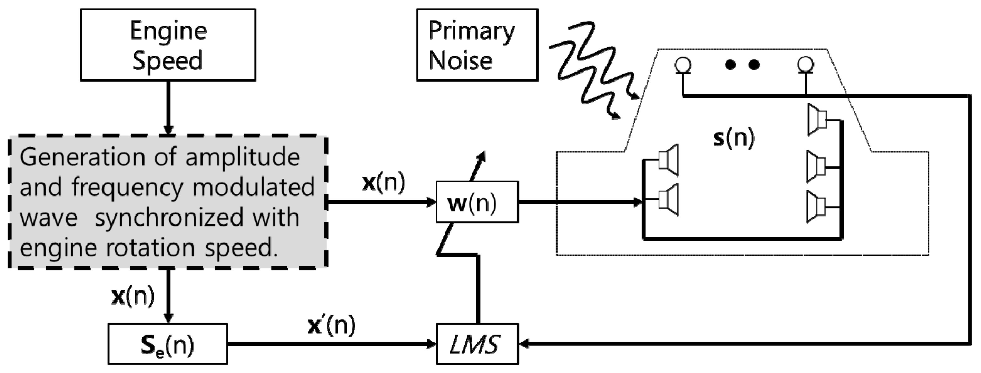
Figure 10.
Block diagram of active control of interior noise in a test vehicle based on the OW-FxLMS algorithm.
Figure 10.
Block diagram of active control of interior noise in a test vehicle based on the OW-FxLMS algorithm.

Figure 11.
Active noise cancelling system for attenuation of engine noise associated with multiple harmonic order components of the engine rotation frequency using (a) FxLMS-algorithm-based adaptive notch filter, and (b) the OW- FxLMS algorithm.
Figure 11.
Active noise cancelling system for attenuation of engine noise associated with multiple harmonic order components of the engine rotation frequency using (a) FxLMS-algorithm-based adaptive notch filter, and (b) the OW- FxLMS algorithm.

Figure 12.
Test car for the active control of interior noise (a) error microphone; (b) the secondary speaker and controller (c) controller monitor.
Figure 12.
Test car for the active control of interior noise (a) error microphone; (b) the secondary speaker and controller (c) controller monitor.

Figure 13.
Equipment in the ANC system for active control of interior noise in a test vehicle.

Figure 14.
Transfer function S(z) of the secondary path and impulse response s(n) of the secondary path. (a) Transfer function; (b) Impulse response.
Figure 14.
Transfer function S(z) of the secondary path and impulse response s(n) of the secondary path. (a) Transfer function; (b) Impulse response.

Figure 15.
Multichannel ANC algorithm with 5 subsystems used for this test based on Simulink.

Figure 16.
Comparison of sound pressure level (SPL) controlled actively by the FxLMS-algorithm-based adaptive notch filter and the OW-FxLMS algorithm at the driver seat. The driving conditions are a no-load condition and fast run-up. (a) Time history; (b) PSD; (c) Overall level of SPL; (d) SPL of the second order.

Figure 17.
Performance of the ANC system with the new algorithm. (a) Overall level; (b) Second order. The driving condition is the road condition. (Solid line: ANC off. Dotted line: ANC on.).
Figure 17.
Performance of the ANC system with the new algorithm. (a) Overall level; (b) Second order. The driving condition is the road condition. (Solid line: ANC off. Dotted line: ANC on.).

Figure 18.
Performance of the ANC system with the new algorithm for full load condition of the engine. (a) Left seat (driver seat) and (b) right seat (passenger seat) (Solid line: ANC off. Dotted line: ANC on.).
Figure 18.
Performance of the ANC system with the new algorithm for full load condition of the engine. (a) Left seat (driver seat) and (b) right seat (passenger seat) (Solid line: ANC off. Dotted line: ANC on.).


Table 1.
Pseudo code of the OW-FxLMS algorithm.
| Parameters: | Lo = Number of Taps | |
|---|---|---|
| Initial condition: | w (0) = 0 | Use Equation (16) |
| Data | ||
| (a) Given: | (n); Lo-by-1 tap input vector | |
| : Normalized sinusoidal signal | ||
| d(n): desired response at time n | : Measured impulse response of the 2nd path of the system includes electric part. | |
| Note: ⊗ means convolution | ||
| (b) To be computed: | w(n + 1) = estimate of tap-weight vector at time n + 1 | |
| Computation: | n = 0, 1, 2, … | |
© 2018 by the authors. Licensee MDPI, Basel, Switzerland. This article is an open access article distributed under the terms and conditions of the Creative Commons Attribution (CC BY) license (http://creativecommons.org/licenses/by/4.0/).
Share and Cite
MDPI and ACS Style
Lee, S.-K.; Lee, S.; Back, J.; Shin, T. A New Method for Active Cancellation of Engine Order Noise in a Passenger Car. Appl. Sci. 2018, 8, 1394. https://doi.org/10.3390/app8081394
AMA Style
Lee S-K, Lee S, Back J, Shin T. A New Method for Active Cancellation of Engine Order Noise in a Passenger Car. Applied Sciences. 2018; 8(8):1394. https://doi.org/10.3390/app8081394
Chicago/Turabian StyleLee, Sang-Kwon, Seungmin Lee, Jiseon Back, and Taejin Shin. 2018. "A New Method for Active Cancellation of Engine Order Noise in a Passenger Car" Applied Sciences 8, no. 8: 1394. https://doi.org/10.3390/app8081394
Note that from the first issue of 2016, this journal uses article numbers instead of page numbers. See further details here.