Visualization of the Strain-Rate State of a Data Cloud: Analysis of the Temporal Change of an Urban Multivariate Description

Abstract

One challenging problem is the representation of three-dimensional datasets that vary with time. These datasets can be thought of as a cloud of points that gradually deforms. However, point-wise variations lack information about the overall deformation pattern, and, more importantly, about the extreme deformation locations inside the cloud. This present article applies a technique in computational mechanics to derive the strain-rate state of a time-dependent and three-dimensional data distribution, by which one can characterize its main trends of shift. Indeed, the tensorial analysis methodology is able to determine the global deformation rates in the entire dataset. With the use of this technique, one can characterize the significant fluctuations in a reduced multivariate description of an urban system and identify the possible causes of those changes: calculating the strain-rate state of a PCA-based multivariate description of an urban system, we are able to describe the clustering and divergence patterns between the districts of a city and to characterize the temporal rate in which those variations happen.

1. Introduction

One challenging problem in data analysis is the representation of three-dimensional discrete data [1]. This analysis becomes harder when a time-dependent change of the data takes place, introducing a new temporal dimension. In the present article, we explore formal approaches to quantify the temporal change of discrete three-dimensional data. Specifically, we build a methodology to assess the transformation of a data cloud that is derived from a Principal Component Analysis (PCA): a 13-year multivariate description in [2] that provides a reduced description of an urban system given only by the first three principal components. Since the points represent an abstraction of an urban system, one main goal is to understand the temporal variation of the multivariate description of the districts in order to analyze the behavior of the overall city in the time-span. Our main hypothesis is that these three-dimensional datasets can be thought of as a cloud of points that gradually deforms.

However, the challenging issue is that deformation between consecutive times cannot be visualized accurately. There are some methods to overcome this difficulty. One is the vector plot of three-dimensional displacements or velocities, which is typically used to visualize results in computational mechanics applications [3,4,5]. For example, these methods are used in the kinematic visualization of motion [6,7,8,9,10], but they are restricted to display the relative motion among the data, and are not able to identify the most dynamic regions of the dataset. Another is the parallel coordinate technique that successfully exhibits the temporal change of highly-dimensional statistical and information datasets [11]. However, multi-dimensional data are mostly segmented into two-dimensional subsets, which are easier to deal with, Similar to the computer tomographic scans of medical imaging [1,12,13]. However, none of these methods are suitable for understanding the patterns of diversification or conformation, which are closely related to the temporal change of the differences between join data values: the maximum and minimum magnitudes of variation and the evaluation of their direction can be significantly helpful to identify differentiation patterns in the data [14]. Conversely, they can be beneficial for locating uniformity in a dataset that was previously differentiated.

One common approach to understanding the temporal change of the dataset is to use confidence ellipses in dimensionally-reduced representations (i.e., PCA) [15,16,17]. This type of approach has been applied to several time-dependent problems (e.g., [18,19,20,21]). Confidence ellipses quantify the dispersion of the results: the main directions and intervals of variance accounting for the spatiotemporal distribution are calculated first, and then, the ellipses (or ellipsoids in 3D) are drawn using those intervals as the main axes. A temporal analysis can be achieved by evaluating the geometrical characteristics of the ellipses, especially their area, to which the change of the distribution can be associated. Their main drawback lies in the failure to locate the most dynamic areas in the dataset [22].

The field of continuum mechanics provides a measure of the temporal variation of the distance in between points: the strain-rate tensor (see, for instance, [23]). The continuum mechanics theory—which arises from the classical Newtonian mechanics—analyzes the causes and effects of motion for a deformable media composed by an infinite group of particles. When a continuous media is being deformed in various directions at different rates, the strain-rate of a certain position in the medium cannot be expressed by a scalar value solely. It cannot even be expressed by using a single vector. Instead, the rate of deformation must be expressed by the rank-two strain-rate tensor with its components determined by the positional derivatives along each spatial dimension. Hence, the mathematical framework of tensors can determine exactly the deformation that is accumulated in a location inside the medium—which is typically subject to the imposition of displacements or loads. This tensor is commonly used to detail the amount of elastic energy in the physical descriptions of multiple materials, such as solids or fluids (see [24] for a complete mathematical exposition). Most of those models are formulated as the product of a constitutive tensor and the strain-rate tensor, giving the stress condition of the material that is balanced in the kinetic equations. In the present study, the calculation of the strain-rate tensor is not related to the kinetics of any material, and, thus, it can only be a mathematical tool that supports the examination of the deformation rates in the discrete statistical data.

However, the strain-rate tensor arises from the continuum assumption, and discrete displacements of points rather than continuous distributions take place in the variation of the data cloud. Typically, the issue of applying derivatives to discrete displacements of points is solved by several different approaches. Few statistical techniques use co-variance functions to represent directly the strain-rate field (see, e.g., [25]). The common approach is to compute a continuous version of the displacement—or velocity—field, so that the derivatives can be applied to the continuous displacements. Some methods in this line have interpolated the discrete displacements by minimizing the residual—or distance—between the continuous interpolation and the discrete version [26]. Other interpolation techniques weight the distance between an interpolated piece-wise continuous field and the discrete displacement field (see, e.g., [27]). This method results in a minimization technique where a continuous strain-rate field can be derived. For example, the piece-wise continuous field can be defined as being splines or the widely used linear polynomials in variational formulations [28]. These techniques have been applied in Earth science and medical imaging works [29,30,31], as well as in the strain-rate calculation of geodetic observations [32,33].

Another fundamental issue is the representation of the strain-rate state. One of the possible techniques that can help to visualize the deformation rate of the dataset is to plot the main components of the tensor using strain-rate diagrams, where concentrations of strain-rate patterns can be displayed as vector fields (see, for example, the ones in geodetical observations of the Earth’s mantle [34,35,36]). The main drawback of strain-rate diagrams is that the strain-rate components are visualized as the projection of three-dimensional vector fields into the two-dimensional framework, and, therefore, the third-dimension component has to be necessarily neglected. Another method, more suitable to two-dimensional plots, is the contour graph of principal stresses, where the stress patterns in structural elements [37,38] and tectonics [39] are visualized using continuous lines that depend on the stress magnitude. That method overcomes the three-dimensional issue, but it does not give insights about the orientation of the principal stresses. A dual form of the contour graph is to calculate the family of curves that are instantaneously tangent to the extension and contraction components of the strain-rate tensor: the so-called trajectory curves in the continuum mechanics field [23]. The trajectories of each principal component of the stress can be depicted in a separated plot with the stress magnitude colored along the trajectory line such that stress patterns are completely shown in a two-dimensional framework.

Since a robust methodology that describes the temporal change of the urban system—represented by a multivariate dataset—has not been carried out before, we perform a quantitative analysis by including the strain-rate tensor as the fundamental metric. In this work, we calculate the strain-rate state of the discrete dataset without a priori assuming the mechanisms by which the system experiences transformation. To apply the continuum mechanics principles into the discrete dataset, we use interpolation methods, such as the ones applied in discrete variational formulations (i.e., Finite Element Methods (FEM), Particle Methods, Collocation Methods, Mesh-less methods, etc.). Specifically, we derive the three-dimensional strain-rate tensor from a FEM interpolation of the discrete velocity field, as introduced in [40,41,42]. We include the trajectory lines of the principal strain-rate components as the methodology that can be used in a computational (two-dimensional) framework for visualizing the main patterns of change in any time-dependent data cloud. This approach overcomes the three-dimensional representation problem by separating the strain-rate state of the cloud in several two-dimensional plots—one for each principal component of the strain-rate—which exhibit the magnitudes and orientations of the deformation patterns.

The remaining parts of this document are organized as follows. In Section 2, the methodology to compute the discrete version of the strain-rate tensor is presented. Since the main problem involves the calculation of the derivatives of discontinuous—discrete—velocities and the visualization of the strain-rate patterns, we extensively detail the numerical techniques that are adopted in the present approach. Next, in Section 3, we present the application of the methodology to the case study—the urban system of Barcelona—by visualizing its main strain-rate patterns, meaning the city’s environmental, social and economic change. In Section 4, some conclusions of the proposed methodology close this article.

2. Methods

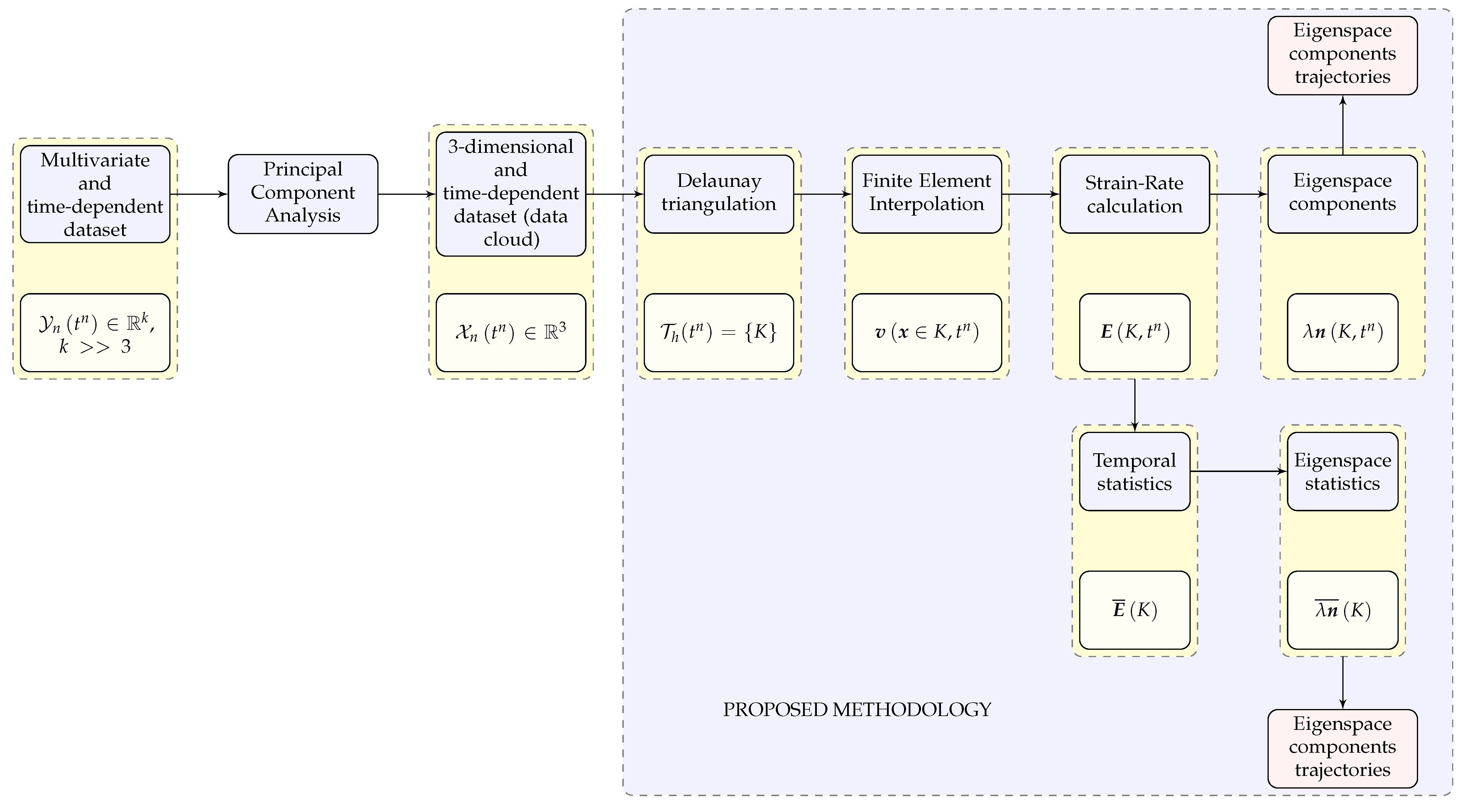
We begin this section with a review of the strain-rate tensor calculation provided a discrete three-dimensional data cloud. For doing so, the formal problem of the time-dependent dataset is introduced first. Then, we explain the numerical techniques that transform the discrete dataset into a mathematical framework by which the strain-rate tensor can be computed. Most of the ideas rely on the geometrical analysis of the discrete dataset by computing the spatial discretization of the dataset into geometric elements through a Delaunay Triangulation. After doing that, the computation of the strain-rate is performed with a FEM interpolation of the velocity field. Finally, we address the eigen-problem for the strain-rate tensor, such that the solution of the eigenvalues/eigenvectors gives the extrema strain-rates at each geometric element. The flow chart diagram of this methodology is abstracted in Figure 1, including the main outcomes of each step. The extended explanation of the methodology is developed along the present section.

2.1. Time-Dependent Three-Dimensional Dataset

Since the main objective of this work is to reveal the temporal transformation of a three-dimensional and time-dependent dataset, let us first introduce some notation in order to clarify the mathematical ideas to be used. Let us define the discrete time-dependent data to be the set of points $\mathcal{P}=\left\{p_i\right\}$, with $i=1,2,\dots ,m$, being m the total data. The values in each one of the three dimensions can be seen as scalar coefficients for a set of basis vectors. This tuple of components compose the vector that we call the position or coordinate ${\mathit{x}}_i={\left[x_{i,1}{x}_{i,2}{x}_{i,3}\right]}^{\top }$, with the superscript ⊤ denoting the transpose operation, the first subscript referring to the point i and the second to the dimension. Hence, we call ${\mathcal{X}}_n\left(t\right)=\left\{{\mathit{x}}_1\left(t\right),{\mathit{x}}_2\left(t\right),\dots ,{\mathit{x}}_i\left(t\right),\dots ,{\mathit{x}}_n\left(t\right)\right\}\in {\mathbb{R}}^3$ the positions of the points in a certain time t. Let us consider a uniform partition of the time span $t\in [t^d,t^g]$ in a sequence of discrete time-steps $t^d=t^0<t^1<\dots <t^n<\dots <t^N=t^g$, with $\delta t>0$ the time-step-size defining $t^{n+1}=t^n+\delta t$ for $n=0,1,2,\dots ,N$. Thereby, we use the superscripts to denote the discrete time-steps, with the only exception of denoting the transpose operation with the superscript ⊤.

Since the time-dependent dataset of the case study comes from a PCA reduction of a higher-dimensional multivariate dataset ${\mathcal{Y}}_n\left(t\right)=\left\{{\mathit{y}}_1\left(t\right),{\mathit{y}}_2\left(t\right),\dots ,{\mathit{y}}_i\left(t\right),\dots ,{\mathit{y}}_n\left(t\right)\right\}\in {\mathbb{R}}^k$, with $k>>3$ and $t\in [t^d,t^g]$, into a lower-dimensional one ${\mathcal{X}}_n\left(t\right)$, $t\in [t^d,t^g]$ that possesses only three independent dimensions, namely Principal Component 1 (PC1), Principal Component 2 (PC2), and Principal Component 3 (PC3), we use the Cartesian coordinate system straightforwardly with each principal component being a dimension. That is, ${\mathit{x}}_i\left(t^n\right)={\left[x_{i,\mathrm{PC}1}\left(t^n\right)x_{i,\mathrm{PC}2}\left(t^n\right)x_{i,\mathrm{PC}3}\left(t^n\right)\right]}^{\top }$. Hence, the discrete time-dependent dataset can be thought of as a cloud of points in the three-dimensional space that deforms gradually over time.

2.2. Finite Element Method Interpolation

The main idea of the present approach is to transform the discrete cloud of points into a mathematical framework—similar to a deformable medium—by which the strain-rate tensor can be computed. To do so, we generate a mesh ${\mathcal{T}}_h\left(t\right)=\left\{K\right\}$ from the set of points $\mathcal{P}$ that is composed of non-overlapping and conforming geometrical elements K of diameter h. There are several methods to generate a mesh from a set of points, all which are studied in the computational geometry field [43]. Here, we apply Delaunay triangulation $DT\left(\mathcal{P}\right)$ for several reasons: (1) the aspect ratio of the triangulated elements produce a high-quality mesh; and (2) fast Delaunay triangulation algorithms have been developed recently (see, for example, the one in [44]).

The result of applying the Delaunay triangulation over the set of points is a discrete mesh ${\mathcal{T}}_h:=DT\left(\mathcal{P}\right)$ that possess the following characteristics: it covers exactly the convex hull $\Omega$ of the point set, no point $p_i$ is isolated from the triangulation, and all the elements $\left\{K\right\}$ are four-point tetrahedrons, which are completely defined by the position of their four corner points $K:=\left\{{\mathit{x}}_j\right\}$, with $j=1,2,3,4$. The generated mesh ${\mathcal{T}}_h=DT\left(\mathcal{P}\right)$ can be seen as a—material—domain $\Omega$ that suffers deformations from the displacements of the points between consecutive time-steps. Since only discrete displacements between consecutive time-steps are known for the set of points, we now explain how the continuous velocity field inside the mesh is calculated.

Even though the FEM has been used to perform interpolation using the point-wise data (see [41,42] for applications in one and two-dimensional data), in this work, we apply this well-known method in a three-dimensional setting. In FEM, the finite interpolating space ${\mathcal{V}}_h$ is defined as made of continuous piece-wise polynomials $N\left(\mathit{x}\right)$ in the mesh ${\mathcal{T}}_h$, where the discrete approximation ${\mathit{F}}_h(\mathit{x},t)\in {\mathcal{V}}_h$ of any multi-dimensional function $\mathit{F}(\mathit{x},t)$, $\mathit{x}\in \Omega$, can be written as

$$\begin{array}{ccc}\hfill \mathit{F}(\mathit{x},t)\approx & {\mathit{F}}_h(\mathit{x},t):=\sum _{i=1}^{n}N\left({\mathit{x}}_i\right){\mathit{F}}_i\left(t\right),\hfill & \mathit{x}\in \Omega .\hfill \end{array}$$

(1)

We use the simplest finite element: the tetrahedron with linear polynomials and four nodes. Again, some notation is required to define the polynomials inside the element. The set of normalized coordinates ${\eta }_1,{\eta }_2,{\eta }_3,{\eta }_4$ in each tetrahedron K is such that the value of ${\eta }_i$ is one at the point $p_i\in K$, zero at the other three corner points, and varies linearly from that point to the opposite edges. This set of coordinates has the property that the sum of the four coordinates (each belonging to one tetrahedron point) in any location inside the tetrahedron is identically one: ${\eta }_1\left({\mathit{x}}_i\right)+{\eta }_2\left({\mathit{x}}_i\right)+{\eta }_3\left({\mathit{x}}_i\right)+{\eta }_4\left({\mathit{x}}_i\right)=1$, with ${\mathit{x}}_i\in K$. Hence, the shape functions inside each linear tetrahedron are defined to be these coordinates: $N_i\left({\mathit{x}}_i\right)={\eta }_i\left({\mathit{x}}_i\right)$, with $i=1,2,3,4$ denoting the corner points. The FEM interpolation in Equation (1) of a three-dimensional vector function, e.g. $\mathit{F}\left(\mathit{x},t\right)$, can be defined inside each linear tetrahedron K as

$$\begin{array}{cc}\hfill \mathit{F}\left(\mathit{x},t\right)={\eta }_1\left(\mathit{x}\right){\mathit{F}}_1\left(t\right)+{\eta }_2\left(\mathit{x}\right){\mathit{F}}_2\left(t\right)+{\eta }_3\left(\mathit{x}\right){\mathit{F}}_3\left(t\right)+{\eta }_4\left(\mathit{x}\right){\mathit{F}}_4\left(t\right)=\sum _{j=1}^4{\eta }_j\left(\mathit{x}\right){\mathit{F}}_j\left(t\right),& \hfill \mathit{x}\in K,\end{array}$$

(2)

by denoting ${\mathit{F}}_i\left(t\right)=\mathit{F}\left({\mathit{x}}_i,t\right)$, for $i=1,2,3,4$, nodes of the tetrahedron.

The way the tetrahedral coordinates ${\eta }_i$, $i=1,2,3,4$, are defined is by means of the previous interpolating relation together with the summation constraint. That is, when one aims to define the tetrahedron geometry and calculate any position inside the tetrahedron $\mathit{x}={\left[x_1{x}_2{x}_3\right]}^{\top }$, we compute

$$\begin{array}{c}\hfill \left[\begin{array}{c}1\\ x_1\\ x_2\\ x_3\end{array}\right]=\left[\begin{array}{cccc}1& 1& 1& 1\\ x_{1,1}& x_{2,1}& x_{3,1}& x_{4,1}\\ x_{1,2}& x_{2,2}& x_{3,2}& x_{4,2}\\ x_{1,3}& x_{2,3}& x_{3,3}& x_{4,3}\end{array}\right]\left[\begin{array}{c}{\eta }_1\left(\mathit{x}\right)\\ {\eta }_2\left(\mathit{x}\right)\\ {\eta }_3\left(\mathit{x}\right)\\ {\eta }_4\left(\mathit{x}\right)\end{array}\right]\therefore \left[\begin{array}{c}{\eta }_1\left(\mathit{x}\right)\\ {\eta }_2\left(\mathit{x}\right)\\ {\eta }_3\left(\mathit{x}\right)\\ {\eta }_4\left(\mathit{x}\right)\end{array}\right]=\frac{1}{6\upsilon }\left[\begin{array}{cccc}6\upsilon & a_1& b_1& c_1\\ 6\upsilon & a_2& b_2& c_2\\ 6\upsilon & a_3& b_3& c_3\\ 6\upsilon & a_4& b_1& c_4\end{array}\right]\left[\begin{array}{c}1\\ x_1\\ x_2\\ x_3\end{array}\right]\end{array}$$

(3)

in order to obtain the tetrahedral coordinates system where the coefficients of the inverted matrix are given by

$$\begin{array}{cccccc}\hfill a_1& =x_{2,2}{x}_{43,3}-x_{3,2}{x}_{42,3}+x_{4,2}{x}_{32,3},\hfill & \hfill b_1& =-x_{2,1}{x}_{43,3}+x_{3,1}{x}_{42,3}-x_{4,1}{x}_{32,3},\hfill & \hfill c_1& =x_{2,1}{x}_{43,2}-x_{3,1}{x}_{42,2}+x_{4,1}{x}_{32,2},\hfill \\ \hfill a_2& =-x_{1,2}{x}_{43,3}+x_{3,2}{x}_{41,3}-x_{4,2}{x}_{31,3},\hfill & \hfill b_2& =x_{1,1}{x}_{43,3}-x_{3,1}{x}_{41,3}+x_{4,1}{x}_{31,3},\hfill & \hfill c_1& =-x_{1,1}{x}_{43,2}+x_{3,1}{x}_{41,2}-x_{4,1}{x}_{31,2},\hfill \\ \hfill a_3& =x_{1,2}{x}_{42,3}-x_{2,2}{x}_{41,3}+x_{4,2}{x}_{21,3},\hfill & \hfill b_3& =-x_{1,1}{x}_{42,3}+x_{2,1}{x}_{41,3}-x_{4,1}{x}_{21,3},\hfill & \hfill c_3& =x_{1,1}{x}_{42,2}-x_{2,1}{x}_{41,2}+x_{4,1}{x}_{21,2},\hfill \\ \hfill a_4& =-x_{1,2}{x}_{32,3}+x_{2,2}{x}_{31,3}-x_{3,2}{x}_{21,3},\hfill & \hfill b_4& =x_{1,1}{x}_{32,3}-x_{2,1}{x}_{31,3}+x_{3,1}{x}_{21,3},\hfill & \hfill c_4& =-x_{1,1}{x}_{32,2}+x_{2,1}{x}_{31,2}-x_{3,1}{x}_{21,2}.\hfill \end{array}$$

Here, the abbreviation ${\mathit{x}}_{ij}={\mathit{x}}_i-{\mathit{x}}_j$ is used, and the volume $\upsilon$ can be calculated with the expression

$$\begin{array}{cc}\hfill 6\upsilon =& x_{21,1}\left(x_{31,2}{x}_{41,3}-x_{41,2}{x}_{31,3}\right)+x_{21,2}\left(x_{41,1}{x}_{31,3}-x_{31,1}{x}_{41,3}\right)+x_{21,3}\left(x_{31,1}{x}_{41,2}-x_{41,1}{x}_{31,2}\right).\hfill \end{array}$$

At this point, it is possible to calculate the spatial derivatives of any interpolated function $\frac{\partial }{\partial \mathit{x}}\mathit{F}\left(\mathit{x},t\right)$ in terms of the tetrahedral coordinates as

$$\begin{array}{ccc}\hfill \frac{\partial \mathit{F}\left(\mathit{x},t\right)}{\partial \mathit{x}}& =\left[\begin{array}{c}\frac{\partial \mathit{F}\left(\mathit{x},t\right)}{\partial x_1}\\ \frac{\partial \mathit{F}\left(\mathit{x},t\right)}{\partial x_2}\\ \frac{\partial \mathit{F}\left(\mathit{x},t\right)}{\partial x_3}\end{array}\right]=\sum _{j=1}^4\left[\begin{array}{c}\frac{\partial \mathit{F}\left(\mathit{x},t\right)}{\partial {\eta }_j}\frac{\partial {\eta }_j}{\partial x_1}\\ \frac{\partial \mathit{F}\left(\mathit{x},t\right)}{\partial {\eta }_j}\frac{\partial {\eta }_j}{\partial x_2}\\ \frac{\partial \mathit{F}\left(\mathit{x},t\right)}{\partial {\eta }_j}\frac{\partial {\eta }_j}{\partial x_3}\end{array}\right]=\sum _{j=1}^4\left[\begin{array}{c}\frac{1}{6\upsilon }\frac{\partial \mathit{F}\left(\mathit{x},t\right)}{\partial {\eta }_j}{a}_j\\ \frac{1}{6\upsilon }\frac{\partial \mathit{F}\left(\mathit{x},t\right)}{\partial {\eta }_j}{b}_j\\ \frac{1}{6\upsilon }\frac{\partial \mathit{F}\left(\mathit{x},t\right)}{\partial {\eta }_j}{c}_j\end{array}\right],\hfill & \mathit{x}\in K.\hfill \end{array}$$

(4)

The way to calculate the continuous stress-rate tensor field is through the derivation of a continuous version of the velocities. Hence, we calculate the continuous velocity field by means of the FEM, in which linear piece-wise polynomials are used to interpolate the velocity at any spatial position inside the mesh. First, let us explain how to calculate the discrete version of the velocity from the cloud of points. We suppose that the displacement ${\mathit{s}}_i$ of point $p_i$ in the time interval $\left(t^n,t^{n+1}\right)$ can be defined—without loss of accuracy—as infinitesimal, in the sense of ${\mathit{s}}_i\left(t^n\right)\approx {\mathit{x}}_i\left(t^{n+1}\right)-{\mathit{x}}_i\left(t^n\right)$. With this supposition in hand, we use the Taylor expansion:

$$\begin{array}{cc}\hfill {\mathit{x}}_i\left(t\right)=& \sum _{k=1}^{\infty }\frac{\delta t^k}{k!}{\left.\frac{d^k{\mathit{x}}_i}{d{t}^k}\right|}_{t=t_o}={\mathit{x}}_i\left(t_0\right)+{\left.\frac{d{\mathit{x}}_i}{dt}\right|}_{t=t_o}\delta t+{\left.\frac{d^2{\mathit{x}}_i}{d{t}^2}\right|}_{t=t_o}\frac{\delta t^2}{2}+\cdots ,\hfill \end{array}$$

(5)

in order to calculate the discrete velocity ${\mathit{v}}_i$ of point $p_i$ as

$$\begin{array}{cc}\hfill {\mathit{v}}_i\left(t^n\right)={\left.\frac{d{\mathit{x}}_i}{dt}\right|}_{t=t^n}\approx \frac{{\mathit{x}}_i\left(t^{n+1}\right)-{\mathit{x}}_i\left(t^n\right)}{\delta t}=& \frac{{\mathit{x}}_i\left(t^{n+1}\right)-{\mathit{x}}_i\left(t^n\right)}{\left(t^{n+1}-t^n\right)},\hfill \end{array}$$

(6)

where the second (and higher) order terms are neglected. The previous result then generates the continuous version of velocity by replacing it in Equation (2).

2.3. Elemental Strain-Rate Calculation

Having defined the continuous space of velocities, we can calculate the derivatives along each of the spatial directions and derive the strain-rate tensor field.

Following the continuum mechanics concepts in [23] and assuming small deformations, the strain-rate tensor is calculated as

$$\begin{array}{cc}\hfill \mathit{E}\left(\mathit{x},t^n\right):=& \frac{1}{2}\left(\nabla \mathit{v}\left(\mathit{x},t^n\right)+{\left(\nabla \mathit{v}\left(\mathit{x},t^n\right)\right)}^{\top }\right),\hfill \end{array}$$

with $\nabla \mathit{v}$ the gradient of velocity. Each component of the $3\times 3$-tensor is developed in Cartesian coordinates as

$$\begin{array}{cc}\hfill \left[\begin{array}{ccc}{E}_{11}& E_{12}& E_{13}\\ E_{21}& E_{22}& E_{23}\\ E_{31}& E_{32}& E_{33}\end{array}\right]=& \left[\begin{array}{ccc}\frac{\partial v_1\left(\mathit{x},t^n\right)}{\partial x_1}& \frac{1}{2}\left(\frac{\partial v_1\left(\mathit{x},t^n\right)}{\partial x_2}+\frac{\partial v_2\left(\mathit{x},t^n\right)}{\partial x_1}\right)& \frac{1}{2}\left(\frac{\partial v_1\left(\mathit{x},t^n\right)}{\partial x_3}+\frac{\partial v_3\left(\mathit{x},t^n\right)}{\partial x_1}\right)\\ \frac{1}{2}\left(\frac{\partial v_2\left(\mathit{x},t^n\right)}{\partial x_1}+\frac{\partial v_1\left(\mathit{x},t^n\right)}{\partial x_2}\right)& \frac{\partial v_2\left(\mathit{x},t^n\right)}{\partial x_2}& \frac{1}{2}\left(\frac{\partial v_2\left(\mathit{x},t^n\right)}{\partial x_3}+\frac{\partial v_3\left(\mathit{x},t^n\right)}{\partial x_2}\right)\\ \frac{1}{2}\left(\frac{\partial v_3\left(\mathit{x},t^n\right)}{\partial x_1}+\frac{\partial v_1\left(\mathit{x},t^n\right)}{\partial x_3}\right)& \frac{1}{2}\left(\frac{\partial v_3\left(\mathit{x},t^n\right)}{\partial x_2}+\frac{\partial v_2\left(\mathit{x},t^n\right)}{\partial x_3}\right)& \frac{\partial v_3\left(\mathit{x},t^n\right)}{\partial x_3}\end{array}\right].\hfill \end{array}$$

Moreover, the six independent components of the strain-rate tensor can be arranged using Voigt’s notation into a six-component strain-rate vector as follows:

$$\begin{array}{cc}\hfill \mathit{E}\left(\mathit{x},t^n\right)=& {\left[\begin{array}{cccccc}{E}_{11}\left(\mathit{x},t^n\right)& E_{22}\left(\mathit{x},t^n\right)& E_{33}\left(\mathit{x},t^n\right)& {\gamma }_{12}\left(\mathit{x},t^n\right)& {\gamma }_{23}\left(\mathit{x},t^n\right)& {\gamma }_{31}\left(\mathit{x},t^n\right)\end{array}\right]}^{\top },\hfill \end{array}$$

(7)

where ${\gamma }_{12}\left(\mathit{x},t\right)=2E_{12}\left(\mathit{x},t\right),{\gamma }_{23}\left(\mathit{x},t\right)=2E_{23}\left(\mathit{x},t\right)$ and ${\gamma }_{13}\left(\mathit{x},t\right)=2E_{13}\left(\mathit{x},t\right)$ are the shear-rate strains. With this notation in hand, the strain-rate tensor can be calculated as

$$\begin{array}{cc}\hfill \mathit{E}\left(\mathit{x},t^n\right)=\left[\begin{array}{c}{E}_{11}\left(\mathit{x},t^n\right)\\ E_{22}\left(\mathit{x},t^n\right)\\ E_{33}\left(\mathit{x},t^n\right)\\ {\gamma }_{12}\left(\mathit{x},t^n\right)\\ {\gamma }_{23}\left(\mathit{x},t^n\right)\\ {\gamma }_{31}\left(\mathit{x},t^n\right)\end{array}\right]=& \left[\begin{array}{ccc}\frac{\partial }{\partial x_1}& 0& 0\\ 0& \frac{\partial }{\partial x_2}& 0\\ 0& 0& \frac{\partial }{\partial x_3}\\ \frac{\partial }{\partial x_2}& \frac{\partial }{\partial x_1}& 0\\ 0& \frac{\partial }{\partial x_3}& \frac{\partial }{\partial x_2}\\ \frac{\partial }{\partial x_3}& 0& \frac{\partial }{\partial x_1}\end{array}\right]\left[\begin{array}{c}{v}_1\left(\mathit{x},t^n\right)\\ v_2\left(\mathit{x},t^n\right)\\ v_3\left(\mathit{x},t^n\right)\end{array}\right],\hfill \end{array}$$

(8)

by defining the matrix operator of derivatives over the velocity field. In the case of the right hand side velocities, we can arrange a node-wise vector of discrete velocities in the tetrahedron K, as

$$\begin{array}{cc}\hfill \mathit{V}\left(K,t^n\right)=& {\left[\begin{array}{cccccccc}{v}_{1,1}\left(t^n\right)& v_{1,2}\left(t^n\right)& v_{1,3}\left(t^n\right)& v_{2,1}\left(t^n\right)& v_{2,2}\left(t^n\right)& \dots & v_{4,2}\left(t^n\right)& v_{4,3}\left(t^n\right)\end{array}\right]}^{\top }.\hfill \end{array}$$

Using the definition of the finite element interpolation of any function in Equation (2) together with its partial derivatives in Equation (4), and replacing those in Equation (8), we obtain

$$\begin{array}{c}\hfill \mathit{E}\left(\mathit{x},t^n\right)=\frac{1}{6\upsilon }\sum _{j=1}^4\left[\begin{array}{ccc}{a}_j\frac{\partial }{\partial {\eta }_j}& 0& 0\\ 0& b_j\frac{\partial }{\partial {\eta }_j}& 0\\ 0& 0& c_j\frac{\partial }{\partial {\eta }_j}\\ b_j\frac{\partial }{\partial {\eta }_j}& a_j\frac{\partial }{\partial {\eta }_j}& 0\\ 0& c_j\frac{\partial }{\partial {\eta }_j}& b_j\frac{\partial }{\partial {\eta }_j}\\ c_j\frac{\partial }{\partial {\eta }_j}& 0& a_j\frac{\partial }{\partial {\eta }_j}\end{array}\right]\left[\begin{array}{c}{\eta }_j\left(\mathit{x}\right)V_{j,1}\left(t^n\right)\\ {\eta }_j\left(\mathit{x}\right)V_{j,2}\left(t^n\right)\\ {\eta }_j\left(\mathit{x}\right)V_{j,3}\left(t^n\right)\end{array}\right].\end{array}$$

(9)

Now, the operation $\frac{\partial {\eta }_i}{\partial {\eta }_j}{F}_j=F_i$ since $\frac{\partial {\eta }_i}{\partial {\eta }_j}={\delta }_{ij}$, with ${\delta }_{ij}$ the Kronecker delta. Hence, $\mathit{E}\left(K,t^n\right)$ can be calculated as the product of the matrix $\mathrm{S}\left(K\right)$ and the vector $\mathit{V}\left(K,t^n\right)$. That is,

$$\begin{array}{c}\hfill \mathit{E}\left(K,t^n\right)=\mathrm{S}\left(K,t^n\right)\mathit{V}\left(K,t^n\right),\end{array}$$

(10)

with $\mathit{x}\in K$ and the discrete matrix $\mathrm{S}\left(K,t^n\right)$ defined as

$$\begin{array}{c}\hfill \mathrm{S}\left(K,t^n\right)=\frac{1}{6\upsilon }\left[\begin{array}{cccccccccccc}{a}_1& 0& 0& a_2& 0& 0& a_3& 0& 0& a_4& 0& 0\\ 0& b_1& 0& 0& b_2& 0& 0& b_3& 0& 0& b_4& 0\\ 0& 0& c_1& 0& 0& c_2& 0& 0& c_3& 0& 0& c_4\\ b_1& a_1& 0& b_2& a_2& 0& b_3& a_3& 0& b_4& a_4& 0\\ 0& c_1& b_1& 0& c_2& b_2& 0& c_3& b_3& 0& c_4& b_4\\ c_1& 0& a_1& c_2& 0& a_2& c_3& 0& a_3& c_4& 0& a_4\end{array}\right].\end{array}$$

(11)

Thus, this last matrix can be computed solely in terms of the coordinates of the nodes.

2.4. Principal Strain-Rates

Up to this point, we have demonstrated how to calculate the elemental strain-rate. Now, our purpose is to identify the data cloud transformation throughout the visualization of the strain-rate patterns. That is, we need to identify the extrema strain-rates and their orientations. In a formal sense, this is the well-known eigenvalues and eigenvectors problem, which is stated as: if T is a linear transformation from a vector space V over a field F into itself, and v is a vector in V that is not the zero vector, then v is an eigenvector of T if $T\left(v\right)$ is a scalar multiple of v. Knowing that by definition the second-order strain-rate tensor is a linear operator from a vector field into another first-order tensor field, the previous definition applied to the strain-rate tensor leads to:

$$\begin{array}{cc}\hfill \left[\mathit{E}\left(K,t^n\right)-\mathit{I}\lambda \left(K,t^n\right)\right]\mathit{n}\left(K,t^n\right)=& 0,\hfill \end{array}$$

(12)

where $\mathit{I}$ is the $3\times 3$ identity tensor; $\mathit{n}\left(K,t^n\right)\in {\mathbb{R}}^3$ is a normalized (non zero), i.e., unit, vector called eigenvector; and $\lambda \left(K,t^n\right)\in \mathbb{R}$ is the eigenvalue associated with the eigenvector. In other words, an eigenvector is a vector that changes by only a scalar factor when the strain-rate tensor is applied to it, resulting in a vector parallel to itself. By solving Equation (12) ,one obtains three different eigenvalues ${\lambda }_1\left(K,t^n\right),{\lambda }_2\left(K,t^n\right),{\lambda }_3\left(K,t^n\right),$ and three eigenvectors ${\mathit{n}}_1\left(K,t^n\right),{\mathit{n}}_2\left(K,t^n\right),{\mathit{n}}_3\left(K,t^n\right),$ associated with each eigenvalue.

The eigenvalues and eigenvectors describe the principal magnitudes and orientations of the strain-rate tensor: since the diagonal components of the strain-rate tensor $E_{11}\left(K,t^n\right),E_{22}\left(K,t^n\right),$ and $E_{33}\left(K,t^n\right)$ have different values in different reference systems, one finds with the set of eigenvalues the extreme—maximum and minimum—possible values that any of these components may take. Indeed, the maximum and minimum stress-rates—and their orientations—are related to the maximum and minimum eigenvalues. In this work, we follow the notation in which positive values for the eigenvalues represent the extension-rate and negative values represent contraction-rate. Hence, ${\lambda }_1\left(K,t^n\right)$ is the maximum and positive eigenvalue meaning extension-rate, ${\lambda }_3\left(K,t^n\right)$ is the minimum and negative eigenvalue meaning contraction-rate, and ${\lambda }_2\left(K,t^n\right)$ is either extension or contraction rate, but in smaller magnitude.

Hence, with the extrema strain-rates at the elemental level, we can reveal the deformation trend of the data cloud, and, above all, locating which regions suffer the most abrupt change in the time-span. We also propose to draw the family of curves—trajectories—that are instantaneously tangent to ${\lambda }_1{\mathit{n}}_1\left(K,t^n\right),{\lambda }_2{\mathit{n}}_2\left(K,t^n\right),$ and ${\lambda }_3{\mathit{n}}_3\left(K,t^n\right)$ in the complete mesh $\Omega$. This results in a graph plot for each of the $\lambda \mathit{n}\left(K,t^n\right)$ fields that can be easily represented in a two-dimensional framework. These tangent lines can be colored according to the eigenvalue magnitude such that they completely illustrate the main patterns of change inside the data cloud. Note, nevertheless, that $\lambda \mathit{n}\left(K,t^n\right)$ is a composition of a vector using tensor components. Those differ in formal definition, but we use this concept merely for visualization purposes.

Nevertheless, we also perform some temporal statistics of the strain-rate states, where the principal strain-rates for each time-step ${\lambda }_i{\mathit{n}}_i\left(K,t^n\right)$ are accounted as the temporal events: each strain-rate state is accounted as a single observation. Specifically, we calculate the time-average of the eigenspace components $\overline{{\lambda }_i}\left(K\right)$ and $\overline{{\mathit{n}}_i}\left(K\right)$, the maximum extension-rate in the time span $L^{\infty }\left({\lambda }_1\left(K\right)\right)$, and the maximum contraction-rate in the time span $L^{-\infty }\left({\lambda }_3\left(K\right)\right)$. In this way, we calculate representative deformation results for the complete temporal interval of analysis, as well as the location of extreme values. Besides, trajectory lines can be plotted using these statistical results.

3. Results

In the present section, we demonstrate the application of this methodology to quantify the temporal change of an urban multivariate system First, we cite the case study that includes the multivariate description of the ten districts of Barcelona, and whose reduced three-dimensional dataset is used as the starting point. Then, we derive the strain-rate state of the dataset, pursuing the extension and contraction patterns visualization. Finally, we close this section with insights about the city transformation implied in the strain-rate state of the data cloud.

3.1. Time-Dependent Data Cloud from an Urban Multivariate Description

The time-dependent data cloud comes from the PCA output of a multivariate description of the city of Barcelona in [2]. Since 1987, the city has been divided into 10 administrative districts, which are the largest territorial units of the city and can be compared with neighborhoods in a common metropolitan area: Ciutat Vella, Eixample, Gràcia, Les Corts, Sarria, Sant Andreu, Sant Marti, Horta, Sants, and Nou Barris. Barcelona has a population of approximately 1.6 million inhabitants living in 10,216 ha. The inclusion of all 10 districts in the multivariate description was aimed at representing the city at its overall scale and allowing comparisons between them.

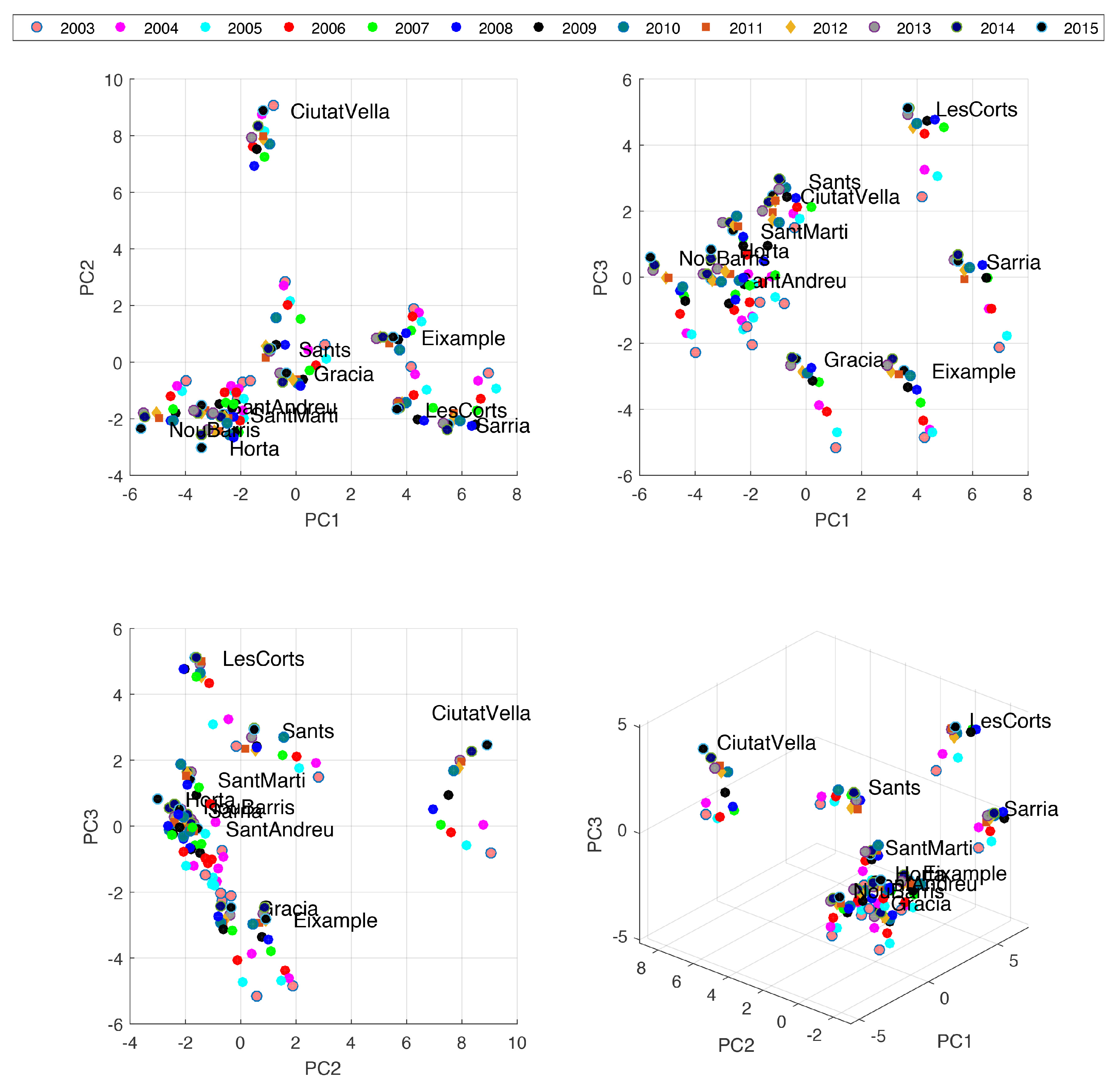
The raw multivariate description—from which the PCA is calculated—comprises the data of 40 environmental, economic, and social indicators for the ten districts in the time span of $t^0=2003\le t^n\le 2015=t^N$, $n=0,1,\dots ,12$. Hence, the case study data cloud comes from a PCA reduction of the higher-dimensional multivariate dataset ${\mathcal{Y}}_n\left(t^n\right)\in {\mathbb{R}}^{40}$, into a lower-dimensional one ${\mathcal{X}}_n\left(t^n\right)\in {\mathbb{R}}^3$ that possesses only three independent dimensions: PC1, PC2, and PC3. The dimensionally-reduced dataset from the application of the PCA is presented in Appendix A. Hence, the three-dimensional and time-dependent data cloud is composed of the coordinates ${\mathcal{X}}_n\left(t^n\right)$ of the ten $p_i$ points defined in the sequence of $N=12$ time-steps from 2003 to 2015, with the time-step size of $\delta t=1$ year. These points are displayed in Figure 2, where all observations—districts each year—in the time-span are included.

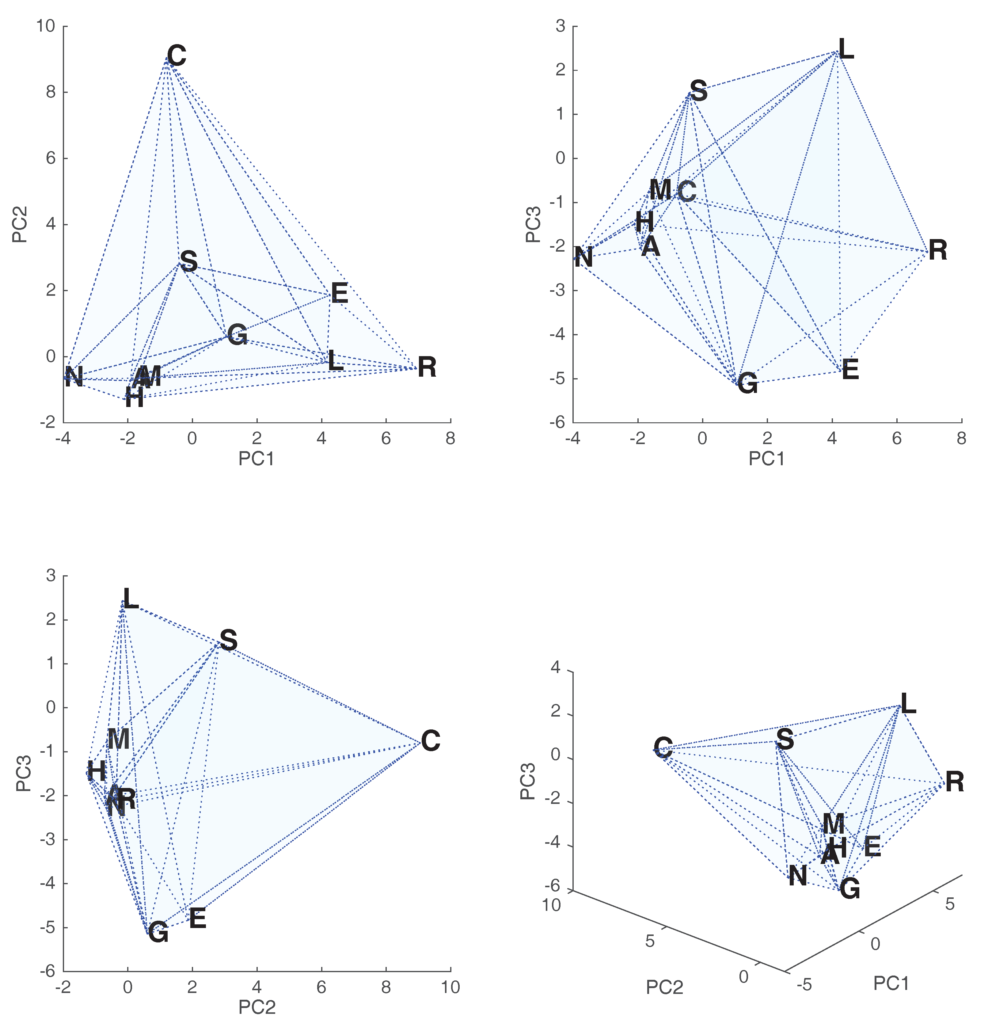
As the first step of our methodology, we applied Delaunay Triangulation (DT) to the data cloud. Specifically, we calculated the DT to the set of coordinates at each time-step ${\mathcal{X}}_n\left(t^n\right)$. This resulted in a mesh ${\mathcal{T}}_h\left(t^n\right)$ composed of $nel=\left|K\right|$ non-overlapping tetrahedrons.

Table 1. Tetrahedral elements derived from the Delaunay Triangulation of the set of points.

Element (id)	First Vertex	Second Vertex	Third Vertex	Fourth Vertex
1	Eixample	LesCorts	Gracia	Sarria
2	SantAndreu	Horta	SantMarti	NouBarris
3	Sants	SantAndreu	SantMarti	NouBarris
4	LesCorts	Eixample	Sants	CiutatVella
5	Gracia	SantMarti	Horta	Sarria
6	Gracia	SantMarti	Sarria	LesCorts
7	Eixample	Gracia	Sants	CiutatVella
8	CiutatVella	SantAndreu	Sants	NouBarris
9	Sarria	SantMarti	Horta	LesCorts
10	Gracia	SantAndreu	Sants	CiutatVella
11	Gracia	SantAndreu	CiutatVella	NouBarris
12	Sarria	Eixample	LesCorts	CiutatVella
13	Horta	SantAndreu	Gracia	NouBarris
14	SantAndreu	SantMarti	Horta	Gracia
15	LesCorts	Eixample	Gracia	Sants
16	LesCorts	Gracia	SantMarti	Sants
17	Gracia	SantAndreu	SantMarti	Sants

expands the resulting triangulation for year 2003, with the vertices information for the $nel=17$ tetrahedrons. This triangulation is also depicted in Figure 3, where the following notation for the districts in the vertices is used: C is Ciutat Vella, E is Eixample, G is Gracia, H is Horta, L is Les Corts, N is Nou Barris, A is Sant Andreu, M is Sant Martí, S is Sants, and R is Sarria. Since the position ${\mathit{x}}_i\left(t^n\right)$ of a given point $p_i$ at a later time-step can surpass the initial tetrahedron’s circumscribed sphere, we recalculated the mesh triangulation at each time step $t^n$, $n=1,\dots ,11$.

3.2. Principal Strain-Rates

We computed the strain-rate tensor of each tetrahedron with the interpolated version of the velocities for the case study, such that linear piece-wise polynomial functions defined inside each tetrahedron were used in the FEM interpolation. Certainly, we supposed that the velocities came from an infinitesimal analysis, in which the higher-order terms of the displacement were neglected. The gradients inside each tetrahedron were also considered to be constant since the polynomial functions were of first order. Applying Equation (10), we computed the strain-rate tensor of every tetrahedron, $\mathit{E}(K,t^n)$ for time-steps $n=0,\dots ,11$. Note that displacements could not be calculated for the last year $t^{12}=2015$, and that the strain-rate tensor units are year⁻¹ (for the case study).

We were interested in the magnitude and orientations of the principal strain-rates—extension and contraction—at the elemental level. Hence, the next step was to solve Equation (12) and obtain the eigenspace components (eigenvalues and eigenvectors) of the strain-rate tensor. For the sake of conciseness, we list in

Table 2. Principal strain-rate components. Eigenvalues and eigenvectors of the strain-rate tensor in the year 2003. The extension is denoted by the maximum eigenvalue ${\lambda }_1$, and contraction is denoted by the minimum eigenvalue ${\lambda }_3$.

Element (id)	${\mathit{\lambda }}_{\mathbf{1}}$ (year−1)	${\mathit{\lambda }}_{\mathbf{2}}$ (year−1)	${\mathit{\lambda }}_{\mathbf{3}}$ (year−1)	${\mathit{n}}_{\mathbf{1}}^{\mathbf{\top }}$	${\mathit{n}}_{\mathbf{2}}^{\mathbf{\top }}$	${\mathit{n}}_{\mathbf{3}}^{\mathbf{\top }}$
1	0.53152326	0.03372761	−0.5035305	[−0.4030 −0.7620 0.5069]	[−0.8521 0.1104 −0.5116]	[0.3339 −0.6381 −0.6938]
2	0.82703046	−0.07233917	−3.26208499	[0.0599 0.4379 0.8970]	[0.9979 −0.0488 −0.0428]	[0.0250 0.8977 −0.4399]
3	1.86537595	0.0239402	−1.26311701	[−0.2846 −0.7630 0.5804]	[0.8705 0.0479 0.4898]	[−0.4015 0.6447 0.6505]
4	0.13368209	0.03257601	−0.09645259	[0.3448 0.0267 0.9383]	[0.6847 −0.6909 −0.2320]	[0.6421 0.7225 −0.2565]
5	0.49758344	0.15637449	−0.04820077	[−0.2529 0.9667 0.0396]	[−0.3025 −0.1179 0.9458]	[0.9190 0.2272 0.3223]
6	0.95472589	0.0373597	−0.54006708	[−0.0595 −0.8341 0.5484]	[0.9779 0.0616 0.1998]	[−0.2005 0.5482 0.8120]
7	0.24389104	−0.02462416	−0.21220276	[0.9802 −0.0490 −0.1918]	[0.0873 0.9766 0.1964]	[0.1777 −0.2093 0.9616]
8	0.04516871	−0.00558049	−0.29509916	[−0.5143 −0.5503 −0.6578]	[0.7221 −0.6916 0.0139]	[0.4626 0.4679 −0.7531]
9	0.83841605	0.06226881	−0.72504166	[−0.4963 0.7789 0.3834]	[0.7282 0.1330 0.6723]	[−0.4727 −0.6128 0.6332]
10	0.08250367	−0.007911	−0.1849469	[−0.9511 0.1145 −0.2870]	[0.0253 −0.8969 −0.4415]	[−0.3079 −0.4272 0.8501]
11	0.1403248	−0.00962214	−0.34760551	[0.1721 −0.7223 −0.6698]	[0.9327 −0.0992 0.3467]	[0.3169 0.6844 −0.6566]
12	0.28802797	−0.02754418	−0.54411227	[−0.1025 −0.4296 −0.8972]	[0.6308 −0.7255 0.2753]	[0.7692 0.5377 −0.3453]
13	5.25376147	−0.1612729	−2.63828711	[−0.2599 −0.7733 0.5783]	[0.9210 −0.0187 0.3890]	[−0.2900 0.6338 0.7171]
14	2.58304682	0.22953554	−2.02948589	[−0.4920 0.6994 0.5184]	[0.7802 0.0900 0.6190]	[−0.3863 −0.7091 0.5900]
15	0.28104681	0.05995401	−0.17975011	[−0.6611 −0.5949 0.4572]	[−0.7488 0.4850 −0.4518]	[−0.0470 0.6410 0.7661]
16	0.12268815	0.06554156	−0.16290843	[−0.0458 0.8952 −0.4432]	[0.9468 0.1805 0.2666]	[−0.3187 0.4074 0.8559]
17	0.17492291	0.11156825	−0.27224695	[0.5895 −0.1016 0.8014]	[−0.2177 0.9354 0.2788]	[−0.7779 −0.3388 0.5292]

the results of the principal strain-rates for the year 2003 solely.

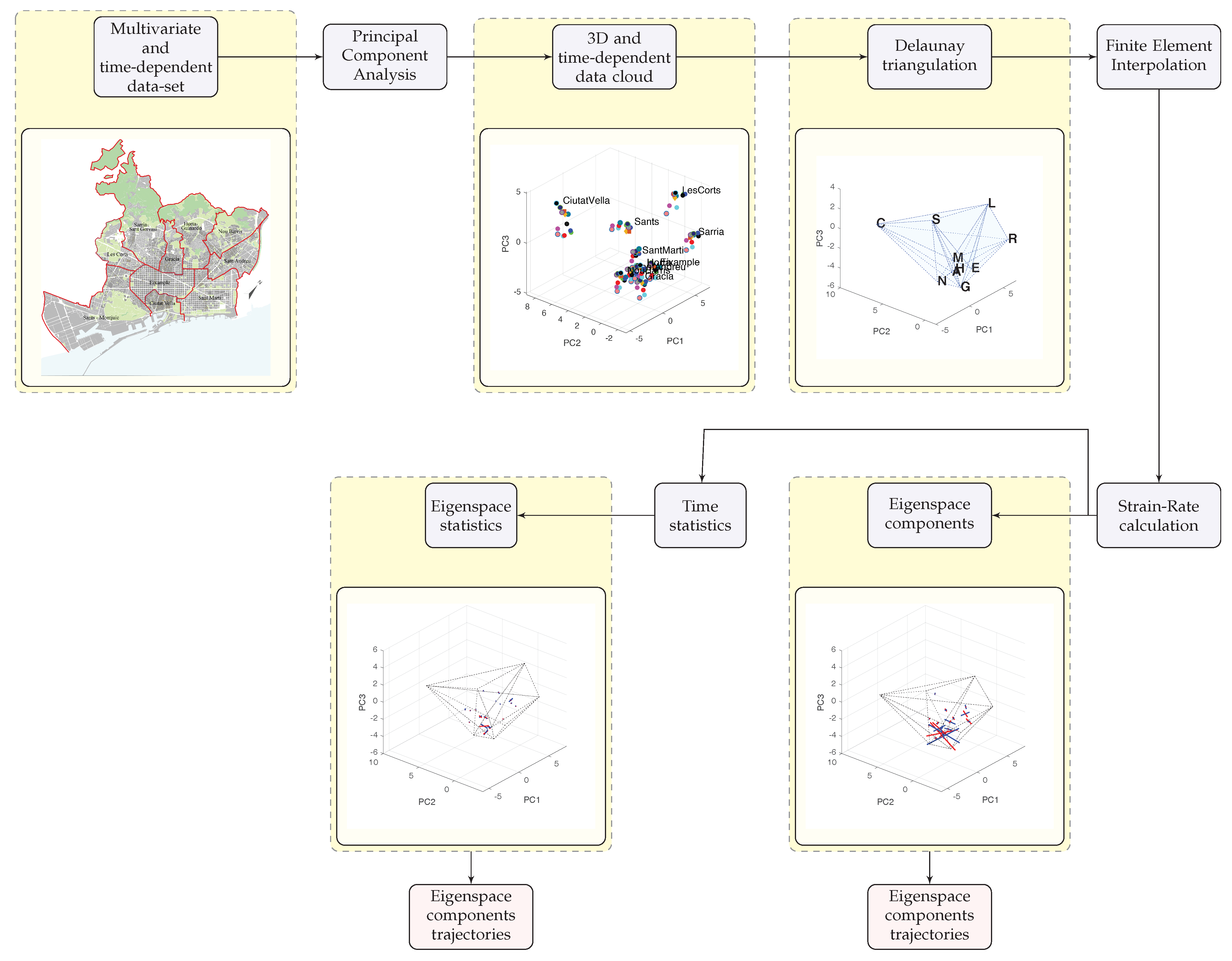
The application of this methodology to the case study is displayed graphically in Figure 4, beginning with the map of the ten districts of Barcelona as the abstraction of the multivariate and time-dependent dataset. The three-dimensional coordinates arising from the PCA output are displayed next. We also present next the triangulated mesh at the initial year 2003. It is clear from the visual inspection that the quantitative analysis of the temporal transformation is greatly justified, thus we calculated the strain-rate tensor over the FEM interpolation of discrete velocities and computed its principal components.

Trajectory Patterns of the Principal Strain-Rates

In favor of the analysis, we display the principal strain-rate components in a graphical way. One approach is to illustrate the patterns of extension-rate and contraction-rate using a vector representation, to what is referred as the strain-rate diagrams [29]. In that approach, the centroid of the tetrahedron serves as the location from which the principal components of the strain-rate tensor give a representative result inside the element. We draw the strain-rate diagram of the year 2003 in the sixth step of Figure 4, where extension-rate is represented by symmetric blue vectors ${\lambda }_1{\mathit{n}}_1$ pointing out the centroid, and contraction-rate is represented by the red vectors ${\lambda }_3{\mathit{n}}_3$ pointing in. However, it is hard to visualize the distribution of the principal strain-rates and their three-dimensional orientations using this type of illustration.

Our approach to ease the visualization and understanding of the strain-rate state is to draw the trajectories of the principal strain-rate components, as used for displaying stresses in beams and columns in [45]. In the following, we demonstrate our findings of the strain-rate state at the year 2003 using the trajectories visualization. In Figure 5, we display the principal components trajectories, where the lines are colored by the magnitude of the principal strain-rate and those are parallel to its orientation. From these representations, we can understand the magnitude and orientation of each principal component of the strain-rate tensor. More importantly, the trajectory patterns overlapped with the coordinates of the districts (in Figure 3) provide information about local regions of extension and contraction rates inside the urban description, where extension-rate patterns indicate differentiation and contraction-rate patterns indicate clustering—or homogenization. This can be observed from the color intensity: locations of high strain-rate are colored with great intensity, while the locations of low deformations are not visible since the white color represents null strain-rates.

In the case of the first strain-rate component, which is shown in Figure 5 (top), we observe that the larger magnitude of extension-rate is localized in the middle of Nou Barris Sant Andreu, Sant Marti, Horta and Sants, and that it decreases near Eixample, Les Corts, and Ciutat Vella. Therefore, the main transformation is located at the group of nearby districts: Nou Barris, Sant Andreu, Sant Marti, and Horta. The extension-rate patterns are oriented from this group apart to Ciutat Vella, suggesting that there is a divergence of Ciutat Vella from the grouped districts. Indeed, the main extension pattern is oriented along the PC3 dimension and covers the grouped districts. The pattern which comprises the districts of Nou Barris, Sant Marti, and Sants and ends at Gracia and Eixample is of lesser importance.

Contraction-rate, on the other hand, is expressed by the third principal strain-rate component, which by definition is orthogonal to the first and second principal strain-rates. The third principal strain-rate component is shown in Figure 5 (bottom), where we can appreciate this orthogonality by noticing that the trajectories of the third principal strain-rate are perpendicular to the extension-rate pattern. We observe that the contraction-rate trajectories are mostly homogeneous, with a minor importance among Sant Marti, Sant Andreu, Nou Barris and Horta districts, and completely declining at Sants and Gracia. This direct relation between extension and contraction is found in solids deformations, where it is ruled by the conservation of mass—or Poisson ratio [23].

Apart from the extension and contraction patterns of the mesh, locations of smaller strain-rates are represented by the second principal component. Considering Figure 5 (middle), we recognize that the orientation of this strain-rate component is concentrated in the middle of Les Corts, Sarria, Horta and Nou Barris, and that it is directed towards Eixample, fading at Ciutat Vella. This principal strain-rate component is certainly orthogonal to the first and second components, but it implies a strain-rate pattern that is two orders of magnitude smaller.

In the previous lines, we have demonstrated the application of the trajectories diagrams of the principal strain-rate components as a powerful visualization technique of the three-dimensional strain-rate state of a data cloud. The strain-rate patterns can be used to analyze the system’s development, for example, with the identification of regions with a special behavior: although there are some grouped districts in the case study, they are all separated at a high rate in the first and third principal components (spatial dimensions). Hence, those are differentiating themselves in the PC1 and PC3 description. On the contrary, low strain-rates can be an indication of stagnation, and, thus, an expression of inactivity where an abrupt change is unlikely to occur. That is especially the case of the Ciutat Vella district, which is separated from the grouped districts but is neither diverging nor converging to them.

One final remark is that our visualization approach is mesh independent. This means that the principal strain-rate trajectory plots coincide regarding the triangulated mesh: different triangulations will produce different positions, magnitudes, and orientations of the principal strain-rate components; nevertheless, the trajectory lines that join them coincide for any type of strain distribution.

3.3. Temporal Statistics of the Principal Strain-Rates

Plots of the principal strain-rate components trajectories can be completed for the remaining years of the time span, $t^n$, $n=1,2,\dots ,11$. Readings of the strain-rate streamline patterns for those years can be completed straightforwardly, as discussed in the paragraphs above. Nevertheless, we performed some temporal statistics of the strain-rate states, where the principal strain-rates calculated for each time-step were considered as the temporal events: each strain-rate state was considered as a single observation.

The first statistics that we performed is the time-average of the principal strain-rate components, separated as the first, second, and third principal strain-rates.

Table 3. Time-averaged eigenspace components.

Element (id)	$\overline{{\mathit{\lambda }}_1}$ (year−1)	$\overline{{\mathit{\lambda }}_2}$ (year−1)	$\overline{{\mathit{\lambda }}_3}$ (year−1)	${\mathit{n}}_1^{\mathbf{\top }}\Rightarrow \overline{{\mathit{\lambda }}_1}$	${\mathit{n}}_2^{\mathbf{\top }}\Rightarrow \overline{{\mathit{\lambda }}_2}$	${\mathit{n}}_3^{\mathbf{\top }}\Rightarrow \overline{{\mathit{\lambda }}_3}$
1	0.1157	−0.0086	−0.0687	[−0.4941 −0.4365 0.7519]	[0.1770 0.1339 −0.9751]	[0.1682 0.8390 0.5175]
2	0.5087	−0.0085	−0.8859	[−0.5777 0.5570 0.5966]	[−0.4259 −0.1592 −0.8907]	[−0.0636 −0.9309 0.3596]
3	0.3919	−0.0440	−0.1662	[−0.3746 −0.7054 0.6017]	[−0.9963 0.0335 0.0789]	[0.3127 −0.7926 −0.5234]
4	0.0868	0.0041	−0.0193	[0.4684 0.8217 0.3247]	[−0.0619 0.3756 −0.9247]	[−0.7437 −0.4144 −0.5246]
5	0.0435	−0.0326	−0.0659	[−0.2319 0.8799 0.4148]	[−0.0891 −0.1728 0.9809]	[0.2229 −0.2816 −0.9333]
6	0.1834	0.0096	−0.0536	[−0.2271 −0.8440 0.4859]	[−0.6281 0.2260 −0.7446]	[−0.4216 0.8544 0.3038]
7	0.0647	−0.0059	−0.0485	[0.5157 −0.6416 0.5678]	[0.0741 −0.9932 0.0893]	[0.2985 −0.4332 −0.8504]
8	0.1436	−0.0198	−0.0174	[−0.3994 −0.4110 0.8194]	[−0.1094 0.9614 −0.2525]	[0.3984 −0.8684 −0.2952]
9	0.6311	0.0178	−0.1144	[−0.2472 −0.6917 0.6785]	[0.2277 0.2955 0.9278]	[0.1771 0.8523 0.4921]
10	0.0355	0.0098	−0.0745	[0.4275 0.8923 −0.1449]	[0.8566 −0.5130 −0.0551]	[−0.5198 0.2220 −0.8249]
11	0.0452	−0.0239	−0.1039	[0.4742 −0.0948 0.8753]	[−0.7018 −0.6930 0.1650]	[−0.3132 −0.9345 −0.1693]
12	0.2054	0.0336	−0.0703	[−0.5086 −0.8385 −0.1954]	[0.1867 0.6566 0.7307]	[0.0460 −0.4726 −0.8801]
13	1.1642	−0.0218	−0.3192	[−0.4080 −0.6299 0.6609]	[−0.9632 0.2605 0.0654]	[−0.5136 0.5798 −0.6325]
14	0.1923	0.0415	−0.2640	[−0.4758 0.8168 0.3264]	[0.9570 0.2693 −0.1076]	[0.4308 −0.2715 −0.8606]
15	0.0552	0.0085	−0.0363	[−0.2364 0.6160 0.7514]	[0.7518 0.2783 −0.5978]	[0.6817 0.6544 −0.3270]
16	0.0438	0.0175	−0.0059	[0.2794 0.9257 −0.2549]	[0.8449 −0.2441 0.4760]	[−0.5430 −0.2892 −0.7883]
17	0.2113	−0.0196	−0.3129	[−0.0062 0.9656 0.2599]	[0.0760 0.2441 0.9668]	[0.0666 −0.9959 −0.0609]

presents the time-averaged results of the principal strain-rates. In addition, in the last schematic of Figure 4, we plot the strain-rate diagram of the time-averaged principal strain-rates at the time-averaged centroid of tetrahedron elements. This figure gives insights about the orientation and magnitude of the first and third principal strain-rates, again by plotting the symmetric arrows pointing out for extension and pointing in for contraction. However, we complete our analysis by drawing the trajectory curves of those time-averaged strain-rate diagrams in Figure 6.

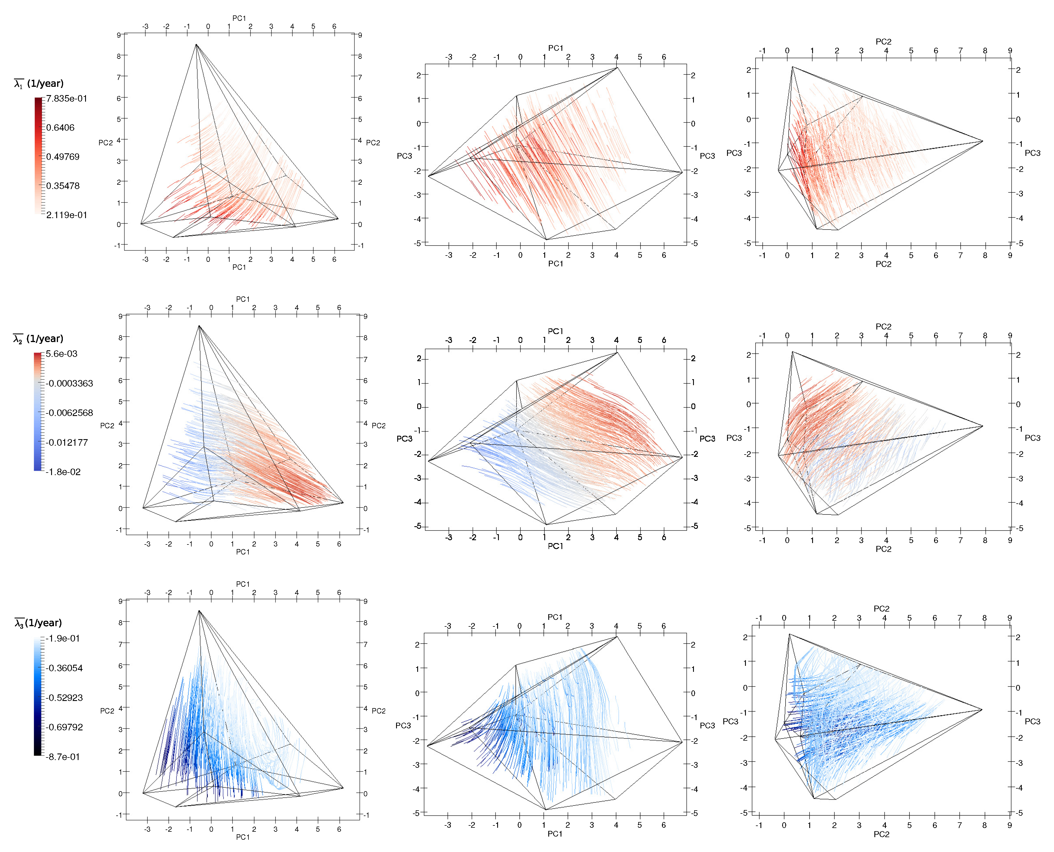
With the aid of Figure 3 and Figure 6, we analyzed the trajectory patterns of the time-averaged strain-rate state of the data cloud. In the case of the first and third strain-rate components, those are comparable to the ones described in the previous paragraphs for the year 2003. We observe a high extension-rate behavior among Nou Barris, Sant Andreu and Horta in the PC1 dimension. The contraction-rate, on the other side, is oriented in the PC2 dimension and it is mostly located in between Gracia and Eixample and decreases near Sants. In the case of the contraction-rate in the PC3 dimension, it is mostly present between Nou Barris and Horta, and in smaller magnitude between Horta and Sant Andreu. The contraction-rate between the remaining districts is negligible in all dimensions. Both the extension and contraction rates demonstrate trajectory patterns that are directed from the grouped districts towards the separated district of Ciutat Vella. However, the magnitude of the time-averaged strain-rates is much smaller than the ones obtained for year 2003. In the case of the time-averaged second strain-rate, its magnitude is greater for Eixample, Les Corts, and Sarria nodes than for the grouped districts. The orientation of the trajectories involving this second strain-rate component is parallel to the one linking Eixample and Les Corts to the grouped districts.

The second temporal statistics we calculated is the $L^{\infty }$-norm of the temporal strain-rate distribution. That is, we calculated the year the maximum extension and contraction rates occurred within each tetrahedron. The results of the application of the $L^{\infty }$-norm to the case study are presented in

Table 4. Maximum and minimum eigenspace components in the time span.

Element(id)	${\mathit{L}}^{\mathbf{\infty }}\left({\mathit{\lambda }}_1\right)$	Year	${\mathit{n}}_1^{\mathbf{\top }}\Rightarrow {\mathit{L}}^{\mathbf{\infty }}\left({\mathit{\lambda }}_1\right)$	${\mathit{L}}^{-\mathbf{\infty }}\left({\mathit{\lambda }}_3\right)$	Year	${\mathit{n}}_3^{\mathbf{\top }}\Rightarrow {\mathit{L}}^{-\mathbf{\infty }}\left({\mathit{\lambda }}_3\right)$
1	0.5315	2003	[−0.4030 −0.7620 0.5069]	−0.5035	2003	[0.3339 −0.6381 −0.6938]
2	2.0893	2010	[−0.5094 0.8338 0.2130]	−3.2621	2003	[0.0250 0.8977 −0.4399]
3	3.0249	2009	[−0.0766 −0.8956 0.4383]	−1.2631	2003	[−0.4015 0.6447 0.6505]
4	0.4860	2010	[0.5309 0.8024 0.2724]	−0.1901	2005	[0.8017 0.5583 −0.2134]
5	0.6321	2014	[0.0691 0.9893 −0.1286]	−0.3019	2010	[−0.3219 0.5283 0.7857]
6	1.1842	2006	[0.1651 −0.9360 0.3110]	−0.9833	2005	[0.2453 −0.7335 −0.6338]
7	0.2772	2010	[0.0108 −0.9360 0.3518]	−0.2122	2003	[0.1777 −0.2093 0.9616]
8	0.5104	2010	[−0.4614 −0.6584 0.5946]	−0.5374	2009	[−0.2484 −0.6025 0.7585]
9	4.3858	2010	[−0.2509 −0.6991 0.6696]	-2.4530	2010	[0.4203 −0.7018 −0.5752]
10	0.3753	2010	[−0.4800 0.8570 −0.1874]	−0.3477	2009	[0.4401 −0.6943 0.5695]
11	0.5210	2009	[−0.0542 0.3205 0.9457]	−0.5164	2009	[0.3738 0.8847 −0.2784]
12	1.5272	2008	[−0.6804 −0.7328 0.0027]	−0.7379	2007	[0.4304 0.8624 −0.2666]
13	5.2538	2003	[−0.2599 −0.7733 0.5783]	−4.6094	2008	[0.2022 −0.9445 0.2588]
14	2.5830	2003	[−0.4920 0.6994 0.5184]	−2.0295	2003	[−0.3863 −0.7091 0.5900]
15	0.2810	2003	[−0.6611 −0.5949 0.4572]	−0.4221	2010	[0.0927 −0.9519 −0.2919]
16	0.2659	2009	[0.4571 0.7618 −0.4591]	−0.1636	2012	[−0.5501 0.7352 0.3961]
17	1.4269	2009	[−0.0935 0.9952 0.0288]	−1.1715	2010	[0.1262 0.9888 0.0798]

. We observe that the maximum strain-rates occurred in year 2003: either expansion or contraction. In addition, the important contraction-rate magnitudes took place between the years 2003 and 2010. This is not the case of the extension-rate magnitudes, which are more prevalent after year 2008.

4. Conclusions

In this study, we quantified the temporal change of a time-dependent and three-dimensional dataset. Contrary to other approaches [1,7,11,14], we calculated the three-dimensional strain-rate state of the dataset based on the interpolation of discrete point-wise displacements—or data variations. We applied a technique in continuum mechanics using a FEM interpolation of non-overlapping linear tetrahedral elements that covers the three-dimensional dataset.

The methodology was demonstrated to exhibit regions of major deformation-rate. Departing from the calculation of the numerical strain-rate values, we introduced some data-visualization techniques that help to locate the magnitudes and orientations of the strain-rate state in the three-dimensional framework. This was the case of the principal strain-rate trajectories, which where demonstrated to be more detailed than other possible visualization techniques, e.g., strain-rate diagrams [32,36] or confidence ellipsoids [18,19,20,21,22]. The main difference with strain-rate diagrams is the ability of the present approach to display a continuum version of the strain-rate inside the dataset, and to separate the analysis into each principal component of the strain-rate state, while being mesh independent. Compared to the method of confidence ellipsoids, the kinematic basis of the proposed methodology makes an accurate description of the deformation patterns in the complete three-dimensional domain, rather than in a compact and partial region that contains the data distribution. It also allows a detailed temporal description of the change between one instant and another. This is specifically not possible using the method of the ellipsoids since that method accounts for the complete temporal distribution in order to evaluate change.

The calculation of the strain-rate state shows that the methodology is suitable for quantifying the temporal change of a reduced three-dimensional dataset describing the social, economic and environmental state of the city of Barcelona. In particular, high strain-rates are associated with the localized deformation of regions that represent the districts of the city in the time span of 13 years. The method not only portrays the similarities and differences—distances—between the districts of the city, similar to cluster analysis [46,47,48] or distance measures [49,50], which explore similarities and groups in data. The distinctive attribute of the present work is the feasibility to quantify the districts’ differentiation with time: the strain-rate tensor provides quantitative information about local regions of extension and contraction, where extension-rate patterns indicate differentiation and contraction-rate patterns indicate clustering—or homogenization. In this regard, the strain-rate methodology can be potentially used as an extension of clustering analysis, since it reveals contraction and extension patterns of clusters. Conclusions about the divergence or clustering of districts in time can therefore be stated. For example, it reveals the time, location, and orientation of pressures affecting the inhabitants of certain districts of the city, essentially those which are rapidly diverging from the rest (e.g., the case of Ciutat Vella for the case study). This methodology locates regions where detailed action is necessary, as well as the foretelling of possible ruptures in the system.

Finally, we mention that this method is not limited to the study of the data change, but can also be applied to other descriptions: a natural sequel to the present article is the study of the time-dependent data cloud as a deforming elastic solid under equilibrium. Solving the inverse problem, namely the identification of the constitutive moduli of the deforming material, emerges as the first step for predicting the system’s future state given its historical data.

References

- Fuchs, R.; Hauser, H. Visualization of multi-variate scientific data. In Computer Graphics Forum; Blackwell Publishing Ltd.: Oxford, UK, 2009; Volume 28, pp. 1670–1690. [Google Scholar]
- Salazar-Llano, L.; Rosas-Casals, M.; Ortego, M.I. An Exploratory Multivariate Statistical Analysis to Assess Urban Diversity. Sustainability 2019, 11, 3812. [Google Scholar] [CrossRef]
- White, F.M.; Corfield, I. Viscous Fluid Flow; McGraw-Hill: New York, NY, USA, 2006; Volume 3. [Google Scholar]
- Bower, A.F. Applied Mechanics of Solids; CRC Press: Boca Raton, FL, USA, 2009. [Google Scholar]
- McLoughlin, T.; Laramee, R.S.; Peikert, R.; Post, F.H.; Chen, M. Over two decades of integration-based, geometric flow visualization. In Computer Graphics Forum; Blackwell Publishing Ltd.: Oxford, UK, 2010; Volume 29, pp. 1807–1829. [Google Scholar]
- Süßmuth, J.; Winter, M.; Greiner, G. Reconstructing animated meshes from time-varying point clouds. In Computer Graphics Forum; Blackwell Publishing Ltd.: Oxford, UK, 2008; Volume 27, pp. 1469–1476. [Google Scholar]
- Ustinin, M.N.; Kronberg, E.; Filippov, S.V.; Sytchev, V.V.; Sobolev, E.V.; Llinás, R. Kinematic visualization of human magnetic encephalography. Math. Biol. Bioinform. 2010, 5, 176–187. [Google Scholar]
- Wang, S.W.; Interrante, V.; Longmire, E. Multivariate visualization of 3D turbulent flow data. In Proceedings of the Visualization and Data Analysis 2010, San Jose, CA, USA, 17–21 January 2010; International Society for Optics and Photonics: Bellingham, WA, USA, 2010; Volume 7530, p. 75300N. [Google Scholar]
- Kohler, M.; Krzyżak, A. Nonparametric estimation of non-stationary velocity fields from 3D particle tracking velocimetry data. Comput. Stat. Data Anal. 2012, 56, 1566–1580. [Google Scholar] [CrossRef]
- Aguirre-Pablo, A.; Aljedaani, A.B.; Xiong, J.; Idoughi, R.; Heidrich, W.; Thoroddsen, S.T. Single-camera 3D PTV using particle intensities and structured light. Exp. Fluids 2019, 60, 25. [Google Scholar] [CrossRef] [Green Version]
- Keim, D.A. Information visualization and visual data mining. IEEE trans. Vis. Comput. Graphics 2002, 8, 1–8. [Google Scholar] [CrossRef]
- Gao, L.; Heath, D.G.; Kuszyk, B.S.; Fishman, E.K. Automatic liver segmentation technique for three-dimensional visualization of CT data. Radiology 1996, 201, 359–364. [Google Scholar] [CrossRef] [PubMed]
- Teplan, M. Fundamentals of EEG measurement. Meas. Sci. Rev. 2002, 2, 1–11. [Google Scholar]
- Wang, C.; Yu, H.; Ma, K.L. Importance-driven time-varying data visualization. IEEE Trans. Vis. Comput. Graphics 2008, 14, 1547–1554. [Google Scholar] [CrossRef]
- Husson, F.; Lê, S.; Pagès, J. Confidence ellipse for the sensory profiles obtained by principal component analysis. Food Quality Prefer. 2005, 16, 245–250. [Google Scholar] [CrossRef]
- Cadoret, M.; Husson, F. Construction and evaluation of confidence ellipses applied at sensory data. Food Quality Prefer. 2013, 28, 106–115. [Google Scholar] [CrossRef]
- Abdi, H.; Williams, L.J.; Valentin, D. Multiple factor analysis: principal component analysis for multitable and multiblock data sets. Wiley Int. Rev. Comput. Stat. 2013, 5, 149–179. [Google Scholar] [CrossRef]
- Werth, M.T.; Halouska, S.; Shortridge, M.D.; Zhang, B.; Powers, R. Analysis of metabolomic PCA data using tree diagrams. Anal. Biochem. 2010, 399, 58–63. [Google Scholar] [CrossRef] [PubMed] [Green Version]
- Worley, B.; Halouska, S.; Powers, R. Utilities for quantifying separation in PCA/PLS-DA scores plots. Anal. Biochem. 2013, 433, 102–104. [Google Scholar] [CrossRef] [PubMed]
- Wang, B.; Shi, W.; Miao, Z. Confidence analysis of standard deviational ellipse and its extension into higher dimensional Euclidean space. PLoS ONE 2015, 10, e0118537. [Google Scholar] [CrossRef] [PubMed]
- Josse, J.; Wager, S.; Husson, F. Confidence areas for fixed-effects pca. J. Comput. Graph. Stat. 2016, 25, 28–48. [Google Scholar] [CrossRef]
- Cederholm, P. Deformation analysis using confidence ellipsoids. Surv. Rev. 2003, 37, 31–45. [Google Scholar] [CrossRef]
- Mase, G.T.; Smelser, R.E.; Mase, G.E. Continuum Mechanics for Engineers; CRC Press: Boca Raton, FL, USA, 2009. [Google Scholar]
- Marsden, J.E.; Hughes, T.J. Mathematical Foundations of Elasticity; Courier Corporation: North Chelmsford, MA, USA, 1994. [Google Scholar]
- Xu, P.; Grafarend, E. Statistics and geometry of the eigenspectra of three-dimensional second-rank symmetric random tensors. Geophys. J. Int. 1996, 127, 744–756. [Google Scholar] [CrossRef]
- Wdowinski, S.; Sudman, Y.; Bock, Y. Geodetic detection of active faults in S. California. Geophys. Res. Lett. 2001, 28, 2321–2324. [Google Scholar] [CrossRef] [Green Version]
- Straub, C.; Kahle, H.G.; Schindler, C. GPS and geologic estimates of the tectonic activity in the Marmara Sea region, NW Anatolia. J. Geophys. Res. Solid Earth 1997, 102, 27587–27601. [Google Scholar] [CrossRef]
- Moin, P. Fundamentals of Engineering Numerical Analysis; Cambridge University Press: Cambridge, UK, 2010. [Google Scholar]
- Hackl, M.; Malservisi, R.; Wdowinski, S. Strain rate patterns from dense GPS networks. Nat. Hazards Earth Syst. Sci. 2009, 9, 1177–1187. [Google Scholar] [CrossRef] [Green Version]
- Wang, H.; Amini, A.A. Cardiac motion and deformation recovery from MRI: A review. IEEE Trans. Med Imaging 2012, 31, 487–503. [Google Scholar] [CrossRef] [PubMed]
- Pedrizzetti, G.; Sengupta, S.; Caracciolo, G.; Park, C.S.; Amaki, M.; Goliasch, G.; Narula, J.; Sengupta, P.P. Three-dimensional principal strain analysis for characterizing subclinical changes in left ventricular function. J. Am. Soc. Echocardiogr. 2014, 27, 1041–1050. [Google Scholar] [CrossRef] [PubMed]
- Cai, J.; Grafarend, E.W. Statistical analysis of geodetic deformation (strain rate) derived from the space geodetic measurements of BIFROST Project in Fennoscandia. J. Geodyn. 2007, 43, 214–238. [Google Scholar] [CrossRef]
- Cai, J.; Grafarend, E.W. Statistical analysis of the eigenspace components of the two-dimensional, symmetric rank-two strain rate tensor derived from the space geodetic measurements (ITRF92-ITRF2000 data sets) in central Mediterranean and Western Europe. Geophys. J. Int. 2007, 168, 449–472. [Google Scholar] [CrossRef] [Green Version]
- Mastrolembo, B.; Caporali, A. Stress and strain-rate fields: A comparative analysis for the Italian territory. Bollettino di Geofisica Teorica ed Applicata 2017, 58, 265–284. [Google Scholar]
- Houlie, N.; Woessner, J.; Giardini, D.; Rothacher, M. Lithosphere strain rate and stress field orientations near the Alpine arc in Switzerland. Sci. Rep. 2018, 8, 2018. [Google Scholar] [CrossRef] [Green Version]
- Su, X.; Yao, L.; Wu, W.; Meng, G.; Su, L.; Xiong, R.; Hong, S. Crustal deformation on the northeastern margin of the Tibetan plateau from continuous GPS observations. Remote Sens. 2019, 11, 34. [Google Scholar] [CrossRef]
- Sneddon, I.N. The distribution of stress in the neighbourhood of a crack in an elastic solid. Proc. R. Soc. Lond. Ser. Math. Phys. Sci. 1946, 187, 229–260. [Google Scholar]
- Williams, M. The bending stress distribution at the base of a stationary crack. Trans. ASME 1957, 79, 109–114. [Google Scholar] [CrossRef]
- Aktuğ, B.; Parmaksız, E.; Kurt, M.; Lenk, O.; Kılıçoğlu, A.; Gürdal, M.A.; Özdemir, S. Deformation of central anatolia: GPS implications. J. Geodyn. 2013, 67, 78–96. [Google Scholar] [CrossRef]
- Grafarend, E. Criterion matrices for deforming networks. In Optimization and Design of Geodetic Networks; Springer: Berlin/Heidelberg, Germany, 1985; pp. 363–428. [Google Scholar]
- Grafarend, E.W. Three-dimensional deformation analysis: Global vector spherical harmonic and local finite element representation. Tectonophysics 1986, 130, 337–359. [Google Scholar] [CrossRef]
- Dermanis, A.; Grafarend, E. The finite element approach to the geodetic computation of two-and three-dimensional deformation parameters: A study of frame invariance and parameter estimability. In Proceedings of the International Conference “Cartography-Geodesy”, Maracaibo, Venezuela, 24 November–3 December 1992. [Google Scholar]
- De Berg, M.; Van Kreveld, M.; Overmars, M.; Schwarzkopf, O. Computational geometry. In Computational Geometry; Springer: Berlin/Heidelberg, Germany, 1997; pp. 1–17. [Google Scholar]
- Marot, C.; Pellerin, J.; Remacle, J.F. One machine, one minute, three billion tetrahedra. Int. J. Numer. Methods Eng. 2019, 117, 967–990. [Google Scholar] [CrossRef]
- Gere, J.M.; Goodno, B.J. Mechanics of Materials, Brief Edition; Cengage Learning: Boston, MA, USA, 2012. [Google Scholar]
- Clemants, S.; Moore, G. Patterns of Species Diversity in Eight Northeastern United States Cities; Urban Habitats: Goodwood, Australia, 2003; Volume 1. [Google Scholar]
- Raudsepp-Hearne, C.; Peterson, G.D.; Bennett, E.M. Ecosystem service bundles for analyzing tradeoffs in diverse landscapes. Proc. Natl. Acad. Sci. USA 2010, 107, 5242–5247. [Google Scholar] [CrossRef] [PubMed] [Green Version]
- Kaufman, L.; Rousseeuw, P.J. Finding Groups in Data: An Introduction to Cluster Analysis; John Wiley & Sons: Hoboken, NJ, USA, 2009; Volume 344. [Google Scholar]
- Laliberté, E.; Legendre, P. A distance-based framework for measuring functional diversity from multiple traits. Ecology 2010, 91, 299–305. [Google Scholar] [CrossRef]
- Cha, S.H. Comprehensive survey on distance/similarity measures between probability density functions. City 2007, 1, 1. [Google Scholar]
Figure 1.
Flow chart of the visualization methodology.
Figure 2.
Three-dimensional and time-dependent data cloud from the case study.
Figure 3.
Delaunay triangulation of the data cloud from the case study.
Figure 4.
Flow chart of the temporal change visualization methodology.
Figure 5.
The trajectory patterns of the principal strain-rates at the year 2003: first principal strain-rate (top); second principal strain-rate (middle); and third principal strain-rate (bottom). The color scale in these graphs determines the strain type: the red color is used to represent extension, while the blue color depicts contraction.
Figure 6.
The trajectory patterns of the time-averaged principal strain-rates: averaged first principal strain-rate (top); averaged second principal strain-rate (middle); and averaged third principal strain-rate (bottom). In these graphs, the red color is used to represent extension, while the blue color depicts contraction.