A Comparative Study of Continuum and Structural Modelling Approaches to Simulate Bone Adaptation in the Pelvic Construct


1
The Royal British Legion Centre for Blast Injury Studies, Imperial College London, London SW7 2AZ, UK
2
Department of Civil and Environmental Engineering, Structural Biomechanics, Imperial College London, London SW7 2AZ, UK
*
Author to whom correspondence should be addressed.
Appl. Sci. 2019, 9(16), 3320; https://doi.org/10.3390/app9163320
Submission received: 27 June 2019
/
Revised: 29 July 2019
/
Accepted: 7 August 2019
/
Published: 13 August 2019
(This article belongs to the Special Issue Biomaterials for Bone Tissue Engineering)
Abstract
:This study presents the development of a number of finite element (FE) models of the pelvis using different continuum and structural modelling approaches. Four FE models were developed using different modelling approaches: continuum isotropic, continuum orthotropic, hybrid isotropic and hybrid orthotropic. The models were subjected to an iterative adaptation process based on the Mechanostat principle. Each model was adapted to a number of common daily living activities (walking, stair ascent, stair descent, sit-to-stand and stand-to-sit) by applying onto it joint and muscle loads derived using a musculoskeletal modelling framework. The resulting models, along with a structural model previously developed by the authors, were compared visually in terms of bone architecture, and their response to a single load case was compared to a continuum FE model derived from computed tomography (CT) imaging data. The main findings of this study were that the continuum orthotropic model was the closest to the CT derived model in terms of load response albeit having less total bone volume, suggesting that the role of material directionality in influencing the maximum orthotropic Young’s modulus should be included in continuum bone adaptation models. In addition, the hybrid models, where trabecular and cortical bone were distinguished, had similar outcomes, suggesting that the approach to modelling trabecular bone is less influential when the cortex is modelled separately.
1. Introduction
The pelvic construct is the region of load transition between the upper body and lower limbs and plays a number of roles, such as protecting the organs and vessels in the lower abdomen. It also facilitates the transfer of forces between the lower limbs and the upper body during physical activities such as walking and stair climbing, withstanding loads at the hip joints of up to around six times body weight [1,2,3].
Continuous adaptation of bone tissue in response to the mechanical environment surrounding it provides an explanation for the different architecture of bones in the skeletal system [4]. Long bones, such as the femur and tibia, develop thick cortical shafts with trabecular bone concentrated at the joints to transfer contact forces [5,6], whereas the pelvis is viewed as a sandwich structure where a thin layer of cortical bone surrounds a structure of trabecular bone [7,8,9].
Finite element (FE) modelling is a very common approach to investigate the biomechanics of the pelvic ring due to its versatility and low cost compared to clinical investigations, with the added characteristic of enabling the design of bone scaffolds or implants. Computational modelling of bone adaptation to the mechanical environment surrounding it has emerged into an important component in aiding the interpretation of experimental findings and exploring further issues [10,11]. Bone adaptation models have been previously developed using both continuum elements [12,13,14,15] or structural elements [6,16,17,18]. Early FE models either used simplified geometries [19,20,21,22], were axisymmetric [23,24] or reduced the three-dimensional pelvis to a two-dimensional slice [25,26,27,28,29].
The first FE model of the bony pelvis based on subject specific geometry and material properties from medical imaging data was developed by Dalstra et al. [30] using continuum solid elements, validating it against experimentally obtained data from a cadaveric pelvis loaded at the hip joint. Anderson et al. [9] developed an FE model of the pelvic innominate by distinguishing between cortical and trabecular bone using different element types. Cortical bone was modelled using structural shell elements with location dependent thickness derived from medical imaging data. Trabecular bone was modelled using continuum isotropic elements and the model was validated against experimental data by comparing cortical bone strains. The majority of recent FE models representing the pelvic construct were developed from CT imaging data with a tendency of using an isotropic material model to represent bone and distinguishing between trabecular and cortical bone by adding a layer of shell elements [9,31,32]. Notably, Anderson et al. [9] also developed a purely continuum model in which the surface nodes were assigned the highest Young’s modulus they found for cancellous bone (approximately 3.8 GPa) which performed similarly to the model with a shell element layer. Although modelling bone using isotropic material properties has the benefit of reducing computational time, it is insufficient to provide information on directionality of the bone microstructure [33]. Orthotropy has been found to offer a good approximation of bone’s anisotropy at the continuum level [34].
The aim of this study was to develop a number of computational models of the pelvic construct using different continuum and structural FE bone adaptation modelling approaches with the purpose of investigating their effects on bone adaptation and predicted mechanical behaviour of the pelvis in comparison to a CT scan derived FE model. The modelling approaches were divided into isotropic and orthotropic material models, followed by a continuum or hybrid approach, where cortical and trabecular bone were distinguished. The motivation behind developing a number of different models was to assess their sensitivity to the approach used. Each model was subjected to an iterative adaptation algorithm based on the Mechanostat principle [4] and tailored for the type of elements used [6,14]. Bone adaptation was driven by the strains generated by a loading environment derived from five daily living activities (walking, stair ascent, stair descent, sit-to-stand and stand-to-sit).
2. Methods
2.1. Musculoskeletal Modelling
To obtain a physiologically relevant morphological representation of the pelvic construct, the base FE models were subjected to a loading environment derived from musculoskeletal simulations of the five most frequent daily living activities [35]: walking, stair ascent, stair descent, sit-to-stand and stand-to-sit. The simulations were performed using a bilateral musculoskeletal model of the lower limbs. The model was based on an ipsilateral model developed by Modenese et al. [36] based on an anatomical dataset published by Horsman et al. [37] and implemented in OpenSim [38]. The model was validated at the hip joint. The bilateral model had a total of 76 muscles and 326 actuators. Further details can be found in Zaharie and Phillips [39].
Gait data for the selected physical activities were collected from a male volunteer (age: 23 years, weight: 93 kg, height: 188 cm) at the Human Biodynamics Lab in the Imperial College Research Labs at Charing Cross Hospital and processed using Vicon Nexus and the Biomechanical ToolKit [40]. A total of 59 reflective markers were positioned on bony landmarks and tracked using a Vicon system (Oxford Metrics, Oxford, UK) equipped with 10 infrared cameras. Ground reaction forces (GRFs) were measured using three force plates (Type 9286BA, sampling rate 1000 Hz, Kistler Instruments Ltd, Hook, UK). For walking, the force plates were placed to form a walkway (speed: 1.34 m/s, stride length: 0.64 m, cadence: 115.54 steps/min). A staircase was instrumented with the force plates to record stair ascent and stair descent GRFs (step height 15 cm and step depth 25 cm). Three force plates were set, one under each foot and another on a stool with a height of 52.5 cm from the floor to measure ground and seat reaction forces during sit-to-stand and stand-to-sit.
The body segments of the model were scaled to the anatomical dimensions of the volunteer by calculating the ratios between the lengths given by experimental and virtual markers. The inertial properties of each segment were updated using the regression equations of Dumas et al. [41]. The joint angles for each recorded activity were derived using an inverse kinematic approach [42]. Static optimization with a cost function minimising the sum of muscle activations squared was performed to estimate the muscle forces throughout each activity’s cycle. The muscle insertion points on the pelvis along with the direction and magnitude of each muscle force were extracted using the MuscleForceDirection (v1.0) plugin [6,43]. The hip joint contact forces were calculated using the JointReaction tool available in OpenSim [44]. The musculoskeletal modelling was performed using OpenSim (Version 3.3) [38]. The loads applied on the pelvis throughout the duration of each activity cycle (hip joint reaction forces, muscle forces and inertial forces) were determined and subsampled to maintain computational efficiency, resulting in a total of 39 load cases representing the five physical activities.
2.2. Finite Element Modelling
2.2.1. Base Model
The base FE model used in this study was generated from a tetrahedral mesh previously developed by the authors [39]. The volumetric mesh of the pelvis was generated in Mimics (Materialise, Leuven, Belgium) from a CT scan (399 × 3 mm thick slices, 512 × 512 pixels, 0.91 mm/pixel) of a cadaveric pelvis and lower limbs (Male, age: 55, weight: 94.3 kg, height: 188 cm) provided by the Royal British Legion Centre for Blast Injury Studies at Imperial College London, to which the volunteer was height and weight matched. The base FE model consisted of 377,362 tetrahedral elements with an average edge length of 3.76 mm [39]. In the present study, four predictive models of the pelvic construct were developed: two purely continuum models with orthotropic and isotropic material properties, and two hybrid models where trabecular and cortical bone were differentiated using continuum and shell elements respectively, while assigning orthotropic and isotropic material properties to elements representing trabecular bone (Table 1). In addition, a structural model previously developed by the authors [39] was included for comparison.
2.2.2. Ligaments
To realistically model the load transfer between the three pelvic bones, the ligaments associated with the pelvic ring (sacro-iliac, pubic, sacrospinous, sacrotuberous and inguinal) were included in the model. The anatomical attachment areas of each ligament were visually defined on the model based on descriptions in the literature [45,46,47,48].
Each ligament was modelled using truss elements between each pair of closest nodes from the two surfaces corresponding to the insertions areas. All truss elements representing ligaments were assigned linear elastic material properties and zero stiffness in compression. A set of truss elements with a low compressive Young’s modulus was overlaid with the initial truss elements for each ligament to ensure numerical stability. For the joints containing cartilage, truss elements were included to allow the transfer of compressive forces. The tensile and compressive material properties assigned to the ligaments and cartilage were taken from a previous study [39].
2.2.3. Loading and Boundary Conditions
The 39 load cases resulting from the musculoskeletal simulations were applied on the model in successive analysis steps. The muscle forces obtained from the musculoskeletal model were applied as point loads on the closest three nodes to each muscle insertion point [39,49]. The hip joint contact forces and the inertial loads were applied at the joint centres and the centre of mass of the pelvic segment, respectively. In addition, for sit to stand and stand to sit, the reaction load from the seat was applied at the inferior ischium for the duration of contact. To spread the hip joint contact forces over the corresponding bone surface, they were applied using `load applicators’ comprising of four layers of continuum wedge elements, each with a thickness of 2 mm, as they allow for a reduction in CPU time in comparison to modeling contact at each joint. The two first layers were assigned material properties akin to cartilage (E = 10 MPa, = 0.49), with the furthest two being assigned stiffnesses of 10 MPa ( = 0.3) and 500 MPa ( = 0.3), respectively [6,39]. In addition, an `inertial applicator’ was designed to spread the inertial load of the pelvis over the whole construct by linking its centre of mass to every node of the model with truss elements with a radius of 0.1 mm and low stiffness (E = 0.1 MPa, = 0.3) to avoid artificially stiffening the model. The L5S1 interface between the lumbar spine and the sacrum was constrained in the three translational degrees of freedom via four layers of wedge elements to avoid fixing nodes directly on the bone surface resulting in artificial stress concentrations. The layers were respectively assigned the same thickness and material properties as the load applicators.
The load cases obtained from the musculoskeletal model were applied in consecutive analysis steps to the FE model.
2.3. Bone Adaptation
The base FE models were subjected iteratively to the aforementioned load cases using an adaptation algorithm based on the Mechanostat principle [4] proposed by Geraldes and Phillips [14] for the continuum orthotropic and isotropic elements used in the continuum and hybrid models. After each iteration, the material properties of each orthotropic element were adjusted depending on the stresses and strains occuring due to the applied loading regime. A guiding step was selected for each element based on the absolute maximum principal strain value from all analysis steps. The stress tensor associated with that step was then used to extract the principal stresses and their orientation by performing an eigenanalysis.
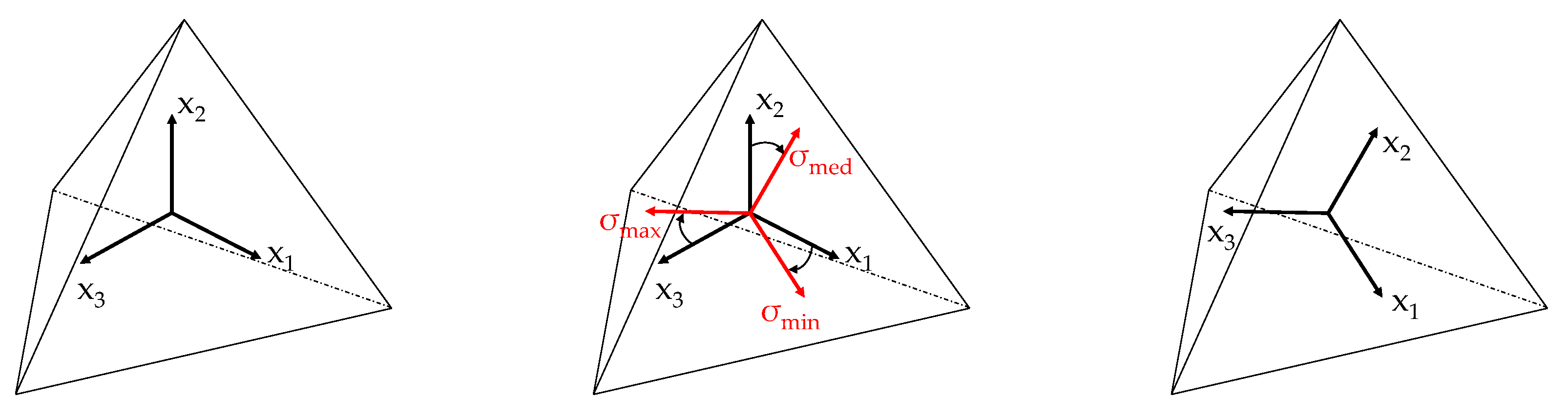
The axes representing the orthotropic orientations of each element were aligned to the vectors defining the principal stress directions for the guiding frame (Figure 1).
Young’s moduli and shear moduli were updated proportional to the absolute maximum normal and shear strains for the orientation obtained from the guiding step across all analysis steps, compared to the normal strain target and shear strain target, respectively. Poisson’s ratios for each element were altered to satisfy the thermodynamic restrictions on the elastic constant of bone and maintain the compliance matrix as positive definite [15].
For the isotropic elements, the Young’s modulus of each element was updated proportionally to the absolute maximum principal strain taken across all loading frames, while Poisson’s ratio was kept constant. Concerning the hybrid models, shell elements representing cortical bone were adjusted in a similar fashion by modifying their thickness according to the in-plane absolute maximum strain as implemented in previous work from the research group [6,39,50].
To satisfy the Mechanostat principle [4], material and geometric properties of the elements were adjusted to bring the local normal strains towards a target strain, assigned a value of 1250 . The lazy zone interval was defined between 1000 and 1500 . In the case of models with orthotropic elements, the shear target strain was assigned a value of 1443 with a lazy zone of 1154 and 1732 , in concordance with previous studies from the research group [6,14,15]. In addition, normal strains lower than 250 were associated with the dead zone.
The elements of the continuum models were assigned an initial Young’s modulus value of 3000 MPa and a Poisson’s ratio of 0.3. In addition, for the continuum orthotropic model, the initial values of shear modulus were set at 1500 MPa. The Young’s modulus values were limited between 10 and 18,000 MPa [30]. The limits of shear modulus values for continuum orthotropic model were set between 5 and 15000 MPa. Elements with strains in the dead zone were assigned the minimum allowable Young’s modulus and were not re-adjusted in subsequent iterations of the the adaptation process. The convergence criterion was defined as when the average change in Young’s moduli of elements with absolute normal strain values above 250 and Young’s moduli above the minimum was less than 2% between successive iterations [13].
In the case of the hybrid models, a distinction was made between cortical and trabecular bone. Continuum elements, representing trabecular bone, were assigned initial Young’s modulus values of 300 MPa, limited between 10 and 2000 MPa and Possion’s ratio values of 0.3 [30]. For the hybrid orthotropic model, elements were assigned initial shear modulus values of 150 MPa, limited between 5 and 1500 MPa. Each shell element, representative of cortical bone, was assigned a Young’s modulus of 18,000 MPa, a Poisson’s ratio of 0.3 and an initial thickness of 0.1 mm [6]. Cortical thickness was limited between 0.1 mm and 5 mm [39]. The thickness of cortical elements was updated proportional to the largest value of maximum principal strain across all load cases and the target normal strain. The convergence criterion for shell elements adaptation was defined as when less than 1% of shell elements changed their thickness between successive iterations [6]. Convergence of the hybrid models was achieved only when both structural and continuum convergence criteria were met simultaneously.
A structural model of the pelvis developed previously [39] was included in the comparison. Briefly, the structural model was developed using a network of truss elements to represent trabecular bone and shell elements to represent cortical bone. The thickness of shells and cross-sectional area of trusses were updated proportional to absolute maximum principal strains resulting from the same set of load cases used in this study and the same target normal strain. Similarly, convergence was achieved when less than 2% of elements changed their thickness or cross-sectional area between successive iterations.
2.4. Comparison with CT Scan Derived Model
The tetrahedral mesh of the right hemipelvis was assigned varying material properties derived from the CT scan data (Figure 2) using Bonemat [51]. Assuming a linear relationship between the Hounsfield units (HU) values in the scans and bone ash density [52], bone ash density distribution was derived from the medical images. Young’s moduli (GPa) for each element were derived from the ash density (g/cm3) using a power relationship [53]. This model was not used in the adaptation and was developed to provide an independent comparison for the adaptive models. The response of the resulting CT derived FE model and the corresponding adapted models to a vertical load of 2 kN applied at the acetabulum representing a standing stance were compared. The hemipelvis was constrained at the pubic and sacroiliac joint surfaces.
3. Results
3.1. Continuum Models
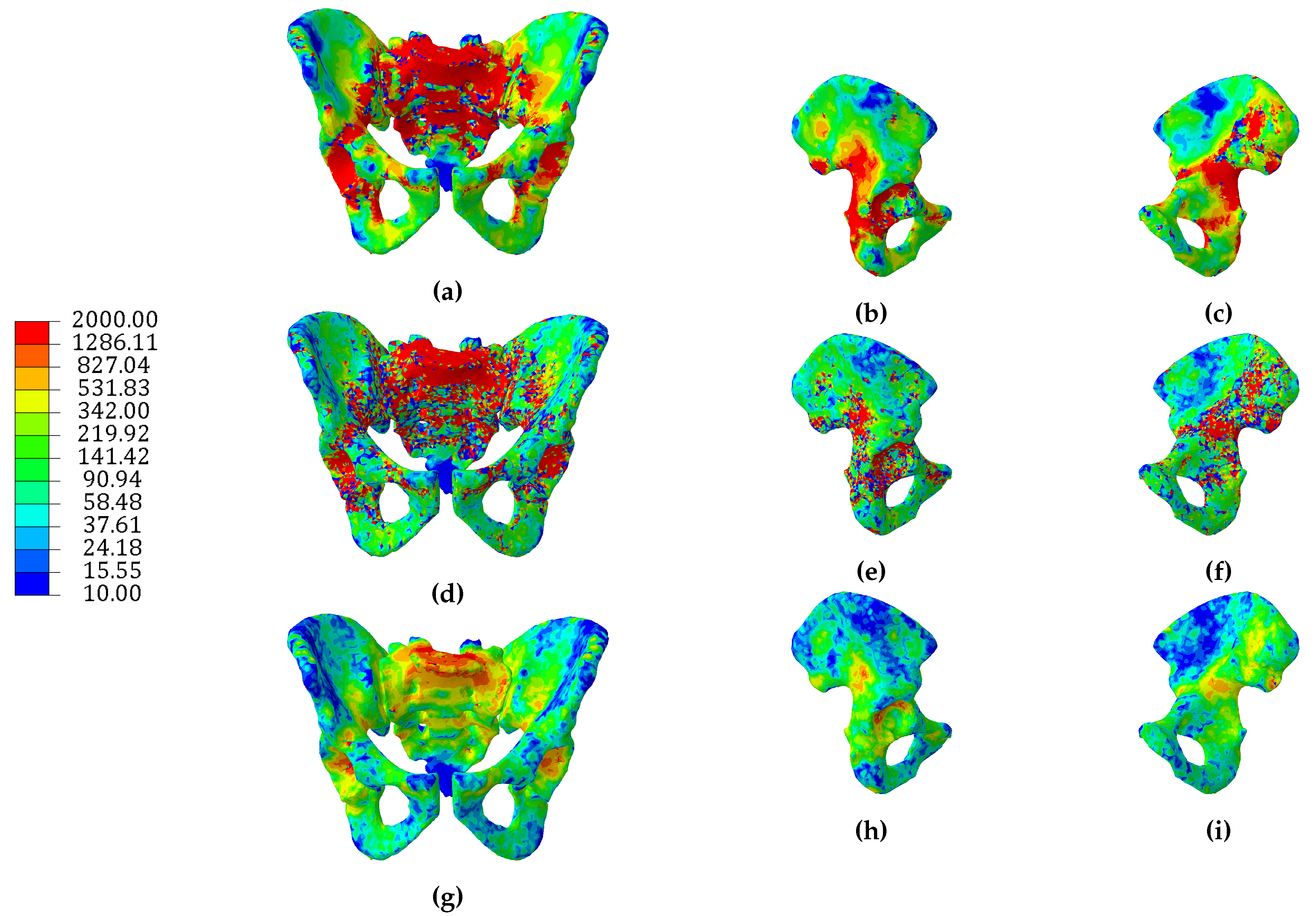
The continuum isotropic model converged to an adapted solution after 25 iterations. The Young’s modulus distribution of the converged isotropic model is shown in Figure 3a–c. Regions with high stiffness were found along the arcuate line, anterior superior sacrum, superior pubis ramus, acetabulum and near the greater sciatic notch. Conversely, large parts of the ilium, inferior pubis ramus and inferior sacrum were found to have a low stiffness.
The continuum orthotropic model of the pelvis was found to converge after 60 iterations. The distributions of the mean and dominant Young’s moduli across the model are shown in Figure 3d–i. The mean Young’s modulus for each element was calculated as the average of the three directional Young’s moduli, whereas the dominant Young’s modulus was selected as the maximum value of the three directional moduli. Regions with high mean stiffness were found around the sacroiliac joint, along the arcuate line, around the top of the sacrum, along the superior pubis ramus, in the acetabulum and between the posterior inferior iliac spine and greater sciatic notch. Low mean stiffnesses were found at the iliac fossa, ischial tuberosity and inferior sacrum. Both models produced trabecular distributions which were broadly consistent with previous findings [9].
Visually, the distributions of isotropic Young’s modulus and orthotropic dominant Young’s modulus share more similarities than with the distribution of mean orthotropic Young’s modulus. Although the CT scan derived model has generally a higher stiffness across the whole surface compared to the adaptive continuum models, an interesting aspect to note is a region at the top of the ilium medially where the dominant Young’s modulus values of the orthotropic model were similar to the same region in the CT scan derived model. In addition, the same region appeared to have a lower stiffness in the case of the isotropic model.
A frequency distribution of Young’s modulus values for the orthotropic model, isotropic model and CT scan derived model suggests that both predictive models have similar distributions of elastic moduli, with over 75% of elements having a stiffness lower than 2 GPa. On the other hand, the CT derived model had less than 50% of elements with a stiffness lower than 2 GPa (Table 2).
3.2. Hybrid Continuum Models
The hybrid isotropic model reached a state of convergence after 24 iterations. The cortical thickness distribution is shown in Figure 4a–c . Shell elements were the thickest at the superior sacrum, along the arcuate line, around the sacroiliac joint, along the superior pubic ramus and in the region of the greater sciatic notch. Areas with thin shell elements were found on the superior ilium, inferior pubic ramus, ischial tuberosity, pubic tubercle and supraacetabular region.
The Young’s modulus distribution of the continuum elements in the hybrid isotropic model are shown in Figure 5a–c. Regions with high stiffness were found along the arcuate line, anterior superior sacrum, superior pubis ramus, acetabulum and near the greater sciatic notch. Conversely, large parts of the ilium, inferior pubis ramus and inferior sacrum were found to have a low stiffness.
The hybrid orthotropic model of the pelvis was found to converge after 44 iterations. The cortical thickness distribution is illustrated in Figure 4d–f. Thick shell elements appeared at the superior sacrum, around the sacroiliac joint, along the superior pubic ramus and in the region of the greater sciatic notch. Areas with thin shell elements were found on the superior ilium, inferior pubic ramus, ischial tuberosity and supraacetabular region.
The distribution of mean and dominant Young’s moduli of the continuum elements of the hybrid orthotropic model is shown in Figure 5d–i. Regions with high Young’s moduli were found around the sacroiliac joint, on the arcuate line close to the sacrum, around the top of the sacrum, along the superior pubis ramus, around the superior acetabulum and between the posterior inferior iliac spine and greater sciatic notch. Low Young’s moduli were found at the iliac fossa, ischial tuberosity, inferior sacrum and superior ilium, similar to the hybrid isotropic model. Similar to the distributions of the continuum models, distributions of dominant Young’s moduli of the hybrid orthotropic model were visually more similar to the distributions of isotropic Young’s moduli than the distributions of orthotropic mean Young’s moduli.
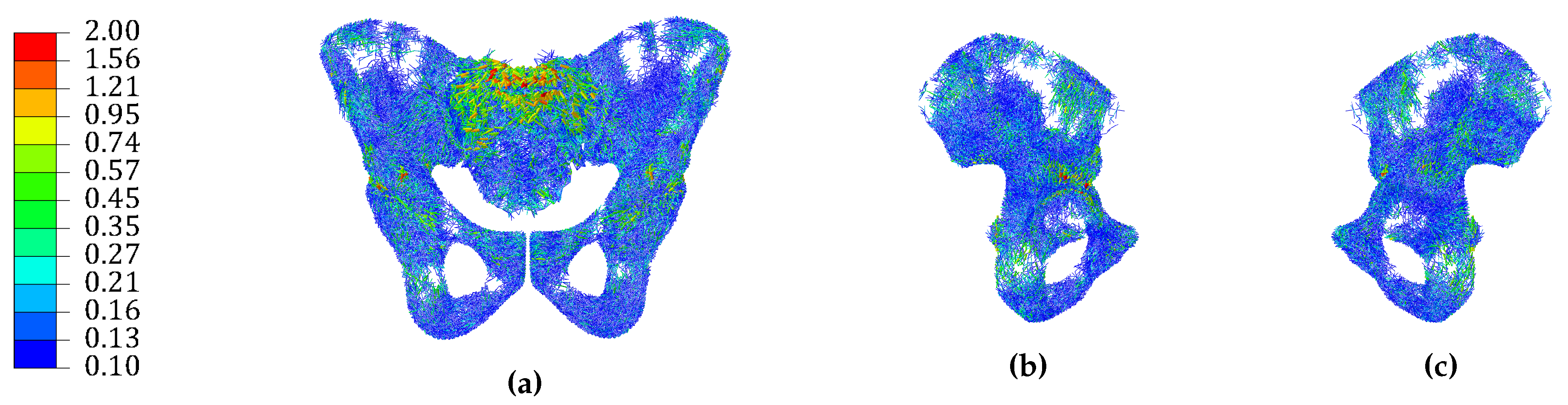
A structural model previously developed by the authors [39] was included in this comparison. Cortical thickness was highest at the superior sacrum, along the gluteal surface, around the sacroiliac joint, superior pubic ramus, posterior iliac crest and greater sciatic notch. Cortical bone had a thickness between 0.1 mm and 0.5 mm at the ischium, acetabulum, pubic tubercle, iliac fossa and posterior superior iliac spine (Figure 4g–i). The main differences between the structural model and the hybrid continuum models in terms of cortical thickness distribution were found on the ilium superior to the acetabular region, where the structural model predicted an increase in cortical thickness with respect to the hybrid continuum models, and in the area of the sacroiliac joint, where both hybrid continuum models predicted cortical thickness close to the upper limit, whereas the structural model predicted lower thicknesses, with a few elements 5 mm thick.
Clusters of elements with large radii were found at the superior sacrum, supra acetabular region, pubic tubercle and greater sciatic notch. Regions with a small number of active elements were found at the iliac fossa, ischial tuberosity and inferior sacrum (Figure 6). The trabecular architecture predicted by the structural model was visually similar to the trabecular stiffness distributions predicted by the hybrid continuum models, particularly at the top of the sacrum, iliac crest, above the sciatic notch and in the acetabular region.
Frequency distributions of the trabecular Young’s moduli for the hybrid orthotropic and hybrid isotropic models are shown in Table 3. Over 80% of elements in the hybrid orthotropic model had at least one directional elastic modulus lower than 200 MPa, whereas the Young’s modulus values of the hybrid isotropic model were more distributed, with consistently more elements than the hybrid orthotropic model for values ranging from 200 MPa to 2000 MPa.
The frequency distribution of the cortical shell thickness across the hybrid models is shown in Table 4, along with the cortical thickness distribution of the structural model. The thickness distributions of the hybrid models were largely similar, whereas the structural model had a greater number of thicker shell elements. This difference can be attributed to the hybrid models having continuum elements in contact with the shell, taking a larger proportion of the surface loading as opposed to the truss elements of the structural model.
3.3. Comparison to CT Scan Derived Model
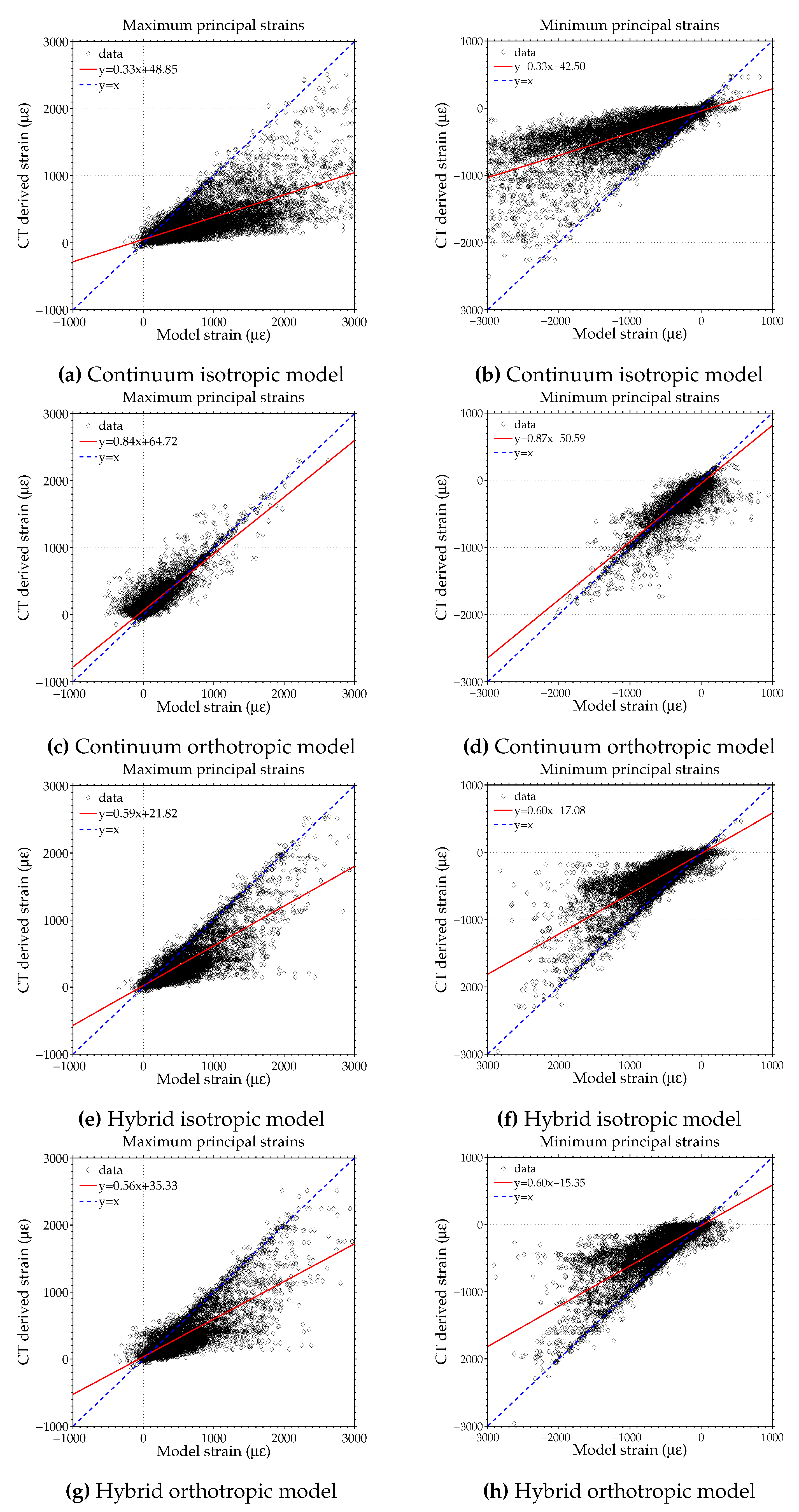
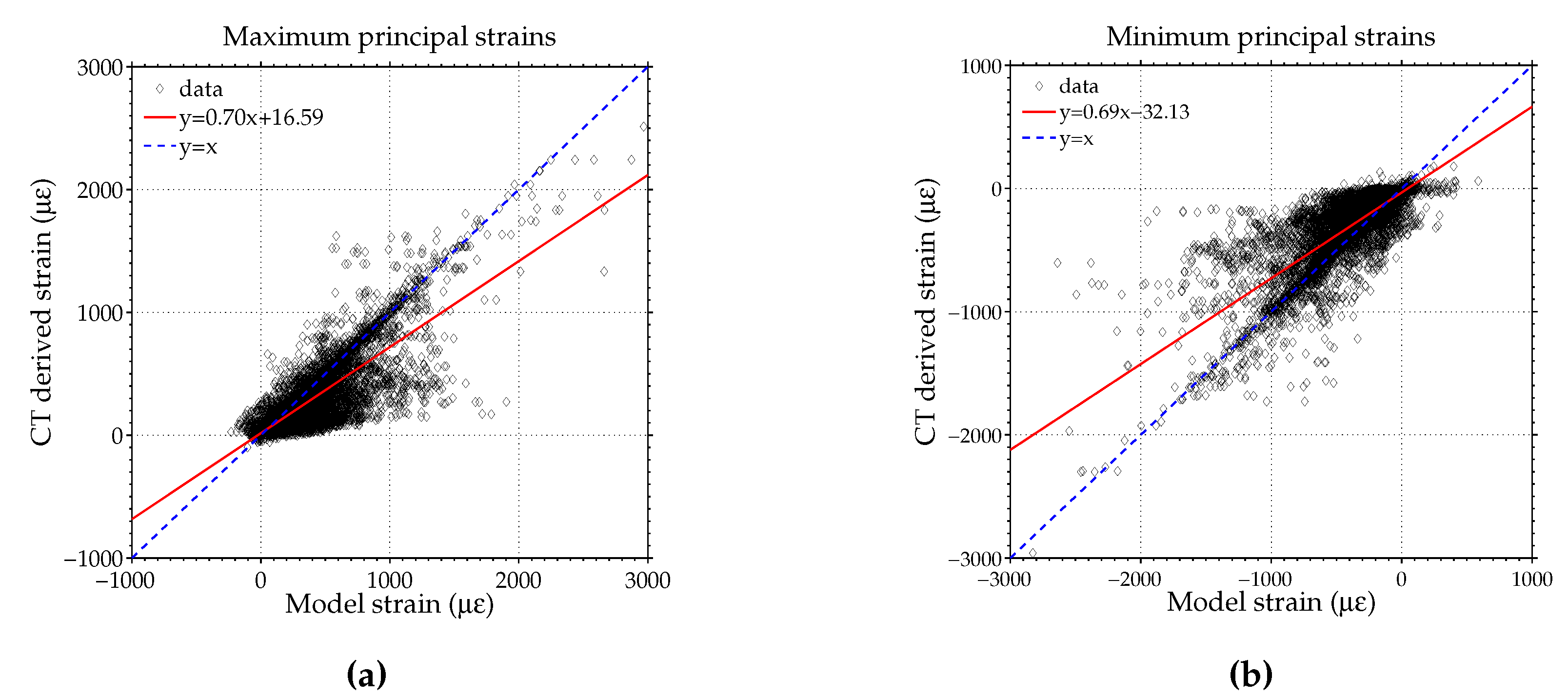
The minimum and maximum principal strains on the surface of each model as a result of a loading scenario associated with upright standing (described in Zaharie and Phillips [39]) were compared to the homologous strains for the CT scan derived model subjected to the same loading scenario (Figure 7 and Figure 8). The plots indicate that the continuum isotropic model had the worst match with the CT scan derived model, whereas the continuum orthotropic model had the best match. Both hybrid continuum models compared similarly to the CT scan derived model. Finally, the structural model was found to have the second best match in terms of fit, with a clustering of elements more similar to the hybrid models than the continuum models, indicating that the inclusion of a shell has a considerable effect on the overall stiffness of the models.
The determination coefficients and gradients of lines of best fit between each adaptive model and the CT scan derived model are shown in Table 5. Values of gradient below 1 indicate that the adapted model is less stiff than the CT scan derived model. In addition, determination coefficients and gradients of lines of best fit between each pair of adaptive models are shown in Table 6 and Table 7.
Bone volumes of each model were calculated and, where applicable, were divided into cortical and trabecular volumes (Table 8). For the continuum models, relative density and volume were calculated for each element, with their product giving a bone volume value. The relative density of each element was derived from the Young’s modulus using an approach developed by Geraldes et al. [15], described in the electronic supplementary material of that study. Total bone volume was obtained by summing bone volumes of all elements. The volumes of structural elements were calculated without having to take into account relative density. The CT scan derived model had a much higher volume of bone compared to any of the adapted models.
4. Discussion
The current study sought to compare different FE modelling approaches to simulate bone adaptation in the pelvic construct. A number of computational models were developed and subjected to an iterative adaptation in response to a loading environment associated with physical activities of daily life. The converged models were compared in terms of the predicted bone architecture and response to an upright standing load case along with a CT scan derived continuum model and a previously developed structural model [39]. The converged models and the CT scan derived model are freely available in the Supplementary Materials.
Both continuum models had a much greater number of low stiffness elements present compared to CT data (Table 2). Although the average stiffness of the orthotropic model (819.2 MPa) was lower than both the isotropic and CT derived models’ average stiffnesses (1689 MPa and 3728 MPa, respectively), its behaviour under loading was more similar to the CT derived model than the isotropic model (Table 5). This can be attributed to the directional material properties of the orthotropic model, which allows regions of bone to have different stiffnesses in different directions. This approach enables the use of less bone material while maintaining a higher overall directional stiffness, compared to an isotropic approach, similar to the findings of Geraldes and Phillips [14]. In addition, dominant Young’s modulus values in the elements of the orthotropic model increase their stiffness (average 2161 MPa) compared to the isotropic model, whereas the mean Young’s modulus values of the orthotropic model are lower than the corresponding values in the isotropic model. An important aspect to consider regarding the stiffness of the adaptive models is the target strain used to drive bone adaptation, as a lower target strain value would result in stiffer models.
The two hybrid models presented in this study were developed with the objective of differentiating between cortical and trabecular bone by using different element types. Interestingly, both hybrid models fared similarly when compared to the CT derived model (Table 5), meaning that the addition of a layer of shell elements to represent the cortex reduced the effect of considering the orthotropy of cancellous bone. An explanation can be provided by the change in the elastic modulus distributions for the continuum isotropic models, where more elements had a Young’s modulus closer to the upper limit for the hybrid isotropic model than the continuum isotropic model. Conversely, the distribution of Young’s moduli for the continuum and hybrid orthotropic models were largely similar. In addition, there were few discrepancies in the cortical thickness distributions of the two hybrid models (Table 4). The inclusion of shell elements to represent cortical bone seemed to reduce the importance of deciding between isotropic and orthotropic properties assigned to trabecular bone when comparing resulting bone architectures and overall stiffness of models.
A structural model previously developed by the authors [39] was included in this study to assess how a structural approach compared against continuum and hybrid approaches. The structural model compared well to the CT scan derived model, with only the continuum orthotropic model predicting a closer response (Table 5). Although the coefficients of determination for the structural model were lower than for both hybrid models, the gradient of the line of best fit was higher, indicating a better stiffness match with the CT scan derived model. Interestingly, the hybrid orthotropic model and structural model were found to be very similar (Table 6 and Table 7), suggesting that both approaches result in similar directionality dependent behaviour and both can be used in the design of bone scaffold structures. In addition, a structural representation of the trabecular bone provides a clear image of bone architecture, suggesting that this approach is capable of picking up trabecular motifs present in bone.
The total bone volume of the CT scan derived model was much greater than any of the adapted models (Table 8). A reason for this discrepancy could be attributed to the adaptation algorithm being set up to generate the minimum amount of bone required to sustain the load cases tested. In addition, the selected load cases do not capture the full loading environment that a pelvis is subjected to and develops in throughout its lifetime, including strenuous activities such as running, which would result in higher muscle and joint contact forces. The disappearance of bone in the dead zone was modelled as instantaneous in the algorithm, whereas, in reality, this process is time dependent.
In addition, the grayscale values defining the material distribution of the CT scan model might overestimate the true stiffness of local regions. At the scale of clinical CT imaging, directional stiffnesses are not clearly defined which can lead to inaccuracies when quantifying the stiffness using a single isotropic value.
The modelling framework presented in this study has a number of limitations that must be acknowledged. In the musculoskeletal model used to derive the loading environment applied on the pelvis, muscle actuators did not take into account contraction dynamics and force-length-velocity relationships [49]. Furthermore, the muscle actuators were not spread over bone attachment areas and compressive forces of muscles applied on bone were not taken into account. This limitation was partially overcome by having a large number of muscle actuators in the musculoskeletal model. The FE model was developed to contain only bone, ligaments and cartilage. The lack of internal organs and soft tissue associated with the pelvic region could have an impact on the resulting bone architecture in some regions. A potential limitation of the FE models is the scale at which they were developed. The average edge length of the continuum elements was 3.76 mm, closer to the macroscale rather than the microscale, as discussed in the supplementary material in Zaharie and Phillips [39]. In addition, this scale would not allow for bone voids to be modelled. However, the adapted models could potentially allow for assessment of bone voids and bone microarchitecture using macro-to-micro conversion relationships [54].
The lack of separate cortical and trabecular bone representations in the continuum models can be a hindrance in the cases when bone architecture needs to be assessed locally. Similarly, the resolution of the clinical CT scan was not suitable to allow cortical bone to be distinguished from trabecular bone throughout the pelvis. Although the hybrid continuum models overcome this limitation, they do not provide sufficient information on bone architecture. The hybrid orthotropic model provides trabecular bone directionality in addition to the hybrid isotropic model, but it does not allow for an assessment of trabecular bone architecture locally. This capability is provided by the structural model. On the other hand, the high stiffness of the shell elements in the hybrid and structural models followed immediately by elements with lower stiffness can pose a limitation as moments that may be present in the cortex might not be transferred to the trabecular bone in its vicinity.
All models were found to have run times of approximately three minutes for a single loadcase on a workstation PC with one Intel Xeon E5-2630 v2 2.60 GHz (Dell Computer Corporation, Round Rock, TX, USA) and 64 GB of RAM. The overall run times for adapting the models to the full loading regime were approximately 24 h for the isotropic model, 40 h for the orthotropic model, 25 h for the hybrid isotropic model and 38 h for the hybrid orthotropic model. The continuum and hybrid isotropic models reported similar runtimes to the structural model. The main factor in slowing down the adaptation of the orthotropic and hybrid orthotropic models was post-processing. Adapting a model with a much finer mesh to the same loading regime would result in a longer runtime. Thus, although the scale poses a limitation, the models are considered to present a reasonable balance between accuracy and computational efficiency.
The computational models presented in this study were developed with the purpose of simulating bone adaptation in the pelvic construct using different modelling approaches and material models and comparing the effect that different modelling approaches have on bone adaptation. A distinct advantage of using predictive modelling is the potential of gaining insight into the role of different activities and corresponding muscle loading patterns on driving bone adaptation without requiring information from CT data.
Considering that the CT derived model is isotropic, it is unexpected that those models which include directionality either through the use of structural elements or material directionality all compare more favourably with the CT derived model than the predicted isotropic continuum model. A potential explanation for this is that the conversion going from HU values in the CT images to the Young’s modulus values in the FE model picks up the dominant rather than the mean Young’s modulus. To assess this, a combined model was generated in which the material directionalities and ratios between the Young’s moduli found for the converged adapted orthotropic continuum model were imposed on the CT derived model, while setting the dominant Young’s modulus value to that given by the CT scan, resulting in an overall average stiffness of 2403 MPa. If the conversion process finds the dominant Young’s modulus value, then this combination of the predicted continuum orthotropic and CT derived model would be expected to have a similar response to the unaltered CT derived model for the single leg stance load case. The slopes of the lines of best fit for the hybrid model compared to the CT derived model are 0.96 and 0.99 for the maximum and minimum principal strains, respectively, indicating that the conversion from HU to Young’s modulus does find the dominant rather than the mean Young’s modulus.
5. Conclusions
The findings of this study suggest that material directionality plays an important factor in the balance between overall stiffness and total volume of material used in the case of the continuum and structural models. On the other hand, distinguishing between cortical and trabecular bone leads to a reduction in the effect of material directionality on overall stiffness, potentially due to the directionality imposed through the use of shell elements to represent cortical bone. In cases where distinguishing between trabecular and cortical bone is important, both hybrid approaches and the structural approach seem appropriate with the caveat that a structural approach could potentially have a further advantage of directly providing architecture that can be additively manufactured. In addition, despite using two different approaches, the orthotropic, hybrid and structural models predicted similar outcomes while the isotropic predictive model compared least favourably with the CT derived model, indicating that using an isotropic approach to model bone adaptation might not be a suitable solution.
In addition to providing information on the particularities of orthotropic and isotropic material modelling or the use of structural shell elements to model cortical bone, the adaptive models can be used to simulate the mechanical behaviour of bone seeded scaffolds designed to fill bone defects or to aid tissue regeneration. Furthermore, as the models are strain driven, they can be used with different materials to design scaffolds or implants that will be supporting the bone architecture surrounding them, as well as stimulating bone growth. The models can also be used in applications such as rehabilitation programs, informing the user on what type of physical activity is required to stimulate a specific region, or to predict the evolution of skeletal diseases, such as osteoporosis, by modifying the target strain, remodelling rate or set of activities within the adaptation process.
Supplementary Materials
The following are available at https://www.mdpi.com/2076-3417/9/16/3320/s1.
Author Contributions
Conceptualization, D.Z. and A.P.; methodology, D.Z. and A.P.; formal analysis, D.Z.; investigation, D.Z.; writing—original draft preparation, D.Z.; writing—review and editing, A.P.; supervision, D.Z.; project administration, A.P.; funding acquisition, A.P.
Funding
This work was conducted under the auspices of the Royal British Legion Centre for Blast Injury Studies at Imperial College London. The authors would like to acknowledge the financial support of the Royal British Legion.
Conflicts of Interest
The authors declare no conflict of interest. The funders had no role in the design of the study; in the collection, analyses, or interpretation of data; in the writing of the manuscript, or in the decision to publish the results.
References
- Michaeli, D.A.; Murphy, S.B.; Hipp, J.A. Comparison of predicted and measured contact pressures in normal and dysplastic hips. Med. Eng. Phys. 1997, 19, 180–186. [Google Scholar] [CrossRef]
- van den Bogert, A.J.; Read, L.; Nigg, B.M. An analysis of hip joint loading during walking, running, and skiing. Med. Sci. Sports Exerc. 1999, 31, 131–142. [Google Scholar] [CrossRef] [PubMed]
- Bergmann, G.; Deuretzabacher, G.; Heller, M.; Graichen, F.; Rohlmann, A.; Strauss, J.; Duda, G.N. Hip forces and gait patterns from rountine activities. J. Biomech. 2001, 34, 859–871. [Google Scholar] [CrossRef]
- Frost, H.M. Bone’s mechanostat: A 2003 update. Anat. Rec. Part A Discov. Mol. Cell. Evolut. Biol. 2003, 275, 1081–1101. [Google Scholar] [CrossRef] [PubMed]
- Treece, G.M.; Gee, A.H.; Mayhew, P.M.; Poole, K.E.S. High resolution cortical bone thickness measurement from clinical CT data. Med. Image Anal. 2010, 14, 276–290. [Google Scholar] [CrossRef]
- Phillips, A.T.M.; Villette, C.C.; Modenese, L. Femoral bone mesoscale structural architecture prediction using musculoskeletal and finite element modelling. Int. Biomech. 2015, 2, 43–61. [Google Scholar] [CrossRef] [Green Version]
- Jacob, H.A.C.; Huggler, A.H.; Dietschi, C.; Schreiber, A. Mechanical function of subchondral bone as experimentally determined on the acetabulum of the human pelvis. J. Biomech. 1976, 9, 625–627. [Google Scholar] [CrossRef]
- Dalstra, M.; Huiskes, R.; Odgaard, A.; van Erning, L. Mechanical and textural properties of pelvic trabecular bone. J. Biomech. 1993, 26, 523–535. [Google Scholar] [CrossRef] [Green Version]
- Anderson, A.E.; Peters, C.L.; Tuttle, B.D.; Weiss, J.A. Subject-Specific Finite Element Model of the Pelvis: Development, Validation and Sensitivity Studies. J. Biomech. Eng. 2005, 127, 364. [Google Scholar] [CrossRef]
- Giorgi, M.; Verbruggen, S.W.; Lacroix, D. In silico bone mechanobiology: Modeling a multifaceted biological system. Wiley Interdiscip. Rev. Syst. Biol. Med. 2016, 8, 485–505. [Google Scholar] [CrossRef]
- Wang, L.; Dong, J.; Xian, C.J. Computational modeling of bone cells and their biomechanical behaviors in responses to mechanical stimuli. Crit. Rev. Eukaryot. Gene Expr. 2019, 29, 51–67. [Google Scholar] [CrossRef] [PubMed]
- Tsubota, K.I.; Suzuki, Y.; Yamada, T.; Hojo, M.; Makinouchi, A.; Adachi, T. Computer simulation of trabecular remodeling in human proximal femur using large-scale voxel FE models: Approach to understanding Wolff’s law. J. Biomech. 2009, 42, 1088–1094. [Google Scholar] [CrossRef] [PubMed]
- Geraldes, D.; Phillips, A. A novel 3d strain-adaptive continuum orthotropic bone remodelling algorithm: prediction of bone architecture in the femur. In Proceedings of the 6th World Congress of Biomechanics (WCB 2010), Singapore, 1–6 August 2010; Springer: Berlin, Germany, 2010; pp. 772–775. [Google Scholar]
- Geraldes, D.M.; Phillips, A. A comparative study of orthotropic and isotropic bone adaptation in the femur. Int. J. Numer. Methods Biomed. Eng. 2014, 30, 873–889. [Google Scholar] [CrossRef] [PubMed] [Green Version]
- Geraldes, D.M.; Modenese, L.; Phillips, A.T. Consideration of multiple load cases is critical in modelling orthotropic bone adaptation in the femur. Biomech. Model. Mechanobiol. 2016, 15, 1029–1042. [Google Scholar] [CrossRef] [PubMed]
- Marzban, A.; Nayeb-Hashemi, H.; Vaziri, A. Numerical simulation of load-induced bone structural remodelling using stress-limit criterion. Comput. Methods Biomech. Biomed. Eng. 2015, 18, 259–268. [Google Scholar] [CrossRef] [PubMed]
- Villette, C.C.; Phillips, A.T. Informing phenomenological structural bone remodelling with a mechanistic poroelastic model. Biomech. Model. Mechanobiol. 2016, 15, 69–82. [Google Scholar] [CrossRef] [PubMed]
- Villette, C.; Phillips, A. Microscale poroelastic metamodel for efficient mesoscale bone remodelling simulations. Biomech. Model. Mechanobiol. 2017, 16, 2077–2091. [Google Scholar] [CrossRef] [Green Version]
- Goel, V.K.; Valliappan, S.; Svensson, N.L. Stresses in the normal pelvis. Comput. Biol. Med. 1978, 8, 91–104. [Google Scholar] [CrossRef]
- Oonishi, H.; Isha, H.; Hasegawa, T. Mechanical analysis of the human pelvis and its application to the artificial hip joint–by means of the three-dimensional, finite element method. J. Biomech. 1983, 16, 427–444. [Google Scholar] [CrossRef]
- Landjerit, B.; Jacquard-Simon, N.; Thourot, M.; Massin, P. Physiological loadings on human pelvis: A comparison between numerical and experimental simulations. Proc. ESB 1992, 8, 195. [Google Scholar]
- Schuller, H.; Dalstra, M.; Huiskes, R.; Marti, R. Total hip reconstruction in acetabular dysplasia. A finite element study. J. Bone Joint Surg. Br. 1993, 75B, 468–474. [Google Scholar] [CrossRef]
- Pedersen, D.R.; Crowninshield, R.D.; Brand, R.A.; Johnston, R.C. An axisymmetric model of acetabular components in total hip arthroplasty. J. Biomech. 1982, 15, 305–315. [Google Scholar] [CrossRef]
- Huiskes, R. Finite element analysis of acetabular reconstruction. Noncemented threaded cups. Acta Orthop. Scand. 1987, 58, 620–625. [Google Scholar] [CrossRef] [PubMed]
- Vasu, R.; Carter, D.R.; Harris, W.H. Stress distributions in the acetabular region-I. Before and after total joint replacement. J. Biomech. 1982, 15, 155–157. [Google Scholar] [CrossRef]
- Carter, D.R.; Vasu, R.; Harris, W.H. Stress distributions in the acetabular region-II. Effects of cement thickness and metal backing of the total hip acetabular component. J. Biomech. 1982, 15, 165–170. [Google Scholar] [CrossRef]
- Rapperport, D.; Carter, D.; Schurman, D. Contact finite element stress analysis of the hip joint. J. Orthop. Res. 1985, 3, 435–446. [Google Scholar] [CrossRef] [PubMed]
- Oonishi, H.; Tatsumi, M.; Kawaguchi, A. Biomechanical studies on fixations of an artificial hip joint acetabular socket by means of 2D-FEM. In Biological and Biomechanical Performance of Biomaterials; Christel, P., Meunier, A., Lee, A.J.C., Eds.; Elsevier: Amsterdam, The Netherlands, 1986; pp. 513–518. [Google Scholar]
- Phillips, A.T.M.; Pankaj, P.; Usmani, A.S.; Howie, C.R. Numerical modelling of the acetabular construct following impaction grafting. In Proceedings of the International Symposium on Computer Methods in Biomechanics and Biomedical Engineering, Madrid, Spain, 25–28 February 2004. [Google Scholar]
- Dalstra, M.; Huiskes, R.; van Erning, L. Development and validation of a three-dimensional finite element model of the pelvic bone. J. Biomech. Eng. 1995, 117, 272–278. [Google Scholar] [CrossRef]
- Li, Z.; Kim, J.E.; Davidson, J.S.; Etheridge, B.S.; Alonso, J.E.; Eberhardt, A.W. Biomechanical response of the pubic symphysis in lateral pelvic impacts: a finite element study. J. Biomech. 2007, 40, 2758–2766. [Google Scholar] [CrossRef] [PubMed]
- Zhang, Q.H.; Wang, J.Y.; Lupton, C.; Heaton-Adegbile, P.; Guo, Z.X.; Liu, Q.; Tong, J. A subject-specific pelvic bone model and its application to cemented acetabular replacements. J. Biomech. 2010, 43, 2722–2727. [Google Scholar] [CrossRef]
- Pankaj, P. Patient-specific modelling of bone and bone-implant systems: the challenges. Int. J. Numer. Methods Biomed. Eng. 2013, 29, 233–249. [Google Scholar] [CrossRef]
- Ashman, R.; Cowin, S.; Van Buskirk, W.; Rice, J. A continuous wave technique for the measurement of the elastic properties of cortical bone. J. Biomech. 1984, 17, 349–361. [Google Scholar] [CrossRef]
- Morlock, M.; Schneider, E.; Bluhm, A.; Vollmer, M.; Bergmann, G.; Müller, V.; Honl, M. Duration and frequency of every day activities in total hip patients. J. Biomech. 2001, 34, 873–881. [Google Scholar] [CrossRef]
- Modenese, L.; Gopalakrishnan, A.; Phillips, A. Application of a falsification strategy to a musculoskeletal model of the lower limb and accuracy of the predicted hip contact force vector. J. Biomech. 2013, 46, 1193–1200. [Google Scholar] [CrossRef] [PubMed]
- Horsman, M.D.K.; Koopman, H.; der Helm, F.C.T.; Prosé, L.P.; Veeger, H.E.J. Morphological muscle and joint parameters for musculoskeletal modelling of the lower extremity. Clin. Biomech. 2007, 22, 239–247. [Google Scholar] [CrossRef] [PubMed]
- Delp, S.; Anderson, F.; Arnold, A.; Loan, P.; Habib, A.; John, C.; Guendelman, E.; Thelen, D. OpenSim: Open source to create and analyze dynamic simulations of movement. IEEE Trans. Biomed. Eng. 2007, 54, 1940–1950. [Google Scholar] [CrossRef]
- Zaharie, D.T.; Phillips, A.T. Pelvic construct prediction of trabecular and cortical bone structural architecture. J. Biomech. Eng. 2018, 140, 091001. [Google Scholar] [CrossRef] [PubMed]
- Barre, A.; Armand, S. Biomechanical ToolKit: Open-source framework to visualize and process biomechanical data. Comput. Methods Programs Biomed. 2014, 114, 80–87. [Google Scholar] [CrossRef]
- Dumas, R.; Chèze, L.; Verriest, J.P. Adjustments to McConville et al. and Young et al. body segment inertial parameters. J. Biomech. 2007, 40, 543–553. [Google Scholar] [CrossRef]
- Lu, T.W.; O’Connor, J.J. Bone position estimation from skin marker co-ordinates using global optimisation with joint constraints. J. Biomech. 1999, 32, 129–134. [Google Scholar] [CrossRef]
- van Arkel, R.J.; Modenese, L.; Phillips, A.T.; Jeffers, J.R. Hip abduction can prevent posterior edge loading of hip replacements. J. Orthop. Res. 2013, 31, 1172–1179. [Google Scholar] [CrossRef] [Green Version]
- Steele, K.M.; DeMers, M.S.; Schwartz, M.H.; Delp, S.L. Compressive tibiofemoral force during crouch gait. Gait Posture 2012, 35, 556–560. [Google Scholar] [CrossRef] [Green Version]
- Phillips, A.; Pankaj, P.; Howie, C.; Usmani, A.; Simpson, A. Finite element modelling of the pelvis: Inclusion of muscular and ligamentous boundary conditions. Med. Eng. Phys. 2007, 29, 739–748. [Google Scholar] [CrossRef]
- Hammer, N.; Steinke, H.; Slowik, V.; Josten, C.; Stadler, J.; Böhme, J.; Spanel-Borowski, K. The sacrotuberous and the sacrospinous ligament—A virtual reconstruction. Ann. Anat. Anat. Anz. 2009, 191, 417–425. [Google Scholar] [CrossRef]
- Hammer, N.; Steinke, H.; Böhme, J.; Stadler, J.; Josten, C.; Spanel-Borowski, K. Description of the iliolumbar ligament for computer-assisted reconstruction. Ann. Anat. Anat. Anz. 2010, 192, 162–167. [Google Scholar] [CrossRef]
- Moore, K.L.; Agur, A.M.R.; Dalley, A.F.; Moore, K.L. Essential Clinical Anatomy; Wolters Kluwer Health: Alphen aan den Rijn, The Netherlands, 2015. [Google Scholar]
- Modenese, L.; Phillips, A.T.M.; Bull, A.M.J. An open source lower limb model: Hip joint validation. J. Biomech. 2011, 44, 2185–2193. [Google Scholar] [CrossRef] [Green Version]
- Phillips, A.T.M. Structural optimisation: Biomechanics of the femur. Proc. ICE Eng. Comput. Mech. 2012, 165, 147–154. [Google Scholar] [CrossRef]
- Taddei, F.; Schileo, E.; Helgason, B.; Cristofolini, L.; Viceconti, M. The material mapping strategy influences the accuracy of CT-based finite element models of bones: An evaluation against experimental measurements. Med. Eng. Phys. 2007, 29, 973–979. [Google Scholar] [CrossRef]
- Les, C.; Keyak, J.; Stover, S.; Taylor, K.; Kaneps, A. Estimation of material properties in the equine metacarpus with use of quantitative computed tomography. J. Orthop. Res. 1994, 12, 822–833. [Google Scholar] [CrossRef]
- Keller, T.S. Predicting the compressive mechanical behavior of bone. J. Biomech. 1994, 27, 1159–1168. [Google Scholar] [CrossRef]
- Teo, J.C.; Si-Hoe, K.M.; Keh, J.E.; Teoh, S.H. Relationship between CT intensity, micro-architecture and mechanical properties of porcine vertebral cancellous bone. Clin. Biomech. 2006, 21, 235–244. [Google Scholar] [CrossRef]
Figure 1.
Orientation of element updated based on the principal stress directions of guiding frame.

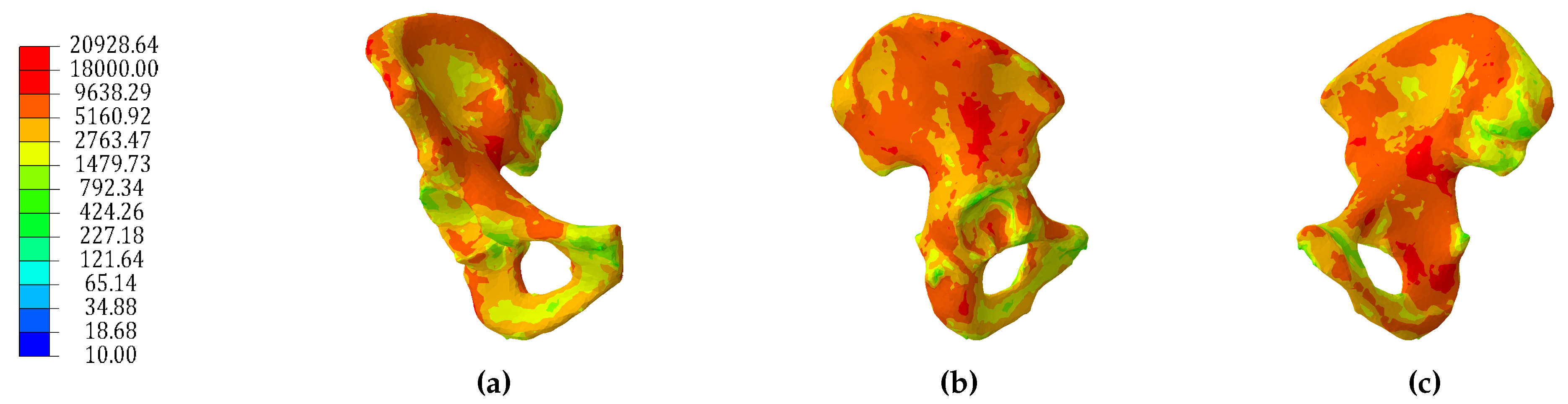
Figure 2.
Distribution of Young’s modulus (MPa) across the CT scan derived model - shown for (a) frontal, (b) lateral, and (c) medial views.
Figure 2.
Distribution of Young’s modulus (MPa) across the CT scan derived model - shown for (a) frontal, (b) lateral, and (c) medial views.

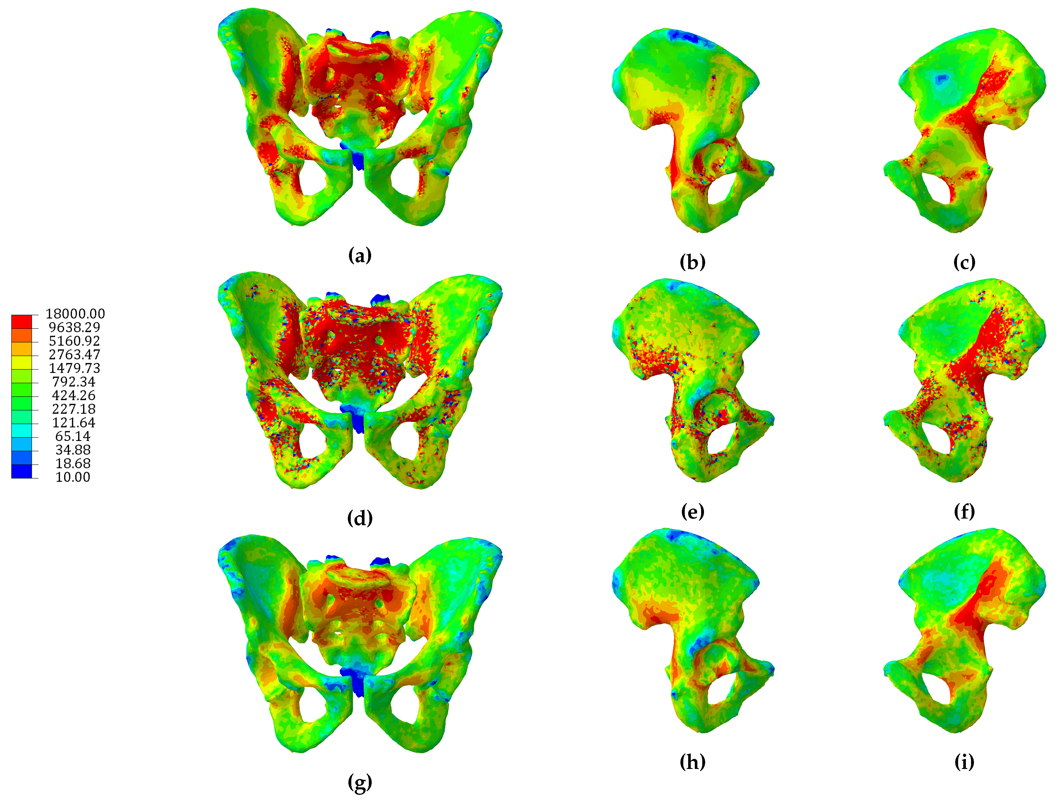
Figure 3.
Distributions of Young’s modulus (MPa) for the isotropic model (a–c), dominant Young’s modulus (d–f) and mean Young’s modulus (g–i) for the orthotropic model.
Figure 3.
Distributions of Young’s modulus (MPa) for the isotropic model (a–c), dominant Young’s modulus (d–f) and mean Young’s modulus (g–i) for the orthotropic model.

Figure 4.
Distributions of cortical thickness (mm) for the hybrid isotropic model (a–c), hybrid orthotropic model (d–f) and structural model (g–i).
Figure 4.
Distributions of cortical thickness (mm) for the hybrid isotropic model (a–c), hybrid orthotropic model (d–f) and structural model (g–i).

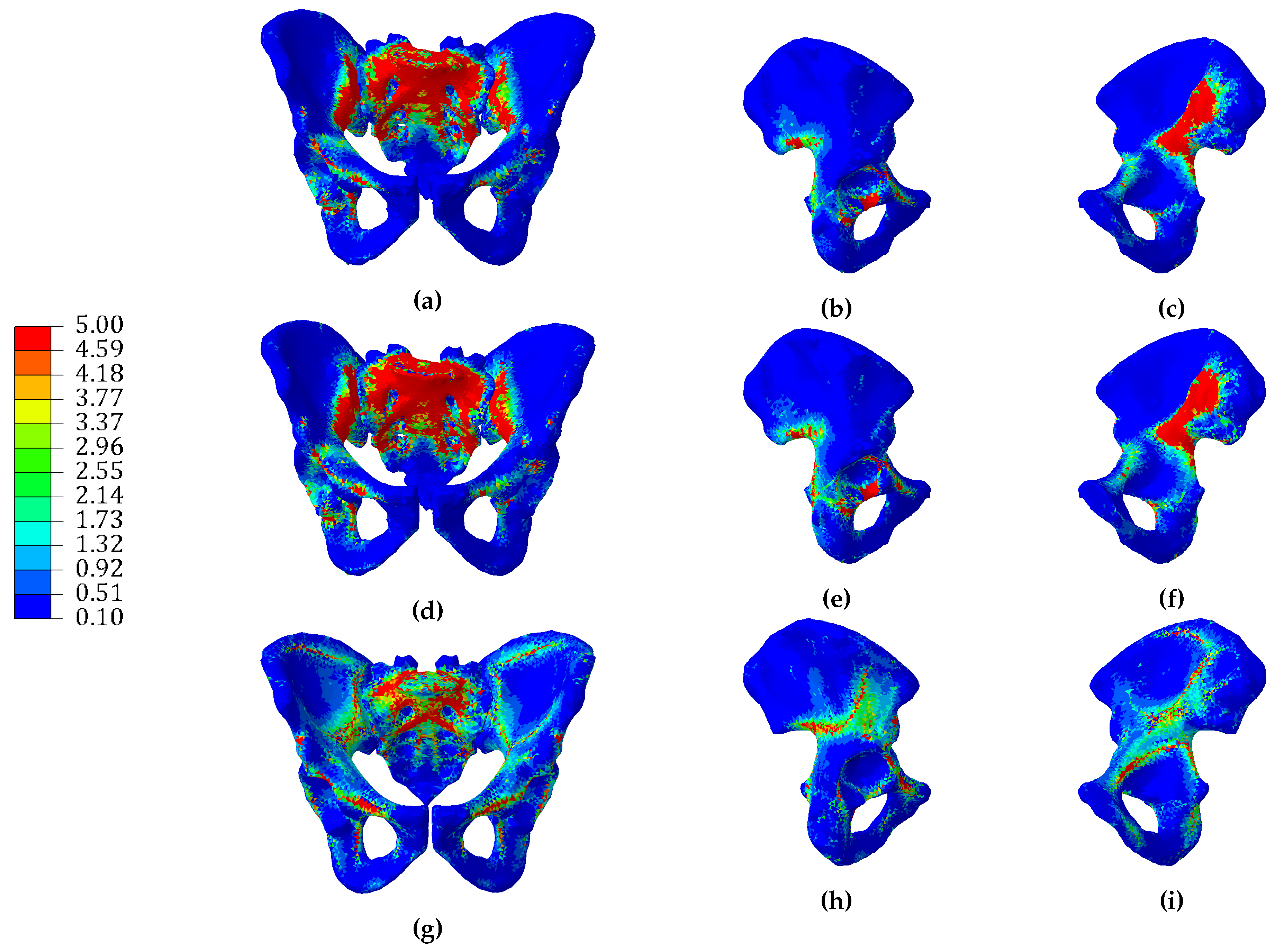
Figure 5.
Distributions of trabecular Young’s modulus (MPa) for the hybrid isotropic model (a–c), dominant Young’s modulus (d–f) and mean Young’s modulus (g–i) for the hybrid orthotropic model.
Figure 5.
Distributions of trabecular Young’s modulus (MPa) for the hybrid isotropic model (a–c), dominant Young’s modulus (d–f) and mean Young’s modulus (g–i) for the hybrid orthotropic model.

Figure 6.
Trabecular elements’ radii distribution (mm) of the structural model - shown for (a) frontal, (b) lateral, and (c) medial views. Trabecular elements with a radius <0.1 mm were excluded for clarity.
Figure 6.
Trabecular elements’ radii distribution (mm) of the structural model - shown for (a) frontal, (b) lateral, and (c) medial views. Trabecular elements with a radius <0.1 mm were excluded for clarity.

Figure 7.
Comparison between the maximum (a,c,e,g) and minimum (b,d,f,h) principal strains across the surface of the continuum and hybrid models (x-axis) and CT derived model (y-axis). Lines of best fit are shown in red for each case, with the y = x line shown in dashed blue.
Figure 7.
Comparison between the maximum (a,c,e,g) and minimum (b,d,f,h) principal strains across the surface of the continuum and hybrid models (x-axis) and CT derived model (y-axis). Lines of best fit are shown in red for each case, with the y = x line shown in dashed blue.

Figure 8.
Comparison between the maximum (a) and minimum (b) principal strains across the surface of the structural model (x-axis) and CT derived model (y-axis). Lines of best fit are shown in red for each case, with the y = x line shown in dashed blue.
Figure 8.
Comparison between the maximum (a) and minimum (b) principal strains across the surface of the structural model (x-axis) and CT derived model (y-axis). Lines of best fit are shown in red for each case, with the y = x line shown in dashed blue.


Table 1.
Element type used to model cortical and trabecular bone for each model developed.
| Model | Cortical Bone | Trabecular Bone |
|---|---|---|
| Orthotropic | Tetrahedral elements | |
| Isotropic | Tetrahedral elements | |
| Hybrid orthotropic | Shell elements | Tetrahedral elements |
| Hybrid isotropic | Shell elements | Tetrahedral elements |
| Structural | Shell elements | Truss elements |
Table 2.
Cumulative distribution (%) of elastic moduli of the three continuum models: CT scan derived, isotropic and orthotropic.
Table 2.
Cumulative distribution (%) of elastic moduli of the three continuum models: CT scan derived, isotropic and orthotropic.
| CT Scan Model | Isotropic Model | Orthotropic Model | Orthotropic Model | Orthotropic Model | Orthotropic Model | Orthotropic Model | |
|---|---|---|---|---|---|---|---|
| 10–1000 MPa | 26.32 | 63.83 | 86.33 | 91.45 | 89.37 | 71.89 | 81.79 |
| 10–2000 MPa | 47.37 | 77.88 | 89.64 | 93.89 | 92.27 | 78.85 | 87.56 |
| 10–3000 MPa | 59.48 | 84.23 | 91.44 | 95.10 | 93.74 | 82.57 | 90.43 |
| 10–5000 MPa | 73.74 | 91.01 | 93.53 | 96.39 | 95.38 | 86.82 | 93.57 |
| 10–10,000 MPa | 90.43 | 96.78 | 95.93 | 97.81 | 97.14 | 91.63 | 99.42 |
| 10–15,000 MPa | 98.51 | 98.27 | 97.14 | 98.50 | 98.01 | 94.06 | 99.97 |
| 10–18,000 MPa | 99.91 | 100.00 | 100.00 | 100.00 | 100.00 | 100.00 | 100.00 |
| Mean (MPa) | 3727.6 | 1688.7 | 1059.4 | 616.4 | 781.9 | 2161.3 | 819.2 |
| Std. dev. (MPa) | 3817.5 | 3076.9 | 3411.5 | 2559.7 | 2898.7 | 4646.9 | 1841.8 |
Table 3.
Cumulative distribution (%) of trabecular elastic moduli for the hybrid isotropic and hybrid orthotropic models.
Table 3.
Cumulative distribution (%) of trabecular elastic moduli for the hybrid isotropic and hybrid orthotropic models.
| Isotropic Model | Orthotropic Model | Orthotropic Model | Orthotropic Model | Orthotropic Model | Orthotropic Model | |
|---|---|---|---|---|---|---|
| 10–100 MPa | 33.87 | 80.06 | 87.98 | 83.05 | 59.76 | 69.44 |
| 10–200 MPa | 45.01 | 83.56 | 90.62 | 86.42 | 66.88 | 76.33 |
| 10–300 MPa | 52.78 | 85.56 | 91.99 | 88.24 | 70.84 | 80.16 |
| 10–500 MPa | 63.33 | 88.00 | 93.58 | 90.41 | 75.71 | 84.84 |
| 10–1000 MPa | 76.30 | 91.22 | 95.45 | 93.28 | 82.13 | 98.02 |
| 10–1500 MPa | 83.79 | 93.04 | 96.42 | 94.80 | 85.75 | 99.86 |
| 10–2000 MPa | 100.00 | 100.00 | 100.00 | 100.00 | 100.00 | 100.00 |
| Mean (MPa) | 585.5 | 213.3 | 121.0 | 171.0 | 422.8 | 168.5 |
| Std. dev. (MPa) | 689.1 | 522.4 | 389.1 | 461.9 | 685.9 | 281.4 |
Table 4.
Cumulative distribution of the cortical thickness for the hybrid isotropic, hybrid orthotropic and structural models.
Table 4.
Cumulative distribution of the cortical thickness for the hybrid isotropic, hybrid orthotropic and structural models.
| Isotropic Model (%) | Orthotropic Model (%) | Structural Model (%) | |
|---|---|---|---|
| 0.1–0.3 mm | 47.33 | 45.51 | 37.46 |
| 0.1–0.5 mm | 62.21 | 58.99 | 56.30 |
| 0.1–1 mm | 75.60 | 72.27 | 76.61 |
| 0.1–2 mm | 83.68 | 81.06 | 88.72 |
| 0.1–3 mm | 86.91 | 85.00 | 93.38 |
| 0.1–4 mm | 88.81 | 87.10 | 95.66 |
| 0.1–5 mm | 100.00 | 100.00 | 100.00 |
| Mean (mm) | 1.1 | 1.2 | 0.9 |
| Std. dev. (mm) | 1.5 | 1.6 | 1.1 |
Table 5.
Coefficients of determination and slopes of the line of best fit for each adaptive model compared to the CT scan derived model. A slope value of 1 means a perfect match between models.
Table 5.
Coefficients of determination and slopes of the line of best fit for each adaptive model compared to the CT scan derived model. A slope value of 1 means a perfect match between models.
| Model | εmin (R2) | εmax (R2) | εmin (Slope) | εmax (Slope) |
|---|---|---|---|---|
| Isotropic | 0.64 | 0.63 | 0.33 | 0.33 |
| Orthotropic | 0.78 | 0.79 | 0.87 | 0.84 |
| Hybrid isotropic | 0.71 | 0.72 | 0.60 | 0.59 |
| Hybrid orthotropic | 0.70 | 0.69 | 0.60 | 0.59 |
| Structural | 0.66 | 0.65 | 0.69 | 0.70 |
Table 6.
Coefficients of determination between each pair of adaptive models for maximum principal strains (above table diagonal) and minimum principal strains (below table diagonal).
Table 6.
Coefficients of determination between each pair of adaptive models for maximum principal strains (above table diagonal) and minimum principal strains (below table diagonal).
| Model | Isotropic | Orthotropic | Hybrid Isotropic | Hybrid Orthotropic | Structural |
|---|---|---|---|---|---|
| Isotropic | N/A | 0.35 | 0.81 | 0.63 | 0.62 |
| Orthotropic | 0.49 | N/A | 0.49 | 0.53 | 0.53 |
| Hybrid isotropic | 0.84 | 0.57 | N/A | 0.83 | 0.85 |
| Hybrid orthotropic | 0.63 | 0.61 | 0.81 | N/A | 0.99 |
| Structural | 0.61 | 0.61 | 0.84 | 0.99 | N/A |
Table 7.
Gradients of lines of best fit between each pair of adaptive models for maximum principal strains (above table diagonal) and minimum principal strains (below table diagonal).
Table 7.
Gradients of lines of best fit between each pair of adaptive models for maximum principal strains (above table diagonal) and minimum principal strains (below table diagonal).
| Model | Isotropic | Orthotropic | Hybrid Isotropic | Hybrid Orthotropic | Structural |
|---|---|---|---|---|---|
| Isotropic | N/A | 1.49 | 0.59 | 0.36 | 0.36 |
| Orthotropic | 1.85 | N/A | 0.97 | 0.69 | 0.7 |
| Hybrid isotropic | 0.53 | 1.07 | N/A | 1.06 | 0.71 |
| Hybrid orthotropic | 0.33 | 0.74 | 1.1 | N/A | 0.98 |
| Structural | 0.33 | 0.74 | 0.71 | 0.98 | N/A |
Table 8.
Predicted bone volumes for the adapted models and the CT scan derived model.
| Model | Cortical Bone Volume (mm3) | Trabecular Bone Volume (mm3) | E < 2 GPa (mm3) | E >2 GPa (mm3) | Total Bone Volume (mm3) |
|---|---|---|---|---|---|
| CT scan | N/A | N/A | 23269.04 | 163487.15 | 186756.20 |
| Isotropic | N/A | N/A | 25041.63 | 30499.45 | 55541.09 |
| Orthotropic | N/A | N/A | 26810.03 | 34241.34 | 61051.37 |
| Hybrid isotropic | 14941.68 | 25750.14 | N/A | N/A | 40691.82 |
| Hybrid orthotropic | 16465.59 | 17396.64 | N/A | N/A | 33862.23 |
| Structural | 17969.76 | 42321.05 | N/A | N/A | 60290.81 |
© 2019 by the authors. Licensee MDPI, Basel, Switzerland. This article is an open access article distributed under the terms and conditions of the Creative Commons Attribution (CC BY) license (http://creativecommons.org/licenses/by/4.0/).
Share and Cite
MDPI and ACS Style
Zaharie, D.T.; Phillips, A.T.M. A Comparative Study of Continuum and Structural Modelling Approaches to Simulate Bone Adaptation in the Pelvic Construct. Appl. Sci. 2019, 9, 3320. https://doi.org/10.3390/app9163320
AMA Style
Zaharie DT, Phillips ATM. A Comparative Study of Continuum and Structural Modelling Approaches to Simulate Bone Adaptation in the Pelvic Construct. Applied Sciences. 2019; 9(16):3320. https://doi.org/10.3390/app9163320
Chicago/Turabian StyleZaharie, Dan T., and Andrew T.M. Phillips. 2019. "A Comparative Study of Continuum and Structural Modelling Approaches to Simulate Bone Adaptation in the Pelvic Construct" Applied Sciences 9, no. 16: 3320. https://doi.org/10.3390/app9163320
Note that from the first issue of 2016, this journal uses article numbers instead of page numbers. See further details here.