Market Integration and Price Transmission in the Vertical Supply Chain of Rice: An Evidence from Bangladesh


1
Agricultural Economics Division, Bangladesh Rice Research Institute, Gazipur 1701, Bangladesh
2
Department of Agricultural & Resource Economics, Kangwon National University, Chuncheon 24341, Korea
*
Author to whom correspondence should be addressed.
Agriculture 2020, 10(7), 271; https://doi.org/10.3390/agriculture10070271
Submission received: 19 May 2020
/
Revised: 2 July 2020
/
Accepted: 2 July 2020
/
Published: 5 July 2020
(This article belongs to the Section Agricultural Economics, Policies and Rural Management)
Abstract
:As a staple food, rice has an enormous market in Bangladesh in terms of market participants and the volume of the product. As the price of rice is always a sensitive factor for producers, poor consumers and policy makers, this paper investigates market integration and price transmission along the vertical supply chain of rice. Johansen’s test of co-integration confirmed that farm, wholesale and retail prices are co-integrated in the long-run. A causality test revealed that prices were found to be at wholesale levels for both the upstream and downstream markets. The asymmetry error correction model (ECM) has discovered short-run and long-run asymmetry in price transmission in the vertical supply chain where both producers and consumers were being affected due to positive and negative asymmetry. Threshold autoregressive (TAR) and momentum threshold autoregressive (M-TAR) models have confirmed threshold co-integration as well as threshold effect on asymmetry in price transmission. The results highlight the inevitability of policy implementations and increased public interventions to reduce asymmetry for engendering greater pricing efficiency in Bangladesh rice markets.
1. Introduction
One key principle of several trends in economics is that markets permit price signs to be transmitted both spatially and vertically [1]. Economists have always demonstrated interest in associations between prices, even though, overall, theory claims that other variables (product features) are similarly significant in relating and explaining market equilibrium [2]. Therefore, analysis of diverse price relationships could be a decisive means for understanding market integration, or more precisely market efficiency. Studies on price transmission largely scrutinize the nature of the relationship between price series at different levels of the supply chain, or at spatially separated markets.
Rice is the staple food in Bangladesh as more than 160 million people rely on it with per capita rice consumption of 170 kg per year, while the global average is only 57 kg [3]. Rice supplies account for about 70% of caloric consumption and 58% of protein intake [3]. On the supply side, 11.7 million hectares (ha) of lands were cultivated for rice production and 35 tons (MMT) of milled rice was produced in 2018 [4]. In terms of maximum rice production, Bangladesh is ranked fourth in the world [4], which indicates the importance of rice in this country’s context. By not being a major exporter or importer, the domestic market plays a vital role in the country’s rice sector so that welfare primarily depends on the efficiency of domestic rice markets which needs to be investigated thoroughly.
A pre-requisite for producers and consumers to get advantage from this new and changing market situation is the ability of a market to function efficiently at their spatial or through the value chain dimensions which are very frequently constrained by different factors [5]. It is a common phenomenon of a developing country that its food grain marketing chains are long because of many small-scale intermediaries which make the producer prices to be lower and consumer prices to be higher, therefore resulting in the inefficient rice markets. Bangladesh is not an exception in that case while its food grain especially the rice marketing chain is dominated by several intermediaries.
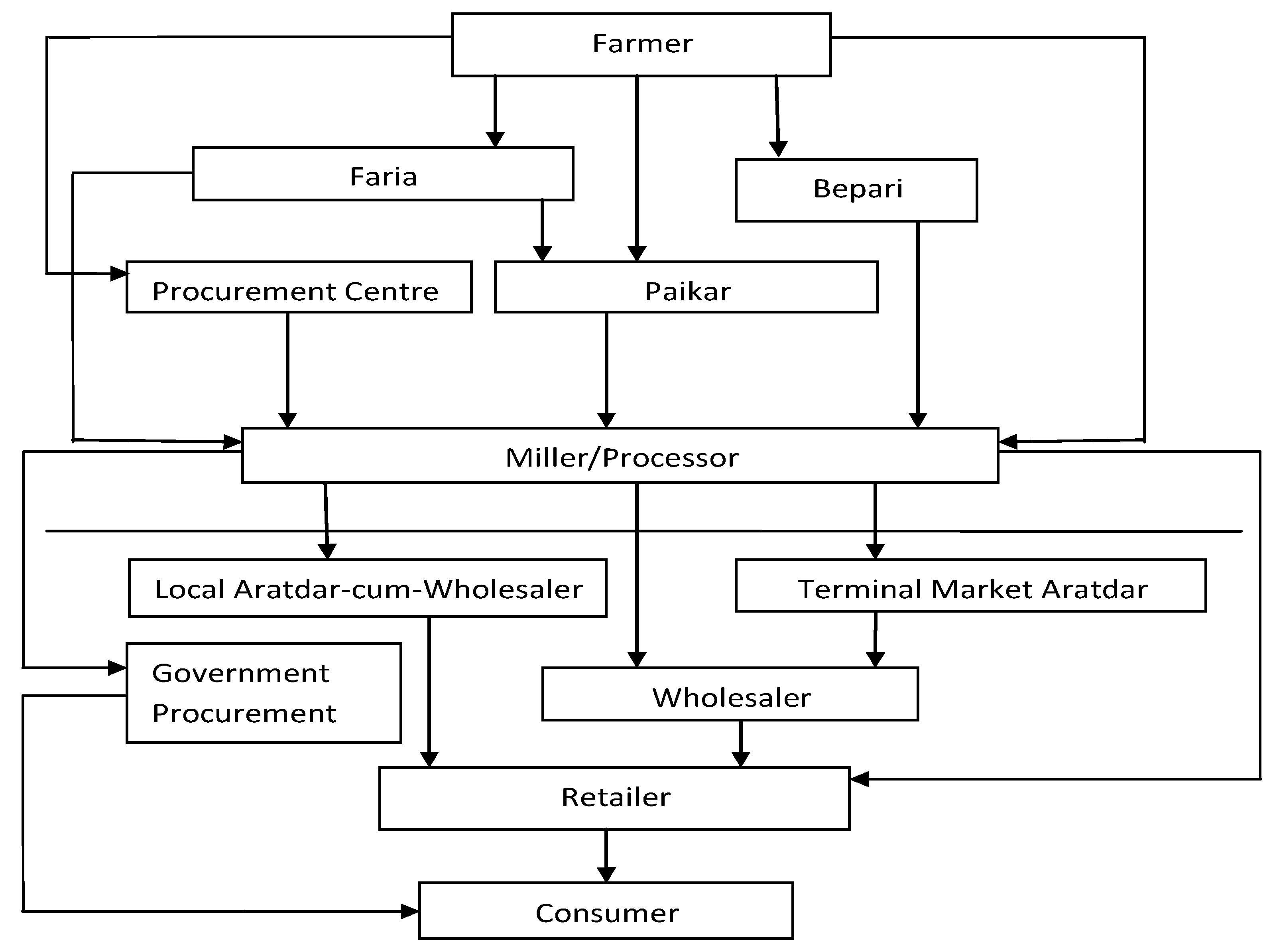
The liberalization of the rice markets in Bangladesh has significantly changed the structure of the markets [5]. Marketing channels of paddy/rice in Bangladesh are sketched in Figure 1. Faria are the primary intermediaries who work in local villages, buy paddy from farmers at farmyards and then sell it to Paikar or Millers. Bepari are primarily private traders placed in larger markets some distance away from farm areas. They are long-distance traders, who generally play some marketing roles, such as sorting, grading, packaging, etc. and supply paddy to Millers. The government also buys paddy directly from the farmers twice in a year though the amount is too little to be mentioned. Millers are the processor of paddy rice who have well-equipped processing establishments. They dry, sometimes parboil, unhusk, polish, package and even store the paddy before selling it to the Aratdar-cum-wholesaler and wholesaler at the terminal market namely Dhaka; the capital of the country and to the wholesaler as well. Sometimes they buy paddy directly from the farmers through their agents and also participate in government procurement programs. Millers especially automated rice mill owners have huge investments in the market which somehow make them influential actors in the market [6].
Aratdar-cum-wholesaler generally stay at the district or divisional level who have huge capitals or funds to run their trades; Most of them accomplish different marketing functions like buying milled rice from Millers, sorting, grading, and packing, etc. There are some terminal markets where the Aratdars perform the same activities but are located only in the capital city, Dhaka. Sometimes rice is being imported from different countries during any shortage or emergency which are bought by these Aratdars located mainly in Dhaka. The Aratdars sell milled rice to wholesalers and then wholesalers sell milled rice to retailer, who in turn sell rice to consumers. Retailers also can buy milled rice from millers and/or Aratdar-cum-wholesalers and then sell it to consumers. It is evident from the above discussion that there is no single channel moving paddy and milled rice to consumers rather than many participants that exist in the paddy/rice marketing channels along the vertical supply chain of rice in Bangladesh.
In the domestic markets, a price increase passes very quickly through the supply chain compared to a price decrease. For example, when the price of rice increases at the farm level, it is being passed immediately to the retail level and ultimately to the consumers by market intermediaries as those intermediaries show a very quick response to capture the benefit as well as avoid the risk of price rise at the producer level. But when a price decrease at the producer level, it barely affects the retail price at a quick interval of time. As a result, perception by consumers and the government exists that the market is being manipulated, raising food prices unfairly, at the expense of the poor households who are net buyers and for whom food is a major expenditure share which is about 40–50 percent [5]. Recently this issue has become more sensitive as rice farmers are not only complaining of being deprived of getting fair prices but also, they are demonstrating much disappointment which has become a very concerning issue for the Government as well. Therefore, there is a dearth of information on the nature of the price relationships in the vertical level under the existing market structure.
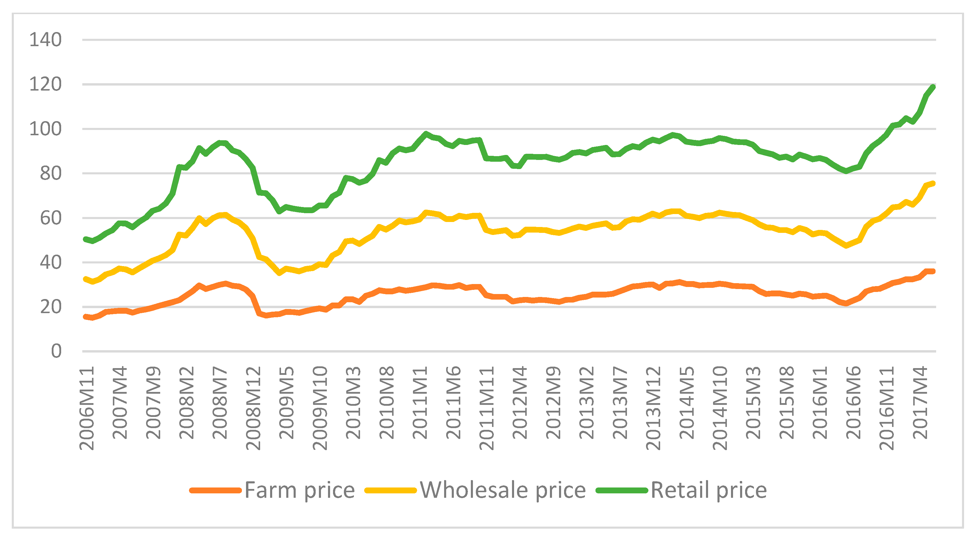
Farm, wholesale and retail prices are argued as the most distinguished level of prices along the vertical supply chain of rice in Bangladesh [5]. These three series of prices exhibit the response of producers, intermediaries and consumers who are considered as the main components in any supply chain. Figure 2 shows a plot of three distinct price series along the vertical supply chain of rice for the period November 2006 to June 2017 in Bangladesh. The graph shows some severe volatility among farm, wholesale and retail prices. These fluctuations along the years follow a similar upward trend during most of the time in the period of the analysis. There are two big changes in price from 2007 to 2008 and in 2016. From 2007 to 2008, inflation largely affected the economy in Bangladesh, especially in rice price. After the general election (29 December 2008) the prices were temporarly decreased, but chronicaaly high inflation keep influencing rice price fluctuation. Flooding reduced harvests in 2016 have increased domestic prices of rice after August 2016.
The vertical integration of grain markets plays a crucial role in improving food security and the welfare of the poor consumers. The degree and the nature of integration also determine the level of intervention required by the government to correct the inefficiencies in the market, if required. Therefore, the better the market integration, the lesser the intervention required by the government. So, it has become a time demanding issue to have an insight into the market integration and nature of price transmission in upstream and downstream markets in the vertical supply chain of the rice market in Bangladesh. The main goal of this study is to analyze market integration and price transmission in the vertical supply chain of rice in Bangladesh. The specific objectives are-
- (i)
- To analyze short-run and long-run vertical price relationships among farm, wholesale and retail rice markets in Bangladesh.
- (ii)
- To examine the magnitude, speed and, nature of price transmission among vertically separated upstream and downstream markets of rice in Bangladesh.
- (iii)
- To determine the existence of shocks that can make rice market be asymmetric in Bangladesh.
Examining the market efficiency in the regime of market liberalization is mainly limited to the spatial level, i.e., assessing the structural determinants of market integration [7], and testing the law of one price [8]. But it is very important in case of vertical level especially in a country like Bangladesh where the vertical supply chain is characterized by plenty of intermediaries. Furthermore, only a few studies have been done so far addressing this issue where almost all of them considered only the wholesale and retail prices, not farm or producer price. Moreover, previous studies likely to this issue did not consider a longer period of data. Therefore, this study is an attempt to fill up these gaps. However, one study has been done by [5], where an attempt has been made to investigate the price transmission scenario in Bangladeshi vertical rice supply chain by analyzing wholesale and retail price series. Compare to that study here three levels of prices e.g., farm, wholesale and retail prices are considered, which allow us to examine the price transmission toward producers and consumers. The study period is also covering a longer duration as almost eleven years of monthly data are being considered. Moreover, effort has been made to find out threshold co-integration and threshold effect in price transmission which was absent in any previous study regarding Bangladeshi rice supply chain.
2. Methodology
2.1. Data and Data Sources
Secondary data is used in this study which consists of three different time series of monthly prices. As this study investigates market integration and price transmission along the vertical supply chain of rice, it is very important to select price variables consciously. Average monthly Farm, wholesale and retail prices of rice in Bangladesh were considered for analysis as these three distinct price series provide a better notion about the producers, intermediaries and consumers, respectively in the supply chain as well as for better data availability as continuous data regarding these three price series are maintained officially by the authority. All the series covered from November 2006 to June 2017. The study period was selected based on the availability of continuous price series for all three variables.
Monthly data of farm, wholesale and retail prices of rice were collected from the Department of Agricultural Marketing, Ministry of Agriculture, Government of the People’s Republic of Bangladesh, which is the official authority for collecting, compiling and maintaining the price statistics for agricultural commodities. All data represent the average monthly price for the whole country which makes it possible to investigate the price relationships in the context of the overall vertical supply chain of rice in Bangladesh.
2.2. Model Selection and Specification
To attain the objectives in this study several steps of analyses are undertaken. The first step in the estimation of market co-integration and price transmission is to determine whether the individual price series in this study are non-stationary or not. This leads to the best choice of the model and of course lessen the probability of running spurious regression.
Secondly, if the series are I (1), the two-step OLS procedure proposed by Engel and Granger [9] or a maximum likelihood procedure developed by Johansen [10] can be applied to test the null hypothesis of no co-integration. As the two-step OLS procedure is best fitted for two-variable cases, so here Johansen’s maximum likelihood procedure [11] will be applied to test the null hypothesis of no co-integration against the alternative hypothesis of one or r co-integrating vector as a multivariate approach. Based on the results of Johansen’s cointegration tests, a vector error correction model (VECM) will be used to capture the magnitude, speed and nature of price transmission along the supply chain both in a short- and long-run effects. Then, price leadership will be indetified by the casuality test with a pair of farm and wholesale, farm and retail, wholesale and retail. Finally, non-linear asymmetry will be investigated by applying threshold autoregressive error correction (TAR) model and momentum threshold autoregressive error correction (M-TAR) model to be more confirmed about asymmetry with the presence of probable thresholds as ECM is being confined to capture asymmetry by only considering zero thresholds.
2.2.1. Stationarity Test
The augmented dickey-fuller (ADF) test is one of the utmost frequently used tests for stationarity. It tests the null hypothesis of the existence of unit root i.e., the ADF tests for the null hypothesis of non-stationarity against the alternative hypothesis of stationarity condition. Rejection of the null hypothesis assures the stationary condition in the respective series. The ADF consists of estimating the following Equation (1):
where is the respective price series and is a pure white noise error term which is independently and identically distributed as a normal distribution with zero mean and constant variance and is assumed to be homoscedastic, ( etc. [12]. m is the number of lags which are included in the model to ensure that the residuals have zero mean and constant variance.
The Phillips and Perron (PP) is a non-parametric test to check for serial correlation. Ng and Perron [13] argue that PP test statistics might be regarded as Dickey-Fuller statistics as that have been made robust by using the Newey–West [14] heteroscedasticity to serial correlation and also autocorrelation-consistent covariance matrix estimator. Because under the null hypothesis that , the PP statistics have the same asymptotic distributions as the ADF t-statistic and normalized bias statistics. Another advantage of PP over ADF is that the user does not have to specify a lag length for the test regression [13].
Both ADF and PP tests determine the order of difference at which the series becomes stationary, hence allowing the determination of the order of integration which suggests if price series are integrated of the same order or not. However, before conducting the stationarity tests, it is important to carry a graphical analysis that involves plotting the data in the query on a graph. Gujarati and Sangetha [15] noted that before pursuing the formal unit root tests, it is always advisable to plot the time series under study because such plots give an initial hint about the probable nature of the time series.
It is to be noted that the chosen lag lengths in the ADF test are based on the Akaike Information Criterion (AIC) while in PP test Newey-west Bandwidth was selected under automatic bandwidth selection criteria. All the price series are converted into the natural logged form before performing any analysis.
2.2.2. Modeling Rice Price Relstionship among Market Channels
The first objective of the study was to analyze short-run and long-run vertical price relationships among farm, wholesale and retail rice markets in Bangladesh. If ADF and PP test confirm that the series are integrated at the same order i.e., I (1), the next step is to test for the co-integration of price series. Johansen Maximum Likelihood [10] technique was employed to test for co-integration as the model has specific advantages over other traditional regression methods. The model, unlike the Engel-Granger method, can accommodate more than two price series in the analysis. Using this test, the study was able to determine how many co-integrating relationships existed between different markets. Johansen procedure helps to determine and identify the co-integrating vectors. The number of co-integrating vectors should be less than the number of variables. In the vertical supply chain, as we are dealing with three distinct price series and thus, the number of co-integrating vectors should be less than three that is 0 ≤ r ≤ 3.
Two statistics, namely eigenvalues and trace statistics are used in the Johansen test. Both tests consider the null hypothesis that there are maximum r co-integrating vectors and the procedure for determining the number of co-integrating vectors follows a sequential procedure. First, the null hypothesis (r = 0) against alternative hypothesis () is tested. If this null is not rejected then it is concluded that there are no co-integrating vectors among the n variables. If (r = 0) is rejected then it is concluded that there is at least one co-integrating vector and the process proceeds to test (r ≤ 1) against (). If this null is not rejected then it is concluded that there is only one co-integrating vector. The criterion of estimating the number of co-integrating equations is to accept the first co-integration rank, r for which the null hypothesis is not rejected.
2.2.3. Modeling Causality to Identify Price Leadership
Causality test is considered as a potential technique to investigate price leadership in the market which is very essential before performing a pairwise error correction model. But, the conventional Granger causality test results, which ignore the long-run equilibrium relationship, are imperfectly specified as they omit an error-correction term variable in case of co-integrated prices. Thus, we extend the present study by using causality (Wald) tests within the Johansen VECM framework [16,17]. We perform three different causality tests for each market pair. It is to be noted the previous study [5] regarding Bangladesh’s rice supply chain found the wholesale price to lead retail price. Therefore, this study takes the chance to test further the causal relationships between wholesale and farm price and this also obviously create an avenue to further investigate the transmission issue both toward producers and consumers. Therefore, all the three variables are being paired prior to the causality tests to analyze the causal relationship between producer-wholesaler and wholesaler-consumer, so that, price leadership could be identified for the upstream and downstream market along the vertical supply chain, respectively.
For the upstream (farm-wholesaler) market we can consider the following two equations (Equations (2) and (3)) where each of the two variables is considered as the dependent variable.
Again, for downstream (retail-wholesale) market following two equations (Equations (4) and (5)) were considered where each of the two variables is being taken as the dependent variable.
where is the lagged error correction term (ECT) for each equation; F, W and R are farm, wholesale and retail price, respectively. Table 1 shows the summary of hypotheses and decision rules of causality test used to identify price leadership among the market pairs.
From all these three causality tests, price leadership for both upstream and downstream markets be identified and thus study is proceeded to find out the pairwise asymmetry for both upstream and downstream markets.
2.2.4. Modeling Magnitude, Speed and Nature of Price Transmission
The influential work of Houck [18] first established a test for distinguishing probable asymmetry in the price transmission process by dividing price movements across variables into increases and decreases. Even though other studies, especially Mohanty, Peterson, and Kruse [19]; Peltzman [20]; Bart and Stevan [21]; Aguiar and Santana [22] followed this approach without addressing the intrinsic time-series properties of data, that is, non-stationarity and long-run co-integrating equilibrium relationships. At first, Von Cramon-Taubadel and Loy [23] and Von Cramon-Taubadel [24] employed the asymmetric error correction models (ECM-EG) approach by considering unit root properties of price. Moreover, in the beginning, most of the price asymmetry literature has focused attention on agricultural markets in developed countries, but Abdulai [25], Michele and Kirsten [26], and Van Campenhout [27] have investigated the existence of asymmetric price transmission behavior in developing markets.
Therefore, consistent with the more recent literature, the asymmetric ECM-EG two-step modeling approach is used to test for price asymmetry between farm and wholesale markets as well as wholesale and retail rice markets in Bangladesh. Again, the ECM-EG two-step model is proper for two variables case which has the advantages of capturing short-run as well as long-run asymmetry at a time. Based on our causality test results and similar to Gomez et al. [28] and Kuiperetal [29] we accept the wholesale price could be considered an exogenous variable for both upstream and downstream market pair and hence following equations can be projected to describe the long-run equilibrium relationship between farm-wholesale and wholesale-retail prices:
where F is farm or producer price, W is wholesale price, R is retail price, T is the time trend variable and is Gaussian white noise error term for the respective equation. The short-run dynamic price adjustments modified by an ECT are specified in terms of a typical error correction model (ECM):
where, and measure the short-run effect of previous movements in farm and wholesale prices on current farm price changes while and measure the same for retail and wholesale prices on current retail price changes. and measure the speed of the adjustment to perturbations in long-run equilibrium; and , the ECM terms, measure the size of last periods departure (price perturbation) from long-run equilibrium where, and .
To take account of potential price asymmetries, the above two equations are re-specified as following where wholesale price increases and decreases are measured separately for both market pairs. The following two equations also re-parameterize the ECTs into positive and negative values based on a Heaviside indicator function shown in Equations (8) and (9). Thus, our ECM-EG asymmetric model has the following form:
where, superscript “+” on the coefficients and the variables is relevant when price increase and the superscript “-’’ is relevant when price decrease. The ECT terms and are decomposed into positive and negative values, . In the case of upstream market pair, they are defined as ) and ) while for downstream market, ) and ). is a Heaviside indicator function where,
This ECM-EG asymmetric model specification permits us to test short-run and long-run price asymmetry. Specifically, a Wald test is used with the null hypothesis (). This in effect determines if the absolute size of the speed of adjustment parameters differs with respect to price increase and decrease. Price asymmetries will be evident upon the rejection of the null. Moreover, asymmetric farm or retail price behavior based upon cumulative changes in lagged wholesale prices are tested for both upstream and downstream markets, respectively. A joint F test is used where the null hypothesis and for upstream and downstream markets, respectively. Akaike information criterion (AIC) was used to determine lag lengths of short-run price dynamics. Four and one lags are found to be optimal for upstream and downstream market pairs, respectively.
2.2.5. Modeling Threshold Effect in Price Transmission and Asymmetry Confirmation
To examine the possible threshold effects on price transmission two threshold co-integration models, namely the threshold autoregressive (TAR) model and the momentum-threshold autoregressive (M-TAR) model are used. Enders and Siklos [30] established these threshold co-integration tests where negative and positive deviations from the long-run equilibrium are not adjusted in the same way, that is, there is asymmetry in long-run adjustment to the equilibrium [31]. The lag of the variables is used in TAR model, whereas previous period’s changes are preferred in M-TAR model as a threshold variable.
To model the possibility that the short-run dynamic relationship acts in diverse ways depending on the magnitude of deviation from the equilibrium, threshold co-integration is used. The TAR model captures asymmetrically “deep” movements in the series, while the M-TAR model captures asymmetrically sharp or “steep” movements.
Enders and Siklos [30] proposed the following steps to test for threshold co-integration using TAR and M-TAR models. In the first step, the following long-run equilibrium relationship is estimated:
where, and are the price of rice in two markets within a pair, say, farm and wholesale price or retail and wholesale price, respectively. is the disturbance term. Then the following equation is estimated using Ordinary Least Squares (OLS):
where, is the residual series from Equation (12), is the lag length and is the Heaviside indicator function such that:
And
The lagged dependent variable values are added in order to ensure that the residuals are white noise. The lag lengths are selected using AIC and SBIC.
Finally, TAR and M-TAR co-integration and adjustment process are specified as:
where, is the threshold value; and are the speeds of adjustment parameters to be estimated. Note that adjustment is symmetric if ; if , the adjustment process is asymmetric.
The null hypothesis tested in the threshold model: that is, there is no threshold co-integration. It is tested using the t-statistic following [30]. If the null hypothesis of no threshold co-integration is rejected, then a standard F-test of symmetric adjustment can be performed by testing if . If both null hypotheses and are rejected it implies threshold cointegration and asymmetric adjustment (meaning price pairs exhibit nonlinear adjustment).
The number of lags k to include in the TAR and M- TAR models were also selected by using TAR and M-TAR models. The optimal threshold value minimizing the residuals sums of squares was estimated using Chan’s [32] method. Given the alternative models, model selection procedures such as the AIC and SBIC provides a basis for choosing between TAR and M-TAR. A model with the lowest AIC and SBIC should be preferred [33].
3. Results and Discussion
3.1. Stationarity Test
Table 2 shows the result of the unit root test for all the series at both levels and the first differenced form. It is noted that the null hypothesis for both ADF and PP tests was, there is unit root or non-stationarity in the respective series. According to Table 1, the t-statistic (γ-statistics) of all the three price series for both ADF and PP tests are lower than the critical values in the case of all two models. So, this result does not allow us to reject the null hypothesis of non-stationarity in any of the price series.
When data series are differenced once, Table 1 above shows that t-statistics for all three series are greater than the critical value for both ADF and PP tests. Therefore, all these results let us reject the null hypothesis of non-stationarity and accept the alternative hypothesis for all the three price series.
In a nutshell, the fact revealed by the unit root test is that when all the series are in the level form, the null hypothesis of the unit root cannot be rejected but in case of first difference form, null can be rejected which indicate that all the series are integrated of order one i.e., each variable is a random walk and integrated of the same order I(1). This is a necessary but not sufficient condition for co-integration. In the next step co-integration analyses of the price variables are undertaken.
3.2. Co-Integration Analysis
The results of the Johansen ML are given in Table 3 below where Johansen’s maximum eigenvalue and trace statistics were calculated. In both cases, the null hypothesis of no co-integration could be rejected if the test statistic is greater than the critical value.
From Table 3, it is clear that there are more than two long-run co-integrating relationships exist among farm, wholesale and retail prices. This implies that the three-price series converge toward equilibrium in the long-run even though they may deviate in the short-run. It is to be noted that the Johansen co-integration model consists of intercept (no trend) in CE and test VAR are considered in this study.
Therefore, based on the co-integration test it can be concluded that retail, wholesale and farm prices are co-integrated. Even there are several shocks, rice markets in Bangladesh have a long-run relationship. Previous studies [5] and [6] also reported moderate market integration in vertically separated rice markets in Bangladesh. Co–integration of the rice market implies that open market interventions by the government to stabilize rice prices would be effective in stabilizing market prices in all the three specific markets where interventions are being carried out as well as throughout the rice market system. It is also to be noted that the above analysis assumes that the price adjustment process is symmetric. Nevertheless, the direction of price causality within the Johansen VECM framework will be tested before proceeding to test for asymmetry.
3.3. Testing Causality in the Johansen Vector Error Correction Model (VECM)
Table 4 shows the result of all three causality tests between farm and wholesale prices. Both farm and wholesale prices are considered as the dependent variable and then the causal relationship of one variable with others was analyzed with three causality tests distinctly. From the Table 3, it is noticed that in case of long-run causality, wholesale price granger causes farm price because the null hypothesis of no causal relationship could be rejected in that case as the Wald test for respective coefficients of error correction term ( gives significant value at 5% level of significance. On the other hand, when the wholesale price was considered as a dependent variable, the null hypothesis of no causal relationship could not be rejected as the Wald test for respective coefficients of error correction term ( does not give any significant value. So, it can be said that, in long-run, there is a unidirectional relationship between wholesale and farm price where wholesale price granger cause farm price i.e., the wholesale price is weakly exogenous.
Short-run Granger causality implies that there is a unidirectional relationship where farm price leads the wholesale price in short-run. Finally, we proceeded to test overall causality by imposing a joint restriction on the lagged dynamic terms and the ECT. From Table 4, it is clear that the null hypothesis of all ; and all both can be rejected which gives support to the result of the previous two tests and leads to the conclusion that there is a bidirectional relationship that exists between farm and wholesale price.
Table 5 revealed that in the long-run, there is a unidirectional relationship between retail and wholesale price where wholesale price granger causes retail price or in other words the wholesale price is weakly exogenous.
In short-run, the null hypothesis cannot be rejected for both cases at 5% level of significance (Table 4). But the result also implied that wholesale price might play a leadership role in that case as we can reject the respective null at 10% level of significance.
Overall causality test results by imposing a joint restriction on the lagged dynamic terms and the ECT confirmed a unidirectional relationship where wholesale price leads the retail price. It is to be noted that, optimum lag has been selected based on optimal lag selection criteria where most of the criteria were suggesting 4 and 1 lag for farm-wholesale and retail-wholesale pairs, respectively.
Therefore, from the above analysis, it is clear that in the short-run and long-run wholesale price plays a leadership role both in the upstream and downstream markets which let the wholesale price be considered as an exogenous variable during price transmission analysis in next steps. However, Alam et. al [5] also reported wholesale price as exogenous while considering the wholesale-retail rice markets of Bangladesh in their analysis. An overall rice markets in Bangladesh are integrated in long-run, however, relationships of different market channels can be affected by various economic, social and politic events.
3.4. Price Transmission Analysis by Asymmetric Error Correction Model
Table 6 presents the results of the asymmetric error correction model. Based on the causality test price series are paired in two ways. Farm price and retail price are considered as a function of the wholesale price for both cases. Optimum lag is selected based on optimal lag selection criteria where most of the criteria were suggesting 4 and 1 lag as optimal for farm-wholesale and retail-wholesale, respectively (Appendix A: Table A2 and Table A3).
From Table 6, it is found that the coefficients of ECTs are significantly different from zero for both the pair farm-wholesale and retail-wholesale. This is a necessary condition for co-integration and the existence of long-run equilibrium. The sign and magnitude of the estimated ECTs are thus consistent with long-run convergence for both farm-wholesale and retail-wholesale pair.
In the case of farm-wholesale price, the () term induces a significantly greater change in the farm price than does (). This indicates that farm price reacts faster to disequilibria induced by wholesale price shock decrease compared with disequilibria brought about by wholesale price shock increase. Turning to short-run price dynamic results, our joint F-test failed to reject the null hypothesis that all positive price lags are equal in absolute terms to all negative price lags coefficients.
The right-hand side of Table 6 representing the result of the asymmetric error correction model for retail-wholesale prices. From the table, it is clear that the () term induces a greater change in the retail price than does () but it is not significant. On the other hand, joint F-test rejects the null hypothesis that all positive price lags coefficients are equal in absolute terms to all negative price lags coefficients. So, this result implies that retail price adjusts differently to past positive and negative wholesale price changes.
From the coefficients of error correction terms, it is clear that in upstream market, about 29% of producer price changes are being adjusted in the next month when price in wholesale level decrease whereas only about 15% are being adjusted in case of price increases in wholesale level. On the other hand, in downstream market, about 10% movement of previous month’s retail prices are being corrected in the next month while price decreases in wholesale level whereas about 18% of retail price movement are being corrected in case of price increase in wholesale level. Again, the result from the table implies that the farm price of rice adjusts in roughly 3 months to the decrease in wholesale price but it takes about 6 months for the adjustment in a price increase. On the other hand, the retail price of rice adjusts in 9 months to the price decrease in the wholesale level while it takes about 5 months for the adjustment in a price increase.
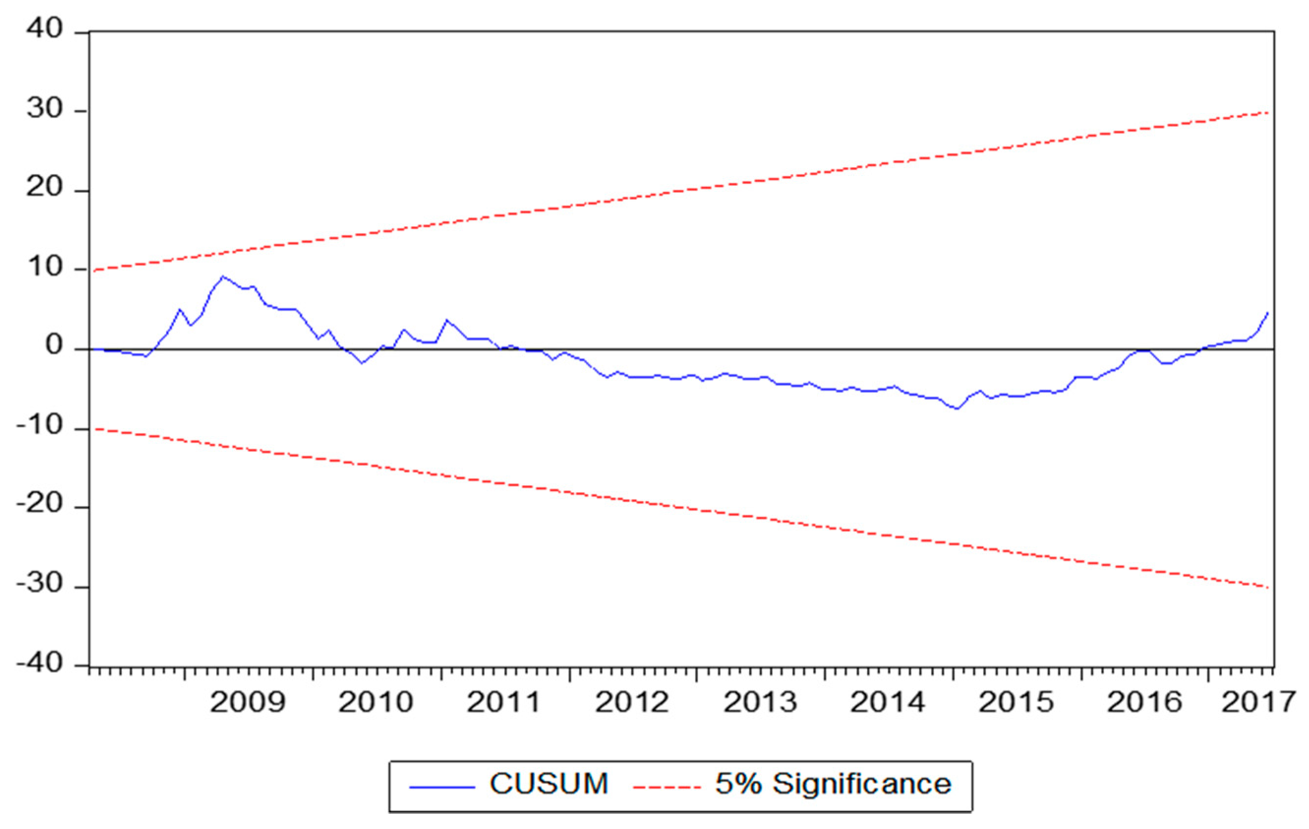
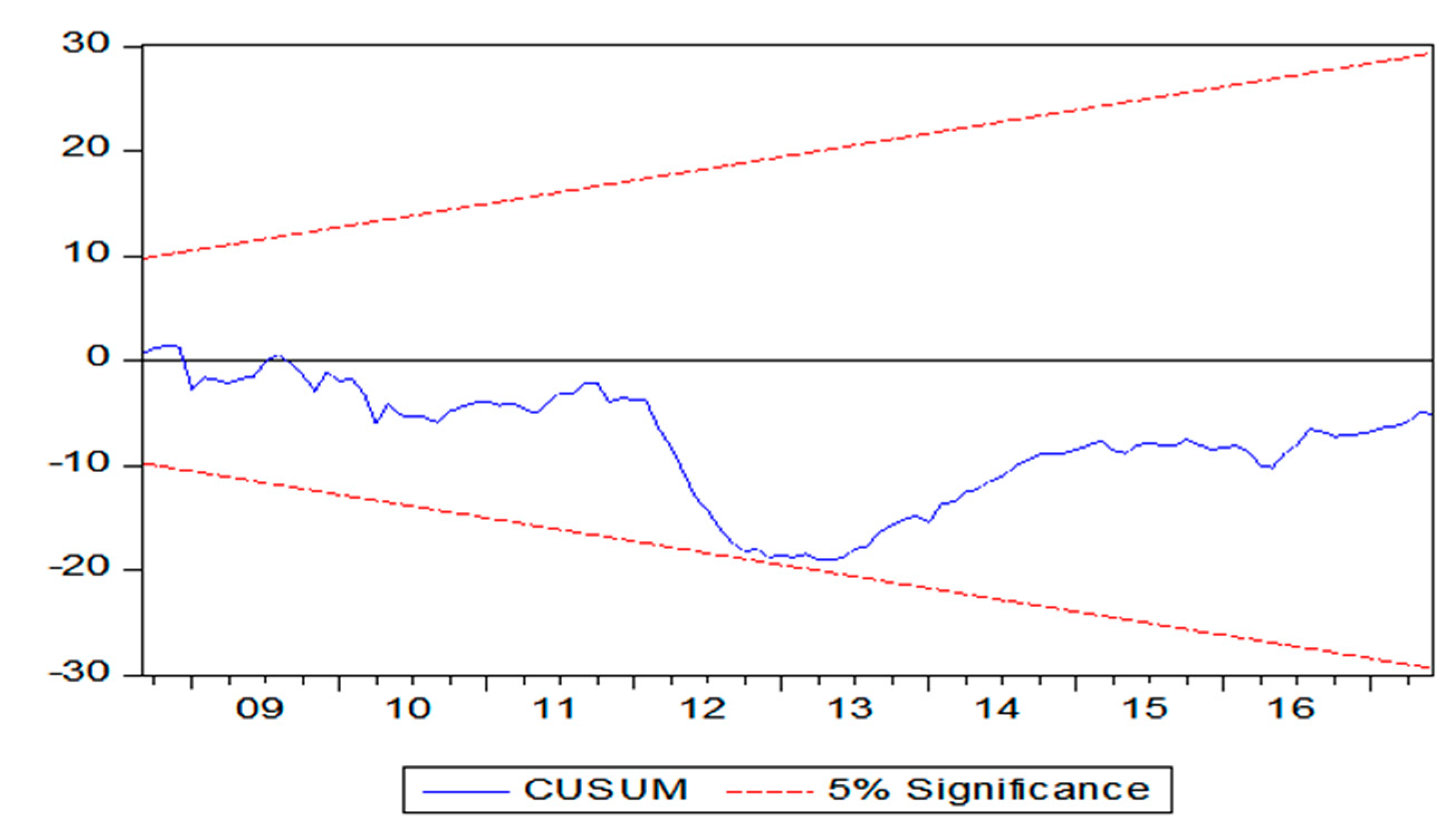
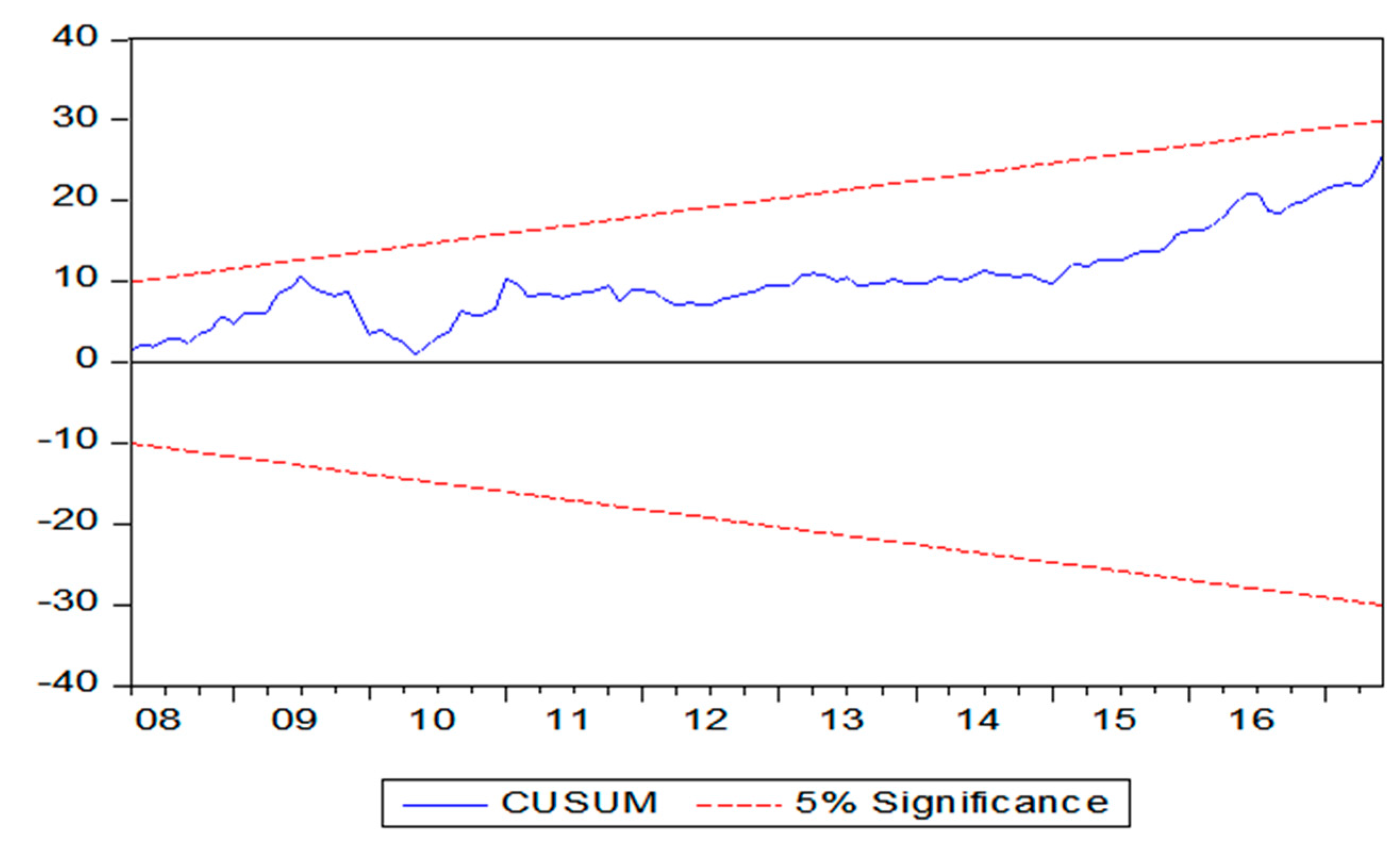
Nevertheless, for both farm-wholesale and retail-wholesale prices, the presence of asymmetry can’t be denied according to the asymmetry error correction model result presented which is also in line with the earlier study [5] regarding price transmission issue along the vertical supply chain of rice in Bangladesh. These findings provide evidence to the long-held common perception of the consumers, producers as well as the government about probable market manipulation or inefficiency. To some extent presence of asymmetry may not be concluded firmly because in our ECM we are confined to capture asymmetry only by considering zero thresholds which may not be the most appropriate value in the case of modern distribution practice. Therefore, this limitation has been taken into consideration and an approach has been made in the next step to find out the possible threshold which affects the degree or speed of asymmetry among the market pairs. LM and ARCH tests based on the respective number of lags are conducted as diagnostics tests for both price pairs. The results indicate that the estimated models for both farm-wholesale and retail-wholesale price pairs are free from serial correlation and heteroscedasticity. Then, model stability was tested by CUSUM test which suggests that models are stable for both pairs as the estimated lines for both models lie between the 5% level significance line (Appendix A: Figure A1 and Figure A2).
3.5. Non-Linear Price Transmission Analysis by TAR and M-TAR Model
Table 7 represents the results of the threshold autoregressive and momentum threshold autoregressive model for both the marketing pair along the vertical supply chain of rice namely, farm-wholesale and retail-wholesale prices.
The results of TAR-ECM and MTAR-ECM models are shown in Table 6 where the optimal threshold values are estimated first by minimizing the sum of the residuals squares.
It is to be noted that, the number of lags included in TAR and M-TAR models are selected based on AIC and SBIC. Lag 4 and 1 are selected as optimal lag for farm-wholesale and retail-wholesale prices, respectively. According to the threshold co-integration test based on the TAR model reported in Table 6, rejects the null hypothesis of no threshold cointegration at 5% level of significance for both farm-wholesale and retail-wholesale price pairs. Again, rejects the null hypothesis of no threshold co-integration at 1% and 5% level of significance for both farm-wholesale and retail-wholesale price pairs, respectively, in case of threshold co-integration test based on M-TAR model as well. So, as the null hypothesis of no co-integration is rejected for both market pairs at 1% or 5% level of significance for both TAR and M-TAR models and the sign of all coefficients are also negative which is a necessary condition for long-run convergence, it is evident that both market pairs are converged to equilibrium in the long-run i.e., prices of both markets may deviate in short-run but they are being adjusted to equilibrium in long-run.
Given that the series are co-integrated, analysis is being headed to test the null hypothesis of symmetric adjustment ( using a standard F-distribution. In the case of farm-wholesale price pair, about 26% of a positive deviation and 15% of a negative deviation from the long-run equilibrium relationship are eliminated within a month where the null of symmetry can’t be rejected as the F-statistics is not significant. But F-statistics for M-TAR model gives significant result at 5% level of significance where more discrepancy is observed in adjustment between positive and negative deviation which lead us to reject the null of symmetry in that case. Our result from M-TAR indicates that about 53% and 88% of positive and negative discrepancies from the equilibrium, respectively, would still persist in the following months. On the other hand, In case of retail-wholesale price pair TAR model indicates that about 11% of a positive deviation and 26% of a negative deviation from the long-run equilibrium relationship are eliminated within a month where the null of symmetry can be rejected as the F-statistics is significant at 10% level of significance. In other words, we can say that about 89% of positive and 74% of negative divergences from the equilibrium would still linger in the following months.
Since both the TAR and M-TAR models reveal asymmetric adjustment for all the series of both market pairs, it would be interesting to ascertain whether adjustment follows a TAR or M-TAR process. For such a test, Enders & Siklos [30] suggest using the SBIC or AIC test values to select the model with the best overall fit. As is evident in Table 5, the M-TAR model yields the lowest SBIC and AIC and is therefore preferable to the TAR model for explaining the asymmetric adjustment of upstream prices i.e., farm-wholesale price pair. TAR model yields the lowest SBIC and AIC for retail-wholesale market pairs and thus, it was preferable to M-TAR model. Ljung-box Q-statistics up to 4 and 8 lags and ARCH tests are conducted as diagnostics tests. The results indicate that the estimated models (TAR and M-TAR) for both farm-wholesale and retail-wholesale price pairs are free from serial correlation and heteroscedasticity. At the end, stability was tested by the CUSUM test for each TAR and M-TAR model which suggests that all models are stable except the M-TAR model for retail-wholesale price pair (Appendix A: Figure A3 and Figure A4)
It is therefore concluded that there are threshold effects on the co-integration of markets along the vertical supply chain of rice in Bangladesh. Results fromTAR & M-TAR indicating the presence of one or multiple factors that may affect the price transmission in the long-run. Previous literature [34] observing the same mentioned large transaction cost, policy interventions etc. as the threshold factor in developing countries. But in the case of Bangladesh’s rice market, it requires another investigation as the scope of this paper only allows us to evident the presence of asymmetry rather than causes. Both upstream (farm-wholesale) and downstream (retail-wholesale) markets show a significant asymmetry in price transmission where the upstream market responds more swiftly to price decrease than to price increase and downstream markets just do the opposite as it responds more quickly to a price increase than to decrease and all these adjustment process varies based on some threshold values which reveals the requirement of some effective policies to eliminate these irregularities.
3.6. Limitations
Several reasons are acknowledged in the literature to explain the causes of asymmetric price transmission in the spatial and vertical food markets. Potential explanations for the asymmetric price transmission are retail level market power [35,36,37], adjustment costs [38,39], search costs [28,40], inventory holding management costs [41,42], asymmetric information [43,44], market structure [45], public intervention [46]. Although it is widely discussed in the literature that market power is the main cause for imperfect price transmission especially at the retail level but in many cases, it may not be true at all especially in developing countries where numerous actors are present in these markets. However, presence of threshold effect on price transmission also gives us evidence about the urgency of effective policy interventions in rice supply chain. In Bangladesh, domestic rice markets are mainly driven by millers and wholesalers. The wholesalers purchase rice from the millers. The millers and wholesalers are not too many in numbers who have a great turnover in the market because of their high handling capacity and huge investment. Therefore, it is very much likely that millers and wholesalers could manipulate market prices through collusion. However, the scope of this paper does not allow us to test if millers and wholesalers are responsible for this price asymmetry.
4. Conclusions
Rice markets in Bangladesh are characterized by private and public existence. Domestic and border policies are liberalized allowing the private traders to involve in rice markets. The government of Bangladesh procures paddy from farmers by paying them support price which is set higher than the market price. The government also procures rice from rice processors or millers every year. However, the quantity of procurement from farmers and millers is very insignificant. Public import and food aid or other social safety programs constitute a small percent of the total supply. Due to liberal market policies and less public intervention, numerous private traders are involved from rice production and marketing until the end-users. This, in turn, creates a great concern that markets are not efficient to ensure maximum welfare for both the consumers and producers which is evident from our study results also as short-run and long-run asymmetry were found for both upstream and downstream markets. A negative deviation is found to be more persistent than a positive one in the case of upstream market pair by which farmers or producers are often being the sufferer as a decrease of the price is being prevailed for a longer time. On the other hand, more persistence of positive deviation than the negative deviation from long-run equilibria in the case of downstream market pair was found which affects the end consumers a lot as an increase in price is being prevailed for a long time which is also in line with industrial organization theory. This also validates the hypothesis of the ‘rocket and feather’ principle in the vertical rice markets in Bangladesh which affects the welfare inversely as producers are not being able to get the benefit from price level rise in retail level while end consumers are also not being able to capture the benefit of price fall in producer level. Furthermore, existence of shocks or threshold effects in price transmission indicates the urgency of policy interventions in the domestic rice market to ensure maximum welfare both for producers and consumers.
However, as the study results have found the wholesale price to lead farm and retail prices in the case of upstream and downstream markets, respectively; that attract attention to the effective policy implications by targeting wholesale level. Even though the overall rice markets are well integrated but due to the existence of positive and negative asymmetry mainly driven by the wholesale level, processors and wholesalers should have brought under some regulations by introducing a comprehensive trade policy to refrain them from probable manipulation of the market. In that case, market infrastructures should be developed more by increasing public interventions. Introduction of rice processing centers, central wholesale markets etc. could be the probable solutions that are now absent in the country’s context Farmer’s associations or cooperatives need to be introduced to balance the market power and reduce information asymmetry as well. It is high time to formulate a well-directed and executable price policy in the rice market which is surprisingly absent yet in the case of Bangladesh. Above all, this study raises the concern of making more advanced research by using the state-of-art methodology to find out the exact causes behind market inefficiency like asymmetry in price transmission and to ensure better policy directions.
Author Contributions
L.D. made the formal analysis and wrote the paper; Y.L. helped in conceptualization and was involved in review process, S.H.L. reviewed the paper and supervised the overall research as well. All authors have read and agreed to the published version of the manuscript.
Funding
This research received no external funding.
Acknowledgments
This paper is a modified version of Limon Deb’s master thesis completed at Kangwon National University.
Conflicts of Interest
The authors declare no conflict of interest.
Appendix A

Table A1.
Selection of Optimum Lag Length for Farm, wholesale and Retail prices in Johansen Co-integration Test.
Table A1.
Selection of Optimum Lag Length for Farm, wholesale and Retail prices in Johansen Co-integration Test.
| Lag | LR | FPE | AIC | SC | HQ |
|---|---|---|---|---|---|
| 0 | NA | 7.64 × 10⁻⁷ | −5.571373 | −5.501686 | −5.543073 |
| 1 | 656.5394 | 3.09/109 | −11.08120 | −10.80245 * | −10.96799 * |
| 2 | 17.56566 * | 3.08/109 * | −11.08664 * | −10.59883 | −10.88854 |
| 3 | 8.773931 | 3.30/109 | −11.01641 | −10.31953 | −10.73340 |
| 4 | 16.78309 | 3.28/109 | −11.02326 | −10.11732 | −10.65535 |
Note: * is the optimum lag length.
Table A2.
Selection of Optimum Lag Length for Farm-Wholesale Price Pair.
| Lag | LR | FPE | AIC | SC | HQ |
|---|---|---|---|---|---|
| 0 | NA | 0.000223 | −2.734494 | −2.688036 | −2.715628 |
| 1 | 441.6655 | 5.46/106 | −6.442747 | −6.303372 | −6.386146 |
| 2 | 18.53178 | 4.97/106 | −6.537226 | −6.304935 * | −6.442892 * |
| 3 | 8.256243 | 4.94/106 | −6.543623 | −6.218416 | −6.411555 |
| 4 | 11.18582 * | 4.77/106 * | −6.577730 * | −6.159606 | −6.407928 |
| 5 | 1.672779 | 5.02/106 | −6.526410 | −6.015370 | −6.318874 |
| 6 | 1.089080 | 5.32/106 | −6.469922 | −5.865965 | −6.224652 |
| 7 | 0.407322 | 5.67/106 | −6.407134 | −5.710261 | −6.124131 |
| 8 | 1.327303 | 5.99/106 | −6.353354 | −5.563565 | −6.032617 |
Note: * is the optimum lag length.
Table A3.
Selection of Optimum Lag Length for Retail-Wholesale Price Pair.
| Lag | LR | FPE | AIC | SC | HQ |
|---|---|---|---|---|---|
| 0 | NA | 8.78/105 | −3.665167 | −3.618708 | −3.646300 |
| 1 | 503.3772 * | 1.27/106 * | −7.900869* | −7.761495 * | −7.844268 * |
| 2 | 3.055629 | 1.32/106 | −7.860773 | −7.628482 | −7.766439 |
| 3 | 1.714242 | 1.39/106 | −7.809277 | −7.484069 | −7.677209 |
| 4 | 6.444439 | 1.40/106 | −7.800668 | −7.382544 | −7.630866 |
| 5 | 7.486049 | 1.40/106 | −7.802681 | −7.291641 | −7.595145 |
| 6 | 5.268256 | 1.43/106 | −7.785250 | −7.181294 | −7.539981 |
| 7 | 3.203863 | 1.48/106 | −7.749096 | −7.052224 | −7.466093 |
| 8 | 4.207150 | 1.52/106 | −7.723276 | −6.933487 | −7.402539 |
Note: * is the optimum lag length.
Figure A1.
CUSUM Test Result of Asymmetric Error Correction Model (Farm-Wholesale).

Figure A2.
CUSUM Test Result of Asymmetric Error Correction Model (Retail-Wholesale).

Figure A3.
CUSUM Test Result of M-TAR Model (Farm-Wholesale).
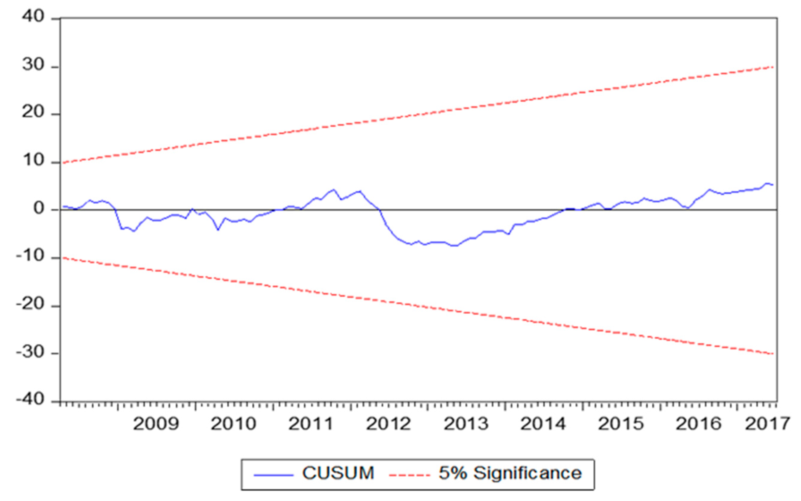
Figure A4.
CUSUM Test Result of TAR Model (Retail-Wholesale).
References
- Conforti, P. Price transmission in selected agricultural markets. In FAO Commodity and Trade Policy Research Working Paper No. 7; Food and Agriculture Organization (FAO): Rome, Italy, 2004. [Google Scholar]
- Asche, F.; Jaffry, S.; Hartmann, J. Price transmission and market integration: Vertical and horizontal price linkages for salmon. Appl. Econ. 2007, 39, 2535–2545. [Google Scholar] [CrossRef]
- Mottaleb, K.A.; Mishra, A.K. Rice consumption and grain-type preference by household: A Bangladesh case. J. Agric. Appl. Econ. 2016, 48, 298–319. [Google Scholar] [CrossRef] [Green Version]
- United States Department of Agriculture (USDA). Production, Import, Supply and Distribution Online Database; Foreign Agriculture Service; United States Department of Agriculture: Washington, DC, USA, 2019. Available online: https://apps.fas.usda.gov/psdonline (accessed on 4 August 2019).
- Alam, M.J.; McKenzie, A.M.; Buysse, J.; Begum, I.A.; Wailes, E.J.; Van Huylenbroeck, G. Asymmetry Price Transmission in the Deregulated Rice Markets in Bangladesh: Asymmetric Error Correction Model. Agribusiness 2016, 32, 498–511. [Google Scholar] [CrossRef]
- Zaki-Uz, Z.; Mishima, T.; Hisano, S.; Gergely, M.C. The Role of Rice Processing Industries in Bangladesh: A Case Study of Sherpur District. Hokkaido Univ. Agric. Econ. 2001, 57, 121–133. [Google Scholar]
- Goletti, F.A.; Farid, N.R. Structural determinants of rice market integration: The case of rice markets in Bangladesh. Dev. Econ. 1995, 33, 185–202. [Google Scholar] [CrossRef]
- Dawson, P.J.; Dey, P.K. Testing for the law of one price: Rice market integration in Bangladesh. J. Int. Dev. 2002, 14, 473–484. [Google Scholar] [CrossRef]
- Engle, R.F.; Granger, C.W.J. Co-integration and Error Correction: Representation, Estimation, and Testing. Econometrica 1987, 55, 251–276. [Google Scholar] [CrossRef]
- Johansen, S. Statistical analysis of cointegration vectors. J. Econ. Dyn. Control 1988, 12, 231–254. [Google Scholar] [CrossRef]
- Johansen, S. Estimation and Hypothesis Testing of Cointegration Vectors in Gaussian Vector Autoregressive Models. Econom. J. Econom. Soc. 1991, 1551–1580. [Google Scholar] [CrossRef]
- Dickey, D.; Fuller, W. Distribution of the estimators for autoregressive time series with a unit root. J. Am. Stat. Assoc. 1979, 74, 427–431. [Google Scholar]
- Ng, S.; Perron, P. Unit Root Tests in ARMA Models with Data-Dependent Methods for the Selection of the Truncation Lag. J. Am. Stat. Assoc. 1995, 90, 268–281. [Google Scholar] [CrossRef]
- Newey, W.; Kenneth, W. Automatic lag selection in covariance matrix estimation. Rev. Econ. Stud. 1994, 61, 631–653. [Google Scholar] [CrossRef]
- Gujarati, D.N. Basic Econometrics; Tata McGraw-Hill Education: New Delhi, India, 2009. [Google Scholar]
- Mosconi, R.; Giannini, C. Non-causality in cointegrated systems: Representation, estimation and testing. Oxf. Bull. Econ. Stat. 1992, 54, 399–417. [Google Scholar] [CrossRef]
- Dolado, J.; Lutkepohl, H. Making Wald tests for cointegrated VAR systems. Econom. Rev. 1996, 15, 369–386. [Google Scholar] [CrossRef]
- Houck, J.P. Nonreversible and Estimating an Approach to Specifying Functions. Am. J. Agric. Econ. 1977, 59, 570–572. [Google Scholar] [CrossRef]
- Mohanty, S.; Peterson, E.W.F.; Kruse, N.C. Price asymmetry in the international wheat market. Can. J. Agric. Econ. 1995, 43, 355–366. [Google Scholar] [CrossRef]
- Peltzman, S. Prices Rise Faster than They Fall. J. Political Econ. 2000, 108, 466–502. [Google Scholar] [CrossRef]
- Bart, M.; Steven, K. Retail margins, price transmission and price asymmetry in urban food markets: The case of Kinshasa (Zaire). J. Afr. Econ. 2000, 9, 1–23. [Google Scholar]
- Aguiar, D.; Santana, J.A. Asymmetry in farm to retail price transmission: Evidence for Brazil. Agribusiness 2002, 18, 37–48. [Google Scholar] [CrossRef]
- Von Cramon-Taubadel, S.; Loy, J.P. Price asymmetry in the international wheat market: Comment. Can. J. Agric. Econ. 1996, 44, 311–317. [Google Scholar] [CrossRef]
- Von Cramon-taubadel, S. Estimating asymmetric price transmission with the error correction representation: An application to the German pork market. Eur. Rev. Agric. Econ. 1998, 25, 1–18. [Google Scholar] [CrossRef]
- Abdulai, A. Spatial price transmission and asymmetry in the Ghanaian maize market. J. Dev. Econ. 2000, 63, 327–349. [Google Scholar] [CrossRef]
- Michela, C.; Kirsten, J. Asymmetric price transmission and market concentration: An investigation into four South African agro-food industries. S. Afr. J. Econ. 2006, 74, 323–333. [Google Scholar]
- Van, C. Modeling trends in food market integration: Method and application to Tanzanian maize markets. Food Policy 2007, 32, 112–127. [Google Scholar]
- Gomez, M.I.; Richards, T.J.; Lee, J. Trade promotions and consumer search in supermarket retailing. Am. J. Agric. Econ. 2013, 95, 1209–1215. [Google Scholar] [CrossRef]
- Kuiper, W.E.; Lutz, C.; Van Tilburg, A. Vertical price leadership on local maize markets in Benin. J. Dev. Econ. 2003, 71, 417–433. [Google Scholar] [CrossRef] [Green Version]
- Enders, W.; Siklos, P.L. Cointegration and Threshold Adjustment. J. Bus. Econ. Stat. 2001, 19, 166–167. [Google Scholar] [CrossRef] [Green Version]
- Ndoricimpa, A.; Achandi, L.E. Are current account deficits sustainable in EAC countries? Evidence from Threshold Cointegration. Econ. Bull. 2014, 34, 1990–2001. [Google Scholar]
- Chan, K.S. Consistency and Limiting Distribution of the Least Squares Estimator of a Threshold Autoregressive Model. Ann. Stat. 1993, 21, 520–533. [Google Scholar] [CrossRef]
- Acquah, H.D. Threshold Cointegration Analysis of Asymmetric Adjustments. Russ. J. Agric. Socio-Econ. Sci. 2012, 8, 21–25. [Google Scholar]
- Alam, M.J.; Jha, R. Asymmetric threshold vertical price transmission in wheat and flour markets in Dhaka (Bangladesh): Seemingly unrelated regression analysis. In ASARC Working Papers; The Australian National University, Australia South Asia Research Centre: Canberra, Australia, 2016. [Google Scholar]
- Griffith, G.R.; Piggott, N. Asymmetry in Beef, Lamb and Pork Farm-Retail Price Transmission in Australia. Agric. Econ. 1994, 10, 307–316. [Google Scholar]
- Bettendorf, L.; Verboven, F. Incomplete transmission of coffee bean prices: Evidence from the Dutch coffee market. Eur. Rev. Agric. Econ. 2000, 27, 1–16. [Google Scholar] [CrossRef]
- Moorthy, S. A general theory of pass-through in channels with category management and retail competition. Mark. Sci. 2005, 24, 110–122. [Google Scholar] [CrossRef]
- Buckle, R.A.; Carlson, J.A. Inflation and asymmetric price adjustment. Rev. Econ. Stat. 2000, 82, 157–160. [Google Scholar] [CrossRef]
- Chavas, J.P.; Mehta, A. Price Dynamics in a Vertical Sector: The Case of Butter. Am. J. Agric. Econ. 2004, 86, 1078–1093. [Google Scholar] [CrossRef] [Green Version]
- Richards, T.J.; Gomez, M.I.; Lee, J. Pass-through and consumer search: An empirical analysis. Am. J. Agric. Econ. 2014, 96, 1049–1069. [Google Scholar] [CrossRef] [Green Version]
- Reagan, P.B.; Weitzman, M.L. Asymmetries in price and quantity adjustments by the competitive firm. J. Econ. Theory 1982, 27, 410–420. [Google Scholar] [CrossRef]
- Cui, T.H.; Raju, J.S.; Zhang, Z.J. A price discrimination model of trade promotion. Mark. Sci. 2008, 27, 779–795. [Google Scholar] [CrossRef] [Green Version]
- Bailey, D.; Brorsen, B.W. Price Asymmetry in Spatial Fed Cattle Markets. West. J. Agric. Econ. 1989, 14, 246–252. [Google Scholar]
- Kumar, N.; Rajiv, S.; Jeuland, A. Effectiveness of trade promotions: Analyzing the determinants of retail pass through. Mark. Sci. 2001, 20, 382–404. [Google Scholar] [CrossRef] [Green Version]
- Lee, J.; Gomez, M.I. Impacts of the end of the coffee export quota system on international-to-retail price transmission. J. Agric. Econ. 2013, 64, 343–362. [Google Scholar] [CrossRef] [Green Version]
- Kinnucan, H.W.; Forker, O.D. Asymmetry in farm-retail price transmission for major dairy products. Am. J. Agric. Econ. 1987, 69, 285–292. [Google Scholar] [CrossRef]

Figure 2.
Evolution of farm, wholesale and retail prices of rice from November 2006 to June 2017.

Table 1.
Summary of hypotheses and decision rules of causality test.
| Sources of Causations | Hypotheses | Price Leadership Decisions | Causality Decisions |
|---|---|---|---|
| Long-run causality | No price leadership | Bidirectional | |
| Farm leads Wholesale Retail leads Wholesale | Unidirectional | ||
| Wholesale leads Farm Wholesale leads Retail | Unidirectional | ||
| Short-run causality | No price leadership | Bidirectional | |
| Farm leads Wholesale Retail leads Wholesale | Unidirectional | ||
| Wholesale leads Farm Wholesale leads Retail | Unidirectional | ||
| Strong exogeneity | No price leadership | Bidirectional | |
| Farm leads Wholesale Retail leads Wholesale | Unidirectional | ||
| Wholesale leads Farm Wholesale leads Retail | Unidirectional |
Table 2.
Stationarity Test Result.
| Price Series/Tests | Level Data | First Differences | Order of Integration | |||
|---|---|---|---|---|---|---|
| γ-statc | γ-statc,t | γ-statw | I(d) | |||
| Farm Price (FP) | ||||||
| ADF | −2.68 | −3.70 | −8.11 *** | I(1) | ||
| PP | −2.47 | −2.91 | −8.17 *** | |||
| Wholesale Price (WP) | ||||||
| ADF | −2.65 | −3.38 | −9.31 *** | I(1) | ||
| PP | −2.24 | −2.69 | −9.69*** | |||
| Retail Price (RP) | ||||||
| ADF | −2.57 | −3.89 | −9.37 *** | I(1) | ||
| PP | −2.55 | −2.97 | −9.94 *** | |||
| Critical Values | γ-statc | γ-statc,t | γ-statw | |||
| Level of Significance | 1% | 5% | 1% | 5% | 1% | 5% |
| ADF | −3.48 | −2.88 | −4.03 | −3.45 | −2.58 | −1.94 |
| PP | −3.48 | −2.88 | −4.03 | −3.45 | −2.58 | −1.94 |
Note: Lag length for ADF test is decided based on Akaike info criteria (AIC); maximum bandwidth for PP test is decided based on Newey-West (1994); ∗∗∗ indicates that unit root in the first differences are rejected at 1% level; γ-statc, γ-statc,t and γ-statw indicate τ-statistics of random walk with constant only, constant and trend, and pure random walk or no constant and trend models, respectively.
Table 3.
Johansen Test for Co-integration.
| Retail, Wholesale and Farm Level | ||||
|---|---|---|---|---|
| Co-Integration Rank (r) | ||||
| r = 0 vs. | 41.94848 *** | 29.79707 | 21.23827 ** | 21.13162 |
| r ≤ 1 vs. | 20.71021 *** | 15.49471 | 14.12689 * | 14.26460 |
| r ≤ 2 vs. | 6.583319 ** | 3.841466 | 6.583319 ** | 3.841466 |
Note: ***, ** and * indicate the hypothesis is rejected at 1%, 5% and 10% significance level, respectively.
Table 4.
Restriction on the Johansen VECM for testing Causality between Farm and Wholesale price.
| Causality Test | |||
|---|---|---|---|
| Sources of Causations | Dependent Variable ∆FP | Dependent Variable ∆WP | Causality Decision |
| Long-run causality | vs. 7.196448 ** [0.0073] | vs. 0.895 [0.3442] | Unidirectional (Wholesale → Farm) |
| Short-run causality | vs. 5.64240 [0.1304] | vs. 10.12207 ** [0.0176] | Unidirectional (Farm → Wholesale) |
| Strong exogeneity | vs. 15.30817 ** [0.0041] | vs. 20.10853 ** [0.0005] | Bidirectional (Wholesale ⬌ Farm) |
Note: ** Indicates the significance level at 5%; probability levels are in the parentheses.
Table 5.
Restriction on the Johansen VECM for testing Causality between Retail and Wholesale price.
| Causality Test | |||
|---|---|---|---|
| Sources of Causations | Dependent Variable ∆RP | Dependent Variable ∆WP | Causality Decision |
| Long-run causality | vs. 11.24899 ** [0.0008] | vs. 0.512 [0.4743] | Unidirectional (Wholesale → Retail) |
| Short-run causality | vs. 2.621539 * [0.0954] | vs. 0.1277 [0.7207] | Unidirectional (Wholesale → Retail) |
| Strong exogeneity | vs. 17.61459 ** [0.0041] | vs. 0.627841 [0.7306] | Unidirectional (Wholesale → Retail) |
Note: ** and * Indicate the significance level at 5% and 10%, respectively; probability levels are in the parentheses.
Table 6.
Results of the Asymmetric Error Correction Model.
| Farm-Wholesale | Retail-Wholesale | ||||
|---|---|---|---|---|---|
| Regressors | Coefficients | t-Statistics | Regressors | Coefficients | t-Statistics |
| 0.288555 ** | 2.891544 | −0.132748 | −1.504456 | ||
| 0.025737 | 0.246374 | 0.583457 *** | 8.474050 | ||
| −0.008676 | −0.079020 | 0.139843 * | 1.884684 | ||
| 0.061633 | 0.558938 | 0.089580 | 1.086427 | ||
| 0.505198 ** | 3.387956 | 0.068034 | 0.737192 | ||
| 0.218602 | 0.984663 | ||||
| 0.003069 | 0.018612 | ||||
| 0.009870 | 0.043138 | ||||
| 0.085525 | 0.512652 | ||||
| −0.076931 | −0.360297 | ||||
| 0.213523 * | 1.692238 | ||||
| 0.187891 | 0.916896 | ||||
| −0.038645 | −0.242151 | ||||
| −0.048874 | −0.254390 | ||||
| −0.299727 * | −1.892067 | −0.106754 ** | −2.558078 | ||
| −0.157633 * | −1.932706 | −0.181382 ** | −2.200916 | ||
| LM test ARCH test Normality test (Jarque-Bera) CUSUM test | 0.8235 [~F (4,102)] 0.9998 [~F (4,114)] 2.30 [0.102] S | 0.3524 [~F (1,117)] 0.5831 [~F (1,123)] 2.58 [0.112] S | |||
| Farm-Wholesale | Retail-Wholesale | ||||
| Test of co-integration (from asymmetric model) | |||||
(No Co-integration) | (0.009 ***) | (No co-integration) | (0.0002 ***) | ||
| Wald test for symmetry | |||||
| Hypothesis 1 | (0.096 *) | Hypothesis 1 | (0.151) | ||
| Hypothesis 2 | F-stat: 2.227 (0.089 *) | Hypothesis 2 | F-stat: 6.269 (0.002 ***) | ||
Note: ***, **, and * indicate that the hypotheses are rejected at 1%, 5% and 10% level of significance, respectively, parentheses are presenting probability level, LM and ARCH test mean Breusch-Godfrey Serial Correlation LM test and Autoregressive Conditional Heteroscedasticity test, respectively; CUSUM is the stability test for the model where S depicts that the model satisfied the test.
Table 7.
Threshold Co-integration Test Results with the TAR and M-TAR model.
| Market Pairs | Farm-Wholesale | Retail-Wholesale | ||
|---|---|---|---|---|
| TAR | M-TAR | TAR | M-TAR | |
| −0.263102 ** (0.115) | −0.125598 ** (0.062) | −0.110574 ** (0.041) | −0.135571 ** (0.039) | |
| −0.151137 ** (0.077) | −0.475233 *** (0.114) | −0.263558 ** (0.066) | −-0.099894 (0.065) | |
| 10.50063 ** | 19.04142 *** | 14.32855 ** | 14.08717 ** | |
| F-statistics | 0.581604 | 8.425138 ** | 3.429578 * | 0.213173 |
| -0.068218 | −0.032160 | −0.051041 | −0.015185 | |
| AIC | −3.161186 | −3.229120 | −4.613962 | −4.552164 |
| SBIC | −2.886827 | −2.954760 | −4.478901 | −4.407103 |
| LB (4) | 0.999 | 0.997 | 0.333 | 0.389 |
| LB (8) | 0.505 | 0.994 | 0.122 | 0.146 |
| Lags | 4 | 4 | 1 | 1 |
Note: λ is the estimated threshold value. Between the parentheses (.) are the standard errors. *, ** and *** denote rejection of the null hypothesis respectively at10%, 5% and 1% level, respectively. Φ is the threshold co-integration test statistic. F-statistic is the test for symmetry adjustment. The values presented for Ljung-Box (LB) test are the p-values. The lag length used was selected using AIC and SBIC.
© 2020 by the authors. Licensee MDPI, Basel, Switzerland. This article is an open access article distributed under the terms and conditions of the Creative Commons Attribution (CC BY) license (http://creativecommons.org/licenses/by/4.0/).
Share and Cite
MDPI and ACS Style
Deb, L.; Lee, Y.; Lee, S.H. Market Integration and Price Transmission in the Vertical Supply Chain of Rice: An Evidence from Bangladesh. Agriculture 2020, 10, 271. https://doi.org/10.3390/agriculture10070271
AMA Style
Deb L, Lee Y, Lee SH. Market Integration and Price Transmission in the Vertical Supply Chain of Rice: An Evidence from Bangladesh. Agriculture. 2020; 10(7):271. https://doi.org/10.3390/agriculture10070271
Chicago/Turabian StyleDeb, Limon, Yoonsuk Lee, and Sang Hyeon Lee. 2020. "Market Integration and Price Transmission in the Vertical Supply Chain of Rice: An Evidence from Bangladesh" Agriculture 10, no. 7: 271. https://doi.org/10.3390/agriculture10070271
Note that from the first issue of 2016, this journal uses article numbers instead of page numbers. See further details here.