Evaluating Alternative Methods of Soil Erodibility Mapping in the Mediterranean Island of Crete

Abstract

Soil erodibility is among the trickiest erosion factors to estimate. This is especially true for heterogeneous Mediterranean environments, where reliable and dense soil data are rarely available, and interpolation methods give very low accuracies. Towards estimating soil erodibility, research so far has resulted in several alternatives mainly based on empirical formulas, on physics-based equations or on inference with expertise. The aim of this work was to compare erodibility patterns derived by using the empirical United States Department of Agriculture (USDA) formula and by inference from a geological map in a Mediterranean agricultural site. The Kolymvari area, located in the western part of Crete, an area covered by olive groves and citrus orchards, was selected as the study site for this work. Comparison of the spatial patterns of soil erodibility derived from the two alternatives showed significant differences (i.e., a mean normalized difference value of 0.52), while a test of the “inference” alternative indicated very low accuracies (0.1475 RMS error). A comparison, however, of the spatial patterns of erosion values derived from both alternatives indicated that dissimilarities of the two soil erodibility maps faded out. Moreover, the highly risky areas provided by both alternatives were found to be identical for 88% of the whole study site.

1. Introduction

Soil erosion is the process of detachment and transport of soil materials by wind or water [1]. In erosion caused by water, raindrops falling on bare soil break down the structure of the surface soil and detach particles. If the land is sloping and the water cannot be immediately absorbed by the soil or detained by the microtopography, the water moves off down the slope in the form of run-off, carrying dislodged particles with it [2]. The inherent trend of a soil to be eroded is defined as soil erodibility (or K-factor, as inherited from universal soil loss equation (USLE) literature) and is influenced by infiltration rate, permeability, surface sealing, structure, texture, organic matter content, surface gravel, total water capacity, etc. [3]. Sanders [2] discriminates erodibility into detachability and transportability. A complete overview of erosion physics and terminology can be found in [3,4,5,6].

Mediterranean regions are extremely prone to erosion by water. Dry summer periods frequently coincide with violent rainstorms, causing very high yearly soil losses [7]. Inappropriate land use practices contribute to the acceleration of these degradation processes, as large areas suffer from overgrazing and overexploitation of water resources by agriculture and tourism [8]. Excess human pressure on natural resources appears to coincide with more frequent high intensity rainfall potentials in the 21st century, rendering the allocation of regions at risk of severe degradation (called “hot spots”) an urgent task for land use planners and decision makers in the Mediterranean [9].

This emergency has been recognized by many national and international authorities; for example, the European Union (EU) has addressed soil erosion as one of the most hazardous soil degradation parameters [10]. The main expectation from this kind of policy is to control and finally ensure the effectiveness of protection measures against soil erosion, by comprehensive monitoring [11]. In this direction, information about current erosion patterns, erosion risk and future trends can be provided by effective soil erosion modeling, which, moreover, can allow scenario analysis in relation to current or alternative land uses [12].

Soil erosion models can be distinguished in two major categories [2,13]: (a) empirical (or statistical or regression) models, which estimate erosion results based on regression of soil loss with land physical properties and climate characteristics (e.g., USLE, Erosion Productivity Index Calculator-EPIC, Coordinate Information on the Environment-CORINE, Gavrilovic, etc.); and (b) mechanistic (or process-based or physics-based) models, which simulate the physical erosion processes by resolving the fundamental physical equations that describe stream flow and sediment generation (e.g., Topographic Model-TOPMODEL, Areal Nonpoint Source Watershed Environmental Response Simulation-ANSWERS, Chemicals, Runoff and Erosion from Agricultural Management Systems-CREAMS, Water Erosion Prediction Process-WEPP, MEDALUS Desertification Response Unit SHE-MEDRUSH, where MEDALUS stands for Mediterranean Desertification and Land Use impacts and SHE stands for Système Hydrologique Européen, Pan European Soil Erosion Risk Assessment-PESERA, etc.) [14].

When implementation of an erosion model is concerned, users have to do specific choices about the input datasets and processing techniques, depending on their expertise, local conditions and data availability and appropriateness. As a general rule, there is no optimal model nor optimal data, but a correlation between the quality of input data and the optimal complexity of the model [15]. Using a big set of pits under a mildly Mediterranean climate (close to Madrid), [16] concluded that input data for the K-factor used in the USLE formula [3] should not be derived from a soil map unless a key soil factor could be identified. Alternatively, they suggested use of physiographic instead of soil maps. The process of matching data with model requirements could be considered as a kind of model calibration.

In addition to that, modeling performance and results can be seen from two different points of view: the view of researchers and the view of decision makers. Researchers are focused mainly on the precise performance of a model and are more concerned with simulating what has occurred than with predicting future events. Policy makers, on the other hand, intend to use models in the framework of natural resource management and land use planning on large scales in a legal and social context, and therefore, they focus on predictions or risk of future events [17]. In these cases, adequate and appropriate soil data are rarely available and expensive to obtain.

The main aim of this research was to study in what degree the use of alternative input datasets for estimation of the K-factor (soil erodibility) using the revised universal soil loss equation (RUSLE) in a Mediterranean agricultural area would produce significantly different results from the decision maker point of view (i.e., in erosion risk), especially with regard to the highly risky areas (hot spots). More specific objectives of the study were:

• To evaluate the effectiveness of human expertise in estimating the K-layer in the lack of soil maps;
• To compare K-layers calculated by two alternative methods, i.e., from geologic or soil data; and
• To compare soil erosion risk maps created with the RUSLE model for each of the alternatives of the K-layer (see point 2).

2. Materials and Methods

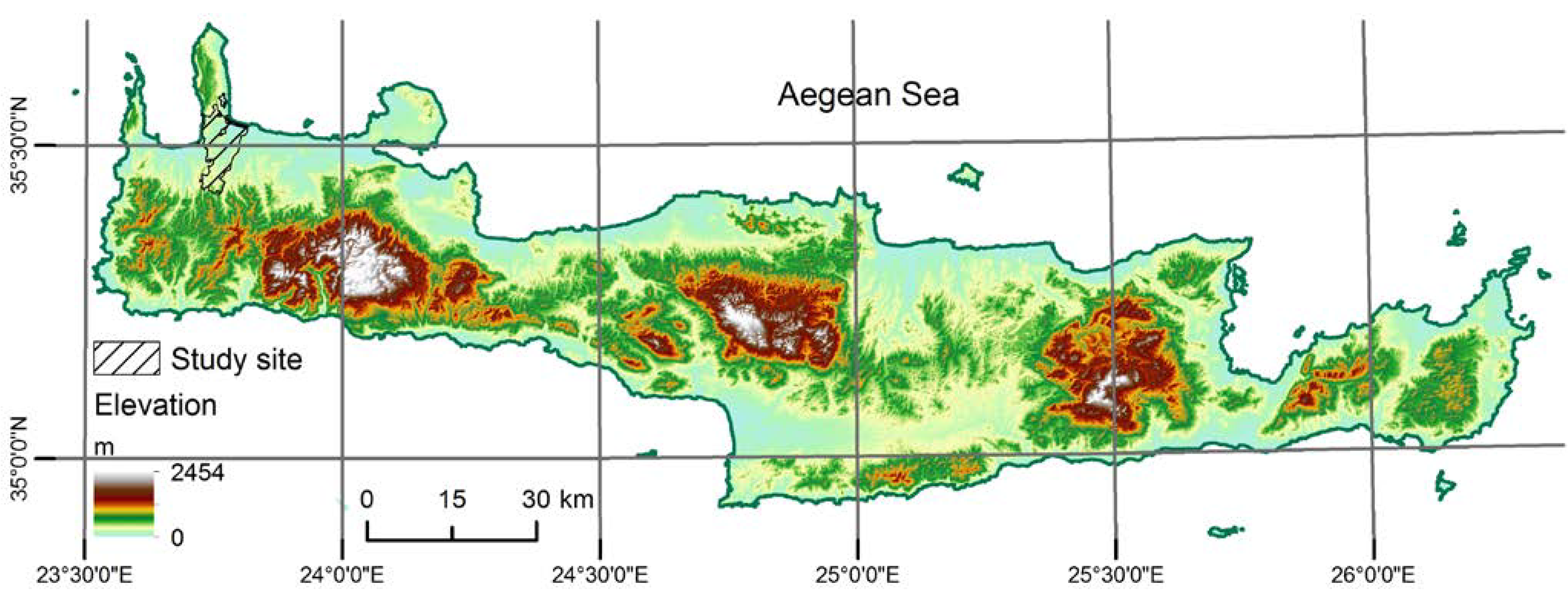
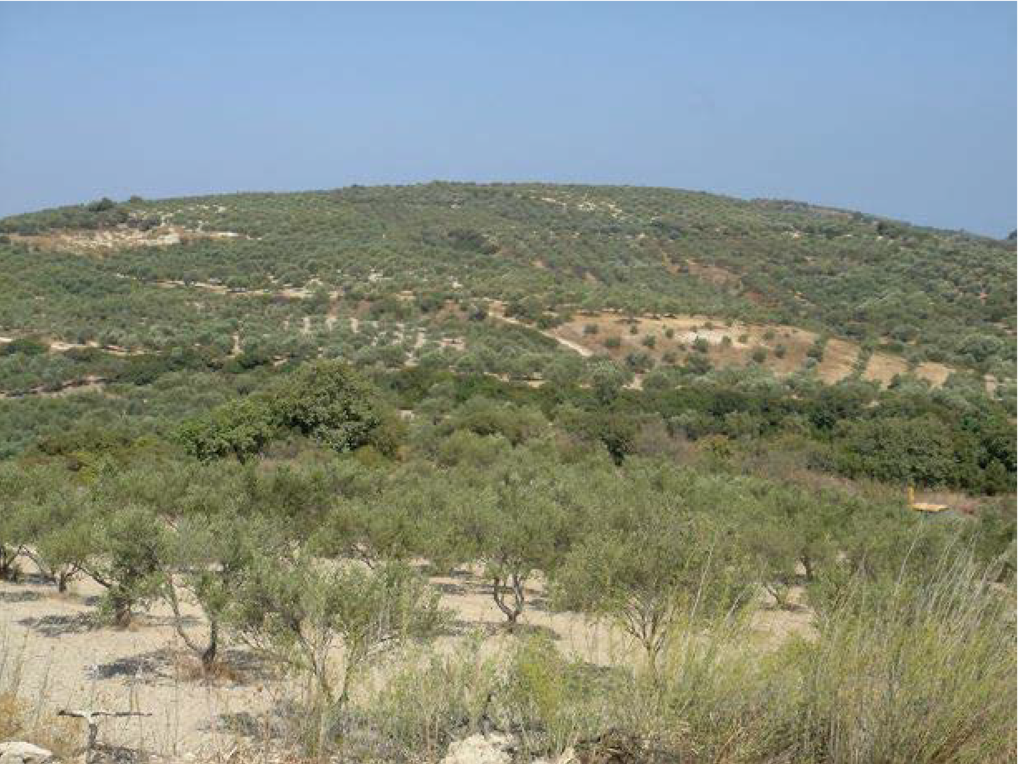
2.1. Study Area

The agricultural area of the Municipality of Kolymvari was selected as the study site. Kolymvari contains 17 villages and is located in the NW part of Crete, Greece, about 20 km west of the city of Chania (latitude/longitude: 35°30'00"/23°46'00") (Figure 1). The main activity in the area is agriculture, mainly olive plantations. The agricultural area of interest was outlined based on information derived from the CORINE 2000 land cover/use map and was further refined with visual photo-interpretation of a QuickBird (very high resolution) satellite image. The total extent of the agricultural study site was about 69 km².

Figure 1. The agricultural area of Kolymvari, Crete.

Figure 1. The agricultural area of Kolymvari, Crete.

The climate of the area is typically Mediterranean, with hot and very dry summers. Winters are mild, seldom experiencing frosts. The mean annual air temperature is 17 °C. Most of the rainfall takes place during winter, especially in the mountains. The average annual rainfall is 722.6 mm, with January (143.8 mm) and July (0.6 mm) being the wettest and the driest months, respectively. From late April to early September, rainfall is unusual, but it may occur in every month, even in July.

The terrain of the area is undulating, with an alteration of mountainous, semi-mountainous and plain landscapes throughout the area, which is vulnerable to erosion in terms of main topsoil characteristics. According to the EU soil map on a scale of 1:1,000,000, two soil types are predominant in the area of Kolymvari:

Rendzina soils, i.e., soils with A and C horizons, a well-developed A1 horizon of heavy texture, including gravels, about 50 cm high, with over 30% free calcium carbonate and Terra rosa soils, i.e., heavy soils with A, B, and C horizons, having a reddish textural B horizon and with poor drainage and poor permeability. A soil horizon is a layer parallel to the soil surface, whose physical characteristics differ from the layers above and beneath. More specifically, A-horizon is a surface layer of mineral soil with most organic matter accumulation and soil life; B-horizon is a subsoil layer accumulating iron, clay, aluminum and organic compounds, a process referred to as illuviation; and C-horizon is a parent rock layer (with large unbroken rocks) usually accumulating the more soluble compounds [18].

The primary sector is predominant in Kolymvari (55%), with the main agricultural activity occupied by olive tree cultivation for olive oil production. The area produces approximately 65,000 tons of olive oil per year, treated by 17 olive-oil factories. Similarly with many other Mediterranean regions, large areas in Kolymvari have been altered during the last 25 years by replanting high-density olive plantations in semi-mountainous and coastal areas. As a consequence, intensive tillage and soil compaction from farm machinery on shallow soils in the uplands have rendered big areas especially vulnerable to soil erosion [19] (Figure 2).

Figure 2. Olive plantations in Kolymvari.

Figure 2. Olive plantations in Kolymvari.

2.2. Dataset Description

The dataset collected and processed for the study comprised the following records:

• Geological map sheets of the area on a 1:50,000 scale. The map sheets were scanned and merged into a mosaic in order to derive a single geologic background. Then, the outlines of the geologic units were digitized;
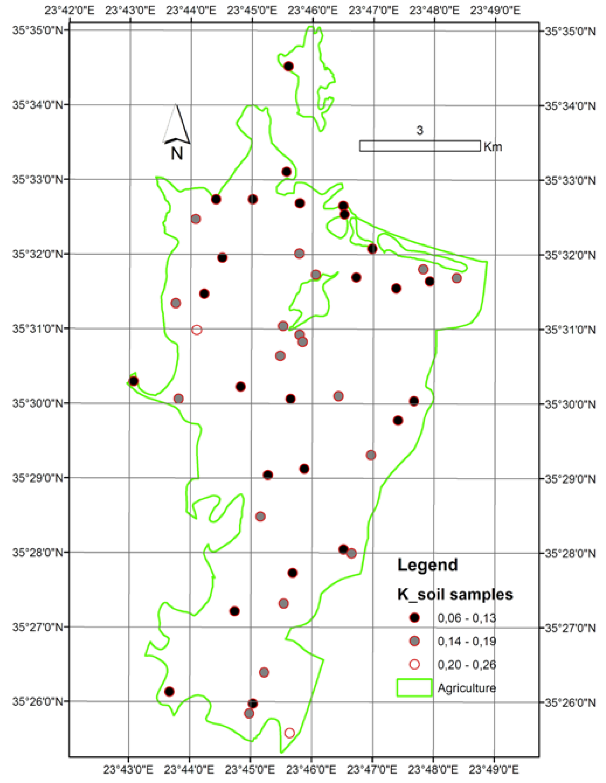
• Soil data retrieved with a field survey at 45 sampled locations randomly selected throughout the study area after stratification according to the geologic units. The density of sampling was estimated in one sample per 1.5 km² on average. It was estimated that sampled points were allocated into homogeneous sub-areas and, thus, were representative of their sites.
• The samples were extracted from the topsoil (depth <15 cm). Fine silt and sand percentage, organic matter content, permeability class and structure class were calculated in the laboratory after international soil analysis standards;
• A yearly distribution of the mean monthly rainfall in the study area calculated from 22-year long recordings (1971–1992) and derived from two meteorological stations in the area, namely Drapanias and Tavronitis stations;
• A digital elevation model (DEM) of the study area, created from available point raster files with 20 m resolution as (x,y,z) files, with non-linear rubber sheeting and an output cell size of 4 m. The RMS error in z (elevation) was found to be 5.21 m after testing at 33 trigonometric points; and
• A QuickBird satellite image acquired on November 16, 2002, covering a swath of 16.5 km by 16.5 km, with a good geometric accuracy. The image was the result of orthorectification and fusion of the panchromatic (gray scale) and multispectral components in the laboratory. The final product was a 0.62 m pixel size image with four spectral bands.

All geographical data were projected into the Greek grid coordinate system (datum: GGRS87).

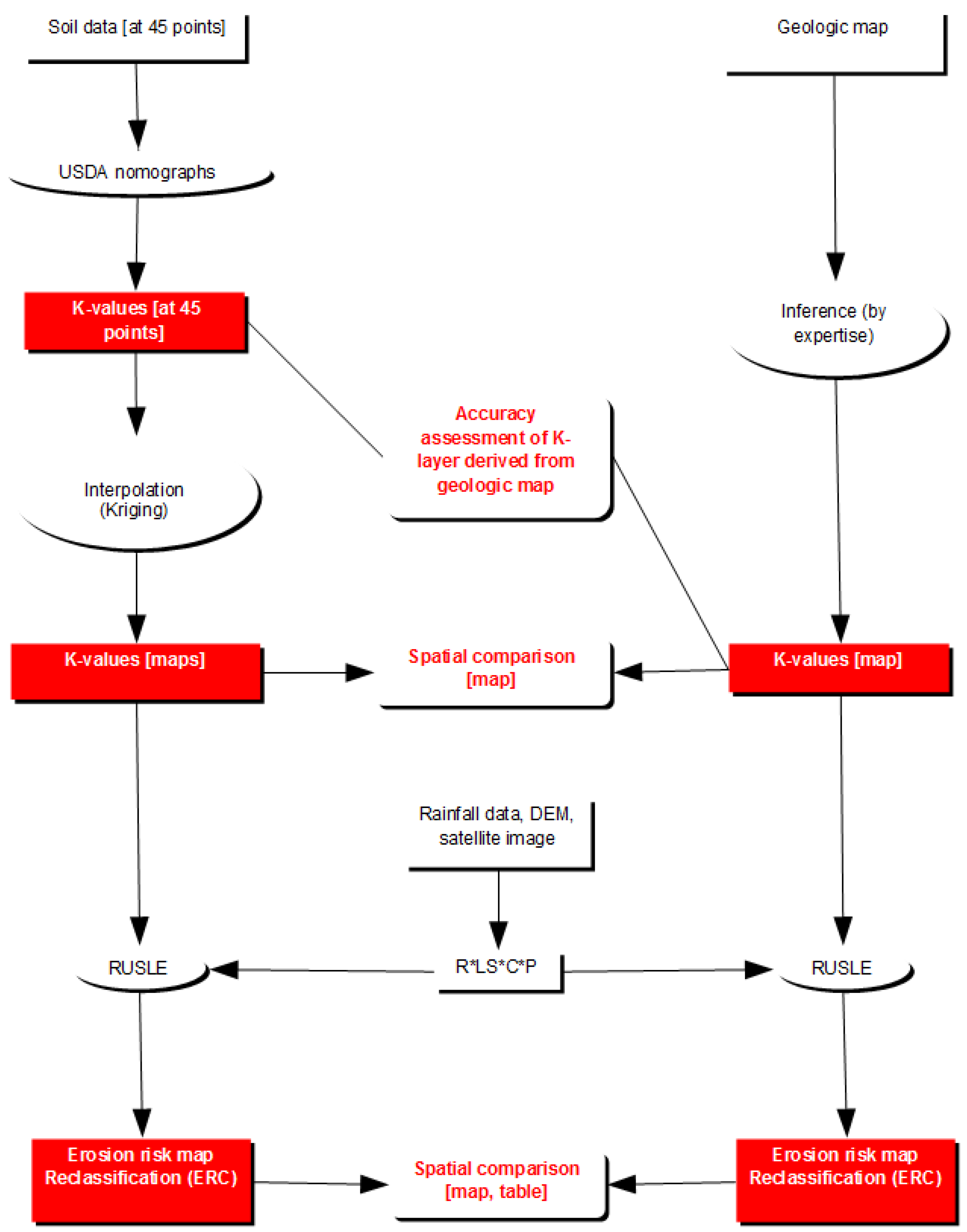
2.3. Methodology Overview

The methodology was based on the principles and formulas of RUSLE (revised universal soil loss equation) and was implemented in the spatial domain using raster GIS. RUSLE was evolved from USLE (universal soil loss equation) with incorporation of more validation data [20]. Although RUSLE was originally developed for application at the parcel scale, a topographic extension proposed by [21] rendered the model appropriate for predicting annual soil erosion rates of small catchments. The mathematical expression of RUSLE is [3]:

A = R × K × LS × C × P

(1)

where A is the average annual erosion rate (t ha⁻¹), R is the rainfall erosivity (MJ cm ha⁻¹ h⁻¹), K is the soil erodibility (t ha h MJ⁻¹ ha⁻¹ cm⁻¹), L is the slope length (dimensionless), S is the slope steepness (dimensionless), C is the vegetation cover and management factor (dimensionless) and P is the support practice factor (dimensionless).

In this study, the K-factor (soil erodibility) was estimated firstly from the geologic map with inference (use of expertise) by an independent soil scientist. Secondly, K-values were calculated at the 45 sampled locations using the K-nomographs (known also as USDA nomographs) [3]. Then, the latter set of K-values was used as reference in order to assess the accuracy of K-values derived from the geologic map.

Later, a new K-layer was generated with Ordinary Kriging interpolation of the K-values calculated at the sampled locations, using a spherical semivariogram and 12 points in the neighborhood. The K-layers derived from both alternatives were spatially compared. In parallel, all the rest of the erosion factors (i.e., R, LS, C and P) were generated also as GIS layers according to the RUSLE literature and the available dataset. Finally, the mapping results of soil erosion risk derived from both alternatives were spatially compared. A workflow of the methodology is shown in Figure 3, while all the steps are discussed in detail in the following paragraphs.

Figure 3. Workflow of the methodology.

Figure 3. Workflow of the methodology.

2.4. K-Values Derived from the Geological Map

Estimation of K-values from the geological map by inference is analyzed in the following two steps (Table 1):

• Determination of the soil texture class for each type of geological formation found in the study site based on soil genesis rules [22]. Soil texture is a parameter strongly influenced by the process of soil formation, due to rock weathering. It must be noted, though, that different geologic formations may result in the same or different soil textures.
• Conversion of the soil texture value into a K-value according to the knowledge of the local conditions, especially regarding physiographic processes and levels of organic matter content in the area. The physiography of Kolymvari is characterized as hilly to semi-mountainous, while the organic matter levels range between 0% and 6% (3% on average).

Table 1. K-values inferred from the geological formations with expertise.

Parent material (geologic map)	Soil texture *	K-value
Alluvial deposits	SL–L	0.15
Limestone	C, SiC	0.4
Peridotite	CL–C	0.5
Granite	S–SL	0.2
Schists	L	0.7
Gneiss	S, LS,L	0.3
Tertiary deposits	SL–L	0.15

* C = clay, CL= clay loam, L = loam, LS = loamy sand, S = sand, SC = sandy clay, SL = sandy loam, Si = silt, SiC= silty clay, SiCL = silty clay loam, SIL = silt loam.

Table 1. K-values inferred from the geological formations with expertise.

Parent material (geologic map)	Soil texture *	K-value
Alluvial deposits	SL–L	0.15
Limestone	C, SiC	0.4
Peridotite	CL–C	0.5
Granite	S–SL	0.2
Schists	L	0.7
Gneiss	S, LS,L	0.3
Tertiary deposits	SL–L	0.15

* C = clay, CL= clay loam, L = loam, LS = loamy sand, S = sand, SC = sandy clay, SL = sandy loam, Si = silt, SiC= silty clay, SiCL = silty clay loam, SIL = silt loam.

2.5. K-Values Derived from the Soil Samples

Estimation of K-values from soil data (45 samples) was based on the formulas developed by [3], which are available also in the form of nomographs (USDA nomographs). The samples were tested for spatial autocorrelation of all numerical soil parameters (organic matter, fine silt and sand): Morans I test indicated random samples for all parameters, only somewhat clustered due to the stratification. Laboratory analysis of the samples included sand content, silt and fine sand content (in percentages), organic matter content (in percentage) and qualitative classifications of soil structure (four classes) and permeability (seven classes). Calculation of soil texture was achieved with the Bouyoucos method, while for the organic matter content, the Walkley-Black method was employed. Soil structure and permeability was evaluated in the field by the soil experts who conducted the survey. The sampled locations and the K-values calculated with K-nomographs are shown in Figure 4.

2.6. Generation of K-Layers

Two alternative methodologies were implemented for creating K-layers from the available data (i.e., the geological map and the sampled soil properties):

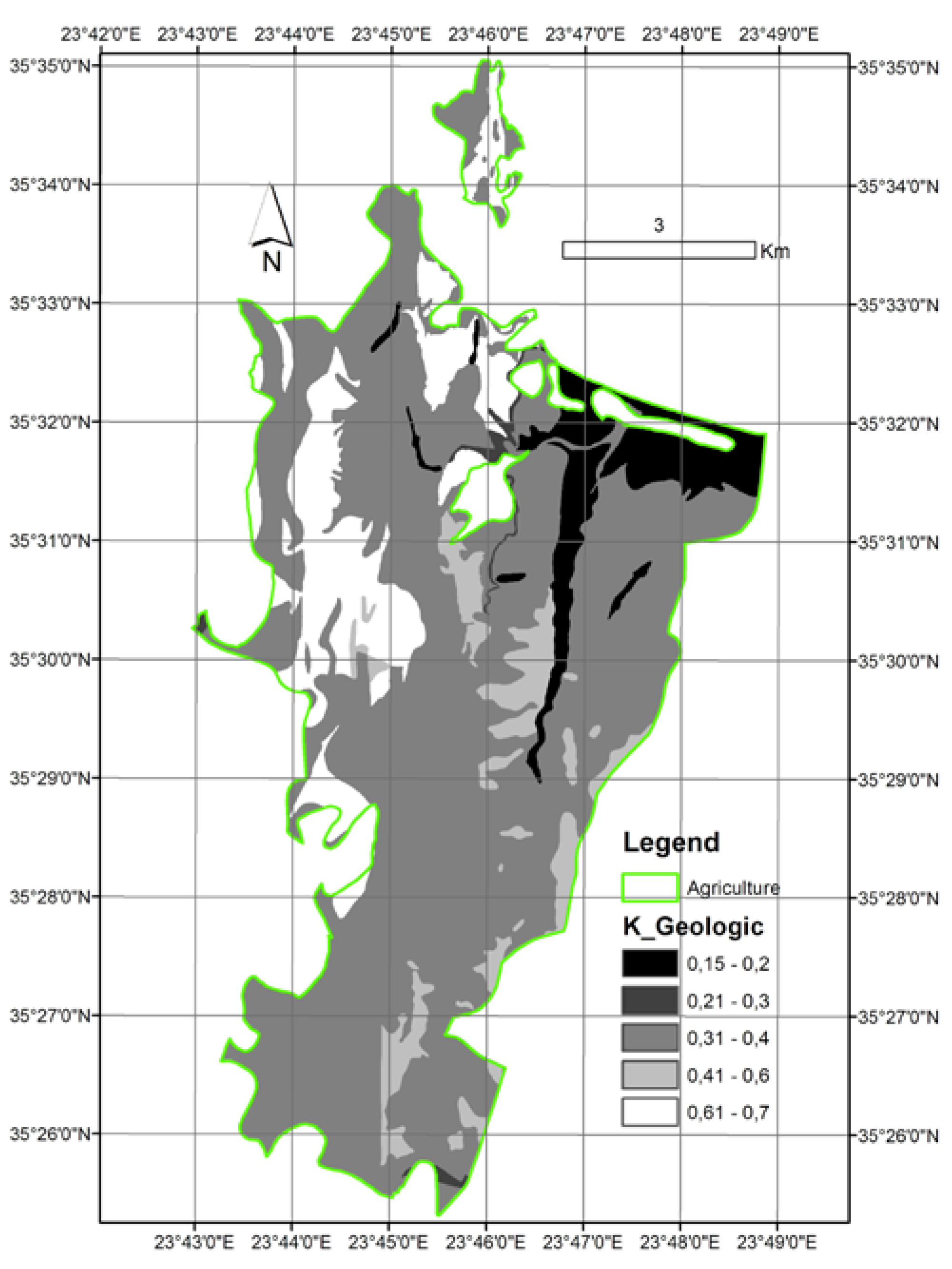
• A layer where a single K-value was assigned to each geologic formation according to the interpretation made (based on soil genesis rules) by the soil expert (Figure 5); and
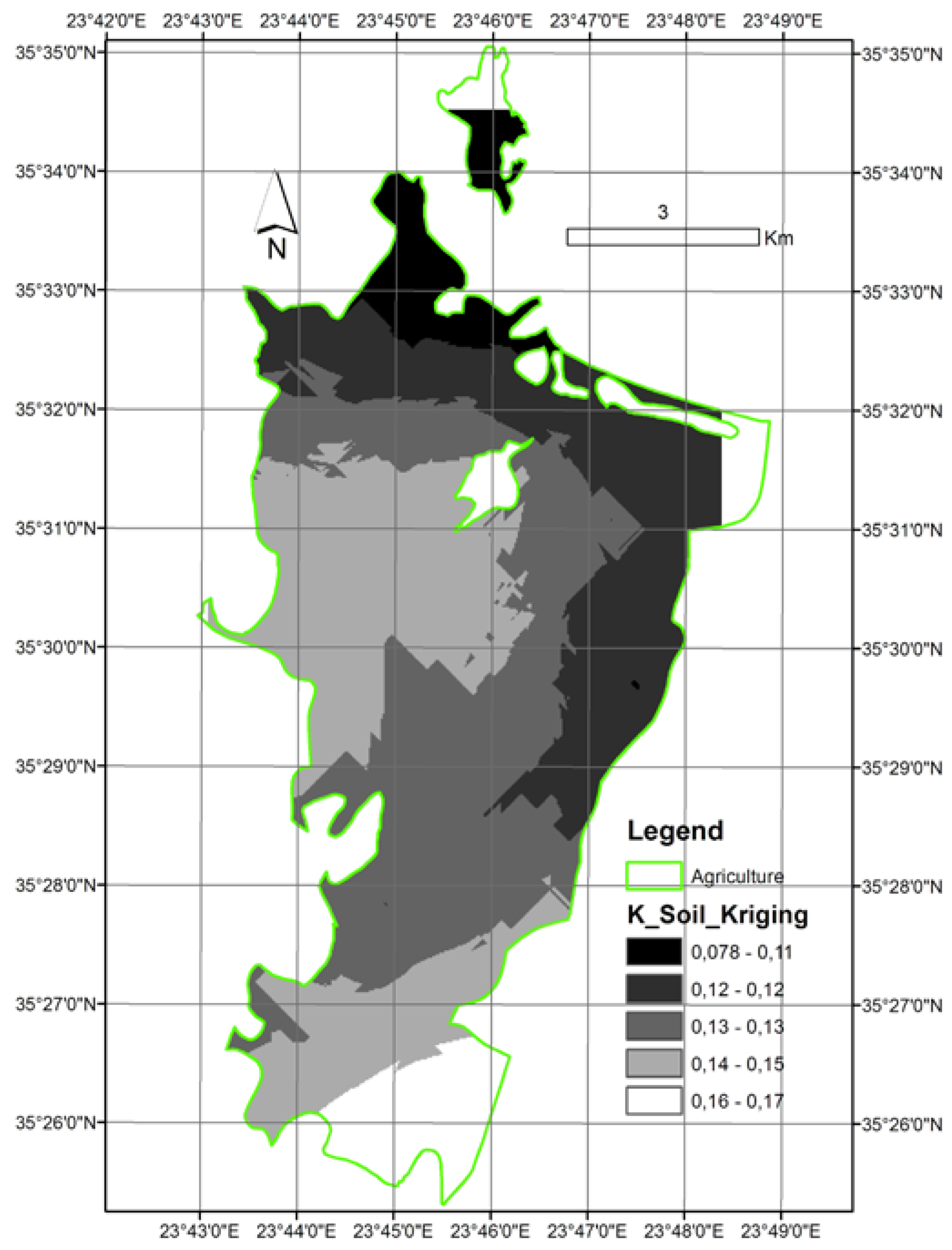
• A layer generated with spatial interpolation of the K-values calculated with the K-nomographs at the sampled locations. Interpolation is the procedure of predicting the value of attributes at un-sampled sites from measurements made at point locations within the same area. There are several interpolation methods with contradicting references about their performance. In this study, Ordinary Kriging interpolation was employed, as it is reported to perform better for non-grid sampling schemes [23,24] (Figure 6).

Figure 4. The sampled locations and the calculated soil erodibility (K) values.

Figure 4. The sampled locations and the calculated soil erodibility (K) values.

Figure 5. K-layer derived from the geologic map by expertise.

Figure 5. K-layer derived from the geologic map by expertise.

Figure 6. K-layer derived with Ordinary Kriging of K-values calculated at the soil-sampled locations with USDA nomographs.

Figure 6. K-layer derived with Ordinary Kriging of K-values calculated at the soil-sampled locations with USDA nomographs.

2.7. Generation of R, LS, C and P Layers

Given that a detailed description of the implemented methods for generation of the R, LS, C and P layers is out of the scope of this paper, only a short summary of these methodologies is provided below:

• The R-factor (climate attributes) was estimated using a regression of precipitation versus elevation, as it is accepted that climate varies strongly with elevation. Elevation is an excellent statistical predictor variable, because it is sampled at a far greater spatial density than climate variables and is often estimated on a regular grid (i.e., DEM). Extrapolation of the two stations’ data in this study was done by linear regression [25];
• The LS-factor (terrain attributes) was derived based on the D8 (deterministic-eight node) algorithm, which takes into account the 3 × 3 matrix moving on a DEM starting from the inner grid cell and analyzes the relationship with the neighboring cells [26];
• The C-factor (vegetation attributes) was derived from the NDVI (normalized difference vegetation index) after conversion with a monotonically decreasing sigmoid function with two control inflection points (zero and one). NDVI expresses the coverage potential of vegetation, and because the area is covered by permanent crops, the season of image acquisition (November) was appropriate for differentiating the presence and conditions of green vegetation in the study site [27,28]; and
• The P-factor (management attributes) was estimated by allocating features protective to soil erosion, e.g., terraces and roads parallel to the contours, with image processing techniques applied on the QuickBird imagery [29].

3. Results and Analyses

3.1. Accuracy Assessment of K-values Derived from the Geologic Map

K-values extracted from the soil samples were used as reference in order to assess the accuracy of K-values derived from the geological map. Cross-analysis of the two independent datasets of K-values resulted in a 0.1475 RMS error. It should be noted though that soil structure and permeability were not measured in the field or lab, but rather, were estimated by expertise.

The datasets went also under matched pair analysis, which is appropriate when two responses from a pair of measurements coming from the same experimental unit are to be compared [30]. The comparison resulted in a mean difference value of −0.2991, a standard error value of 0.02353, a correlation value of −0.0757 and a t-Ratio value of −12.7136 (Figure 7). These results show that K-values estimated from the geological map were completely unreliable if K-values derived from the soil data are to be taken as ground truth. It is obvious that the assumption about undisturbed soils, implied when extracting K-values from geological data, was not met in a very great degree.

Figure 7. Top: distributions of K-values derived from the geologic map; middle: distributions of K-values derived from the soil samples; bottom: matched pairs analysis of the K-datasets.

Figure 7. Top: distributions of K-values derived from the geologic map; middle: distributions of K-values derived from the soil samples; bottom: matched pairs analysis of the K-datasets.

3.2. Comparison of K-Layers

Because matched pairs analysis showed a big mean difference and almost no correlation between the two sets of K-values, the K-layers were compared using a normalized difference. Normalized difference values lie in a range of [−1,+1], thus making standardized map comparisons possible.

The results of the spatial numerical comparison of the two maps showed the following:

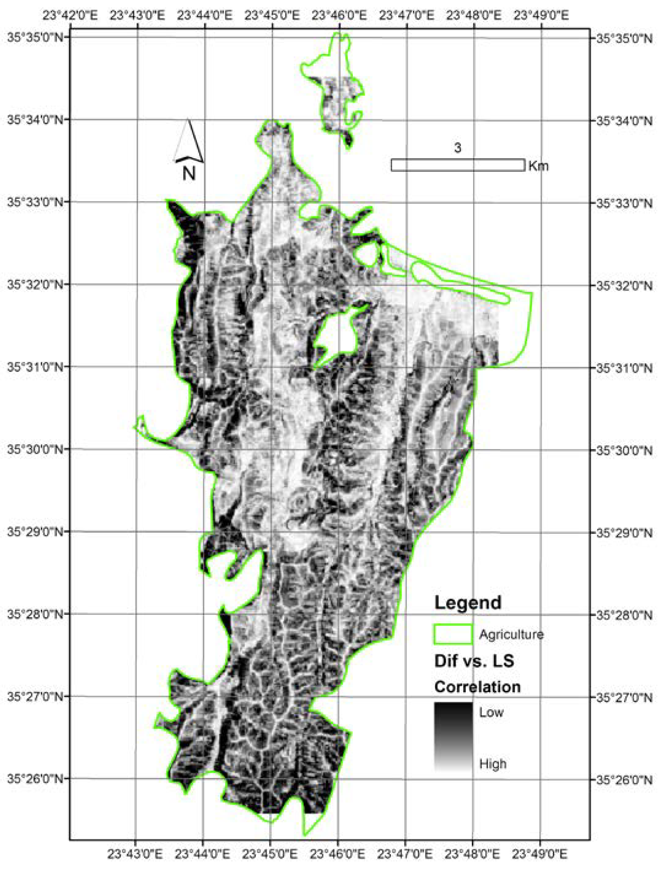
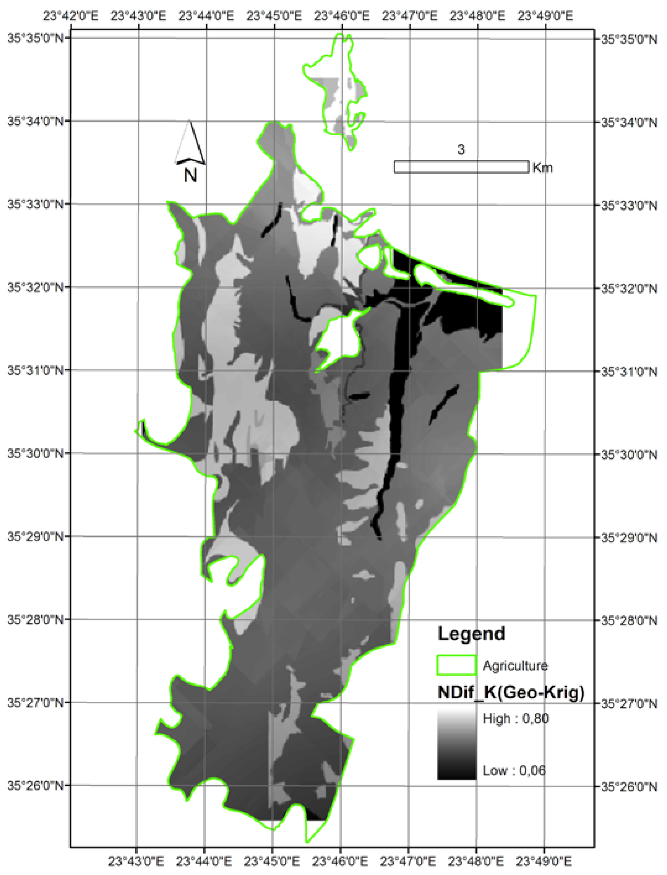
• The pattern of the geological map was predominant in the difference map. This was expected, given the fact that values change distinctly in the geologic map, whereas values change gradually in interpolation surfaces (Figure 8).
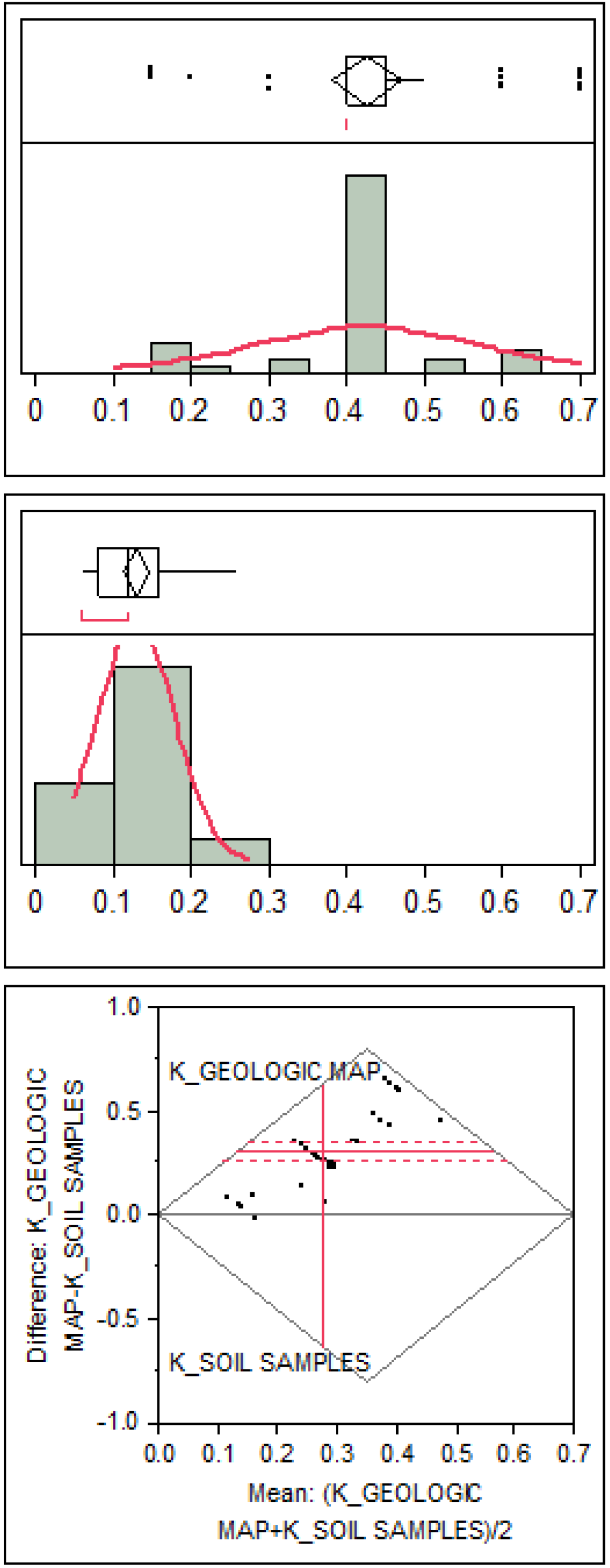
• A big mean normalized difference (0.52) was found between the two K-layers, while for the great extent of the study area, the normalized difference was larger than 0.40.

Figure 8. Normalized difference map of K-values derived from the two alternatives.

Figure 8. Normalized difference map of K-values derived from the two alternatives.

Moreover, the difference map (NDif = K(geo) − K(soil)) was tested for its spatial correlation (SC) to the other erosion factor (EF) layers. This was achieved with a simple technique, i.e., by multiplying the erosion factor layers with a complementary difference map (Formula 2). Low values resulting from this operation indicate cells where the correlation between the specific erosion factor and the difference map was high.

SC(EF) = EF × (1 − NDif)

(2)

The tests showed a high correlation of LS-factor (topographic attributes) with the difference map in some specific areas (Figure 9), while a medium correlation of C-factor (vegetation attributes) with the difference map was observed for the entire area. Under certain conditions, these observations could lead to a justification of the reasoning for the differences in K estimations.

Figure 9. Spatial correlation of the terrain attributes (LS-layer) with the difference (NDif) map.

Figure 9. Spatial correlation of the terrain attributes (LS-layer) with the difference (NDif) map.

3.3. Comparison of Erosion Risk Maps

The availability of two alternative K-layers led to the generation of two erosion risk maps using map algebra according to the RUSLE literature and formulas:

• One using as input the K-layer derived from the geologic map; and
• One using as input the K-layer derived from the soil samples with Ordinary Kriging interpolation.

The resulting soil erosion risk maps were then reclassified into five erosion risk classes (ERC), according to [3] (Table 2) and compared (Figure 10).

Table 2. Erosion risk classes (ERC) proposed by Wischmeier and Smith (1978).

Erosion class	ERC1	ERC2	ERC3	ERC4	ERC5
Loss t/ha/year	0–5	5–10	10–20	20–40	>40
Classification	Very slight	Slight	Moderate	Severe	Very severe

Table 2. Erosion risk classes (ERC) proposed by Wischmeier and Smith (1978).

Erosion class	ERC1	ERC2	ERC3	ERC4	ERC5
Loss t/ha/year	0–5	5–10	10–20	20–40	>40
Classification	Very slight	Slight	Moderate	Severe	Very severe

Figure 10. Map of identical risk classification (ERC = 5) by both alternatives.

Figure 10. Map of identical risk classification (ERC = 5) by both alternatives.

Examination of the ERC map derived from the geologic map showed that only 7.3% of the area was classified in the three low classes of severity, while the greatest part of the area (92.7%) was classified within the highest severity classes (ERC4 and ERC5). On the other hand, in the ERC map based on soil sampling, the low severity classes covered 17.6% of the area, while the rest (82.4%) belonged to the two highest severity classes (Table 3). These figures show that the alternatives resulted in similar patterns, although there is significant difference between them with regard to the coverage of ERC5 (87.3% vs. 66.8%). Original erosion rates based on the geologic map were estimated to be about 20% higher than those based on soil sampling. However, the original difference between the K-layers was significantly reduced in the ERC maps.

Table 3. Extent of ERCs in the study area.

Methods	K from geologic map		K from interpolated K values
Erosion Risk Class	Extent (ha)	Proportion of ERC over the total study area (%)	Extent (ha)	Proportion of ERC over the total study area (%)
Very slight—ERC1	105	1.5	225	3.4
Slight—ERC2	162	2.3	344	5.2
Moderate—ERC3	244	3.5	601	9.0
Severe—ERC4	373	5.4	1037	15.6
Very severe—ERC5	6039	87.3	4474	66.8
Total	6923	100	6681 *	100

* The difference in total acreage is due to the fact that the areas beyond peripheral sampling points were excluded from the interpolation.

Table 3. Extent of ERCs in the study area.

Methods	K from geologic map		K from interpolated K values
Erosion Risk Class	Extent (ha)	Proportion of ERC over the total study area (%)	Extent (ha)	Proportion of ERC over the total study area (%)
Very slight—ERC1	105	1.5	225	3.4
Slight—ERC2	162	2.3	344	5.2
Moderate—ERC3	244	3.5	601	9.0
Severe—ERC4	373	5.4	1037	15.6
Very severe—ERC5	6039	87.3	4474	66.8
Total	6923	100	6681 *	100

* The difference in total acreage is due to the fact that the areas beyond peripheral sampling points were excluded from the interpolation.

Additional to the non-spatial statistical comparison (Table 3), the alternative methods were compared spatially using the cross-tabulation method. Cross-tabulation displays the joint distribution of a variable derived from two different sources in a table. In this case, the classes derived from soil sampling are set vertically, and the classes derived from the geologic map are set horizontally. The numbers of cells that resulted in the same class for both methods are found diagonally (Table 4).

Table 4. Cross-tabulation matrix of ERC derived from the alternatives (number of cells).

Soil samples	Geologic map					Totals
	ERC-1	ERC-2	ERC-3	ERC-4	ERC-5
ERC-1	1,083	904	796	247	104	3,134
ERC-2	119	886	1,218	1,889	699	4,811
ERC-3	30	139	935	1,949	5,346	8,399
ERC-4	5	24	131	718	13,612	14,490
ERC-5	0	3	40	178	62,174	62,395
Totals	1,237	1,956	3,120	4,981	81,935	93,229

Table 4. Cross-tabulation matrix of ERC derived from the alternatives (number of cells).

Soil samples	Geologic map					Totals
	ERC-1	ERC-2	ERC-3	ERC-4	ERC-5
ERC-1	1,083	904	796	247	104	3,134
ERC-2	119	886	1,218	1,889	699	4,811
ERC-3	30	139	935	1,949	5,346	8,399
ERC-4	5	24	131	718	13,612	14,490
ERC-5	0	3	40	178	62,174	62,395
Totals	1,237	1,956	3,120	4,981	81,935	93,229

From Table 4, it can be derived that the maps differ significantly in ERC2, ERC3 and ERC4, while they are similar in ERC1 and ERC5. In an overall comparison of the two maps, they demonstrate a moderate to high level of similarity, since they match, in terms of ERC, 70.5%. This means that more than 70% of the area was classified in the same severity class by both alternatives. Especially for ERC5, the level of similarity exceeds 76%. If ERC4 and ERC5 are grouped together, the level of similarity between the two method alternatives exceeds 88%.

4. Conclusions

The K-layer generated from the geologic map by inference was significantly unreliable (RMS error of 0.1475), showing that—at least in the case of Kolymvari—human expertise was of limited value in the erosion risk mapping procedure with RUSLE. Low reliability could be attributed to the following reasons:

• The study area was highly disturbed by anthropogenic activities (long agricultural history), rendering the assumptions made about undisturbed soils non-realistic;
• The soil expert considered that the area was very poor in organic matter, which was proved not to be true. Based on average Greek standards, an assumption was made for values <2%, while the mean value was found to be 3%. As a consequence, the inferred K-values were overestimated; and
• Unlike a physiographic map, a geologic map contains limited information, rendering estimations by inference much more uncertain.

Statistical comparison of K-values estimated from the alternative datasets at the same points resulted in significant differences, i.e., a mean difference value of −0.2991, a standard error value of 0.02353 and a correlation value of −0.0757. This shows that K-datasets were not correlated, and therefore, the error was not systematic. This fact could be attributed to the following reasons:

• Some specific soil properties might have affected soil erodibility more than others and, moreover, by a different degree throughout the study site. This idea has been expressed originally by [16]; and
• Some of the sampled soil properties were not measured, but estimated by expertise (good knowledge of the study site from previous work). These properties were the soil structure and permeability, which are reported to be of high importance in estimating K. This fact increased uncertainty in K-estimations from soil properties.

A correlation test of the difference K-map to the other erosion factor layers, i.e., R, LS, C and P, showed:

• High correlation with the LS-layer in some specific areas, which means that in these areas, the topography was a major attributor to the different estimations by the two alternatives. This observation is in line with the suggestion of using physiographic maps instead of soil maps made by [16]; and
• Medium correlation with the C-layer for the entire area, which means that the vegetation cover was a standard moderate attributor to the error.

Under certain conditions, the above observations can lead to more specific justifications of the differences in K-estimations by the alternative methods.

As it was expected, the differences in K-estimations were transferred to the erosion maps through the use of RUSLE formula. However, when erosion risk values were ranked into five classes of severity (ERC), the dissimilarities observed in the K-layers faded out. More specifically:

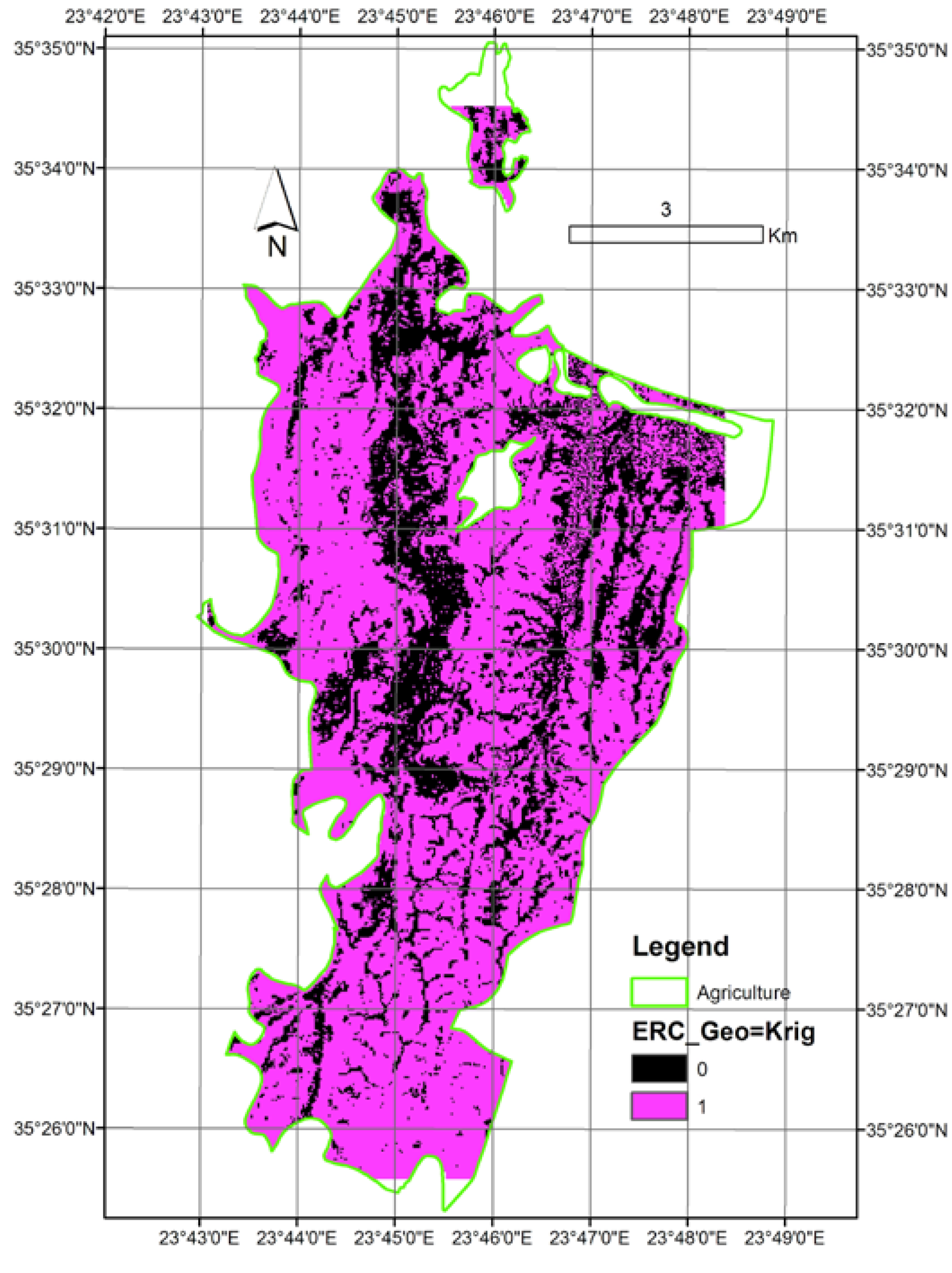
• The reclassification in ERC resulted in an overall similarity of the two erosion maps, which exceeded 70%;
• Moreover, in ERC5, the level of similarity exceeded 76%; and
• Regrouping ERC4 and ERC5 resulted in a level of similarity between the two alternatives, which exceeded 88%.

In summary, it was confirmed that soil-related data quality is a crucial parameter in K-factor estimation. Furthermore, errors in data collection and interpretation were clearly propagated to the erosion maps. Reclassification of the erosion rates, however, eliminated the impact of initial uncertainties, as the hot spots allocated by ERC4 and ERC5 were identical for 88% of the study site for both alternatives. This fact confirmed the basic hypothesis of the study and emphasized RUSLE as a decision support tool.

A question arising from this research is whether and how much a fine-scale geologic map could improve the accuracy of K-values when the expertise alternative is followed. On the other hand, if a denser grid of sampling sites for the soil survey approach would produce a better K-layer after interpolation, such a procedure would be costly and time-consuming.

Future research will focus on mapping K-factors with object-based analysis, thus giving importance to:

• Different sources of soil information (geologic, physiographic, soil and imagery datasets); and
• Soil-related patterns as an additional parameter of soil erodibility.

Obviously, there is a need for bigger and complete reference datasets and for additional study sites towards model calibration and testing. Also, new methods, including fuzzy sets, could be used in describing K-values and their distribution and categorization, as suggested by [31].

References

1. Foster, G.R.; Meyer, L.D. A Closed-form Soil Erosion Equation for Upland Areas. In Sedimentation Symposium in Honor Porf. H.A. Einstein; Sten, H.W., Ed.; Colorado State University: Ft. Collins, CO, USA, 1972; pp. 12:1–12:19. [Google Scholar]
2. Sanders, D.W. Sloping Land: Soil Erosion Problems and Soil Conservation Requirements. In Land Evaluation for Land-use Planning and Conservation in Sloping Areas; Siderius, W., Ed.; Institute for Land Reclamation and Improvement: Wageningen, The Netherlands, 1986; pp. 40–50. [Google Scholar]
3. Wischmeier, W.H.; Smith, D.D. Predicting Rainfall Erosion Losses from Cropland East of the Rocky Mountains; Agricultural Research Service, U. S. Department of Agriculture in Cooperation with Purdue Agricultural Experiment Station: Washington, DC, USA, 1978. [Google Scholar]
4. Kinnell, P.I.A. Raindrop-impact-induced erosion processes and prediction: A review. Hydrol. Process. 2005, 19, 2815–2844. [Google Scholar] [CrossRef]
5. Le Bissonnais, Y.; Cerdan, O.; Lecomte, V.; Benkhadra, H.; Souchere, V.; Martin, P. Variability of soil surface characteristics influencing runoff and interril erosion. Catena 2005, 62, 111–124. [Google Scholar] [CrossRef]
6. Aksoy, H.; Kavvas, M.L. A review of hillslope and watershed scale erosion and sediment transport models. Catena 2005, 64, 247–271. [Google Scholar] [CrossRef]
7. De Vente, J.; Poesen, J. Predicting soil erosion and sediment yield at the basin scale: Scale issues and semi-quantitative models. Earth Sci. Rev. 2005, 71, 95–125. [Google Scholar] [CrossRef]
8. Garcia-Ruiz, J.M. The effect of land uses on soil erosion in Spain: A review. Catena 2010. [Google Scholar] [CrossRef]
9. Boardman, J. Soil erosion science: Reflections on the limitations of current approaches. Catena 2006, 68, 73–86. [Google Scholar] [CrossRef]
10. Proposal for a Directive of the European Parliament and of the Council Establishing a Framework for the Protection of Soil and Amending Directive 2004/35/EC; European Commission: Brussels, Belgium, 2006.
11. Integration of Environment into EU Agriculture Policy; The IRENA Indicator-Based Assessment Report; København, K. (Ed.) European Environment Agency: Copenhagen, Denmark, 2006.
12. Millington, A.C. Reconnaissance Scale Soil Erosion Mapping Using a Simple Geographic Information System in the Humid Tropics. In Land Evaluation for Land-use Planning and Conservation in Sloping Areas; Siderius, W., Ed.; Institute for Land Reclamation and Improvement: Wageningen, The Netherlands, 1986; pp. 64–81. [Google Scholar]
13. Merritt, W.S.; Letcher, R.A.; Jakeman, A.J. A review of erosion and sediment transport models. Environ. Model. Softw. 2003, 18, 761–799. [Google Scholar] [CrossRef]
14. Karydas, C.G.; Panagos, P.; Gitas, I.Z. A classification of water erosion models according to their geospatial characteristics. Int. J. Dig. Earth 2002, 16, 663–680. [Google Scholar] [CrossRef]
15. Van Rompaey, A.J.J.; Govers, G. Data quality and model complexity for regional scale soil erosion prediction. Int. J. Geogr. Inf. Sci. 2002, 16, 663–680. [Google Scholar]
16. Perez-Rodriguez, R.; Marques, M.J.; Bienes, R. Spatial variability of the soil erodibility parameters and their relation with the soil map at subgroup level. Sci. Total Environ. 2007, 378, 166–173. [Google Scholar]
17. Jetten, V.; de Roo, A.; Favis-Mortlock, D. Evaluation of field-scale and catchment-scale soil erosion models. Catena 1999, 37, 521–541. [Google Scholar]
18. IUSS Working Group WRB, World Reference Base for Soil Resources 2006, 2nd ed.; World Soil Resources Reports No. 103; FAO: Italy, 2006.
19. Beaufoy, G. The Environmental Impact of Olive Oil Production in European Union (Report); European Forum on Nature Conservation and Pastoralism: Madrid, Spain, 2000. [Google Scholar]
20. Renard, K.; Foster, G.R.; Weesies, G.A.; Porter, J.P. RUSLE Revised universal soil loss equation. J. Soil Water Conserv. 1991, 46, 30–33. [Google Scholar]
21. Desmet, P.; Grovers, G. A GIS procedure for automatically calculating the USLE LS factor on topographically complex landscape units. J. Soil Water Conserv. 1996, 51, 427–433. [Google Scholar]
22. Buol, S.W.; Southard, R.J.; Graham, R.C.; McDaniel, P.A. Soil Genesis and Classification, 5th ed.; Iowa State University Press: Ames, IA, USA, 2003; p. 494. [Google Scholar]
23. Mueller, T.G.; Pusuluri, N.B.; Mathias, K.K.; Cornelius, P.L.; Barnhisel, R.I.; Shearer, S.A. Map quality for ordinary kriging and inverse distance weighted interpolation. Soil Sci. Soc. Am. 2001, 68, 2042–2047. [Google Scholar]
24. Schloeder, C.A.; Zimmerman, N.E.; Jacobs, M.J. Comparison of methods for interpolating soil properties using limited data. Soil Sci. Soc. Am. 2001, 65, 470–479. [Google Scholar] [CrossRef]
25. Daly, C.; Gibson, W.P.; Taylor, G.H.; Johnson, G.L.; Pasteris, P. A knowledge-based approach to the statistical mapping of climate. Climate Res. 2002, 22, 99–113. [Google Scholar] [CrossRef]
26. Gallant, J.C.; Wilson, J. TAPES-G: A grid-based terrain analysis program for the environmental sciences. Comput. Geosci. 1996, 22, 713–722. [Google Scholar] [CrossRef]
27. De Jong, S.M.; Paracchini, M.L.; Bertolo, F.; Folving, S.; Megier, J.; de Roo, A.P.J. Regional assessment of soil erosion using the distributed model SEMMED and remotely sensed data. Catena 1999, 37, 291–308. [Google Scholar] [CrossRef]
28. Vrieling, A. Satellite remote sensing for water erosion assessment: A review. Catena 2006, 65, 2–18. [Google Scholar] [CrossRef]
29. Karydas, C.G.; Sekuloska, T.; Silleos, G. Quantification and site-specification of the support practice factor when mapping soil erosion risk associated with olive plantations in the Mediterranean island of Crete. Environ. Monit. Assess. 2008, 149, 19–28. [Google Scholar] [CrossRef]
30. Sall, J.; Creighton, L.; Lehman, A. Jmp Start Statistics: A Guide to Statistics and Data Analysis Using Jmp and Jmp in Software, 3rd ed.; Thomson: Cary, NC ,USA, 2007. [Google Scholar]
31. Torri, D.; Poesen, J.; Borselli, L. Predictability and uncertainty of the soil erodibility factor using a global dataset. Catena 1997, 31, 1–22. [Google Scholar] [CrossRef]
32. ISOTEIA—Integrated System for the Promotion of Territorial & Environmental Impact Assessment in the Framework of Spatial Planning Digital Support Centre for Strategic Environmental Assessement (SEA). Available online: http://193.218.36.11:8012/ (accessed on 27 Jun 2013).