Low-Input Maize-Based Cropping Systems Implementing IWM Match Conventional Maize Monoculture Productivity and Weed Control

Abstract

Conventional Maize Monoculture (MM), a dominant Cropping System in South-Western France, is now questioned for environmental reasons (nitrate leaching, pesticide use and excessive irrigation). Three low-input Cropping Systems (CS) using diverse weeding strategies (MM_LI, a Low-Input MM implementing ploughing, a combination of on-row spraying and in-between row cultivation and cover crops; MM_CT, Conservation Tillage MM implementing chemical control and cover crops; Maize-MSW, maize managed similar to MM_LI but rotated with soybean & wheat) were compared to a reference system (MM_Conv, a conventional MM with tillage and a high quantity of inputs). Potential of Infestation of weeds (PI), weed biomass and crop production of these CS were compared during the first five years after their establishment. Yields were also assessed in weed-free zones hand-weeded weekly in 2014 and 2015. Weed communities did not drastically differ among CS. PI and weed biomass were higher in MM_CT, especially for Echinochloa crus-galli (L.) P.Beauv. and were comparable between MM_Conv, MM_LI and Maize-MSW. Analysis of covariance between CS and weed biomass did not reveal a significant interaction, suggesting that weed biomass affected yield similarly among the CS. Comparison between weedy and weed-free zones suggested that weeds present at maize maturity negatively affected yields to the same extent for all four CS, despite having different weed biomasses. Grain yields in MM_Conv (11.3 ± 1.1 t ha⁻¹) and MM_LI (10.6 ± 2.3 t ha⁻¹) were similar and higher than in MM_CT (8.2 ± 1.9 t ha⁻¹. Similar yields, weed biomasses and PI suggest that MM_LI and Maize-MSW are interesting alternatives to conventional MM in terms of weed control and maize productivity and should be transferred to farmers to test their feasibility under wider, farm-scale conditions.

1. Introduction

Early emerging weeds, such as Echinochloa crus-galli (L.) P.Beauv., can generate potential grain yield losses of up to 35% in maize (Zea mays L.) [1]. Hence, herbicides represent 78% of the total number of pesticide applications at the referenced dose in French conventional maize monoculture [2]. The massive use of herbicides favours weed resistance [3] and generates water pollution especially when paired with irrigation and high nitrogen (N) fertilization [4]. Conventional irrigated maize monoculture is a dominant cropping system in South-Western France [2]. Maize monoculture has high yields and financial returns but European and French authorities, through the EU Water Directive (2000/60/EC) and the national Ecophyto plan, respectively, encourage farmers to update their farming practices in order to reconcile environmental and economic performances. Consequently, there is an increasing need to design Integrated Weed Management (IWM) cropping systems that remain profitable and in which weed control does not primarily depend on herbicides [5].

Since no individual alternative technique matches the effectiveness of herbicides, IWM seeks to integrate the effects of many “little hammers”, i.e., weed management tools, which have to be organised in a coherent manner in order to design less herbicide reliant cropping systems [6]. Crop sequence is considered as one of the main IWM tools because crop type is a major filter determining weed communities [7]. Maize monoculture selects for summer and spring-germinating dicotyledonous species (e.g., Datura stramonium L.) and grasses (e.g., Echinochloa sp. P.Beauv., Setaria pumila (Poir.) Roem. & Schult.) that respond positively to maize practices (e.g., sowing period, irrigation) and associated weather conditions (e.g., high temperature). In contrast, maize cropped in rotation with winter cereals selects for weed species capable of germinating during a wider time frame (e.g., Persicaria maculosa Gray) [7]. Diversifying the crop sequence with winter and/or dicotyledonous spring cash crops can also lead to a greater weed diversity at the rotation level and reduction of dominant species [8] but also more complex management.

When considering maize monoculture, herbicides and tillage are two major management filters that determine weed species composition [9]. Studies indicate that conventionally tilled systems (e.g., ploughed) have proportionally more annual weed species whereas non-inversion tillage, e.g., conservation tillage or direct drilling [10], favours certain annual grasses and perennials [11] and often results in higher weed pressure and diversity [12]. In South-Western France, conventional weed control in maize consists of the combination of broad-spectrum pre-emergence herbicides, e.g., S-Metolachor, known to be effective against grasses but less so against dicotyledonous weeds [13] and selective post-emergence herbicides, such as Nicosulfuron [14], Mesotrione [15], or Dicamba [16].

Cropping systems integrating tillage allow the use of the stale-seedbed technique and in-crop mechanical weeding, which can be as effective as chemical control when properly combined [17]. Mixed-weeding combining mechanical weeding and herbicide application (cultivation between rows, banded application of herbicide on rows) can provide commercially acceptable weed control and crop yield [18].

Under controlled conditions, fertilization stimulates weed seed germination [19,20], but results are not consistent under field conditions [21,22,23]. Greater density under lower levels of fertilization can also be observed: the lower crop biomass at low nitrogen levels allows more light to reach the weeds, thereby decreasing the death rate and increasing the density with time compared with higher levels of nitrogen [24]. Authors report that the nitrogen application rate influences weed composition, with certain species associated with fertilized or unfertilized/low residual N plots [25,26,27,28]. Finally, localized applications of N fertilizers can procure crops a competitive advantage over weeds [14] and reduce the weed seed bank by 25 to 63% compared with broadcast N [29].

Cover crops can influence weeds either in the form of living plants or as plant residue remaining after the cover crop is killed. A fast growing living cover crop will decrease weed emergence [30] and compete with weeds growing at the same time, decreasing their growth up to 68% [31]. Incorporation of cover crop biomass can improve subsequent maize growth [32]. Dead cover crop residue, as in conversation agriculture systems, does not suppress weeds as consistently as live cover crops do [33,34]. However, crop residues left on the soil surface can provide a mechanical barrier, i.e., surface mulch effect, to the subsequent crop and impede the progress of seedlings from accessing light early in the season [35]. In addition, certain cover crops species can release compounds that exhibit strong phytotoxic effects on the radicle growth of species such as Echinochloa crus-galli (L.) P.Beauv. [36] and therefore suppress weed growth through mechanisms of allelopathy [37].

The impact of irrigation rate on weed density, composition and competition has been shown to be less influential than other factors like nitrogen [38] but strongly influence corn growth [39]. However, decreasing water stress could lead to higher weed growth and to higher maize yield loss [40]. In wheat, irrigation treatments did not influence weed density or composition [41].

The present study aims to compare weed pressure and maize yields and explore the link between the two in a five-year low-input cropping system experiment that had the objective to improve cropping system sustainability, mainly through input reduction [42]. These low-input (reduced nitrogen fertilization, irrigation, pesticide use and/or labour and equipment costs) cropping systems were assessed for their effectiveness in controlling weeds in maize without compromising crop production. It can be hypothesised that low-input cropping systems implementing IWM should (i) modify the weed community (composition, relative species density), (ii) increase weed pressure early in the season since broadcast application of pre-emergence herbicides was substituted by later inter-row cultivations and (iii) not compromise yields because the latter substitution was efficient. Reduced herbicide, fertilization and tillage should modify the weed community by favouring a more diversified community and/or abundant populations, less nitrophilic weed species, and weed species with life forms adapted to tillage regime, respectively. Rotation could also increase weed species diversity, reducing abundance of dominant weed species with respect to the MM. Moreover, a lower level of available resources (due to lower nitrogen and water inputs) should intensify weed:crop competition. However, we hypothesize that IWM cropping systems will sustain crop production because inputs are optimized and weeding is sufficiently effective.

2. Materials and Methods

2.1. Study Site

The field experiment was conducted from 2011 to 2015 at the Domaine de Lamothe – INP-PURPAN, Seysses, in South-Western France (43.506 N, 1.237 E, altitude = 178 m). The site was conventionally cropped with a sunflower (Helianthus annuus L.)/soft-wheat (Triticum aestivum L.) rotation for ten years prior to the establishment of the experiment. Maize crops in the experiment were first sown in spring 2011.

The soil is a stagnic Luvisol [43] with an illuvial clay horizon between 35 and 60 cm. Soil texture in the arable layer is silty-clay-loam (41.7% silt, 32.7% clay, and 25.8% sand) with an average organic matter content of 2%. The site is subject to a modified Atlantic climate with Mediterranean influences. Annual mean precipitation over the five-year period was relatively low (mean annual precipitation is 622 mm) but concentrated between February and May, enough to produce waterlogging in spring 2013. Hot and dry conditions occur during summer (August is the hottest month, with a mean monthly temperature of 21.8 °C) and early autumn, while winters are principally mild (February is the coldest month, with a mean monthly temperature of 5.7 °C) (see Figure S1 for detailed information on monthly precipitations and average monthly temperatures during the experiment).

2.2. Cropping Systems Description and Experimental Design

The cropping system experiment consisted of comparing three low-input cropping systems (two maize monocultures and a three-year rotation including maize) and a conventional maize monoculture considered as the reference system. In addition to crop sequence, the three low-input cropping systems implemented various strategies to reduce inputs compared to the reference conventional maize monoculture [42]. For each cropping system, a set of decision rules was assigned for optimum management. The low-input cropping systems were designed and assessed to address agro-economic, environmental and social objectives (see [42] for details). In terms of weed management, each system aimed to minimise the impact of weed flora while respecting the set of objectives and constraints decided ex ante by experts, as detailed below. The intensity of herbicide use was quantified with the “Herbicide Treatment Frequency Index” (HTFI), which is a commonly used indicator in Europe to measure the annual herbicide pressure on a plot [44]:

$$HTFI={{\displaystyle \sum }}_T\frac{{\left(Applieddose\right)}_T\times {\left(Treatedsurfacearea\right)}_T}{{\left(Referencedose\right)}_T\times Plotarea}$$

(1)

where T = a given herbicide treatment and the applied dose, the treated surface area (in case of localised treatments) and reference dose of the given T herbicide (commercial product) to a crop for a given targeted organism. Hence, this indicator quantifies the number of recommended doses of herbicides applied to each unit of cropped area.

2.2.1. Conventional Maize Monoculture (MM_Conv)

MM_Conv, a reference production system practiced across South-Western France, was designed to maximise financial returns. Crop productivity was secured by using high amounts of inputs (fertilizers, irrigation water and herbicides), similar to the regional means and a late maize variety, i.e., Maggi (Caussade Semences, Caussade, France), which has average early vigor. The main agricultural operations consisted of spring mouldboard ploughing (25 cm deep) followed by seedbed preparation, consisting of combinations of cultivators and rotary harrowing (8 cm deep). The soil remained bare during the fallow period in winter. Weed management depended primarily on broadcast preventive-herbicide spraying, in accordance with conventional practices. A curative spray was performed occasionally depending on the emerged weed flora. On average, during the five years of the experiment, the system had an HTFI of 2.3 and used 240 mm of irrigation water and 160 kg ha⁻¹ of mineral N per year.

2.2.2. IWM Low-Input Maize Monoculture (MM_LI)

This innovative maize cropping system aimed at protecting water quality by reducing nitrate and pesticide leaching by 50% and 70%, respectively. It was designed to reduce the use of N fertilizers by 25% (mainly through the use of cover crops and banded nitrogen applications), HTFI by 50% (mainly through between-row mechanical weeding and on-row band spraying) and irrigation by 25% (mainly through the use of an earlier maturing variety, i.e., Shexxpir (RAGT Semences, Rodez, France), which has a better early vigor than Maggi). These objectives were reached over the 2011–2015 period, with a mean HTFI of 0.8 and mean annual use of 132 kg ha⁻¹ of mineral N and 184 mm of irrigation water. Soil and water protection were strengthened by using a cover crop (Lolium × boucheanum Kunth/Trifolium pratense L.) during the fallow period, which was undersown at the 6–8 leaf stage of maize and buried by ploughing in spring. Economically, MM_LI maintained a similar gross margin respect to MM_Conv.

2.2.3. Conservation Tillage Maize Monoculture (MM_CT)

The main objective of this system was to reduce energy consumption and greenhouse gas emissions by 40%. Other objectives included reducing pesticide leaching by 50%. To reach these objectives, conservation tillage practices were implemented: maize (Shexxpir variety, RAGT Semences) was either sown after strip tillage (2011–2012) or directly with no tillage (2013–2015) and a cover crop (Avena strigosa Schreb./Vicia sativa L.—from 2011 to 2013—or Vicia faba L.—since 2014) was sown immediately after maize harvest in order to reduce nitrate and pesticide leaching, increase soil organic matter and suppress weeds. Because of no-till and soil type, weeds were chemically controlled with the objective to maintain the same HTFI as MM_Conv, but this was not achieved over the 2011–2015 period (mean HTFI was 3.1). The higher herbicide use impacted the environmental performance of the system but allowed the crop to be grown under acceptable agronomic conditions. Therefore, this cropping systems is relevant for farmers that often have higher herbicide uses under direct sowing conditions. Objectives for mineral N and irrigation water use were almost reached with annual means of 155 kg N ha⁻¹ and 203 mm, respectively. Compared to MM_Conv, a slight decrease in the gross margin was accepted (−10%) to consider mechanisation costs.

2.2.4. Integrated Maize Rotation (MSW)

This system was a three-year maize—soybean (Glycine max (L.) Merr.)—soft wheat (MSW) rotation designed to reduce, at the rotation level, herbicide, irrigation and N inputs by 50% compared to those in MM_Conv. The maize of that rotation (Maize-MSW) was sown with the Shexxpir variety (RAGT Semences) and had the same input-reduction objectives as MM_LI, i.e., reducing the HTFI by 50% and the use of mineral N fertilizer and irrigation by 25%. Over the 2011–2015 period, these objectives were reached for HTFI (1.0), mineral N (132 kg ha⁻¹) and irrigation water (182 mm). Maize-MSW aimed to maintain the same gross margin as MM_Conv. Each crop of the rotation was present every year in the experiment.

Input reduction was prioritized differently across the three alternative cropping systems: herbicides, nitrogen and irrigation in MM_LI and MSW and fuel, labour time and equipment costs in MM_CT.

The four studied cropping systems were a subset of a more diversified cropping system experiment which was set-up as a completely randomized block design (each crop of MSW was also randomized in each block). Both plots of each system were managed identically and decisions were based on a compromise between the agronomic situations of both plots. Plot size was 720 m² (12 m × 60 m, See Figure S2 for detailed information on experimental design), large enough to use farm-scale tools for soil tillage and crop management. All farming practices are detailed in Table S1.

2.3. Weed Sampling

Certain species belonging to the same genus were difficult to distinguish at the seedling stage. Thus, in further analysis, Kickxia spp. refers to Kickxia spuria (L.) Dumort. and Kickxia elatine (L.) Dumort., Persicaria spp. refers to Persicaria maculosa Gray and Persicaria lapathifolia (L.) Delarbre, Sonchus spp. refers to Sonchus oleraceus L. and Sonchus asper (L.) Hill and Chenopodium spp. refers to Chenopodium album L. and Chenopodium polyspermum L.

Weed densities (plants m⁻²) were measured in fixed quadrats at the 6–8 leaf and flowering stages of maize, using ten 1 m² quadrats (1.60 m × 0.63 m) in 2011–2013 and then six 0.25 m² quadrats (1.60 m × 0.16 m) in 2014 and 2015. In 2013, weed densities at the 6–8 leaf stage were not measured due to excess water in most of the plots.

Above-ground weed-species biomass (g DM m⁻²) was assessed at the 6–8 leaf (in 2014 and 2015), flowering and maturity (both from 2011 to 2015) stages of maize. Biomass was collected in two 1 m² quadrats (1.60 m × 0.63 m) in 2011–2013 and then in four 0.5 m² quadrats (1.60 m × 0.32 m) in 2014 and 2015. Collected weed biomass was then dried 48 h at 80 °C and weighed.

2.4. Indicator of Weed-Pressure: The Potential of Infestation (PI)

Weed-density counts at the 6–8 leaf and flowering stages of maize were transformed into a “Potential of Infestation” (PI) indicator. It was calculated as the maximum density d over the two sampling dates of a given weed species i observed in a given quadrat j during one crop season (e.g., at maize 6–8 leaf and flowering stages), which was then averaged over the n quadrats of the plot [45]:

$${\mathrm{PI}}_i=\frac{1}{n}{{\displaystyle \sum }}_{j=1}^{n}d\max \left(d1,d2\right)$$

(2)

At the community level, PI could then be calculated each year as the sum of all PI_i calculated for each weed species i (see Figure S3 for a numerical example of PI computation). The PI indicator provides a global image of the weed flora capable of emerging, i.e., the worst-case scenario that could occur in a cropping system during a growing season. Compared to other indicators such as the commonly used average density, PI considers the maximum density and thus, it is not biased by species time of emergence and time of sampling [45,46]. In addition, PI considers the average of maximum densities and not the maximum of all quadrat-date densities. Therefore, PI reduces the risk of overestimating weed density due to patchy distribution of weed species across the field [47].

2.5. Yield Assessment

Four 10-m² zones, consisting of two maize rows of 6.25 m in length, were harvested in each plot to measure grain yield and grain moisture content. Grain yields were then standardised to a 15% grain moisture content.

In 2014 and 2015, weed-free zones were set up in each plot. They consisted of two 19.2 m² zones (3.2 m × 6 m) per plot that were hand-weeded weekly from sowing to maize harvest to measure a “weed-free yield” that could be compared with the yield in the rest of the plot in order to assess the impact of weeds on maize yield. Yield in each weed-free zone was measured by harvesting a 1 m² (in 2014) or a 6 m² zone (in 2015).

2.6. Statistical Analysis

All weed data were averaged at the plot level: two values per year and per system were available for each variable. Maize-MSW had as many observations as monocultures, i.e., ten observations over the five years, since all crops were cropped every year. However, only two out of the three replicates were sown with maize twice.

Multivariate analysis was performed to determine if the different cropping systems influenced weed-community composition. Samples were ordered through a Principal Component Analysis (PCA). Analysis was performed on the log10(PI + 1) dataset with the package FactoMineR of R software [48] in order to reduce the influence of dominant species. Species with less than 4 occurrences in the overall dataset were removed from the PCA because they were not considered as representative of particular situations.

The weed biomasses and PI (for each species and at the different stages of maize development) were log10(x + 1) transformed to stabilise variances. Means were then back-transformed for charts and tables. For all these response variables, a mixed model was performed with the lme function of the nlme package in R software [48] on the overall dataset with system as a fixed factor and bloc nested in year as random factors.

ANOVAs were performed on the results of each model. If system effects were significant, the response variable was subjected to Tukey’s Honest Significant Difference (HSD) test (p < 0.05) for multiple means comparisons with the agricolae package [48]. Each variable’s homoscedasticity and normality of residuals were tested with a Bartlett and Shapiro-Wilk test, respectively, with a p-value of 0.05 to reject the null hypothesis. When assumptions of the ANOVA were rejected, data were analysed with a non-parametric Kruskal-Wallis rank sum test and a post-hoc multiple comparison Kruskal-Wallis test with a Bonferroni correction.

Evolution of PI of every species during the 5-year experiment in the different cropping systems was determined by the slope of the system:year interaction of a mixed model with correlation structure (since measures were repeated on the same statistical units) with system considered as a fixed factor, year as a continuous fixed factor and block as random factor. Since Maize-MSW was only cropped twice on the same plots for two out of three sets of replicates, too few data were available (4 observations) to calculate these coefficients for this cropping system.

In order to examine if the relationship between weed biomass and yield depended on cropping systems, a mixed model was fitted with system, weed biomass at maize maturity (continuous) and their interaction as fixed factors. Block nested in year was computed as random nominal factors. For this equation, yields were computed as the average of the four zones. In order to examine if hand weeding had the same impact on yield for all cropping systems, a mixed model was fitted with system, hand weeding (yes/no) and their interaction as fixed factors, and system nested in block nested in year was used as a random factor.

3. Results

Across all cropping systems and weed surveys in maize, 55 weed species were encountered: 39 annuals and 16 perennials. See Table S2 for list of all species along with their EPPO codes, biological type, relative PI and frequency. Echinochloa crus-galli (L.) P.Beauv. was by far the dominant weed species in the experiment, representing 56% of total PI. The most abundant annual broadleaf species were Kickxia spp. (11%) and Persicaria spp. (10%). Convolvulus arvensis L. represented 5% of total PI but 59% of the PI of perennial species.

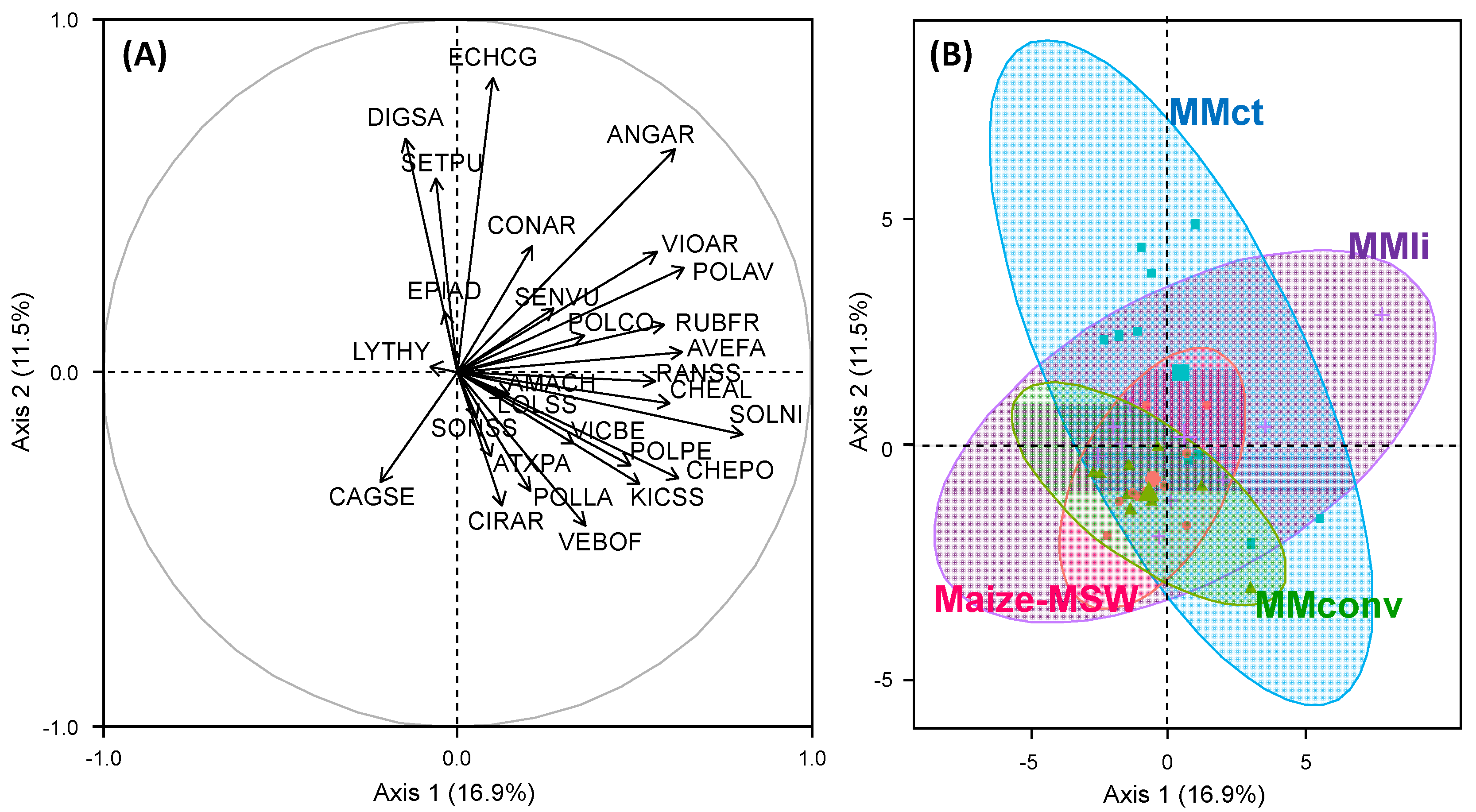
3.1. Effect of Cropping Systems on Weed Communities

The first and second axis of the PCA accounted for 16.9% and 11.5% of the total variance, respectively (Figure 1A). Three weed species contributed the most to the first axis: Solanum nigrum L. (14%), Polygonum aviculare L. (9%) and Avena fatua L. (9%). Echinochloa crus-galli (L.) P.Beauv. (22%), Digitaria sanguinalis (L.) Scop. (14%) and Lysimachia arvensis (L.) U.Manns & Anderb. (13%) contributed the most to the second axis. MM_Conv and Maize-MSW were associated with a low abundance of each weed species and a stable weed community across observations (Figure 1B). Observations corresponding to MM_LI are scattered, indicating a variable weed community and a higher species diversity across observations. MM_CT was associated with a greater presence of Digitaria sanguinalis (L.) Scop. and Echinochloa crus-galli (L.) P.Beauv. and a high variability across observations.

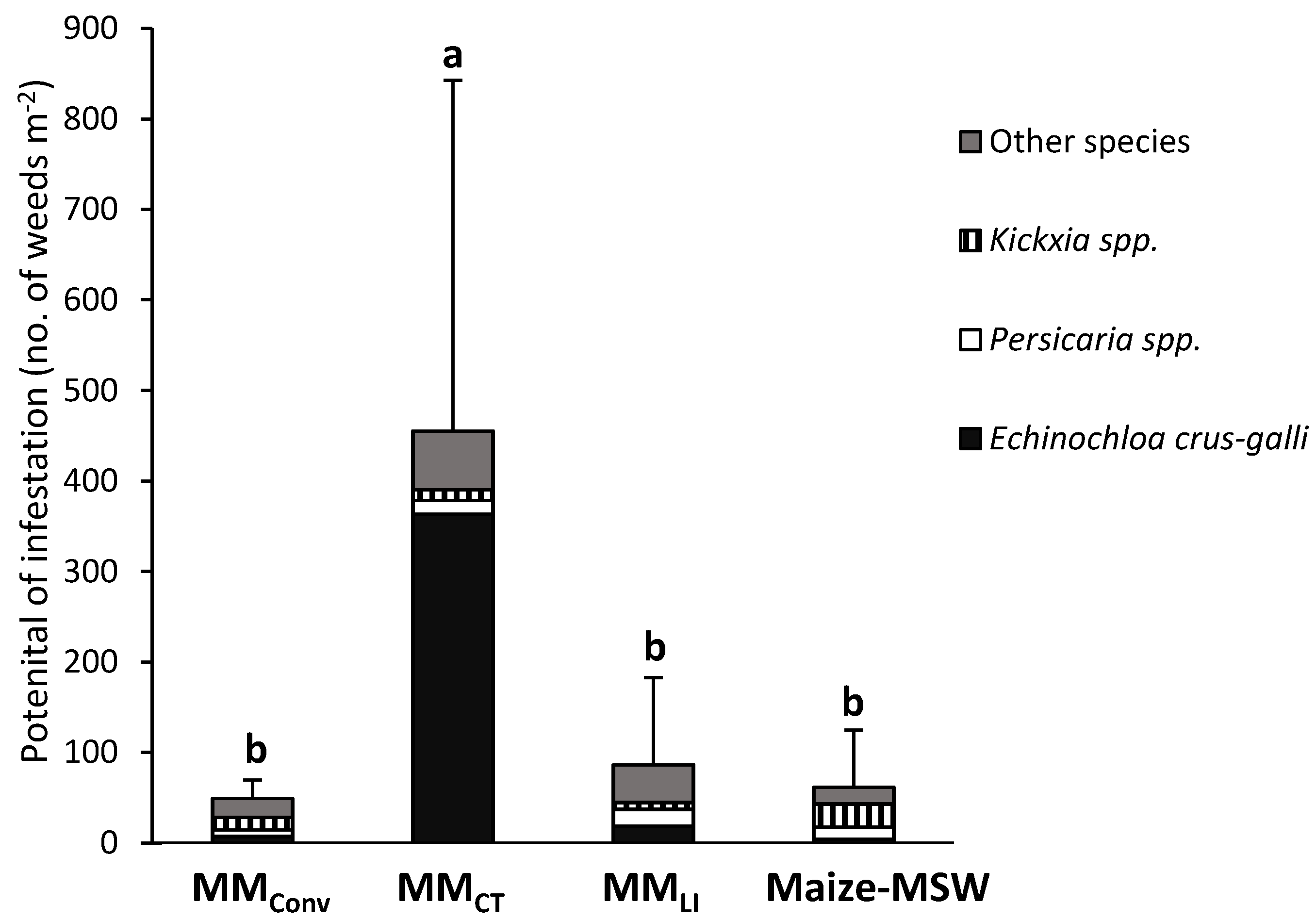
3.2. Potential of Infestation

Over the five-year experiment, system had a significant effect (p < 0.001) on mean PI (Figure 2). The mean (±standard deviation) PI of MM_CT (455 ± 387 plants m⁻²) was significantly greater than the mean PI of MM_Conv (49 ± 20 plants m⁻²), MM_LI (86 ± 97 plants m⁻²) and Maize-MSW (62 ± 63 plants m⁻²). PI in MM_Conv remained low and constant. MM_LI also showed a low PI although more variable than MM_Conv. MM_Conv and MM_LI presented similar weed communities with 15–21% of Echinochloa crus-galli (L.) P.Beauv. and 15–22% of Persicaria spp. The mean PI in MM_CT differed greatly from those in two other MM and was dominated by Echinochloa crus-galli (L.) P.Beauv. (80%). Mean PI in Maize-MSW was low and essentially represented by Kickxia spp. (41%) and Persicaria spp. (22%).

Significant differences of weed species PI were observed among the cropping systems (

Table 1. Weed species’ potential of infestation (mean ± standard deviation, no. of plants m⁻²) of the four cropping systems (MM_Conv: conventional maize monoculture; MM_CT: conservation tillage maize monoculture; MM_LI: low-input maize monoculture; Maize-MSW: integrated maize rotation). For each weed species, mean values sharing the same letter (“a” and/or “b”) are not different according to Tukey’s HSD test (denoted with ⁺) or Kruskal-Wallis test (denoted with ^‡) (** p < 0.01, *** p < 0.001).

Cropping System	Weed Species
	Convolvulus arvensis L. ‡		Digitaria sanguinalis (L.) Scop. ‡		Echinochloa crus-galli (L.) P.Beauv. +
MMConv	2 ± 2	b	0 ± 0	b	7 ± 7	b
MMCT	17 ± 7	a	13 ± 29	a	364 ± 399	a
MMLI	2 ± 2	b	1 ± 1	ab	18 ± 26	ab
Maize-MSW	2 ± 2	b	0 ± 0	b	4 ± 6	b
Significance p		***		**		***

). PI of Echinochloa crus-galli (L.) P.Beauv. (p < 0.001) and Digitaria sanguinalis (L.) Scop. (p < 0.01) were found at greater densities in MM_CT (363 ± 399 plants m⁻² and 13 ± 29 plants m⁻², respectively) than in MM_Conv (7 ± 7 plants m⁻² and 0 ± 0 plants m⁻², respectively). PI of Convolvulus arvensis L. (p < 0.001) was greater in MM_CT (17 ± 7 plants m⁻²) than in MM_Conv (2 ± 2 plants m⁻²).

3.3. Weed Population Dynamics

Mixed models were fitted to determine if PI of weed species in a given cropping system evolved significantly during the experiment. Total PI evolved significantly only in MM_CT, increasing from 74 ± 39 plants m⁻² in 2011 to 1008 ± 203 plants m⁻² in 2015.

Two significant positive evolutions were found according to species-by-species analysis in MM_CT (

Table 2. Evolution of the potential of infestation (PI, log10 transformed) with time (5 years of experiment) for each weed species in each cropping system (10 observations for each system over the 5-year experiment; MM_Conv: conventional maize monoculture; MM_CT: conservation tillage maize monoculture; MM_LI: low-input maize monoculture). Values represent the slope between time and weed species’ PI (log10 transformed) in the different cropping systems. Block was treated as a random factor. Slopes were tested to significantly different from zero (* p < 0.05, ** p < 0.01, *** p < 0.001, NA: not applicable, ns: not significant).

Cropping System	Weed Species
	Convolvulus arvensis L.	Digitaria sanguinalis (L.) Scop.	Echinochloa crus-galli (L.) P.Beauv.	Total
MMConv	−0.37 **	NA	ns	ns
MMCT	ns	0.66 *	1.37 **	0.66 ***
MMLI	ns	ns	ns	ns

): Echinochloa crus-galli (L.) P.Beauv. (from 3 ± 1 plants m⁻² in 2011 to 935 ± 218 plants m⁻² in 2015) and Digitaria sanguinalis (L.) Scop. (from 0 ± 0 plants m⁻² in 2011 to 15 ± 18 plants m⁻² in 2015). One significant negative evolution was found for a species with low PI: Convolvulus arvensis L. in MM_Conv (from 5 ± 1 plants m⁻² in 2011 to 0 ± 0 plants m⁻² in 2015).

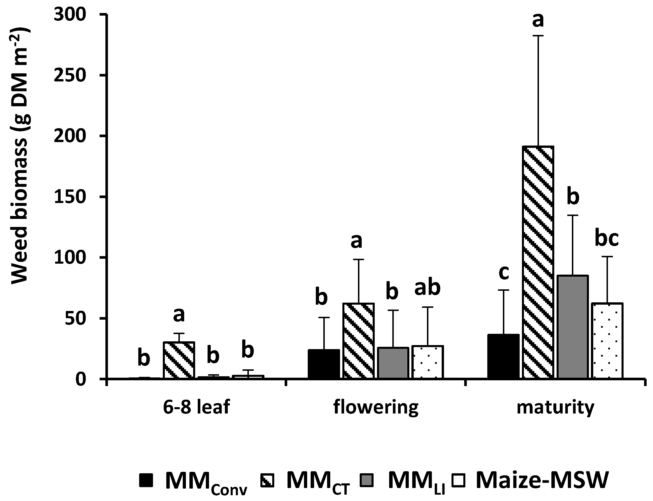
3.4. Weed Biomass: Effect of Cropping Systems at Different Maize Growth Stages

At the three sampling dates of maize (6–8 leaf, flowering, maturity), weed biomass was greater in MM_CT than in the other cropping systems, except Maize-MSW at flowering (Figure 3). At maize maturity, mean weed biomass in MM_LI (85 ± 50 g DM m⁻²) was significantly greater than in MM_Conv (36 ± 37 g DM m⁻²). At maturity, Maize-MSW weed biomass (62 ± 39 g DM m⁻²) was not statistically different from MM_LI and MM_Conv.

Significant differences in mean weed species biomass were observed among the cropping systems at maize maturity (2011–2015) (

Table 3. Biomass of weed species (mean ± standard deviation, g DM m⁻²) between the cropping systems (MM_Conv: conventional maize monoculture; MM_CT: conservation tillage maize monoculture; MM_LI: low-input maize monoculture; Maize-MSW: integrated maize rotation) at maize maturity (140–179 days after sowing). For each weed species, mean values followed by a same letter (“a” and/or “b”) are not different according to Tukey’s HSD test (denoted with °) or, when ANOVA assumptions were not met, the Kruskal-Wallis test (denoted with ^‡) (* p < 0.05, ** p < 0.01, *** p < 0.001).

Cropping System	Weed Species
	Chenopodium spp. ‡		Convolvulus arvensis L. ‡		Digitaria sanguinalis (L) Scop. ‡		Echinochloa crus-galli (L.) P.Beauv. °		Persicaria spp. °		Setaria pumila (Poir.) Roem. & Schult ‡
MMConv	1 ± 3	ab	1 ± 1	b	0	b	6 ± 7	b	17 ± 35	b	0 ± 0	ab
MMCT	1 ± 3	ab	4 ± 3	a	4 ± 6	a	140 ± 114	a	19 ± 2 6	ab	3 ± 5	a
MMLI	4 ± 5	a	2 ± 3	ab	1 ± 1	ab	25 ± 29	ab	31 ± 42	ab	0	b
Maize-MSW	0 ± 0	b	2 ± 3	ab	0 ± 0	b	14 ± 21	b	35 ± 41	a	0 ± 0	ab
Significance p		*		**		**		***		*		*

). Persicaria spp. biomass was greater in Maize-MSW (35 ± 41 g DM m⁻²) than MM_Conv (17 ± 35 g DM m⁻²) (p < 0.05). The biomass of Echinochloa crus-galli (L.) P.Beauv. (p < 0.001) was greater in MM_CT (140 ± 114 g DM m⁻²) than in MM_Conv (6 ± 7 g DM m⁻²).

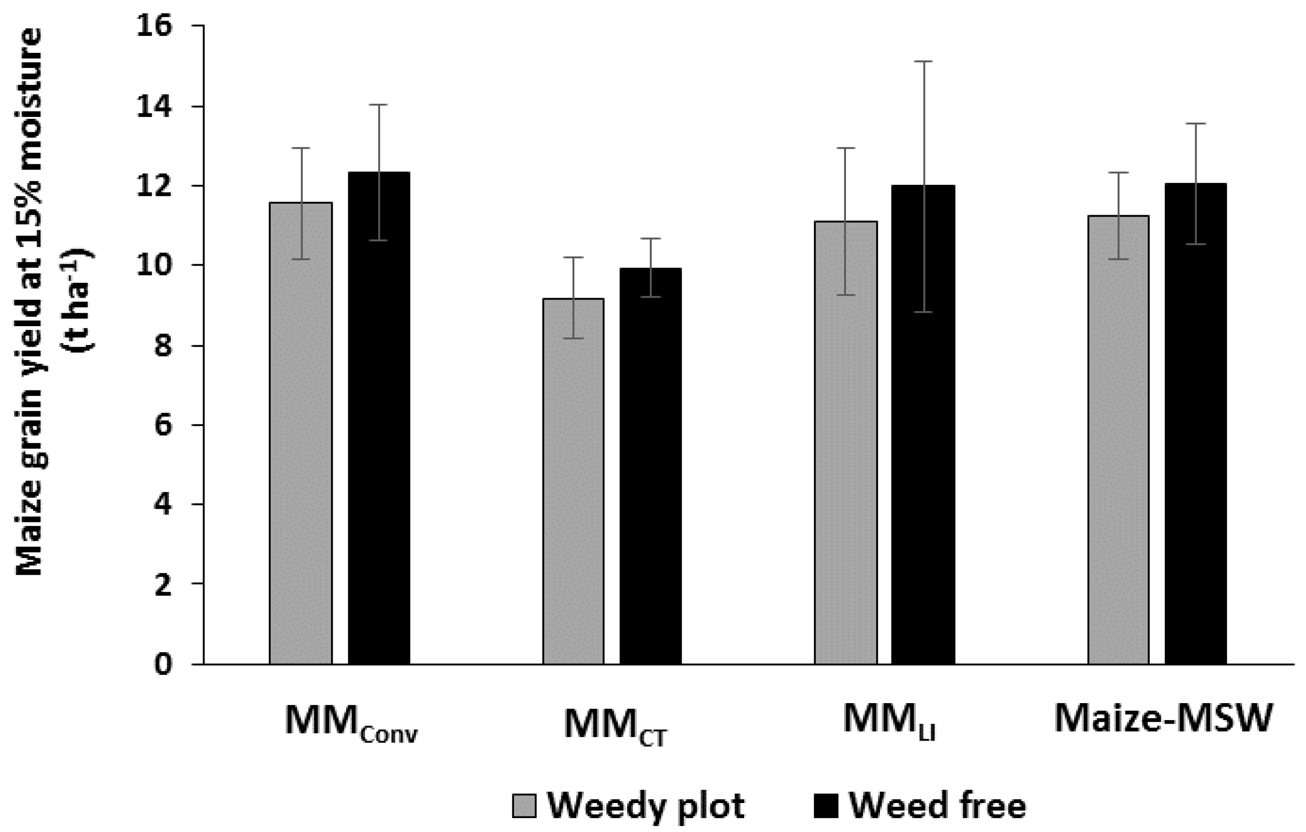
3.5. Impact of Weeds and Cropping Systems on Maize Yields

Cropping system had a significant effect (p < 0.001) on maize grain yields. Maize grain yields (

Table 4. Mean maize grain yield (mean ± standard deviation, at 15% moisture content, t ha⁻¹) of the cropping systems (MM_Conv: conventional maize monoculture; MM_CT: conservation tillage maize monoculture; MM_LI: low-input maize monoculture; Maize-MSW: integrated maize rotation). For each cropping system, mean values followed by the same letter (“a” and/or “b”) are not different according to Tukey’s HSD test (p < 0.05).

Cropping System	Year					Mean Yield
	2011	2012	2013	2014	2015
MMConv	10.8 ± 1.1	11.5 ± 1.3	10.9 ± 0.2	11.7 ± 2.2	11.4 ± 1.0	11.3 ± 1.1	a
MMCT	10.0 ± 1.3	6.6 ± 0.8	5.9 ± 0.4	8.5 ± 1.1	9.8 ± 0.4	8.2 ± 1.8	b
MMLI	10.0 ± 1.3	11.5 ± 1.7	7.8 ± 2.8	11.8 ± 2.1	10.3 ± 1.8	10.6 ± 2.3	a
Maize-MSW	9.4 ± 0.6	10.2 ± 1.6	6.4 ± 0.5	10.3 ± 0.1	12.2 ± 0.3	9.7 ± 2.1	ab

) were greater in MM_Conv (11.3 ± 1.1 t ha⁻¹) and MM_LI (10.6 ± 2.3 t ha⁻¹) than in MM_CT (8.2 ± 1.9 t ha⁻¹) and were not different from the three latter in Maize-MSW (9.7 ± 2.0 t ha⁻¹). Yield variability was greater in all three low-input cropping systems, particularly due to waterlogging that led to lower yields in 2013 (MM_LI: 7.8 ± 2.8 t ha⁻¹; MM_CT: 5.9 ± 0.4 t ha⁻¹, Maize-MSW: 6.5 ± 0.5 t ha⁻¹) than those in MM_Conv (10.9 ± 2.1 t ha⁻¹), which was the only system ploughed that year.

The analysis between cropping system and weed biomass at maize maturity revealed an effect of cropping system (p < 0.001; Intercept (t ha⁻¹): MM_Conv (11.7), MM_LI (11.3), MM_CT (10.3), Maize-MSW (10.4)) and biomass (p < 0.01; Slope = −1.1) on yield but did not reveal an interaction between the two factors (p = 0.29), indicating that the relationship between weed biomass and yield did not differ among cropping systems.

The analysis of weed free zones revealed a hand weeding (yes/no) effect (p < 0.05) on yield but no system effect (p = 0.19) or interaction (p = 0.99), indicating that weeds present after management generated similar yield losses among the four cropping systems in 2014 and 2015 (Figure 4), despite different weed biomasses. Across all four systems, yields in hand weeded plots (11.6 ± 2.0 t ha⁻¹) were significantly greater than yields in plots without supplemental hand weeding (10.7 ± 1.6 t ha⁻¹).

4. Discussion

4.1. Efficient Weed Management in Low-Input Cropping Systems

During this five-year experiment, MM_Conv achieved a high and consistent yield and was associated with low weed density and biomass. These results confirm, via a cropping system approach, that the decision rules and resulting weeding and farming practices were sufficient to ensure the economic viability of this cropping system [42]. The combination of farming practices, such as annual mouldboard ploughing [49], systematic use of pre-emergence herbicides [50] followed by one or two remedial sprays [51], techniques known to be efficient weed-management tools, provided acceptable weed control and achieved high yields. However, this reference cropping system is challenged by the environmental and long-term risks it generates, such as soil erosion due to bare soil during the winter [4], herbicide resistance [3], high pesticide leaching [52] and high greenhouse gas emissions, the former two being confirmed by results collected on that experiment [42].

MM_LI was also a high-yielding cropping system although more variable than MM_Conv, based on the standard deviations. PI was also more variable than in the reference system (MM_Conv). Differences between these two cropping systems are not as large when one compares weed biomasses – an integrative indicator to measure weed pressure [53]. MM_LI’s weeding strategy (pre-emergence soil-applied herbicides on the row combined with cultivation later in the season) can temporarily lead to high weed density and thus, PI because of the absence of weeding operations in the inter-row early in the season. Yet, weed biomass at maize flowering did not differ between MM_Conv and MM_LI because the late inter-row mechanical weeding operations, occasionally paired with chemical sprays on the rows, effectively controlled weeds [18].

Despite differences in weed management, both cropping systems generated similar weed communities. The main weed species were annual summer grasses such as Echinochloa crus-galli (L.) P.Beauv., and annual spring/summer forbs such as Persicaria spp. and Kickxia spp., all species particular adapted to conventionally-tilled maize-based crop rotations [11]. Moreover, MM_Conv reduced the presence of Convolvulus arvensis L., which is consistent with previous studies [54].

4.2. Conservation Tillage

MM_CT showed lower and more variable maize yields than MM_Conv. Yields were particularly reduced in 2012 and 2013, which were the second and third year after the transition to conservation tillage, respectively, which illustrates the complicated transition phase often mentioned for these cropping systems [55] and the importance of implementing rotation as a weed management tool in conservation agriculture [56]. These poor performances can also be the result of an abrupt transition from annual tillage to no-till without enough time in between for cover crops and organisms to biologically restructure the soil and reorganise soil organic matter (which was low ~2%). Reduced maize yields under conservation tillage have been noted in other studies [57] but are not consistent across the world [58] according to the pedo-climatic conditions and the cropping system studied.

MM_CT required greater herbicide use to compensate for the absence of ploughing, mechanical weeding techniques and pre-emergence herbicides, i.e., S-metolachlor, which were abandoned in 2014 in this system because of reduced effectiveness due to surface mulch effect (see Figure S4 for data on cover crop biomass for all systems). However, in conservation agriculture, greater herbicide use during the transition phase could be counterbalanced in time by reduced herbicide use (if weeds are well managed and the superficial weed seed bank is depleted), reduced soil erosion, greater carbon sequestration and soil fertility [56]. Higher weed infestation has been observed in conservation tillage agriculture [54] and if weeds are not well managed, like Echinochloa crus-galli (L.) P.Beauv. in MM_CT which reached maturity at high densities (see Table S3 for list of species observed with mature or immature seeds at maize maturity in the four cropping systems), they can replenish the weed seedbank and create challenges for weed management over the long term. However, it is not always observed [12] because weed emergence is reduced when seeds remain on the soil surface as in zero-tillage systems [30]. Indeed, under these conditions seed-soil contact is poor and seeds are exposed to light [59].

Along with higher weed pressure, the weed community in MM_CT shifted towards annual grasses (Echinochloa crus-galli (L.) P.Beauv., Digitaria sanguinalis (L.) Scop. and Setaria pumila (Poir.) Roem. & Schult.), which completely dominated after the first two years of the experiment, as reported in previous studies [4]. Grasses are adapted to conservation agriculture because no-till maintains weed seeds on the soil surface, where annual grass seeds are able to germinate [30]. Convolvulus arvensis L., a geophyte perennial broadleaf, most likely benefited from this system due to minimal soil disturbance [11].

4.3. Rotating Maize

Maize yields were quite high in the MSW cropping system and were similar to those of MM_LI and MM_Conv if one ignores 2013, the year both plots in this system were flooded for two months after sowing. Even though the literature emphasises that crop rotation increases maize yield [60], this was not the case in this experiment. This is most likely because, here, maize management in the rotation differed from that in the reference monoculture (MM_Conv): reduced N fertilization, irrigation and chemical sprays. However, in 2015, Maize-MSW was the highest yielding cropping system with 12.2 ± 0.3 t ha⁻¹. This suggests that low-input cropping systems with diversified rotations could generate long term high crop performance along with environmental benefits (water quality and quantity, energy use).

Maize-MSW had a low HTFI because of the efficiency of the main agronomic tools implemented: rotation [7], mouldboard ploughing before maize [54], mechanical weeding [61] and chemical spraying centred on the crop row [18]. Moreover, it obtained good results for all weed-management indicators: PI and weed biomass were similar to those of MM_Conv and slightly reduced compared to MM_LI, which used a similar strategy to manage the crop, minus crop rotation. Moreover, even though not significantly different, the PI of Echinochloa crus-galli (L.) P.Beauv., the most important weed of the experiment, was 4.5 times lower in Maize-MSW than in MM_LI, indicating that rotating maize with winter (e.g., wheat) and/or dicotyledonous (e.g., soybean) cash crops could negatively affect this noxious summer germinating grass species [8,62]. This is in accordance with [63], who reported that Echinochloa crus-galli (L.) P.Beauv. was found in greater proportions in monocultured plots than in plots in rotation, possibly due to loss of seed viability during the winter crop phase of the rotation. Finally, even though their percentages differed, the main weed species were similar in Maize-MSW, MM_Conv and MM_LI. It can be hypothesised that, for a given crop type, mouldboard ploughing influences weed composition more than all other techniques used to manage weeds, including crop rotation as suggested by Fried et al. [7].

4.4. Weed Biomass at Maturity and Maize Yield

Even though studies show that the critical period of maize:weed competition extends from sowing to the 3–6 leaf stage [64] or the 3–14 leaf stage [65], weed biomass at maize maturity had the highest correlation with maize grain yield. It is most likely that weed biomass at maize maturity integrates the effect of competition between maize and weeds during the entire crop cycle.

More interestingly, the statistical analysis did not reveal significantly different slopes among cropping systems for the effect of weed biomass on maize yield (2011–2015). Since external outputs such as fertilization and irrigation were more important in MM_Conv, a reduced impact of weed biomass on maize yields could have been expected in this cropping system.

In contrast, the analysis of weed free zones (2014–2015) showed that weed biomass, even though variable across the cropping systems (at maize maturity: 17 ± 17 g DM m⁻² in MM_Conv, 209 ± 71 g DM m⁻² in MM_CT, 72 ± 54 g DM m⁻² in MM_LI and 24 ± 9 g DM m⁻² in Maize-MSW), did not significantly affect yields differently across the cropping systems (yield losses varying from 0.7 to 0.9 t ha⁻¹). This suggests that weeds (in 2014 and 2015) were managed as well in the low input cropping systems as in the reference system, mainly because of a delayed emergence with respect to the crop. However, an important yield gap exists between MM_CT and the three other cropping systems in weed-free zones (2.1 t ha⁻¹ in average). Hence, we can hypothesize that, in this experiment, the influence of soil properties (linked to no-tillage) on maize grain yields was greater than the impact of weed pressure, at least in the context of non-limiting resources. However, it is important to note that maize yields could also have been influenced by other factors that differed among the cropping systems, such as planting date (MM_CT), choice of cultivars and fertilization (low-input cropping systems). Maize pests and diseases were adequately managed in all plots throughout the experiment.

5. Conclusions

This maize-based cropping system experiment demonstrated that two of three innovative cropping systems which implemented various techniques (such as mechanical weeding, mixed weeding, cover-crop introduction, reduced inputs, and crop rotation) had the same weed management success (in terms of PI and biomass) as the reference system and that weed communities and yields did not drastically differ from the latter, although more variable in MM_LI. The overall impact of weeds on maize performance was limited because weeds were well managed, except in the MM_CT which selected grasses and perennials (higher PI and weed biomasses at maturity). The absence of significant yield difference between the field and the weed free zones indicate that lower maize yield in conservation tillage could not be attributed to higher weed pressure, even though the latter was higher than in the other systems. Overall, weed biomasses and PI show that IWM cropping systems are efficient at properly managing weeds while maintaining grain yield and should provide insight on how maize farmers can innovate their cropping systems to maximize environmental benefits without fearing low agronomic performance. However, the adoption of these CS to farmers in South-Western France questions the ability of these system to be managed at wider temporal and spatial scales.

References

1. Bosnic, A.C.; Swanton, C.J. Influence of barnyardgrass (Echinochloa. crus-galli) time of emergence and density on corn (Zea mays). Weed Sci. 1997, 45, 276–282. [Google Scholar] [CrossRef]
2. Aymard, D.; Cassagne, J.P.; Sablik, M.C. Mémento Agricole du Bassin Adour-Garonne; Ministère de L’agriculture, Agro-Alimentaire et de la Forêt: Paris, France, 2014. [Google Scholar]
3. Heap, I. Herbicide resistant weeds. In Integrated Pest Management; Springer: Dordrecht, The Netherlands, 2014; pp. 281–301. [Google Scholar]
4. Stoate, C.; Boatman, N.D.; Borralho, R.J.; Carvalho, C.R.; Snoo, G.R.D.; Eden, P. Ecological impacts of arable intensification in Europe. J. Environ. Manag. 2001, 63, 337–365. [Google Scholar] [CrossRef]
5. Chikowo, R.; Faloya, V.; Petit, S.; Munier-Jolain, N.M. Integrated weed management systems allow reduced reliance on herbicides and long-term weed control. Agric. Ecosyst. Environ. 2009, 132, 237–242. [Google Scholar] [CrossRef]
6. Liebman, M.; Gallandt, E.R. Many little hammers: Ecological management of crop-weed interactions. In Ecology in Agriculture; Academic Press: San Diego, CA, USA, 1997; pp. 291–343. [Google Scholar]
7. Fried, G.; Norton, L.R.; Reboud, X. Environmental and management factors determining weed species composition and diversity in France. Agric. Ecosyst. Environ. 2008, 128, 68–76. [Google Scholar] [CrossRef]
8. Chauvel, B.; Guillemin, J.; Colbach, N.; Gasquez, J. Evaluation of cropping systems for management of herbicide-resistant populations of blackgrass (Alopecurus. myosuroides Huds.). Crop Prot. 2001, 20, 127–137. [Google Scholar] [CrossRef]
9. Booth, B.D.; Swanton, C.J. Assembly theory applied to weed communities. Weed Sci. 2002, 50, 2–13. [Google Scholar] [CrossRef]
10. Morris, N.; Miller, P.; Orson, J.; Froud-Williams, R. The adoption of non-inversion tillage systems in the United Kingdom and the agronomic impact on soil, crops and the environment—A review. Soil Tillage Res. 2010, 108, 1–15. [Google Scholar] [CrossRef]
11. Zanin, G.; Otto, S.; Riello, L.; Borin, M. Ecological interpretation of weed flora dynamics under different tillage systems. Agric. Ecosyst. Environ. 1997, 66, 177–188. [Google Scholar] [CrossRef]
12. Murphy, S.D.; Clements, D.R.; Belaoussoff, S.; Kevan, P.G.; Swanton, C.J. Promotion of weed species diversity and reduction of weed seedbanks with conservation tillage and crop rotation. Weed Sci. 2006, 54, 69–77. [Google Scholar] [CrossRef]
13. O’Connell, P.J.; Harms, C.T.; Allen, J.R. Metolachlor, S-metolachlor and their role within sustainable weed-management. Crop Prot. 1998, 17, 207–212. [Google Scholar] [CrossRef]
14. Dobbels, A.F.; Kapusta, G. Postemergence weed control in corn (Zea mays) with nicosulfuron combinations. Weed Technol. 1993, 7, 844–850. [Google Scholar] [CrossRef]
15. Johnson, B.C.; Young, B.G.; Matthews, J.L. Effect of postemergence application rate and timing of mesotrione on corn (Zea mays) response and weed control. Weed Technol. 2002, 16, 414–420. [Google Scholar] [CrossRef]
16. Spaunhorst, D.J.; Bradley, K.W. Influence of dicamba and dicamba plus glyphosate combinations on the control of glyphosate-resistant waterhemp (Amaranthus. rudis). Weed Technol. 2013, 27, 675–681. [Google Scholar] [CrossRef]
17. Riemens, M.; Van Der Weide, R.; Bleeker, P.; Lotz, L. Effect of stale seedbed preparations and subsequent weed control in lettuce (cv. Iceboll) on weed densities. Weed Res. 2007, 47, 149–156. [Google Scholar] [CrossRef]
18. Leblanc, M.L.; Cloutier, D.C.; Leroux, G.D. Réduction de l’utilisation des herbicides dans le maïs-grain par une application d’herbicides en bandes combinée à des sarclages mécaniques. Weed Res. 1995, 35, 511–522. [Google Scholar] [CrossRef]
19. Henson, I. The effects of light, potassium nitrate and temperature on the germination of Chenopodium album. Weed Res. 1970, 10, 27–39. [Google Scholar] [CrossRef]
20. Espeby, L. Germination of Weed Seeds and Competition in Stands of Weeds and Barley: Influences of Mineral Nutrients; Department of Crop Production Science, Swedish University of Agricultural Sciences: Uppsala, Sweden, 1989. [Google Scholar]
21. Fawcett, R.; Slife, F. Effects of field applications of nitrate on weed seed germination and dormancy. Weed Sci. 1978, 26, 594–596. [Google Scholar] [CrossRef]
22. Banks, P.; Santelmann, P.; Tucker, B. Influence of long-term soil fertility treatments on weed species in winter wheat. Agron. J. 1976, 68, 825–827. [Google Scholar] [CrossRef]
23. Dyck, E.; Liebman, M. Soil fertility management as a factor in weed control: The effect of crimson clover residue, synthetic nitrogen fertilizer, and their interaction on emergence and early growth of lambsquarters and sweet corn. Plant Soil 1994, 167, 227–237. [Google Scholar] [CrossRef]
24. Jørnsgård, B.; Rasmussen, K.; Hill, J.; Christiansen, J.L. Influence of nitrogen on competition between cereals and their natural weed populations. Weed Res. 1996, 36, 461–470. [Google Scholar] [CrossRef]
25. Pyšek, P.; Lepš, J. Response of a weed community to nitrogen fertilization: A multivariate analysis. J. Veg. Sci. 1991, 2, 237–244. [Google Scholar] [CrossRef]
26. O’Donovan, J.T.; McAndrew, D.W.; Thomas, A.G. Tillage and nitrogen influence weed population dynamics in barley (Hordeum. vulgare). Weed Technol. 1997, 11, 502–509. [Google Scholar] [CrossRef]
27. Pawar, L.; Yaduraju, N.; Ahuja, K. Population dynamics of weeds and their growth in tall and dwarf wheat as influenced by sub-optimal levels of irrigation and nitrogen. Indian J. Ecol. 1998, 25, 146–154. [Google Scholar]
28. Andersson, T.N.; Milberg, P. Weed Flora and the Relative Importance of Site, Crop, Crop Rotation, and Nitrogen. Weed Sci. 1998, 46, 30–38. Available online: http://www.jstor.org/stable/4046005 (accessed on 8 January 2017).
29. Blackshaw, R.E.; Molnar, L.J.; Janzen, H.H. Nitrogen fertilizer timing and application method affect weed growth and competition with spring wheat. Weed Sci. 2004, 52, 614–622. [Google Scholar] [CrossRef]
30. Cordeau, S.; Guillemin, J.-P.; Reibel, C.; Chauvel, B. Weed species differ in their ability to emerge in no-till systems that include cover crops. Ann. Appl. Biol. 2015, 166, 444–455. [Google Scholar] [CrossRef]
31. Brennan, E.B.; Smith, R.F. Winter cover crop growth and weed suppression on the central coast of California. Weed Technol. 2005, 19, 1017–1024. [Google Scholar] [CrossRef]
32. Yeganehpoor, F.; Salmasi, S.Z.; Abedi, G.; Samadiyan, F.; Beyginiya, V. Effects of cover crops and weed management on corn yield. J. Saudi Soc. Agric. Sci. 2015, 14, 178–181. [Google Scholar] [CrossRef]
33. Teasdale, J.; Mohler, C. Light transmittance, soil temperature, and soil moisture under residue of hairy vetch and rye. Agron. J. 1993, 85, 673–680. [Google Scholar] [CrossRef]
34. Reddy, K.N.; Koger, C.H. Live and killed hairy vetch cover crop effects on weeds and yield in glyphosate-resistant corn. Weed Technol. 2004, 18, 835–840. [Google Scholar] [CrossRef]
35. Blackshaw, R.E.; Upadhyaya, M.K. Non-Chemical Weed Management: Principles, Concepts and Technology; Centre for Agriculture and Bioscience International: Oxfordshire, UK, 2007. [Google Scholar]
36. Blackshaw, R.E.; Moyer, J.R.; Doram, R.C.; Boswell, A.L. Yellow sweetclover, green manure, and its residues effectively suppress weeds during fallow. Weed Sci. 2001, 49, 406–413. [Google Scholar] [CrossRef]
37. Kunz, C.; Sturm, D.; Varnholt, D.; Walker, F.; Gerhards, R. Allelopathic effects and weed suppressive ability of cover crops. Plant Soil Environ. 2016, 62, 60–66. [Google Scholar] [CrossRef]
38. Tollenaar, M.; Aguilera, A.; Nissanka, S.P. Grain yield is reduced more by weed interference in an old than in a new maize hybrid. Agron. J. 1997, 89, 239–246. [Google Scholar] [CrossRef]
39. Derby, N.E.; Steele, D.D.; Terpstra, J.; Knighton, R.E.; Casey, F.X. Interactions of nitrogen, weather, soil, and irrigation on corn yield. Agron. J. 2005, 97, 1342–1351. [Google Scholar] [CrossRef]
40. Gholamhoseini, M.; AghaAlikhani, M.; Modarres Sanavy, S.A.M.; Mirlatifi, S.M. Interactions of irrigation, weed and nitrogen on corn yield, nitrogen use efficiency and nitrate leaching. Agric. Water Manag. 2013, 126, 9–18. [Google Scholar] [CrossRef]
41. Das, T.; Yaduraju, N. Effect of weed competition on growth, nutrient uptake and yield of wheat as affected by irrigation and fertilizers. J. Agric. Sci. 1999, 133, 45–51. [Google Scholar] [CrossRef]
42. Giuliano, S.; Ryan, M.R.; Véricel, G.; Rametti, G.; Perdrieux, F.; Justes, E.; Alletto, L. Low-input cropping systems to reduce input dependency and environmental impacts in maize production: A multi-criteria assessment. Eur. J. Agron. 2016, 76, 160–175. [Google Scholar] [CrossRef]
43. IUSS Working Group WRB. World Reference Base for Soil Resources 2006; First Update 2007; Food and Agriculture Organization (FAO): Rome, Italy, 2007. [Google Scholar]
44. Organisation for Economic Co-operation and Development. Environmental indicators for agriculture. In Methods and Results; OECD Publications: Paris, France, 2001; Volume 3. [Google Scholar]
45. Cordeau, S.; Dessaint, F.; Munier-Jolain, N.M. Long-term assessment of integrated weed management cropping systems in France. Asp. Appl. Biol. 2015, 128, 275–278. [Google Scholar]
46. Stoller, E.W.; Wax, L.M. Periodicity of germination and emergence of some annual weeds. Weed Sci. 1973, 21, 574–580. [Google Scholar] [CrossRef]
47. Hughes, G. The problem of weed patchiness. Weed Res. 1990, 30, 223–224. [Google Scholar] [CrossRef]
48. R Development Core Team. R: A Language and Environment for Statistical Computing; The R Foundation for Statistical Computing: Vienna, Austria, 2011. [Google Scholar]
49. Roger-Estrade, J.; Colbach, N.; Leterme, P.; Richard, G.; Caneill, J. Modelling vertical and lateral weed seed movements during mouldboard ploughing with a skim-coulter. Soil Tillage Res. 2001, 63, 35–49. [Google Scholar] [CrossRef]
50. Pannacci, E.; Graziani, F.; Covarelli, G. Use of herbicide mixtures for pre and post-emergence weed control in sunflower (Helianthus annuus). Crop Prot. 2007, 26, 1150–1157. [Google Scholar] [CrossRef]
51. Streit, B.; Rieger, S.B.; Stamp, P.; Richner, W. The effect of tillage intensity and time of herbicide application on weed communities and populations in maize in central Europe. Agric. Ecosyst. Environ. 2002, 92, 221–224. [Google Scholar] [CrossRef]
52. Alletto, L.; Giuliano, S.; Perdrieux, F.; Rametti, G.; Benoit, P.; Véricel, G.; Justes, E. Comparison of the environmental performances of four maize monocropping systems: A three years monitoring of pesticides leaching. In Proceedings of the Pesticide Behaviour in Soils, Water and Air Conference, York, North Yorkshire, UK, 2–4 September 2013. [Google Scholar]
53. Primot, S.; Valantin-Morison, M.; Makowski, D. Predicting the risk of weed infestation in winter oilseed rape crops. Weed Res. 2006, 46, 22–33. [Google Scholar] [CrossRef]
54. Buhler, D.D.; Stoltenberg, D.E.; Becker, R.L.; Gunsolus, J.L. Perennial weed populations after 14 years of variable tillage and cropping practices. Weed Sci. 1994, 42, 205–209. [Google Scholar] [CrossRef]
55. Odhiambo, J.A.; Norton, U.; Ashilenje, D.; Omondi, E.C.; Norton, J.B. Weed dynamics during transition to conservation agriculture in western Kenya maize production. PLoS ONE 2015, 10, e0133976. [Google Scholar] [CrossRef] [PubMed]
56. Chauhan, B.S.; Singh, R.G.; Mahajan, G. Ecology and management of weeds under conservation agriculture: A review. Crop Prot. 2012, 38, 57–65. [Google Scholar] [CrossRef]
57. Van den Putte, A.; Govers, G.; Diels, J.; Gillijns, K.; Demuzere, M. Assessing the effect of soil tillage on crop growth: A meta-regression analysis on European crop yields under conservation agriculture. Eur. J. Agron. 2010, 33, 231–241. [Google Scholar] [CrossRef]
58. Pittelkow, C.M.; Liang, X.; Linquist, B.A.; Van Groenigen, K.J.; Lee, J.; Lundy, M.E.; van Gestel, N.; Six, J.; Venterea, R.T.; van Kessel, C. Productivity limits and potentials of the principles of conservation agriculture. Nature 2015, 517, 365–368. [Google Scholar] [CrossRef] [PubMed]
59. Chauhan, B.S.; Johnson, D.E. The role of seed ecology in improving weed management strategies in the tropics. Adv. Agron. 2010, 105, 221–262. [Google Scholar] [CrossRef]
60. Bullock, D.G. Crop rotation. Crit. Rev. Plant Sci. 1992, 11, 309–326. [Google Scholar] [CrossRef]
61. Van Der Weide, R.Y.; Bleeker, P.O.; Achten, V.T.J.M.; Lotz, L.A.P.; Fogelberg, F.; Melander, B. Innovation in mechanical weed control in crop rows. Weed Res. 2008, 48, 215–224. [Google Scholar] [CrossRef]
62. Kropff, M.; Vossen, F.; Spitters, C.; De Groot, W. Competition between a maize crop and a natural population of Echinochloa crus-galli (L.) Pb. Neth. J. Agric. Sci. 1984, 32, 324–327. [Google Scholar]
63. Maun, M.; Barrett, S. The biology of Canadian weeds: 77. Echinochloa crus-galli (L.) Beauv. Can. J. Plant Sci. 1986, 66, 739–759. [Google Scholar] [CrossRef]
64. Hugo, E.; Morey, L.; Saayman-Du Toit, A.E.; Reinhardt, C.F. Critical periods of weed control for naked crabgrass (Digitaria nuda), a grass weed in corn in South Africa. Weed Sci. 2014, 62, 647–656. [Google Scholar] [CrossRef]
65. Hall, M.R.; Swanton, C.J.; Anderson, G.W. The critical period of weed control in grain corn (Zea mays). Weed Sci. 1992, 40, 441–447. [Google Scholar] [CrossRef]
Figure 1. (A) Correlation circle with the first two axes of principal component analysis (PCA) performed for the matrix of plots (N = 40, i.e., four cropping systems replicated twice over 5 years) and weed species (N = 28, described by the “Potential of Infestation” indicator). Weed species are indicated by their EPPO codes (http://eppt.eppo.org). Table S2 details the correspondance between the EPPO code and the species name. (B) Scatter diagram with the first two axes of the PCA. Ellipses represent a 95% confidence interval for each cropping system (MMConv: conventional maize monoculture; MMCT: conservation tillage maize monoculture; MMLI: low-input maize monoculture; Maize-MSW: integrated maize rotation).
Agriculture 07 00074 g001
Figure 2. Potential of infestation (PI, see equation for details) detailed for the three main weed species (mean values over the 5-year period, 2011–2015) in the four cropping systems (MMConv: conventional maize monoculture; MMCT: conservation tillage maize monoculture; MMLI: low-input maize monoculture; Maize-MSW: integrated maize rotation, N = 10 quadrats per cropping system). Year and block were treated as random factors. Error bars represent standard deviations. ANOVA tested a system effect p < 0.001). Bars sharing the same letter (“a” and/or ”b”) are not significantly different (p < 0.05, Tukey HSD Test).
Agriculture 07 00074 g002
Figure 3. Mean weed biomass at three stages of maize growth in the four cropping systems (MMConv: conventional maize monoculture; MMCT: conservation tillage maize monoculture; MMLI: low-input maize monoculture; Maize-MSW: integrated maize rotation). Weed biomass at the 6–8 leaf stage was sampled only in 2014 and 2015 (N = 4 quadrats per cropping system) whereas weed biomass at the flowering and maturity stage was sampled from 2011 to 2015 (N = 10 quadrats per cropping system). Year and block were treated as random factors. Error bars represent standard deviation. ANOVA tested for system effect (6–8 leaf: p < 0.001; Flowering: p = 0.01; Maturity: p < 0.001). Bars sharing the same letter (“a” and/or “b”, and/or “c”) within each crop stage are not significantly different (p < 0.05, Tukey HSD Test). Sampling (days after sowing): 8 leaf (48–58), flowering (76–113), maturity (140–179).
Agriculture 07 00074 g003
Figure 4. Mean maize grain yield (at 15% water content, t ha−1) in the presence or absence of weeds (weed-free zones, hand-weeded, N = 4 quadrats in each zone and cropping system) assessed in 2014 and 2015 for each cropping system (MMConv: conventional maize monoculture; MMCT: conservation tillage maize monoculture; MMLI: low-input maize monoculture; Maize-MSW: integrated maize rotation). Error bars represent standard deviations. ANOVA: hand weeding effect (p < 0.05); cropping system effect (non-significant).
Agriculture 07 00074 g004