Optimal Level of Woody Biomass Co-Firing with Coal Power Plant Considering Advanced Feedstock Logistics System

Abstract

Co-firing from woody biomass feedstock is one of the alternatives toward increased use of renewable feedstock in existing coal power plants. However, the economic level of co-firing at a particular power plant depends on several site-specific factors. Torrefaction has been identified recently as a promising biomass pretreatment option to lead to reduction of the feedstock delivered cost, and thus facilitate an increase in the co-firing ratio. In this study, a mixed integer linear program (MILP) is developed to integrate supply chain of co-firing and torrefaction process and find the optimal level of biomass co-firing in terms of minimized transportation and logistics costs, with or without tax credits. A case study of 26 existing coal power plants in three Great Lakes States of the US is used to test the model. The results reveal that torrefaction process can lead to higher levels of co-firing, but without the tax credit, the effect is limited to the low capacity of power plants. The sensitivity analysis shows that co-firing ratio has higher sensitivity to variation in capital and operation costs of torrefaction than to the variation in the transportation and feedstock purchase costs.

1. Introduction

1.1. Background and Research Objectives

Burning coal produces many gases and heavy metals, which affect the environment and human health [1]. The objective to reduce these effects has encouraged numerous policies to support the increasing generation of electricity with renewable energy resources. While many alternative technologies remain in the early-to-mid stages of development, co-firing is a mature solution to reduce ${\mathrm{CO}}_2$ emissions from coal power plants [2].

Many researches have addressed the attractive aspects of biomass co-firing [2,3,4]. First, it is known that net greenhouse effect of the biomass combustion is zero and it can contribute to reduced emissions, such as ${\mathrm{SO}}_2$ and ${\mathrm{NO}}_2$. Second, the biomass co-firing minimizes the environmental problems relating to agricultural waste and its disposal. Finally, the biomass co-firing does not require extensive capital investment. For example, if less than 4% fraction by mass in existing coal power plants is from biomass, it can be burned without a separate fuel feeding system [5].

However, there are several drawbacks of using biomass for power generation, such as the loss of boiler efficiency and high transportation costs for biomass feedstock. Boiler efficiency and performance can decrease, if proper design and operational changes are not considered [6]. In addition, biomass co-firing can increase both the high and low temperature corrosion rate in utility boilers, as the properties of biomass feedstock differ significantly from coal [7]. For these reasons, the desired co-firing ratio should be determined based on several site-specific factors.

Economic impact of increased fuel volume required is another critical factor to consider. Transportation and logistics costs contribute to a large portion of total procurement costs for biomass feedstock. Biomass transportation is often considered a competitive, low-margin business, as the inherent features of the feedstock result in a low-efficiency transportation enterprise [8]. These features include a large number of points of origin for loads, often with limited accessibility, needs for specialized equipment that lessen opportunities for product backhauls, and a significant portion of operating hours spent loading and unloading the product [9].

Torrefaction has been identified as a promising biomass pretreatment option that can facilitate reduction of the feedstock delivered cost and thus allow increasing the co-firing ratio [10]. Torrefaction is a thermal treatment of biomass under atmospheric conditions without air or oxygen in the temperature range 250–300 °C. At optimum conditions, torrefied biomass has been found to contain 70–80% of the original mass while retaining 80–90% of original energy [11,12], thus torrefaction makes energy density per unit of mass increase by around 30%. In other words, torrefaction can change biomass properties and improve the fuel quality for combustion and gasification applications. At the same time, it can also create benefits through lower storage and transportation costs.

In this study, we develop mathematical model to integrate supply chain of co-firing and torrefaction process and find the optimal level of biomass co-firing in terms of minimized transportation and logistics costs. While there are several methods of co-firing, direct co-firing with the coal and biomass in the same boiler is used in this paper, as it is the simplest and most widely applied technology for biomass co-firing [7]. The main contributions of this research are as follows:

• We incorporate the torrefaction processing option in the estimation of optimized biomass co-firing ratio.
• We compare the conventional and advanced logistics to verify the most appropriate logistics system for biomass co-firing.
• We evaluate the proposed model through a case study for the Great Lakes States considering actual seasonal variations of biomass feedstock in study area.
• We compare the impacts of (1) the tax credit as a governmental incentive, and (2) selecting torrefaction process on the preferred level of biomass co-firing.

The remainder of the paper is divided into four sections. The first section reviews past literature related to biomass co-firing ratio, torrefaction process, and transportation logistics, followed by introduction of methodology, including the mathematical model developed to estimate the cost minimized co-firing ratio. The third section presents a case study that applies our model to existing coal power plants and discusses the results of experiments and sensitivity analysis. The final section describes conclusions and future research needs.

1.2. Literature Review

This study concentrates on two main factors of biomass co-firing with coal power plant: optimum ratio of biomass co-firing and effect of torrefaction process to feedstock supply and logistics systems. The critical factors to determine the optimum co-firing ratios include cost and performance of the plant. Numerous papers have discussed the selection of optimal co-firing ratio based on technical performance and emission parameters [13,14,15,16]. For example, Ghenai et al. [13] developed a computational fluid dynamics (CFD) model that analyzed the effect of the percentage (5–20%) of wheat straw blended with coal to ${\mathrm{CO}}_2$ and ${\mathrm{NO}}_{\mathrm{X}}$ emissions. Levendis et al. [14] showed 30% sawdust could provide maximum particle burnout with minimum ${\mathrm{NO}}_{\mathrm{X}}$ emissions. Gubba et al. [15] suggested level of straw co-firing of 12% on thermal basis using particle heat-up model.

However, only a limited number of studies have dealt with the logistics costs to estimate co-firing ratio [17,18]. Berggren et al. [17] developed a cost optimizing linear programming model to investigate the potential for co-firing of biomass and coal in the Polish power-generation system. Key parameters used in their model included boiler retrofit cost, operation/maintenance cost, and fuel cost, including transportation cost. Eksioglu et al. [18] proposed a model that integrates production and transportation planning to estimate optimal biomass co-firing ratio in coal power plant. While their mathematical models integrate plant operations with transportation-related decisions and thus assist on co-firing decisions, they exclude various logistics options for biomass procurement, such as multimodal transportation. Our co-firing model in this study expands the current body of research by incorporating these options for biomass procurement, such as multimodal transportation alternative, in addition to single mode (truck) of shipment.

Most of the previous studies on torrefaction process focused on the experimental approaches for process model to examine basic parameters, such as reaction temperature, residence time, and energy efficiency [19,20,21,22]. Bergman et al. [19] investigated different torrefaction reactor technologies and concluded that torrefied biomass can be produced with a grindability comparable to coal and with a combustion reactivity comparable to wood. Nikolopoulos et al. [20] presented a torrefaction process model based on thermodynamic calculation of single and/or a two batch reactor using Aspen Plus software. Bach et al. [22] suggested a comprehensive biomass torrefaction model, which can provide detailed distributions of main and by-products from the torrefaction process.

There have been additional efforts to analyze torrefaction as the feedstock upgrading technology to overcome the challenges of biomass supply network [23,24,25]. Svanberg et al. [23] studied the supply cost of torrefied biomass for a pellet-fired combined heat and power (CHP) plant. They showed that torrefaction supply chain contributes to economies of scale and found that important parameters affecting total cost include drying technology, torrefaction mass yield, and torrefaction plant capital expenditures. Batidzirai et al. [24] analyzed the impact of torrefaction on biomass supply chain by comparing torrefied pellets with conventional pellets in generation of electric power and fischer-tropsch fuel. They concluded that while the current higher torrefaction costs contribute to higher biofuel costs, improvements in torrefaction technology can result in significantly better performance in the future.

Another study by Boardman et al. [25] carried out transportation and logistics analyses for the torrefied biomass co-firing with coal power plant. They suggested using the advanced woody feedstock logistics with torrefaction process and applied the logistics system as an alternative of conventional woody biomass logistics. This study continues the comparison of those two systems, described in more detail in the following sections.

2. Materials and Methods

2.1. Advanced Woody Biomass Logistics System

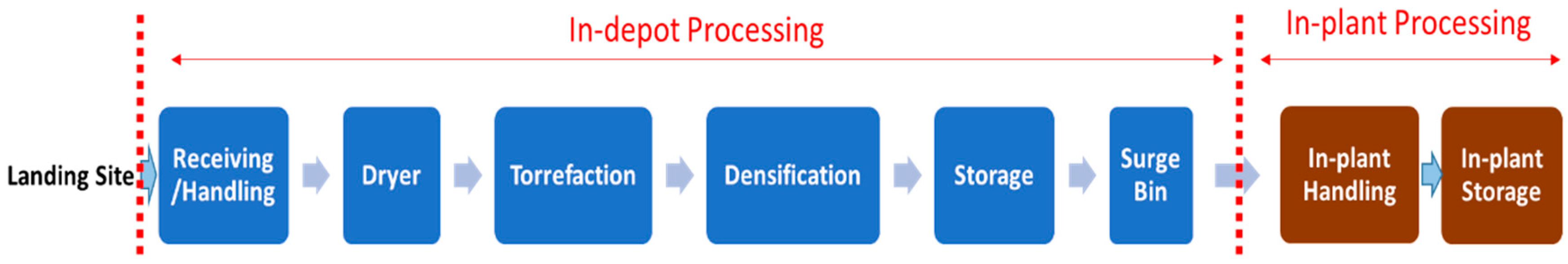
Conventional woody biomass logistics use the existing local infrastructure for feedstock resources. Wood is harvested and dried prior to collection. Dried wood is comminuted at the landing and loaded into trucks for transportation either to a trans-load terminal or directly to the power plant. When received at the power plant, the chips are cleaned, dried, and fed into the conversion process through combustion. As an alternative to the conventional system, the Idaho National Laboratory (INL) suggested advanced woody feedstock logistics [25]. A key feature of this advanced design is the integration of a local biomass-processing depot where the biomass is torrefied and densified prior to transportation to the plant, as shown in Figure 1.

In this research, terminal and depot have different characteristics: the former is a place for the collecting or trans-loading of large quantities of biomass (with no processing), while the latter includes the torrefaction processing at the site. A depot provides the opportunity to convert biomass into a consistent, stable, and flowable material early in the supply network, increasing not only conversion performance but transportation efficiency as well, whether it is by truck or rail. A depot can also include the functions of a terminal, if it is built in the existing terminal.

This paper considers both conventional and advanced logistics for determining the preferred level of co-firing. A comparative study between two feedstock logistics systems provides insights on the relationship of optimal co-firing ratio and on the type of logistics systems that would be appropriate for each coal power plant.

2.2. Seasonality

Various types of woody biomass can be turned into fuels for co-firing power plants, but this research concentrates only on forest and mill residues. Forest residues include logging residues and other removable material left after logging operations. Mill residues, on the other hand, are generated when sawlogs, pulpwood, and veneer logs are processed into conventional forest products. In this study, it is assumed that only unused mill residues (40% of total mill residues [26]) are available as a resource of biomass co-firing.

When woody biomass feedstock is used to replace some of the existing coal supply chain, the seasonal variation of each feedstock needs to be determined. It tends to be higher for forest residue than for mill residue, as supply of forest residue is directly driven by the commercial logging industry [27]. To express the supply variation of forest residue, successive time periods (t, t + 1, t + 2, …, T) are denoted in our model. More specifically, maximum quantity of forest residue usable within each time period ($t\in T$) is limited based on the shipments (in kilograms) from supplier within the corresponding time period. For mill residue, no seasonal variation is considered.

2.3. Economic Incentives and Mandates for Renewable Energy

Currently, the renewable energy industry in the US is supported through both mandates and incentives. Several states have been active in adopting or increasing Renewable Portfolio Standards (RPS) and 29 states currently mandate the utilities to sell a specified percentage or amount of renewable electricity [28]. At the federal level, incentives such as the production tax credit (PTC) support renewable energy production. The PTC is currently equal to $0.012 per kilowatt hours of electricity generated by open-loop biomass which includes any agricultural livestock waste nutrients, or any solid, nonhazardous, cellulosic waste material [29]. However, PTC for general co-firing is not clearly specified [18]. In this study, we extend PTC to support biomass co-firing with existing coal power plants in the Great Lakes States area and estimate the impacts on co-firing ratios. The benefits of potential tax credit (PTC) by biomass co-firing are set to equal the current PTC at $0.012 per kWh.

2.4. Loss of Boiler Efficiency and Maximum Co-Firing Ratio

The loss of boiler efficiency generated by woody biomass co-firing is modest [7]. In our study, a 1% drop in conversion efficiency for every 10% of mass increase in co-fired biomass is assumed [30,31]. In addition, the maximum ratio of biomass co-firing is limed to 50%, as it is known that the high ratio of biomass co-firing can significantly increase the slagging, fouling, and corrosion in the boiler [7,18]. The 50% maximum ratio for co-firing also restricts the loss of boiler efficiency to maximum 5%. To reduce the complexity of the model, we use average value of efficiency loss (2.5%) when biomass is used for co-firing. If $E^0$ is the current annual heat input of a coal power plant, the heat input $\mathrm{E}$ required to maintain the same energy output with biomass co-firing can be calculated by:

$$\mathrm{E}=(\frac{{\phi }^0}{{\phi }^0-\sigma })\times E^0$$

where ${\phi }^0$ is current boiler efficiency, and $\sigma$ is an average value of efficiency loss. This paper applies a boiler efficiency of 42% for coal [31]. Thus, if biomass is used for co-firing the heat input E required to maintain the same energy output increases to:

$$\mathrm{E}=(\frac{42\%}{42\%-2.5\%})\times E^0=(1+0.06)\times E^0$$

2.5. Mathematical Model

A mixed integer linear program (MILP) with deterministic equivalent of a stochastic problem is developed to integrate advanced woody biomass logistics with existing coal logistics system. The main purpose of our model is to determine optimal ratio of woody biomass co-firing for a coal power plant that minimizes total logistics cost and allows for considering torrefaction option. The following cost factors are accounted for in total logistics cost:

$$\begin{gathered} Total logistics cost of biomass cofiring \\ \hspace{1em}\hspace{1em}\hspace{1em}\hspace{1em}= Cos{t}^{Coal logistics}+Cos{t}^{Biomass logistics} \\ \hspace{1em}\hspace{1em}\hspace{1em}\hspace{1em}\hspace{1em}- Benefi{t}^{Tax cridit by biomass cofiring} \end{gathered}$$

The logistics cost factors consist of delivered cost of coal and woody biomass that include feedstock purchasing, transportation, and trans-loading cost in the intermediate facilities (terminals or depots). Additional capital and operation costs are accounted for at the power plant and at the intermediate facilities, when applicable.

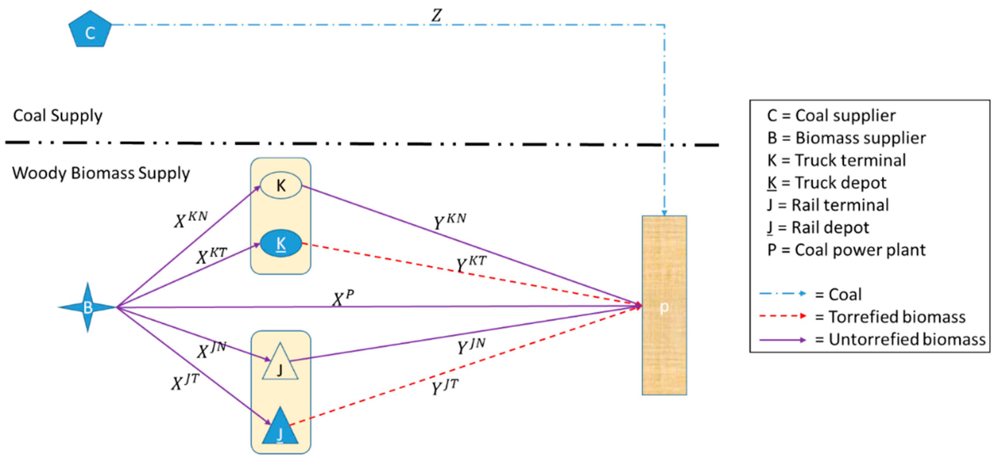
Figure 2 shows basic sets and decision variables for the mathematical model used in the research. As shown, biomass shipments for non-torrefied (N) and torrefied (T) biomass are considered separately. $X^{KN}$ and $X^{KT}$ indicate the truck flow of biomass transported from supplier (feedstock origin) to truck terminal or depot, respectively. $X^{JN}$ and $X^{JT}$ represent the truck flow of biomass transported from supplier to rail terminal or depot, respectively. $X^P$ shows the direct trucking flow of biomass transported from supplier to power plant. In addition, $Y^{KN}$ and $Y^{KT}$ indicate the truck flow of biomass transported from truck terminal and depot to power plant, respectively and for rail transportation, $Y^{JN}$ and $Y^{JT}$ show the biomass flow transported from rail terminal and depot to power plant, respectively. Please note that the two flows shipped through depots ($Y^{KT}$ and $Y^{JT}$) are torrefied woody biomass. A flow of coal from existing coal supplier to power plant is expressed by $Z$.

As mentioned earlier, the seasonal variations in feedstock yields can alter the feedstock decisions and may consequently affect the level of co-firing ratio. Hence, the impact of feedstock seasonality on logistics system is addressed by a set of successive time periods T ($t\in T)$.

All notations of sets, decision variables, and parameters used for our model are presented in

Table 1. Notation.

Set

▪ B = Set of biomass feedstock, $b\in B$

▪ I = Set of biomass feedstock supplier, $i\in I$

▪ J = Set of rail intermediate facility (terminal or depot), $j\in J$

▪ K = Set of truck intermediate facility (terminal or depot), $k\in K$

▪ T = Set of successive time periods, $t\in T$

▪ L = Set of capacity level of intermediate facility (terminal or depot), $l\in L$

Parameter

▪ $C_b^{TF}, C_b^{RF}$ = Fixed transport cost of biomass feedstock b by truck and rail, respectively ($/kg)

▪ $C_b^{TV}, C_b^{RV}$ = Variable transport cost of biomass feedstock b by truck and rail, respectively ($/kg-km)

▪ $C_b^L$ = Trans-loading cost of biomass feedstock b ($/kg)

▪ $C_b^{PU}$ = Purchasing cost of biomass feedstock b ($/kg)

▪ $f_l^{VK}, f_l^{VJ}$ = Capital cost of truck and rail terminal with capacity l, respectively ($/kg)

▪ $f_l^{WK}, f_l^{WJ}$ = Capital cost of truck and rail depot with capacity l, respectively ($/kg)

▪ $C_b^{OIN}, C_b^{OIT}$ = Operations cost in terminal and depot for biomass feedstock b, respectively ($/kg)

▪ $C_b^{CPN}, C_b^{CPT}$ = Capital cost at the plant for untorrefied and torrefied biomass b, respectively ($/kg)

▪ $C_b^{OPN}, C_b^{OPT}$ = Operation cost at the plant for untorrefied and torrefied biomass b, respectively ($/kg)

▪ $C_b^S$ = Storage cost of biomass feedstock b ($/kg)

▪ $C_t^C$ = Delivered cost of coal at period t ($/kg)

▪ $D_{ik}^{IK},D_{ij}^{IJ}$ = Distance between supplier i and truck intermediate facility j, and between supplier i and rail intermediate facility k, respectively (km)

▪ $D_i^{IP}$ = Distance between supplier i and plant (km)

▪ $D_k^{KP}, D_j^{JP}$ = Distance between truck intermediate facility k and plant, and between rail intermediate facility j and plant, respectively (km)

▪ $Q_l$ = Capacity level of intermediate facility (terminal or depot) (kg)

▪ $e_b^N, e_b^T$ = Heating value of untorrefied and torrefied biomass b, respectively (Gigajoules/kg)

▪ $e^C$ = Heating value of coal (Gigajoules/kg)

▪ $R_{ibt}$ = Maximum quantity of biomass b available from supplier i during period t (kg)

▪ $Z_t^0$ = Current demand quantity of coal shipped to plant during period t (kg)

▪ ${\theta }^V$ = Energy conversion factor from Gigajoules to kWh

▪ ${\theta }_b^M$ = Mass conversion factor of biomass feedstock b after torrefaction process (%)

▪ $\tau$ = Production tax credit ($/kWh)

▪ M = Big number

Decision Variable

▪ $X_{ibkt}^{KN}, X_{ibkt}^{KT}$ = Flow of biomass b shipped from supplier i to truck terminal k or truck depot k at period t, respectively

▪ $X_{ibjt}^{JN}, X_{ibjt}^{JT}$ = Flow of biomass b shipped from supplier i to rail terminal j or rail depot j at period t, respectively

▪ $X_{ibt}^P$ = Flow of biomass b transported directly from supplier i to plant during period t

▪ $Y_{bkt}^{KN}, Y_{bjt}^{JN}$ = Flow of untorrefied biomass b transported from truck terminal k to plant, and from rail terminal j to plant during period t, respectively

▪ $Y_{bkt}^{KT}$, $Y_{bjt}^{JT}$ = Flow of torrefied biomass b transported from truck depot k to plant, and from rail depot j to plant during period t, respectively

▪ $V_{klt}^K$ = 1 if truck terminal k with capacity level l is used during period t, 0 otherwise

▪ $W_{klt}^K$ = 1 if truck depot with capacity level l is built at truck terminal k during period t, 0 otherwise

▪ $V_{jlt}^J$ = 1 if rail terminal j with capacity level l is used during period t, 0 otherwise

▪ $W_{jlt}^J$ = 1 if rail depot with capacity level l is built at rail terminal j during period t, 0 otherwise

▪ $S_{bkt}^{KN}, S_{bjt}^{JN}$ = Untorrefied biomass b stored at truck terminal k, and at rail terminal j during period t, respectively

▪ $S_{bkt}^{KT}$, $S_{bjt}^{JT}$ = Torrefied biomass b stored at truck terminal k, and at rail terminal j during period t, respectively

▪ $Z_t$ = Flow of coal shipped to plant during period t

▪ ${\alpha }_t, {\beta }_t$ = Random variable

▪ ${\gamma }_t$= Binary variable

and described in the following section.

The mathematical formulation of our MILP problem is provided below. Expressions (1) to (9) indicate the terms of objective function, and expressions (10) to (34) demonstrate the constraints of the model.

$$Min {\displaystyle \sum }_l{\displaystyle \sum }_t\left[{\displaystyle \sum }_k(f_l^{VK}·V_{klt}^K+f_l^{WK}·W_{klt}^K)+{\displaystyle \sum }_j(f_l^{VJ}·V_{jlt}^J+f_l^{WJ}·W_{jlt}^J)\right]$$

(1)

$$\begin{gathered} +{\displaystyle \sum }_b{\displaystyle \sum }_t[{\displaystyle \sum }_i{\displaystyle \sum }_k(C_b^{TF}+C_b^{TV}·D_{ik}^{IK})(X_{ibkt}^{KN}+X_{ibkt}^{KT}) \\ \hspace{1em}\hspace{1em}\hspace{1em}+{\displaystyle \sum }_i{\displaystyle \sum }_j(C_b^{TF}+C_b^{TV}·D_{ij}^{IJ})(X_{ibjt}^{JN}+X_{ibjt}^{JT}) \\ \hspace{1em}\hspace{1em}\hspace{1em}\hspace{1em}\hspace{1em}+{\displaystyle \sum }_k(C_b^{TF}+C_b^{TV}·D_k^{KP}+C_b^L)(Y_{bkt}^{KN}+Y_{bkt}^{KT}) \\ \hspace{1em}\hspace{1em}\hspace{1em}\hspace{1em}+{\displaystyle \sum }_j^k(C_b^{RF}+C_b^{RV}·D_j^{JP}+C_b^L)(Y_{bjt}^{JN}+Y_{bjt}^{JT}) \\ \hspace{1em}\hspace{1em}+{\displaystyle \sum }_i(C_b^{TF}+C_b^{TV}·D_i^{IP})X_{ibt}^P \end{gathered}$$

(2)

$$+{\displaystyle \sum }_i{\displaystyle \sum }_b{\displaystyle \sum }_t{\displaystyle \sum }_k{\displaystyle \sum }_j{C}_b^{PU}(X_{ibkt}^{KN}+X_{ibkt}^{KT}+X_{ibjt}^{JN}+X_{ibjt}^{JT}+X_{ibt}^P)$$

(3)

$$+{\displaystyle \sum }_i{\displaystyle \sum }_b{\displaystyle \sum }_t{\displaystyle \sum }_k{\displaystyle \sum }_j\left\{C_b^{OIN}(X_{ibkt}^{KN}+X_{ibjt}^{JN})+C_b^{OIT}(X_{ibkt}^{KT}+X_{ibjt}^{JT})\right\}$$

(4)

$$+{\displaystyle \sum }_b{\displaystyle \sum }_t{\displaystyle \sum }_k{\displaystyle \sum }_j\left\{C_b^{CPN}(Y_{bkt}^{KN}+Y_{bjt}^{JN}+X_{ibt}^P)+C_b^{CPT}(Y_{bkt}^{KT}+Y_{bjt}^{JT})\right\}$$

(5)

$$+{\displaystyle \sum }_b{\displaystyle \sum }_t{\displaystyle \sum }_k{\displaystyle \sum }_j\left\{C_b^{OPN}(Y_{bkt}^{KN}+Y_{bjt}^{JN}+X_{ibt}^P)+C_b^{OPT}(Y_{bkt}^{KT}+Y_{bjt}^{JT})\right\}$$

(6)

$$+{\displaystyle \sum }_b{\displaystyle \sum }_t{\displaystyle \sum }_k{\displaystyle \sum }_j{C}_b^S\left\{(S_{bkt}^{KN}+S_{bjt}^{JN})+(S_{bkt}^{KT}+S_{bjt}^{JT})\right\}$$

(7)

$$+{\displaystyle \sum }_t{C}_t^C·Z_t$$

(8)

$$-{\displaystyle \sum }_b{\displaystyle \sum }_t{\displaystyle \sum }_k{\displaystyle \sum }_j\tau \left\{\frac{e_b^N}{{\theta }^V}(Y_{bkt}^{KN}+Y_{bjt}^{JN}+X_{ibt}^P)+\frac{e_b^T}{{\theta }^V}(Y_{bkt}^{KT}+Y_{bjt}^{JT})\right\}$$

(9)

s.t.

$${\displaystyle \sum }_t{\displaystyle \sum }_i{\displaystyle \sum }_b{X}_{ibkt}^{KN}\le {\displaystyle \sum }_l{\displaystyle \sum }_t{Q}_l(V_{klt}^K-W_{klt}^K) \forall k\in K$$

(10)

$${\displaystyle \sum }_t{\displaystyle \sum }_i{\displaystyle \sum }_b{X}_{ibjt}^{JN}\le {\displaystyle \sum }_l{\displaystyle \sum }_t{Q}_l(V_{jlt}^J-W_{jlt}^J) \forall j\in J$$

(11)

$${\displaystyle \sum }_t{\displaystyle \sum }_i{\displaystyle \sum }_b{X}_{ibkt}^{KT}\le {\displaystyle \sum }_l{\displaystyle \sum }_t{Q}_l·W_{klt}^K \forall k\in K$$

(12)

$${\displaystyle \sum }_t{\displaystyle \sum }_i{\displaystyle \sum }_b{X}_{ibjt}^{JT}\le {\displaystyle \sum }_l{\displaystyle \sum }_t{Q}_l·W_{jlt}^J \forall j\in J$$

(13)

$${\displaystyle \sum }_i{X}_{ibkt}^{KN}=Y_{bkt}^{KN}+S_{bkt}^{KN}-S_{bk(t-1)}^{KN} \forall k\in K,b\in B, t\in T$$

(14)

$${\theta }_b^M·{\displaystyle \sum }_i{X}_{ibkt}^{KT}=Y_{bkt}^{KT}+S_{bkt}^{KT}-S_{bk(t-1)}^{KT} \forall k\in K,b\in B,t\in T$$

(15)

$${\displaystyle \sum }_i{X}_{ibjt}^{JN}=Y_{bjt}^{JN}+S_{bjt}^{JN}-S_{bj(t-1)}^{JN} \forall j\in J,b\in B, t\in T$$

(16)

$${\theta }_b^M·{\displaystyle \sum }_i{X}_{ibjt}^{JT}=Y_{bjt}^{JT}+S_{bjt}^{JT}-S_{bj(t-1)}^{JT} \forall j\in J,b\in B,t\in T$$

(17)

$$W_{klt}^K\le V_{klt}^K \forall k\in K, l\in L,t\in T$$

(18)

$$W_{jlt}^J\le V_{jlt}^J \forall j\in J, l\in L,t\in T$$

(19)

$${\displaystyle \sum }_l{\displaystyle \sum }_t{V}_{klt}^K\le 1 \forall k\in K$$

(20)

$${\displaystyle \sum }_l{\displaystyle \sum }_t{V}_{jlt}^J\le 1 \forall j\in J$$

(21)

$${\displaystyle \sum }_t{\displaystyle \sum }_b{S}_{bkt}^{KN}\le {\displaystyle \sum }_l{\displaystyle \sum }_t{Q}_l(V_{klt}^K-W_{klt}^K) \forall k\in K$$

(22)

$${\displaystyle \sum }_t{\displaystyle \sum }_b{S}_{bjt}^{JN}\le {\displaystyle \sum }_l{\displaystyle \sum }_t{Q}_l(V_{jlt}^J-W_{jlt}^J) \forall j\in J$$

(23)

$${\displaystyle \sum }_t{\displaystyle \sum }_b{S}_{bkt}^{KT}\le {\displaystyle \sum }_l{\displaystyle \sum }_t{Q}_l·W_{klt}^K \forall k\in K$$

(24)

$${\displaystyle \sum }_t{\displaystyle \sum }_b{S}_{bjt}^{JT}\le {\displaystyle \sum }_l{\displaystyle \sum }_t{Q}_l·W_{jlt}^J \forall j\in J$$

(25)

$${\displaystyle \sum }_k{\displaystyle \sum }_j{\displaystyle \sum }_t(X_{ibkt}^{KN}+X_{ibkt}^{KT}+X_{ibjt}^{JN}+X_{ibjt}^{JT}+X_{ibt}^P)\le R_{ibt} \forall i\in I,b\in B, \forall t\in T$$

(26)

$$\left\{\frac{{{\displaystyle \sum }}_k{{\displaystyle \sum }}_j{{\displaystyle \sum }}_b(Y_{bkt}^{KN}+Y_{bjt}^{JN}+X_{ibt}^P+Y_{bkt}^{KT}+Y_{bjt}^{JT})}{{{\displaystyle \sum }}_k{{\displaystyle \sum }}_j{{\displaystyle \sum }}_b(Y_{bkt}^{KN}+Y_{bjt}^{JN}+X_{ibt}^P+Y_{bkt}^{KT}+Y_{bjt}^{JT})+Z_t}\right\}\le 0.5 t\in T$$

(27)

$${\displaystyle \sum }_k{\displaystyle \sum }_j{\displaystyle \sum }_b\left\{e_b^N(Y_{bkt}^{KN}+Y_{bjt}^{JN}+X_{ibt}^P)+e_b^T(Y_{bkt}^{KT}+Y_{bjt}^{JT})\right\}+e^C·Z_t\ge (1+{\alpha }_t)·e^C·Z_t^O \forall t\in T$$

(28)

$${\displaystyle \sum }_k{\displaystyle \sum }_j{\displaystyle \sum }_b(Y_{bkt}^{KN}+Y_{bjt}^{JN}+X_{ibt}^P+Y_{bkt}^{KT}+Y_{bjt}^{JT})\ge {\gamma }_t \forall t\in T$$

(29)

$${\gamma }_t\ge \frac{1}{M}{\displaystyle \sum }_k{\displaystyle \sum }_j{\displaystyle \sum }_b(Y_{bkt}^{KN}+Y_{bjt}^{JN}+X_{ibt}^P+Y_{bkt}^{KT}+Y_{bjt}^{JT}) \forall t\in T$$

(30)

$${\alpha }_t\le M·{\gamma }_t \forall t\in T$$

(31)

$${\beta }_t\le M(1-{\gamma }_t) \forall t\in T$$

(32)

$${\alpha }_t=0.06-{\beta }_t \forall t\in T$$

(33)

$$V_{klt}^K,W_{klt}^K, V_{jlt}^J, W_{jlt}^J,{\gamma }_t \in \left\{0,1\right\}, All other decision variables \ge 0$$

(34)

The first term (1) of objective function of this optimization model indicates the capital costs for new intermediate facility (terminal or depot) using either truck or rail. Each terminal and depot has maximum annual capacity limit of biomass processing (in kilograms). The second term (2) of the objective function indicates the sum of shipping costs for single- and multi-modal transportation between supply areas, intermediate facilities, and a power plant. Transportation cost is divided into a distance-fixed cost and the distance-variable cost. Please note that a trans-loading cost is accounted for at terminals and depots. The third term (3) of the objective function expresses the purchasing cost of each type of biomass feedstock. The fourth term (4) describes the operations costs in terminal and depot for biomass feedstock. Different operation costs are applied to terminal and depot, as torrefaction can occur in depot only. The fifth term (5) represents capital costs for in-plant processing such as handling, drying and storage at the power plant. Please note that untorrefied and torrefied biomass require different in-plant processing. The term (6) of objective function indicates operations costs at the power plant applied to untorrefied and torrefied biomass separately. The seventh term (7) expresses the storage costs in biomass terminal or depot. The eighth term (8) indicates the delivered costs of coal. In this paper, we use parameters from an existing coal supply chain system and assume that co-firing does not affect the coal delivery factors, such as rates and coal transportation mode. The final term (9) of the objective function presents the potential economic benefits that could be obtained from PTC for the use of biomass feedstock.

Constraints (10)–(13) ensure that biomass is transported to intermediate facility only if it is open. At the same time, they define the annual capacity limitations of the facility and ensure that all biomass feedstocks shipped to a depot are upgraded by torrefaction process. Constraints (14)–(17) are flow balance constraints for intermediate facilities, which ensure the equality of incoming and outgoing biomass flows at corresponding facilities. Since this model accounts for the seasonal variation within each time period (e.g., month), biomass stored in previous time period t−1 can be used during the next time period t. As torrefaction contributes to the mass reduction, a typical mass conversion factor is considered for torrefied biomass in constraints (15) and (17). Constraints (18)–(19) ensure that a depot is built only in the terminal is determined to be used. Constraints (20)–(21) make sure that no more than one facility (for terminal and depot, respectively) can open at a given location. Constraint (22)–(25) ensure that biomass is stored at intermediate facility only if it is open while, at the same time, dictating the maximum annual storage capacity for the facility. In our study, three annual capacity levels ($Q_l$) of terminal/depot were assumed; 45, 91 and 136 million kilograms (50, 100 and 150 thousand tons) per year. Constraint (26) ensures that biomass outflow from a supply area during a time period is less than its supply availability in a corresponding period. Constraint (27) expresses the maximum level of biomass co-firing calculated by mass of biomass co-fired over total mass of feedstock used at the power plant. Please note that maximum biomass co-firing ratio is restricted to 50% of the total mass.

Demand satisfaction in terms of energy value is addressed in constraint (28) which is followed by constraints (29)–(33) that indicate the “Either-Or” constraints to consider the loss of boiler efficiency from biomass co-firing. The two positive random variables (${\alpha }_t, {\beta }_t$) and a binary variable (${\gamma }_t$) are used to build the Either-Or constraint set. This constraint set ensures the heat input required to maintain the same energy output increases, if co-firing is used. Finally, constraint (34) defines binary and non-negativity requirements for the decision variables.

To estimate the impact of advanced logistics system, this study also considers conventional logistics system. The mathematical model for conventional logistics system is developed simply by removing the feedstock upgrading options from advanced logistics model. Thus, the level of biomass co-firing in “conventional logistics only” scenario can be calculated by limiting the values of all decision variables related to building depots to “zero” (i.e., ${{\displaystyle \sum }}_k{{\displaystyle \sum }}_l{{\displaystyle \sum }}_t{W}_{klt}^K={{\displaystyle \sum }}_j{{\displaystyle \sum }}_l{{\displaystyle \sum }}_t{W}_{jlt}^J=0$).

2.6. The Solution Approaches

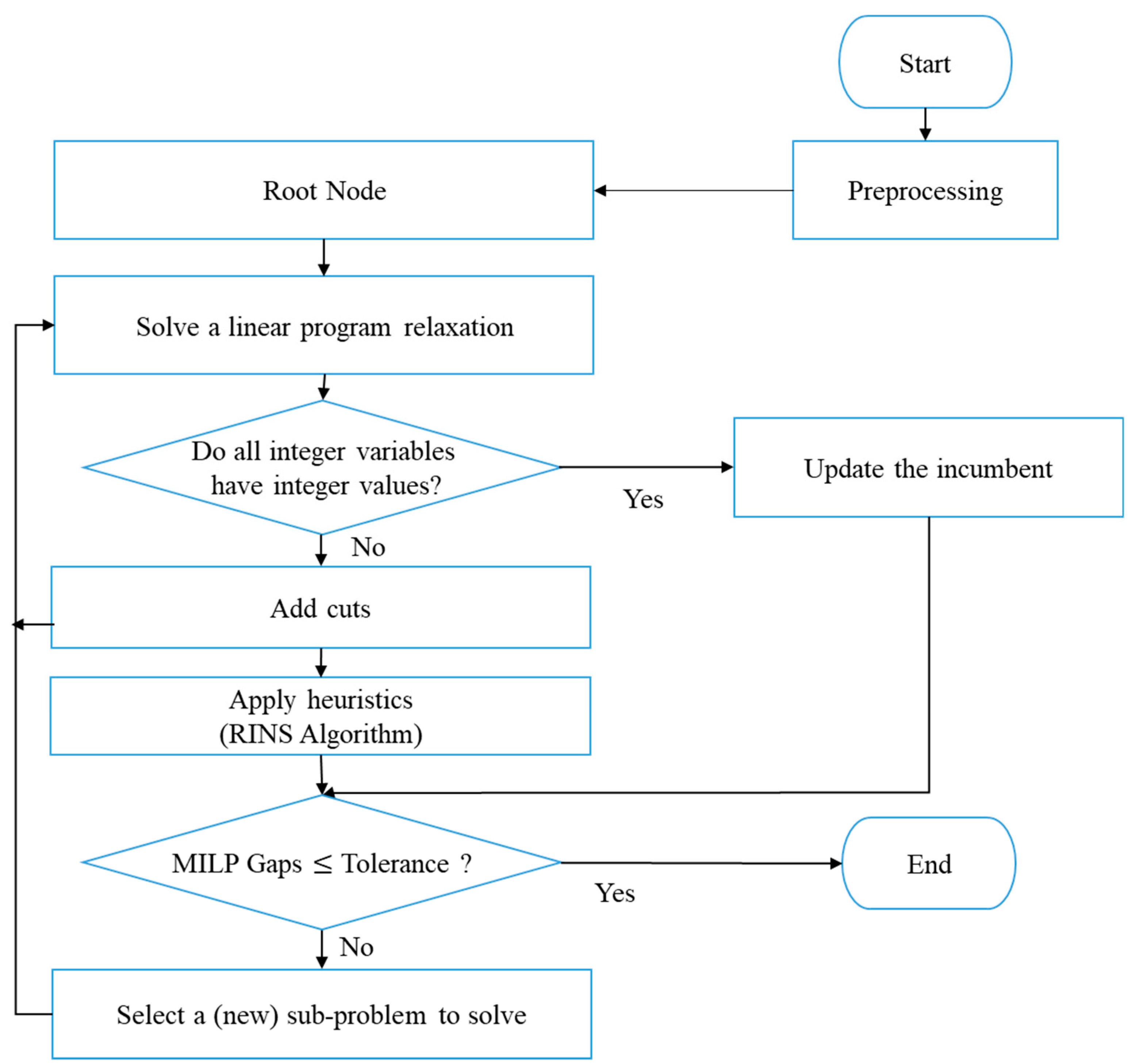
In this study, we use the MILP solver of IBM ILOG CPLEX Optimization Studio 12.7 with Python API (Application Programming Interfaces), which is based on the dynamic search algorithm. The dynamic search algorithm in CPLEX basically consists of four blocks to solve large scale MILP problem: pre-processing, LP relaxation, branch and cuts, and heuristics [32]. Pre-processing step reduces the size of the problem and improves the formulation through a probing technique that analyses the logical implications of fixing each binary variable to 0 or 1. For heuristics, the relaxation induced neighborhood search (RINS) algorithm is selected in this study. RINS algorithm is based on the fact that the solution of the continuous relaxation at the current node is most often not integral, but its objective value is always better than that of the incumbent [33]. RINS sets an objective cut-off based on the variables that have the same values in the incumbent and in the current continuous relaxation, and then solves a sub-MILP on the remaining variables. The flow chart in Figure 3 shows the steps of solving process in CPLEX. The details of this built-in CPLEX algorithm is shown in an IBM document [34]. All experiments were run on a 3.6 GHz Core i7 processor with 16 Gbytes of RAM (Random Access Memory).

3. Results and Discussions: Case Study of Optimal Level of Woody Biomass for Co-Firing in Existing Coal Power Plants in the Great Lakes States of the US

3.1. Data Collection and Pre-Processing

This section describes the case study used to test the model. It estimates the optimal level of woody biomass co-firing and related logistics for existing 26 coal power plants in three Great Lakes States; Michigan (MI), Wisconsin (WI), and Minnesota (MN). In this research, our model is applied to each power plant independently, as it addresses a user optimization rather than public/system optimization.

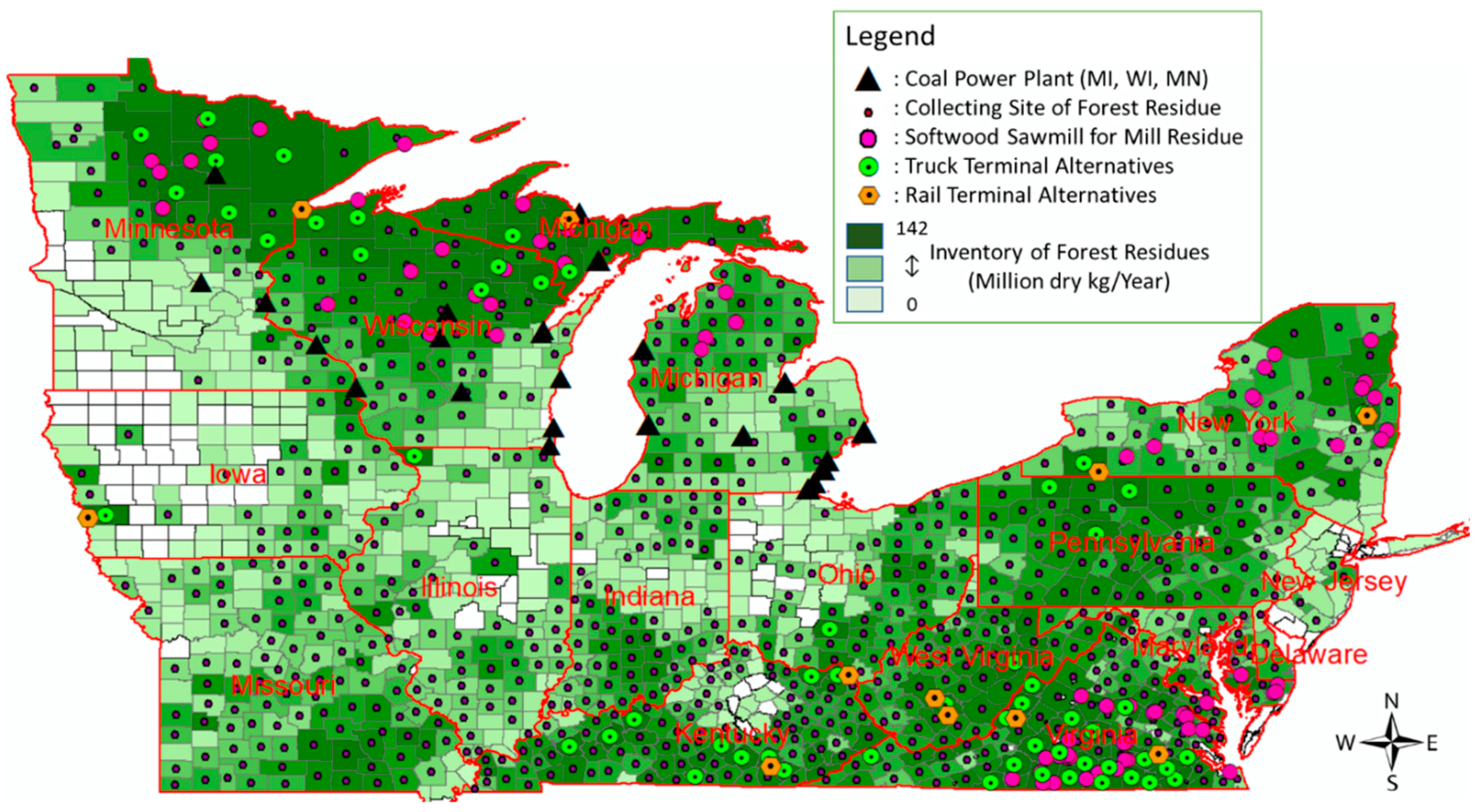
Majority of data collection and pre-processing is based on Ko and Lautala [36] which also includes a detailed description of pre-processing steps. The procurement areas for woody biomass feedstock cover softwood sawmills (for mill residues) and collection points (for forest residues) located in the centroid of each county within the 16 states that cover all potential feedstock origins (Figure 4). The available locations of biomass supply consist of 845 counties for forest residues and 74 softwood sawmills. For transportation facilities, 58 truck and 11 rail locations are identified as potential terminal/depot sites for the case study. All spatial analysis, such as distances between origin-destination (O/D) pairs, are determined in the Network Analyst of ArcGIS 10.5 based on actual road and rail network provided by the US Department of Transportation [37]. Values for the following parameters are taken from Ko and Lautala [36], and provided at

Table A1. Input data for woody biomass feedstock (Ko and Lautala [36]).

Data		Value	Reference
Feedstock Availability	Forest Residue	Kilograms for 845 potential collecting sites in 16 States	US Department of Agriculture (USDA) [40]
	Mill Residue	Kilograms for 74 Softwood Sawmills in 16 States	USDA Forest Service [41]
Feedstock Purchasing Cost	Forest Residue	$0.017/kg	US Department of Energy [26]
	Mill Residue	$0.024/kg
Transport Rate	Truck Rate ($/Thousand kg) $x=distance between O-D$	Before Terminal: $0.0939x+5.8494$ After Terminal: $0.0642x+7.8778$	Interview with Local Forest Company [36]
	Rail Rate ($/Carload) $x=distance between O-D$	CN Rail: $4.8698x+1512$ NS Rail: $4.1774x+2136$	Official Tariffs [42,43]; Interview with Local Forest Company [36]
Energy Contents (Before & After torrefaction)	Forest Residue	0.011 GJ/kg & 0.015 GJ/kg	US EPA [44]; Van der Stelt et al. [11]
	Mill Residue	0.019 GJ/kg & 0.025 GJ/kg
	Coal	0.029 GJ/kg
Mass conversion factor after torrefaction (${\theta }_b^M)$		1.43	Dutta and Leon [12]
Storage Cost of Biomass Feedstock ($C_b^S)$		$0.639/Thousand kg	Zhang et al. [45]

and

Table A2. Capital and operation costs of conventional and advanced logistics for woody biomass co-firing (Ko and Lautala [36]).

Capital Cost/Operation Cost (2016 US $ Per Dry Thousand kg)		Processes in Terminal or Depot							Processes in Power Plant
		Receiving/Handling	Dryer	Torre-Faction	Densifi-Cation	Storage	Surge Bin	Sum	In-Plant Handling	In-Plant Drying	In-Plant Storage	Sum
Conventional Logistics	(1) Supply area ↓ Power Plant	n/a	n/a	n/a	n/a	n/a	n/a	0.0/0.0	19.75/4.72	39.14/12.68	3.63/1.17	62.52/18.56
	(2) Supply area ↓ Terminal ↓ Power Plant	12.04/2.71	n/a	n/a	n/a	3.59/1.14	0.86/0.08	16.49/3.92	19.75/4.72	39.14/12.68	3.63/1.17	62.52/18.56
Advanced Logistics	(3) Supply area ↓ Terminal + Depot ↓ Power Plant	12.04/2.71	45.83/17.34	75.73/11.18	3.16/6.16	3.59/1.14	0.86/0.08	141.2/38.6	0.67/0.2	n/a	3.63/1.17	4.3/1.37

Source: Adapted from Boardman et al. [25].

in Appendix A.

-

Feedstock availability

-

Alternative locations for truck and rail terminals

-

Purchase cost of woody biomass feedstock

-

Transportation cost for truck and rail

-

Capital and operation cost occurred at both terminal/depot and power plant locations

3.1.1. Data for Coal Power Plants

The US Energy Information Administration (EIA) provides the nameplate capacities, annual coal kilograms shipped and heat input rates for all coal power plants in the US. We focus on 26 coal power plants operated in the three Great Lakes States using the 2016 EIA-923 database [38]. We use the delivered cost of coal shipped by month to each coal power plant, provided in the same database. The total cost covers all cost components incurred in the purchase and delivery of the fuel to the plant, including maintenance and depreciation costs of coal delivered in railcars owned by the plant [39].

Table 2. Names, states, delivered costs, and input energy required by coal power plants (2016).

Number	Plant Name	State	Average Delivered Costs of Coal ($/kg)	Average Input Energy Required by Month (MMBTU)
1	Presque Isle	MI	0.249	2,125,153
2	Escanaba Mill	MI	0.249	25,315
3	J H Campbell	MI	0.266	5,533,214
4	J C Weadock	MI	0.267	253,890
5	J R Whiting	MI	0.244	211,879
6	Monroe (MI)	MI	0.254	10,732,869
7	River Rouge	MI	0.246	434,755
8	St Clair	MI	0.270	418,851
9	Trenton Channel	MI	0.259	1,567,210
10	Eckert Station	MI	0.267	595,575
11	BRSC Shared Storage	MI	0.223	8,571,533
12	TES Filer City Station	MI	0.239	466,748
13	Clay Boswell	MN	0.220	5,907,394
14	Allen S King	MN	0.236	2,103,891
15	South Oak Creek	WI	0.216	3,228,271
16	Edgewater	WI	0.249	2,752,947
17	Pulliam	WI	0.269	177,931
18	Weston	WI	0.257	2,941,119
19	Genoa	WI	0.293	1,242,263
20	John P Madgett	WI	0.251	1,714,462
21	Sherburne County	MN	0.228	10,074,508
22	Pleasant Prairie	WI	0.195	5,668,994
23	Columbia (WI)	WI	0.271	3,923,054
24	Biron Mill	WI	0.257	284,699
25	Green Bay West Mill	WI	0.269	151,019
26	Elm Road Generating Station	WI	0.265	5,920,150

Source: Adapted from 2016 EIA-923 [38].

shows the names, locations (states), coal delivered costs, and input energy demanded by all 26 coal power plants used in the study.

3.1.2. Data for Seasonal Variations of Feedstocks

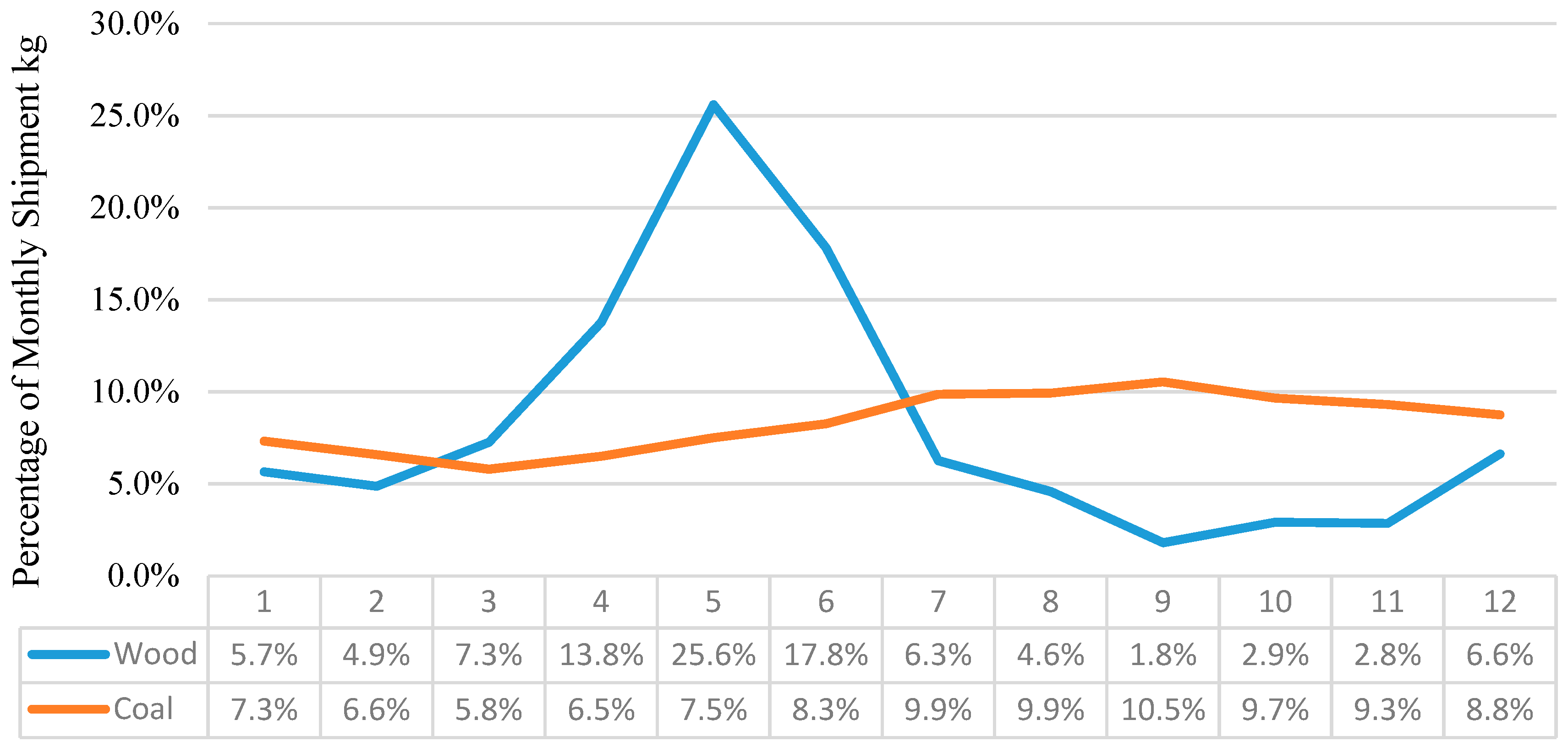
We compare the actual monthly variations of supply shipments for wood and coal (Figure 5). The monthly breakdown of woody biomass and coal shipments within each time period is also given in the bottom of the figure. The seasonal variation in wood shipment data is estimated based on actual flow data from three log satellite yards in the Great Lakes States region. We assumed that maximum quantity of forest residue usable within each time period ($t\in T$) is limited to the monthly percentage of forest residue shipments in that time period. The coal supply data is based on 26 existing coal power plants located in the same region [38].

3.2. Experimental Results

The mathematical model is applied in four different scenarios. We estimate the impacts of torrefaction option in logistics system with/without potential tax credit (PTC) to support biomass co-firing with existing coal power plants. Thus, four scenarios are developed, based on the biomass logistics system used and the availability of tax credit. The scenarios include:

-

Scenario 1: Conventional logistics with no tax credit

-

Scenario 2: Conventional logistics with tax credit

-

Scenario 3: Advanced logistics with no tax credit

-

Scenario 4: Advanced logistics with tax credit

3.2.1. Biomass Co-Firing Ratio and Cost Savings

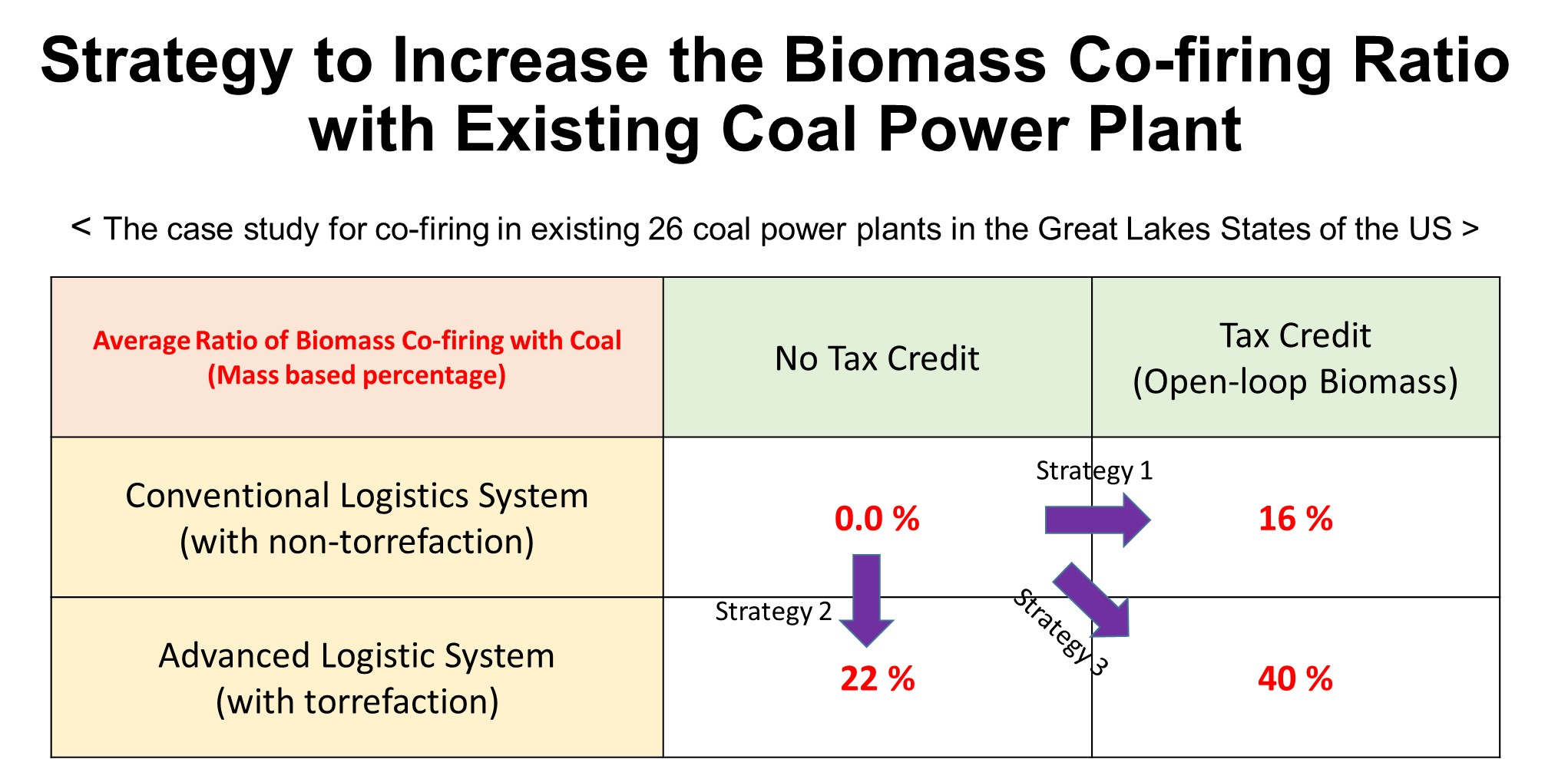
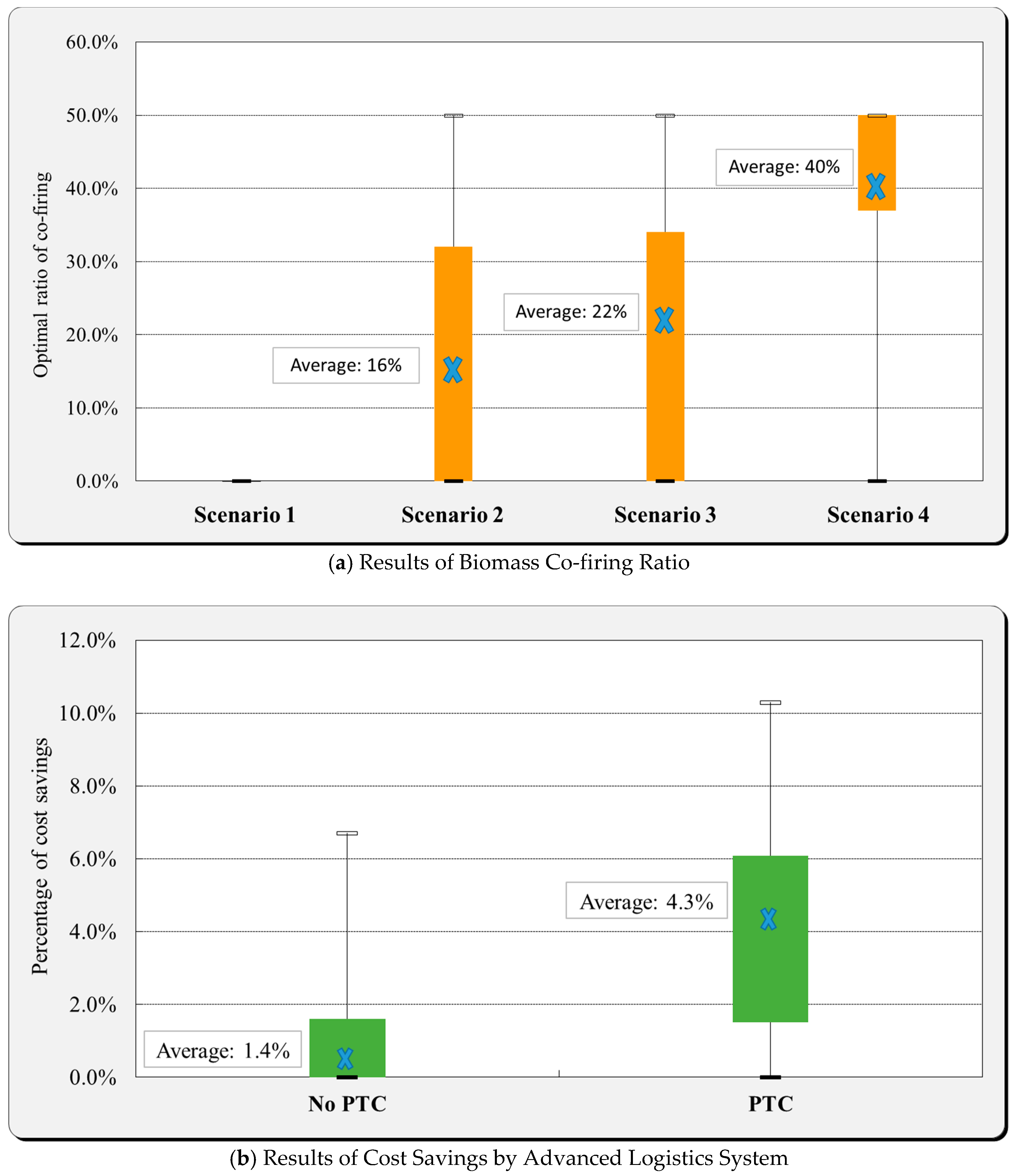
Figure 6a presents the model’s suggested level of biomass co-firing at each coal power plant, divided by scenario type. The figure shows both the average value and the 25 and 75 percentile. In the current scenario (Scenario 1), all power plants are relying fully on coal-fired power generation. There are large differences in the level of co-firing among individual plants for the other three scenarios and the average percentage of co-firing keeps increasing to 16, 22, and 40 percent, as we move to scenarios 2, 3, and 4, respectively. The variation between plants is especially high in Scenarios 2 and 3. The fact that average percentage of co-firing ratio in Scenario 3 is higher than one in scenario 2 indicates that torrefaction has higher impact on increasing the level of co-firing than the potential tax credit.

Figure 6b presents the cost savings from advanced logistics system calculated by cost difference between conventional and advanced system for each power plant. Similar to co-firing ratio, the level of savings varies greatly between individual plants. On average, the cost savings for advanced logistics without tax credit are fairly small (1.4%), as most savings are cancelled out by necessary investments in the components of the advanced logistics system. In other words, cost savings from decreased truck transportation are offset by increased rail shipments and loading costs. Likewise, savings from in-plant capital and operational costs are cancelled out by increased capital and operation costs at the depots where torrefaction takes place. If tax credits are made available, the average of cost savings increase from 1.4% to 4.3%. In one individual plant, they even reach double digits. Detail results for all power plants are provided at

Table A3. Individual plant results of biomass co-firing ratios and cost savings by advanced logistics system.

	Level of Biomass Co-Firing (Mass Base)				Cost Savings by Changing Logistics System $(=\frac{\mathit{C}\mathit{o}\mathit{s}\mathit{t} \mathit{o}\mathit{f} \mathit{C}\mathit{L}-\mathit{C}\mathit{o}\mathit{s}\mathit{t} \mathit{o}\mathit{f}\mathit{A}\mathit{L}}{\mathit{C}\mathit{o}\mathit{s}\mathit{t} \mathit{o}\mathit{f} \mathit{C}\mathit{L}})$
	Scenario 1 CL + No PTC	Scenario 2 CL + PTC	Scenario 3 AL + No PTC	Scenario 4 AL + PTC	No PTC	PTC
Plant 1	0%	16%	27%	50%	1.5%	5.6%
Plant 2	0%	50%	0%	50%	0.0%	0.0%
Plant 3	0%	0%	14%	35%	0.4%	2.7%
Plant 4	0%	47%	50%	50%	4.6%	8.1%
Plant 5	0%	0%	0%	50%	0.0%	4.7%
Plant 6	0%	0%	0%	19%	0.0%	1.1%
Plant 7	0%	16%	31%	50%	0.1%	4.6%
Plant 8	0%	33%	35%	50%	2.6%	6.7%
Plant 9	0%	0%	27%	50%	0.7%	6.5%
Plant 10	0%	29%	46%	50%	2.9%	8.0%
Plant 11	0%	0%	0%	5%	0.0%	0.0%
Plant 12	0%	16%	31%	50%	0.5%	4.8%
Plant 13	0%	0%	0%	14%	0.0%	0.7%
Plant 14	0%	0%	14%	43%	0.2%	3.5%
Plant 15	0%	0%	0%	18%	0.0%	0.9%
Plant 16	0%	0%	16%	50%	0.6%	4.6%
Plant 17	0%	50%	50%	50%	3.9%	5.9%
Plant 18	0%	6%	18%	50%	1.2%	5.6%
Plant 19	0%	47%	50%	50%	6.7%	10.3%
Plant 20	0%	6%	25%	46%	1.4%	6.1%
Plant 21	0%	0%	0%	9%	0.0%	0.4%
Plant 22	0%	0%	0%	0%	0.0%	0.0%
Plant 23	0%	6%	31%	50%	1.6%	6.0%
Plant 24	0%	47%	50%	50%	5.5%	9.5%
Plant 25	0%	50%	50%	50%	1.6%	3.3%
Plant 26	0%	0%	17%	47%	0.6%	3.3%
Average, %	0%	16%	22%	40%	1.4%	4.3%

CL: Conventional Logistics System; AL: Advanced Logistics System.

in Appendix B.

3.2.2. Biomass Feedstock Types and Transportation Mode

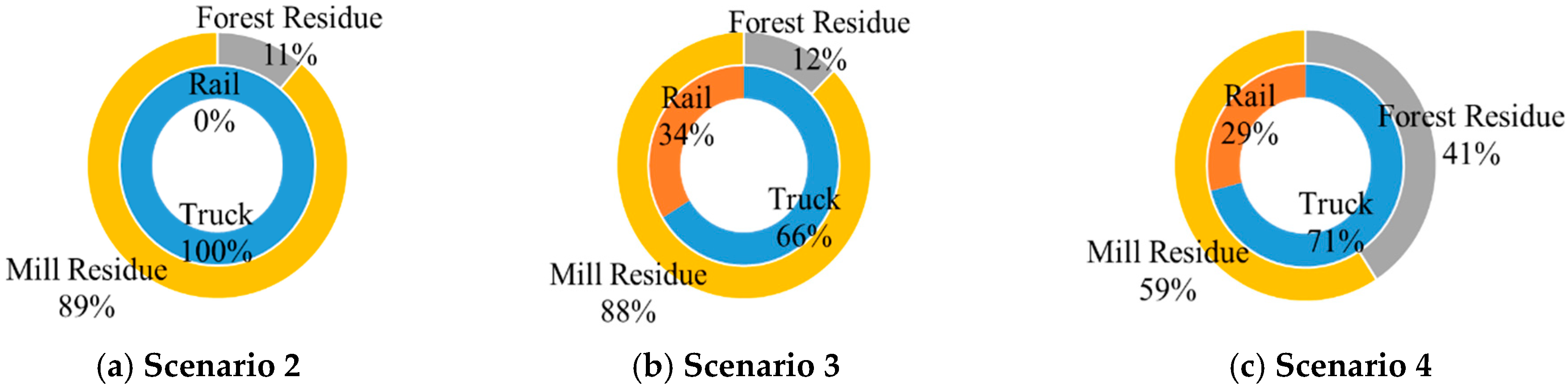
The total amount of biomass (in kilograms) used for co-firing in each scenario by all 26 coal power plants is presented in Figure 7. The use of biomass increases to 1.2, 3.4, and 19.6 billion kilograms in scenarios 2, 3 and 4, respectively. Since no coal power plants used biomass co-firing in scenario 1, it has been excluded in the figure.

Figure 7 also illustrates the breakdown of feedstock and transportation modes used in each scenario. The figure reveals that mill residue is the preferred feedstock in all scenarios, mainly due to its higher energy density. As the need for biomass feedstock increases, so does the portion of forest residues, mainly due to limited availability of mill residues. Truck is the dominant transportation mode for all co-firing scenarios, but both scenarios that use advanced logistics (3 and 4) also use noticeable amounts of rail shipments.

3.2.3. Relationship between Logistics Conditions and Co-Firing Ratio

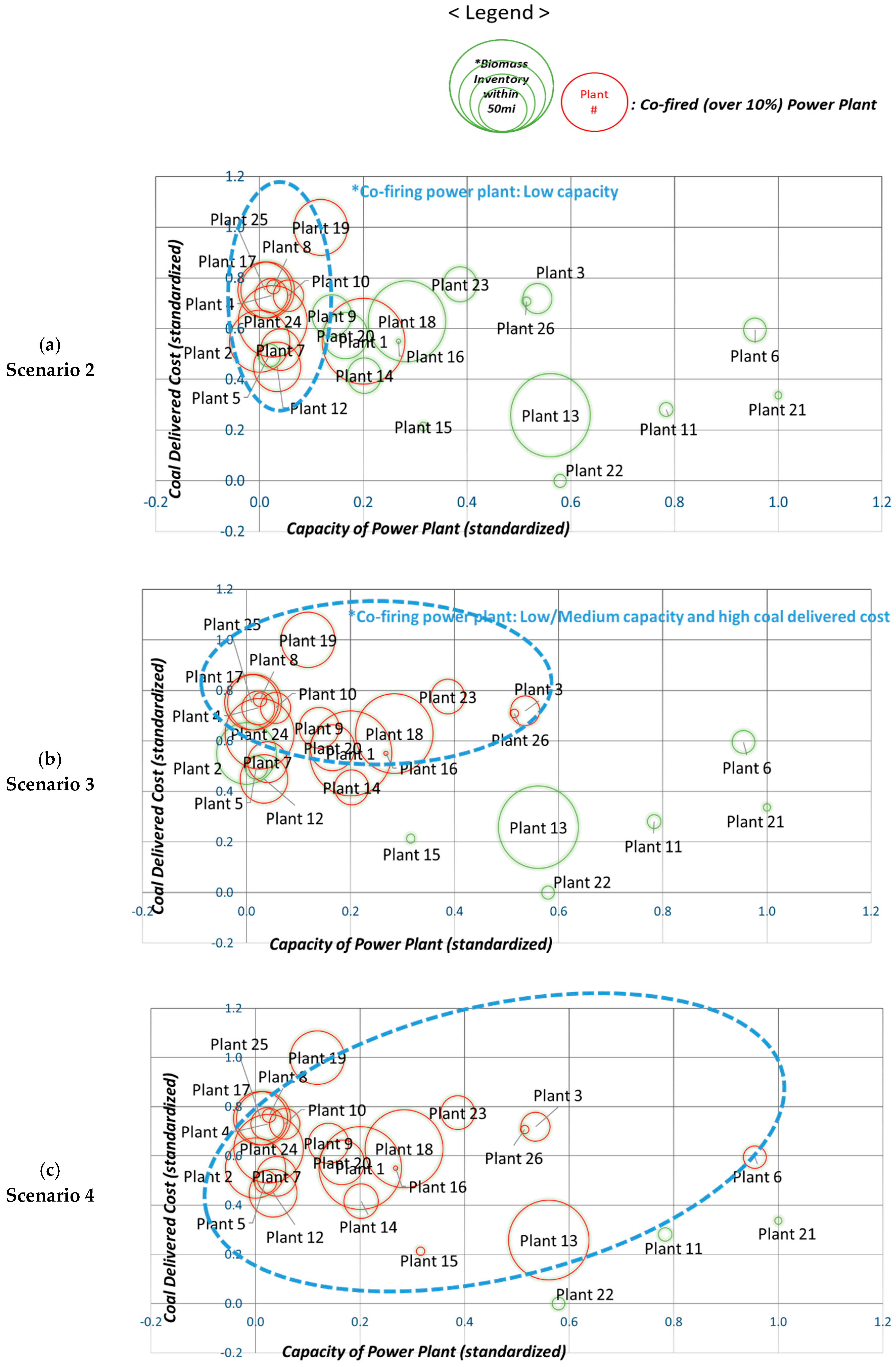
This section investigates the parameters that cause the variation in co-firing between different power plants. Three key parameters are used in the analysis; (1) capacity of coal power plant; (2) current delivered cost of coal; and (3) biomass inventory within 80 km (50 miles) from power plant. These parameters are standardized (between 0 and 1) to avoid concentration on parameter with a larger variance. Figure 8 shows the experimental results between these key parameters and co-firing ratio by scenario. The green circle indicates the level biomass inventory in the vicinity of power plant. Increasing size of a green circle indicates higher availability of nearby biomass. Red circle shows the power plants that use over 10% biomass co-firing.

Scenario 1 is excluded from the analysis, as no co-firing is used by the plants. Figure 8a demonstrates co-firing in scenario 2 (conventional logistics system with tax credit). The figure reveals that the plants using over 10% of co-firing are mainly those with low capacity. This indicates that tax credit with conventional logistics system would facilitate the use of biomass, but the effect would be limited to the smaller power plants. For the case of advanced logistics system with no tax credit (Figure 8b), co-firing is extended to the power plants that have medium level of capacity. However, power plants with low delivered cost of coal use no co-firing. In the scenario 4 (Figure 8c), majority of power plants use biomass co-firing. Only a few small plants (plant 11, 21 and 22) with low delivered cost of coal and limited availability of biomass in the vicinity are left outside co-firing.

3.3. Sensitivity Analysis

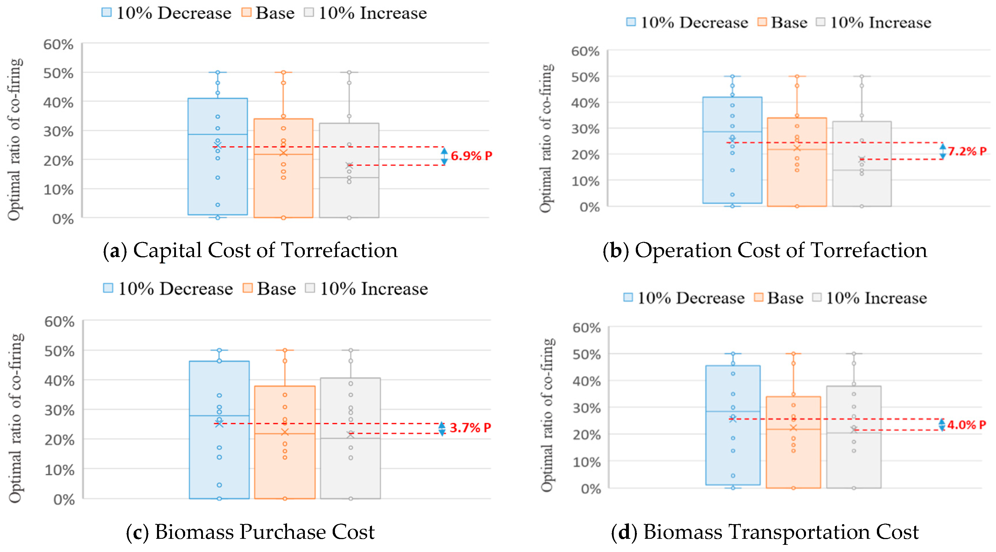
Cost of some of the key parameters, such as feedstock purchasing and torrefaction, are considered fixed in this research. To investigate the impact of cost variations, sensitivity analysis is conducted for four costs parameters; biomass purchasing, biomass transportation (truck/rail), capital costs of torrefaction, and operational costs of torrefaction. In the sensitivity analysis, the optimal level of biomass co-firing for all 26 power plants are re–calculated after each cost factor is independently decreased or increased by 10%. The sensitivity analysis is conducted only for scenario 3 that has advanced logistics system, but no tax credit.

Figure 9 illustrates the changes of optimal level of co-firing based on ±10% cost variations, indicating both the average and the 25%/75% values. The 10% of cost change of an individual parameter has an overall effect of 3.7–7.2% point in the co-firing ratio. This percentage indicates the average change for all 26 coal power plants. The percent change on individual power plants varies. Based on the figure, variation in capital and operation cost for torrefaction in the depots have the greatest effect on the overall level of co-firing ratio. For example, if capital and operational cost of torrefaction changes by ±10%, the average co-firing ratio for all 26 power plants would change on average by 6.9% and 7.2% point, respectively (Figure 9a,b). On the other hand, ±10% change of biomass purchasing cost would lead to comparatively smaller average change of 3.7% point of biomass co-firing (Figure 9c). Biomass transportation costs (both truck and rail) are also less significant than costs related to torrefaction process (Figure 9d).

One interesting aspect of the sensitivity analysis outcomes is to compare them with sensitivity analysis conducted in an earlier study [36]. In the earlier study, the co-firing ratio was kept fixed and changes in advanced logistics system costs were calculated, based on the ±10% cost change of the parameters identified above. Based on those analyses, biomass transportation cost was one of the most sensitive factors for cost variation at the fixed co-firing ratio [36]. However, as indicated in Figure 9, torrefaction cost is more critical for selecting the optimal level of biomass co-firing.

4. Conclusions

This study explores the level of woody biomass co-firing in existing coal power plants considering advanced logistics with torrefaction option. A large MILP with deterministic equivalent of a stochastic problem is developed to determine optimal ratio of woody biomass co-firing at a coal power plant that minimizes logistics costs. This model also includes the constraints relating to the seasonality of biomass and loss of boiler efficiency.

Our model is tested on 26 existing coal power plants in three Great Lakes States. We investigate four different scenarios, separated by the woody biomass logistics system and/or potential tax credit availability. The results reveal that no power plants would use co-firing at the current operational situation, i.e., conventional woody logistics system with no tax credit. The availability of tax credit with conventional logistics system would lead to increase in the use of biomass, but the effect is limited to the low capacity power plants. When advanced logistics system with torrefaction option is provided, the level of biomass co-firing expands to larger capacity power plants. The results also show that high capacity power plants with low delivered costs of coal and poor availability of biomass nearby are not suitable for biomass co-firing, even with advanced logistics system and tax credit.

Sensitivity analysis is conducted to investigate the impact of ±10% cost variations of four different parameters. Based on the analysis, the impact for the co-firing ratio ranges between 3.7–7.2% points, depending on the plant. The sensitivity analysis also reveals that change in capital and operation costs of torrefaction in the depots have highest impact on co-firing ratio.

Although this study uses as much local/regional data as possible, it is recognized that the current model has several shortcomings. It is recognized that several assumptions are used, such as the linear adjustment of capital and operation cost of torrefaction for different capacities. Also, we only concentrated on addressing the complete costs of logistics, so the potential indirect benefits from biomass co-firing to society, such as increase in local job creation, are not within our study boundary. It should also be noted that feedstock logistics cost is only a part of the overall co-firing decision analysis, so this model should be integrated with other technical aspects, such as ash deposition and corrosion rate of utility boilers. Further research is needed to remedy these shortcomings and decrease assumptions needed.

References

- U.S. EIA. Annual Energy Outlook; U.S. EIA: Washington, WA, USA, 2014.
- Basu, P.; Butler, J.; Leon, M.A. Biomass co-firing options on the emission reduction and electricity generation costs in coal-fired power plants. Renew. Energy 2011, 36, 282–288. [Google Scholar] [CrossRef]
- Tillman, D.A. Biomass cofiring: The technology, the experience, the combustion consequences. Biomass Bioenergy 2000, 19, 365–384. [Google Scholar] [CrossRef]
- Roni, M.S.; Eksioglu, S.D.; Searcy, E.; Jha, K. A supply chain network design model for biomass co-firing in coal-fired power plants. Transp. Res. Part E Logist. Transp. Rev. 2014, 61, 115–134. [Google Scholar] [CrossRef]
- Sondreal, E.A.; Benson, S.A.; Hurley, J.P.; Mann, M.D.; Pavlish, J.H.; Swanson, M.L.; Weber, G.F.; Zygarlicke, C.J. Review of advances in combustion technology and biomass cofiring. Fuel Process. Technol. 2001, 71, 7–38. [Google Scholar] [CrossRef]
- National Renewable Energy Laboratory (NREL). Biomass Cofiring in Coal-Fired Boilers. In Federal Energy Management Program; NREL: Golden, CO, USA, 2004. [Google Scholar]
- Fernando, R. Cofiring High Ratios of Biomass with Coal; IEA Clean Coal Centre: London, UK, 2012; Volume 300, p. 194. [Google Scholar]
- Mendell, C.B.; Haber, J.A.; Sydor, T. Evaluating the potential for shared log truck resources in middle Georgia. South. J. Appl. For. 2006, 30, 86–91. [Google Scholar]
- Carlsson, D.; Rönnqvist, M. Backhauling in forest transportation: Models, methods, and practical usage. Can. J. For. Res. 2007, 37, 2612–2623. [Google Scholar] [CrossRef]
- Rentizelas, A.A.; Li, J. Techno-economic and carbon emissions analysis of biomass torrefaction downstream in international bioenergy supply chains for co-firing. Energy 2016, 114, 129–142. [Google Scholar] [CrossRef]
- Van der Stelt, M.J.C.; Gerhauser, H.; Kiel, J.H.A.; Ptasinski, K.J. Biomass upgrading by torrefaction for the production of biofuels: A review. Biomass Bioenergy 2011, 35, 3748–3762. [Google Scholar] [CrossRef]
- Dutta, A.; Leon, M.A. Pros and Cons of Torrefaction of Woody Biomass; University of Guelph, Joint eco ETI & CEF projects workshop Turfgrass Institute: Guelph, ON, Canada, 2011. [Google Scholar]
- Ghenai, C.; Janajreh, I. CFD analysis of the effects of co-firing biomass with coal. Energy Convers. Manag. 2010, 51, 1694–1701. [Google Scholar] [CrossRef]
- Levendis, Y.A.; Joshi, K.; Khatami, R.; Sarofim, A.F. Combustion behavior in air of single particles from three different coal ranks and from sugarcane bagasse. Combust. Flame 2011, 158, 452–465. [Google Scholar] [CrossRef]
- Gubba, S.; Ingham, D.B.; Larsen, K.J.; Ma, L.; Pourkashanian, M.; Tan, H.Z.; Williams, A.; Zhou, H. Numerical modelling of the co-firing of pulverised coal and straw in a 300 MWe tangentially fired boiler. Fuel Process. Technol. 2012, 104, 181–188. [Google Scholar] [CrossRef]
- Álvarez, L.; Yin, C.; Riaza, J.; Pevida, C.; Pis, J.J.; Rubiera, F. Biomass co-firing under oxy-fuel conditions: A computational fluid dynamics modelling study and experimental validation. Fuel Process. Technol. 2014, 120, 22–33. [Google Scholar] [CrossRef]
- Berggren, M.; Ljunggren, E.; Johnsson, F. Biomass co-firing potentials for electricity generation in Poland—Matching supply and co-firing opportunities. Biomass Bioenergy 2008, 32, 865–879. [Google Scholar] [CrossRef]
- Ekşioğlu, S.D.; Karimi, H.; Ekşioğlu, B. Optimization models to integrate production and transportation planning for biomass co-firing in coal-fired power plants. IIE Trans. 2016, 48, 901–920. [Google Scholar] [CrossRef]
- Bergman, P.C.A.; Prins, M.J.; Boersma, A.R.; Ptasinski, K.J.; Kiel, J.H.A.; Janssen, F.J.J.G. Torrefaction for Entrained-Flow Gasification of Biomass; ECN: Petten, The Netherlands, 2005. [Google Scholar]
- Nikolopoulos, N.; Isemin, R.; Atsonios, K.; Kourkoumpas, D.; Kuzmin, S.; Mikhalev, A.; Nikolopoulos, A.; Agraniotis, M.; Grammelis, P.; Kakaras, E. Modeling of wheat straw torrefaction as a preliminary tool for process design. Waste Biomass Valoriz. 2013, 4, 409–420. [Google Scholar] [CrossRef]
- Arteaga-Pérez, L.E.; Segura, C.; Espinoza, D.; Radovic, L.R.; Jiménez, R. Torrefaction of Pinus radiata and Eucalyptus globulus: A combined experimental and modeling approach to process synthesis. Energy Sustain. Dev. 2015, 29, 13–23. [Google Scholar] [CrossRef]
- Bach, Q.-V.; Skreiberg, Ø.; Lee, C.-J. Process modeling and optimization for torrefaction of forest residues. Energy 2017, 138, 348–354. [Google Scholar] [CrossRef]
- Svanberg, M.; Olofsson, I.; Flodén, J.; Nordin, A. Analysing biomass torrefaction supply chain costs. Bioresour. Technol. 2013, 142, 287–296. [Google Scholar] [CrossRef] [PubMed]
- Batidzirai, B.; van der Hilst, F.; Meerman, H.; Junginger, M.H. Optimization potential of biomass supply chains with torrefaction technology. Biofuels Bioprod. Biorefin. 2014, 8, 253–282. [Google Scholar] [CrossRef]
- Boardman, R.D.; Cafferty, K.G.; Nichol, C.; Searcy, E.M.; Westover, T.; Wood, R.; Bearden, M.D.; Cabe, J.E.; Drennan, C.; Jones, S.B.; et al. Logistics, Costs, and GHG Impacts of Utility Scale Cofiring with 20% Biomass; Idaho National Laboratory (INL): Idaho Falls, ID, USA; Pacific Northwest National Laboratory (PNNL): Richland, WA, USA, 2014.
- Office of Energy Efficiency & Renewable Energy. 2016 Billion-Ton Report: Advancing Domestic Resources for a Thriving Bioeconomy, Volume 1: Economic Availability of Feedstocks; Langholtz, M.H., Stokes, B.J., Eaton, L.M., Eds.; Oak Ridge National Laboratory: Oak Ridge, TN, USA, 2016; p. 448.
- Beck, R. Review of Biomass Fuels and Technologies; Yakima County Public Works Solid Waste Division: Yakima, WA, USA, 2003. [Google Scholar]
- Durkay, J. State Renewable Portfolio Standards and Goals. 2017. Available online: http://www.ncsl.org/research/energy/renewable-portfolio-standards.aspx (accessed on 20 December 2017).
- Bracmort, K. Biomass: Comparison of Definitions in Legislation, Congressional Research Service Report 7-5700, R40529; University of North Texas: Denton, TX, USA, 2015. [Google Scholar]
- Pronobis, M.; Wojnar, W. The impact of biomass co-combustion on the erosion of boiler convection surfaces. Energy Convers. Manag. 2013, 74, 462–470. [Google Scholar]
- Miedema, J.H.; Benders, R.M.J.; Moll, H.C.; Pierie, F. Renew, reduce or become more efficient? The climate contribution of biomass co-combustion in a coal-fired power plant. Appl. Energy 2017, 187, 873–885. [Google Scholar]
- IBM. Branch & Cut or Dynamic Search? IBM Knowledge Center 2017. Available online: https://www.ibm.com/support/knowledgecenter/pl/SSSA5P_12.7.1/ilog.odms.cplex.help/CPLEX/UsrMan/topics/discr_optim/mip/performance/13_br_cut_dyn_srch.html (accessed on 15 December 2017).
- Danna, E.; Rothberg, E.; le Pape, C. Exploring relaxation induced neighborhoods to improve MIP solutions. Math. Program. 2005, 102, 71–90. [Google Scholar] [CrossRef]
- IBM. CPLEX User’s Manual, Version 12 Release 7; IBM ILOG CPLEX Optimization; IBM Corp.: New York, NY, USA, 2016. [Google Scholar]
- Lima, R. IBM ILOG CPLEX-What is inside of the box? In EWO Seminar; Carnegie Mellon University: Pittsburgh, PA, USA, 2010. [Google Scholar]
- Ko, S.; Lautala, P. Advanced Woody Biomass Logistics for Cofiring in Existing Coal Power Plant: A Case Study of the Great Lakes States. Transp. Res. Record 2018, in press. [Google Scholar]
- Bureau of Transportation Statistics. Transportation Networks, National Transportation Atlas Database 2015; Bureau of Transportation Statistics: Washington, WA, USA, 2016.
- U.S. EIA. Form 906/920/923: Utility, Non-Utility, and Combined Heat and Power Plant Database; Monthly Time Series; U.S. Energy Information Administration: Washington, WA, USA, 2017.
- U.S. EIA. Form EIA 923 Power Plant Operations Report Instructions; U.S. Energy Information Administration: Washington, WA, USA, 2015.
- The United States Department of Agriculture (USDA). Timber Product Output (TPO) Reports; USDA Forest Service, Southern Research Station: Knoxville, TN, USA, 2012.
- Spelter, H.; McKeever, D.; Toth, D. Profile 2009: Softwood Sawmills in the United States and Canada; U.S. Department of Agriculture Forest Service, Forest Products Laboratory: Madison, WI, USA, 2009; p. 55.
- CN. Canadian National Railway: Prices, Tariffs & Transit Times. 2016. Available online: https://www.cn.ca/en/customer-centre/prices-tariffs-transit-times (accessed on 25 June 2016).
- NS. Norfolk Southern Railway: Public Price Publications. 2016. Available online: http://www.nscorp.com/mktgpublic/publicprices/ (accessed on 25 June 2016).
- U.S. EPA. Biomass Combined Heat and Power Catalog of Technologies; U.S. EPA: Washington, WA, USA, 2007.
- Zhang, L.F.; Johnson, D.M.; Wang, J.J. Integrating multimodal transport into forest-delivered biofuel supply chain design. Renew. Energy 2016, 93, 58–67. [Google Scholar] [CrossRef]
Figure 1.
Processes in advanced woody biomass logistics.
Figure 2.
Combined feedstock supply chain for co-firing power plant.
Figure 3.
Flow chart of MILP optimizer in CPLEX (Adapted from [35]). MILP, mixed integer linear program.
Figure 4.
Feedstock locations, potential terminals, and target coal power plants in Michigan (MI), Wisconsin (WI), and Minnesota (MN).
Figure 5.
Monthly Variations of feedstock supply in study area.
Figure 6.
Biomass co-firing ratio and cost savings by changing logistics system. (a) Results of Biomass Co-firing Ratio; (b) Results of Cost Savings by Advanced Logistics System. PTC, production tax credit.
Figure 7.
Experimental results on the biomass feedstock type and mode of transportation. (a) Scenario 2, Conventional Logistics + PTC (Total Biomass kg: 1.2 Billion); (b) Scenario 3, Advanced Logistics + No PTC (Total Biomass kg: 3.4 Billion); (c) Scenario 4, Advanced Logistics + PTC (Total Biomass kg: 9.6 Billion).